


1. Introduction
In many service systems, capacity may fluctuate over time. For instance, in wireless communication channels this might happen due to mobility of users or fading and interference of signals, and in wired links the capacity allocated to a given flow might evolve depending on cross-traffic. Moreover, it is often the case that the scheduler does not have accurate and instantaneous access to the state of every communication channel.
We study the simple, yet interesting and practically relevant, case when the channel capacity can either be ON or OFF. When the channel is ON, data can be transmitted through the channel with a nonzero probability, but not when it is OFF. Even though the scheduler does not have access to the state of every channel, it does observe successful transmissions. For example, on the internet, with the Transmission Control Protocol (TCP) protocol, the successful transmission of a data packet is acknowledged back to the transmitter. For this model, the scheduler can attempt to keep track of the state by conditioning on the past actions and observations. In the Partially Observable Markov Decision Process (POMDP) literature, this conditional probability distribution over the states of the hidden process is usually called a belief state.
We consider a system with  $K$ independent channels. Time is discrete, and we let
 $p_k$ (
 $q_k$),
 $k=1, \ldots, K$, denote the probability that channel
 $k$ transitions from ON to OFF (OFF to ON), respectively. This Markov chain model is often referred to as the Gilbert–Elliot model [7]. In this setting, the evolution of the channel’s capacity is positively (negatively) autocorrelated if the channel is more (less) likely to be ON if its last state was ON than if its last state was OFF, that is, if
 $1-p_k \gt q_k$ (
 $1-p_k \lt q_k$). Thus, the sign of the autocorrelation is determined by the sign of
 $1-q_k-p_k$. Negative autocorrelation can naturally arise in real-world systems that operate in discrete time (e.g., slotted communication protocols or periodic scheduling systems) in which states alternate frequently. If channel
 $k$ is ON and is selected, a successful transmission occurs (i.e., it is successfully received) with probability
 $\mu_k$. (We assume an infinite number of waiting messages for all channels.) Channels that are OFF do not transmit packets.
We consider non-preemptive service, that is, decision epochs occur immediately after a successful channel transmission, at which time only one channel can be selected and remains activated until the next decision epoch, that is, when another successful transmission occurs. An equivalent interpretation of our problem is non-preemptive scheduling of messages consisting of a geometrically distributed number of packets on channels that always transmit successfully when they are ON. Here,  $\mu$ is the parameter of the geometric distribution instead of the probability of successful transmission. Since the controller does not know the message length in advance, the memoryless property of the geometric distribution implies that, at each ON state, there is a probability
 $\mu$ that the transmitted packet is the last one in the message. The nonpreemption constraint may be desirable in practice, as it reduces the overhead associated with channel switching or transmission restarts.
We denote by  $\pi_k(t)$ the belief state, that is, the probability that channel
 $k$ is ON at time
 $t$ based on the history of successful transmissions, and we let
 $\mathbb{E}[S_k(\pi_k)]$ denote the expected service time—the time between the first selection of the channel and a successful transmission—for channel
 $k$ conditioned on the belief state at the beginning of service being
 $\pi_k$. In particular,
 $\mathbb{E}[S_k(1-p_k)]$ denotes the expected service time for channel
 $k$ assuming channel-
 $k$ is reactivated immediately after a successful transmission in channel
 $k$ (the belief state is
 $1-p_k$ after a successful transmission).
Our main objective is to characterize the scheduling policy that maximizes the long-run rate of successful transmissions, that is, the throughput.
We show that when all channels are positively autocorrelated, the optimal policy is static. We call it the Serve the Best Channel (SBC) policy; it always serves the channel that minimizes  $\mathbb{E}[S_k(1-p_k)]$. The negatively autocorrelated case—when all channels are negatively autocorrelated—is significantly more difficult. We show that for two symmetricFootnote 1 negatively autocorrelated channels, the myopic Largest Belief State (LBS) policy, that at any decision time serves the channel
 $k^* =\arg\max_k (\pi_k(t))$, is optimal. For asymmetric negative autocorrelation, we show, through an example, that LBS is not optimal. Table 1 provides a summary of the optimality results presented in this paper, where the assumption on the autocorrelation applies to all channels.
We then investigate the impact of our constraints on the performance of our model, namely, the lack of information regarding the channel state and of requiring non-preemptive service. In particular, we define the “Preemption Gain,” that is, the relative improvement in the throughput of the optimal preemptive policy with respect to the optimal non-preemptive one, and, similarly, the “Observability Gain.” Combining known results from the literature with new ones, we characterize these gains in various cases of interest. Our numerical computations demonstrate that these gains can be substantial. In such cases, an interesting question arises. Is it worthwhile to incur additional costs to preempt jobs, or to probe channel states, given the resulting performance gain? We believe this opens up a promising area for further investigation. See Table 2 for a concise summary of the results obtained for these gains, where again the assumption on the autocorrelation applies to all channels, and i.i.d. (independent and identically distributed) is equivalent to 0 autocorrelation for our model.
Below we give a brief overview of related work. In Sections 3 and 4, we introduce our mathematical model and provide preliminary results. Section 5 contains our main results on the optimal scheduling policy. Finally, in Sections 6 and 7, we explore the “Preemption Gain” and the “Observability Gain,” respectively.
A three-page extended abstract of this work was presented at the MAMA 2025 workshop [Reference Hira, Ayesta, Righter and Verloop8].
Optimality results.

Table 1 Long description
Two columns compare assumptions about autocorrelation with the corresponding optimal policy. Under the assumptions row labeled, Positive Autocorrelation with the condition stated as one minus p minus q being greater than zero, the assumptions cell says K arbitrary and Asymmetric, and the optimal policy cell gives an argmin over k of an expected value involving S sub k and one minus p sub k, marked Prop 2. Under the row labeled, Negative Autocorrelation with the condition stated as one minus p minus q being less than or equal to zero, the assumptions cell says K equals 2 and Symmetric, and the optimal policy cell gives an argmax over k of pi sub k as a function of t, marked Prop 3.
Gain results.

Table 2 Long description
Columns are Assumptions, Autocorrelation, and Result, with two row groups labeled Preemption Gain and Observability Gain. For Preemption Gain, the assumption is two symmetric classes. Under positive autocorrelation, the result is bounds, Prop 7. Under negative autocorrelation, the result is bounds, Prop 8. For Observability Gain, under an arbitrary number of symmetric classes with positive autocorrelation, the result is closed form, Cor 2. Under two symmetric classes with negative autocorrelation, the result is closed form, Prop 3 part 1. Under two asymmetric classes with independent and identically distributed autocorrelation, the result is closed form, Prop 3 part 2.
2. Related work
There is an extensive literature, mainly in the context of wireless and satellite communications, dealing with scheduling in systems with time-varying capacities, see [Reference Borst5, Reference Tassiulas and Ephremides15] for examples. Another related body of literature is that of queueing systems in a random environment, see [Reference Baccelli and Makowski4]. Here, the parameters of the (modulated) queuing model (including arrival rates and service rates) change over time as a function of an exogenous stochastic process. The scheduler has full information on the state of the system, and the main focus has been on analyzing steady-state properties, such as queue-length distributions. Our model can be seen as a particular instance of a modulated queue or time-varying system, where the service rate of channel  $k$ fluctuates between 0 and
 $\mu_k$, but with partial information.
A nice introduction to the role of information in scheduling, mostly in the context of stability, is provided in [Reference Asanjarani and Nazarathy3]. This paper shows how the problem can be cast as a POMDP, and observes that in full generality there is very little that can be said.
A number of papers have considered systems in which the probability of success when channel  $k$ is ON,
 $\mu_k$, is always 1, for all
 $k$. In this case, the state of the selected channel becomes known whenever it is selected. For example, [Reference Koole, Liu and Righter9] shows that LBS is optimal among preemptive policies for
 $K$ independent symmetric channels, under certain assumptions. These assumptions were relaxed by Ahmad and Liu [Reference Ahmad, Liu, Javidi, Zhao and Krishnamachari2] and Zhao et al. [Reference Zhao, Krishnamachari and Liu19], who proved the optimality of LBS when the channels are positively autocorrelated for
 $K \leq 3$, and showed that LBS is not optimal for negatively autocorrelated channels when
 $K=4$. Ross [Reference Ross14] provides an alternative proof when
 $K=2$ for both positively and negatively autocorrelated channels. See also [Reference Ahmad and Liu1], which considers the possibility of sensing multiple channels, and [Reference Liu and Zhao11] and [Reference Wang and Chen16], which consider nonsymmetric channels.
The assumption that  $\mu_k \equiv 1$ was relaxed in [Reference Liu, Zhao and Krishnamachari12], where states are observed only upon receipt of a randomly produced reward, and conditions were given for the optimality of LBS for two symmetric channels assuming preemption. This was generalized to
 $K \ge 2$ symmetric channels in [Reference Wang, Chen, Liu and Agha18], and to nonsymmetric channels in [Reference Wang, Chen and Liu17]. In a recent paper, Liu et al. [Reference Liu, Weber and Zhang10] consider a similar model to that of [Reference Liu, Zhao and Krishnamachari12] and calculate (approximately) the Whittle index. We further refer to [Reference Asanjarani and Nazarathy3], where instead of ON and OFF states, channels can be “good” or “bad,” so a successful transmission might occur, but with a lower probability, even in the bad state, and where the impact of partially observable channels on stability is studied.
All of the work cited above concerns preemptive scheduling. To the best of our knowledge, our work is the first dealing with the non-preemptive setting. As noted in the introduction, in Sections 6 and 7 we will compare our results with those obtained in the preemptive case as well as in the case with perfect observation.
Regarding observability, our findings complement the insights of [Reference Duran and Verloop6], which showed that in a multi-armed restless bandit problem with a random observable environment, the Average Whittle policy defined therein (which does not require channel state observation) achieves asymptotic optimality as the environments’ dynamics become very fast. In other words, as we have a timescale separation, the Observability Gain converges to zero. In contrast, our results will show that the Observability Gain can be significant in non-asymptotic regimes, highlighting the critical value of channel state information for the performance of scheduling policies.
3. Model description
We consider a discrete-time scheduling problem with an infinite number of waiting jobs and  $ K $ channels, only one of which can be selected (or served, or activated) in each time slot. Channel
 $k$ has an independent associated Markov chain process
 ${X_k}$ describing its environment with two states: “ON” and “OFF,” and the corresponding transition matrix is
 $P_k = \begin{bmatrix} 1-p_k & p_k \\ q_k & 1- q_k \end{bmatrix}$. It is easy to show that channel
 $k$ has positive (negative) autocorrelation when
 $1-p_k-q_k\geq 0$ (
 $1-p_k-q_k\leq 0$), and that channel states are i.i.d. if
 $1-p_k-q_k=0$. Indeed, letting
 $\stackrel{\sim}{X}_{k}(t)=I\{X_{k}(t)=ON\}$, we have
 \begin{align*}
\operatorname{Cov}(\stackrel{\sim}{X}_k(t),\stackrel{\sim}{X}_k(t+1))&=\mathbb{E}[\stackrel{\sim}{X}_k(t)\stackrel{\sim}{X}_k(t+1)]-\mathbb{E}[\stackrel{\sim}{X}_k(t)]\mathbb{E}[\stackrel{\sim}{X}_k(t+1)] \\
&=\mathbb{P}[\stackrel{\sim}{X}_k(t)=\ \stackrel{\sim}{X}_k(t+1)=1]-\mathbb{P}[\stackrel{\sim}{X}_k(t+1)=1]\mathbb{P}[\stackrel{\sim}{X}_k(t)=1] \\
&=\Big(\mathbb{P}[\stackrel{\sim}{X}_k(t+1)=1|\stackrel{\sim}{X}_k(t)=1]-\mathbb{P}[\stackrel{\sim}{X}_k(t+1)=1]\Big)\mathbb{P}[\stackrel{\sim}{X}_k(t)=1] \\
&= \Delta \mathbb{P}[\stackrel{\sim}{X}_k(t)=1],
\end{align*}
with
 \begin{align*}
\Delta &=\mathbb{P}[\stackrel{\sim}{X}_k(t+1)=1|\stackrel{\sim}{X}_k(t)=1]-\mathbb{E}\big[\mathbb{P}[\stackrel{\sim}{X}_k(t+1)=1|\stackrel{\sim}{X}_k(t)]\big] \\
&=(1-p)-\Big((1-p)\mathbb{P}[\stackrel{\sim}{X}_k(t)=1]+q\big(1-\mathbb{P}[\stackrel{\sim}{X}_k(t)=1]\big)\Big) \\
&=(1-p-q)\Big(1-\mathbb{P}[\stackrel{\sim}{X}_k(t)=1]\Big)
\end{align*}
so the sign of the covariance depends only on the sign of  $1-p-q$. Also recall that Bernoulli random variables are independent if they have zero correlation.
The activation process is non-preemptive, meaning that once a channel is activated, the job at the head of the queue must be served to completion before another channel can be activated. As a result, decision times,  $t_n$, correspond to the time slots immediately after job completions.
An action at decision time  $t_n$ is
 $u(t_n) \in \{0,...,k\}$, where
 $u(t_n)=k$ corresponds to activating channel
 $k$ and
 $u(t_n)=0$ corresponds to idling. We refer to the function
 $u$ as a policy. We also define, for times
 $t$ that are not decision times,
 $u(t) = k$ if
 $k$ is the currently active channel, that is,
 $u(t) = u(t_n)$ for
 $t_n \in [t_n, t_{n+1}) $. An active channel
 $k$ that is “ON” (i.e.,
 $u(t)=k$ and
 $X_k(t)=$ ON) results in a service completion (i.e., yields a reward of
 $1$) with probability
 $\mu_k$, while any other scenario results in no reward.
The controller cannot observe the states of the channels  $X_k$, but it can observe service completions, and it knows the parameters
 $p_k$,
 $q_k$,
 $\mu_k$ of the model, as well as the currently active channel, so we have a POMDP formulation. The controller’s belief state at time
 $t$ is denoted by
 $ \pi (t)= (\pi_1 (t), \ldots, \pi_K (t)) \in [0,1]^K $, where each
 $ \pi_k (t) $ is the controller’s belief probability of channel
 $k$ being in the “ON” state. The belief-state update mechanism will be made precise in Section 4.1. The reward at time
 $t$ when channel
 $k$ is active (
 $u(t)=k$) is
 \begin{align*}
& R_t\big(k) := \begin{cases}
I\{X_k(t)=ON\} \text{ with probability } \mu_k,\\
\text{ 0 otherwise.}
\end{cases}
\end{align*}
The decision times  $t_0, t_1,\ldots,$ are therefore random variables depending on the policy
 $u$ employed:
 \begin{align*}
\begin{cases}
t_0 = 0, \\
t_{n+1} = \inf \{t \gt t_n \ | \ R_{t-1}( u(t-1))=1 \}.
\end{cases}
\end{align*}
In Lemma 4 we will see that idling is never optimal for our model, so each successful transmission time will correspond to an activation decision. Define
 \begin{equation*}U:= \left\{\ u(t) \ | \ \forall t, \ u(t)\in\{0,1...,K\}, \ R_t( u(t) )=0 \Rightarrow u(t+1) = u(t)
\right\},\end{equation*}
as the space of non-preemptive policies  $u(\cdot)$. We denote by
 $g^u$ the expected average reward (the transmission rate or throughput) of a policy
 $u \in U$, that is,
 \begin{align*}
g^u := \lim_{T \to \infty } \mathbb{E}\left[ \frac{1}{T} \sum_{t=0}^{T-1} R_t( u(t) ) \right]
= \lim_{T \to \infty } \left[ \frac{1}{T} \sum_{t=0}^{T-1} \pi_{u(t)}\mu_{u(t)} \right],
\end{align*}
and by  $g^*$ the optimal expected average reward,
 \begin{align*}
g^* := \max_{u \in U}g^u.
\end{align*}
Our objective is to find a policy that is in the set of average optimal policies. This model is illustrated in Figure 1.
 \begin{equation*} U^* := \{u \in U \ | \ g^{u}=g^* \}.\end{equation*}
Illustration of our model.

4. Preliminary results
4.1. Probability updating
The belief state is updated as follows:
 \begin{equation*}
\pi_k(t+1) =
\begin{cases}
1-p_k & \text{ if } u(t) = k , R_t(k ) = 1 \\
\overline{T}_k(\pi_k(t)) & \text{ if } u(t) = k , R_t(k ) = 0 \\
T_k(\pi_k(t)) & \text{ if } u_(t) \ne k,
\end{cases}
\end{equation*}
with  $T_k$ and
 $\bar T_k$ defined below in (1) and (2). To explain the first case, note that if a channel is active at time
 $t$ and there is a service completion, then we know it was in state ON at time
 $t$, and the probability that it is in state ON at time
 $t+1$ is therefore indeed
 $\mathbb{P}[X_k(t+1)=ON | X_k(t)= ON] = 1-p_k$.
For the second case,  $ T_k(\pi_k(t)) $ denotes the updated probability of channel
 $k$ being “ON,” given that it was not activated, that is,
 \begin{align}
T_k(\pi_k) &:= \mathbb{P}\left[X_k(t+1) = \text{ON} | \pi_k(t) = \pi_k ; u_k(t) = 0\right]
\\ \nonumber
&= (1-p_k) \pi_k + q_k (1-\pi_k) = \pi_k(1-p_k-q_k) + q_k.\end{align}
Similarly,  $ \overline{T}_k $ denotes the updated probability of the channel being “ON” when the channel was activated but no service completion (departure) was observed, that is,
 \begin{align}
\overline{T}_k(\pi_k) &:= \mathbb{P}\left[X_k(t+1) = \text{ON} | \pi_k(t) = \pi_k ; u_k(t) = 1 ; R_t(\pi_k(t) , u_k(t) ) = 0\right] \\ \nonumber &= \frac{(1-\mu_k)\pi_k (1-p_k) + (1-\pi_k)q_k}{1-\pi_k \mu_k}
= \frac{\pi_k(1-p_k-q_k-\mu_k(1-p_k))+q_k}{1-\mu_k \pi_k}.\end{align}
We note that the updating functions  $T_k(\cdot)$ and
 $\overline T_k(\cdot)$ are both increasing (decreasing) as a function of
 $\pi_k$ when
 $1-p_k-q_k \gt 0$ (
 $1-p_k-q_k \lt 0$ respectively).
Due to the non-preemptive nature of a policy, the term  $T_k^i(1-p_k)$ is of particular interest to us as it represents the conditional probability—or in POMDP terminology, the controller’s belief—of the channel’s state being ON
 $i+1$ steps after a departure from channel
 $k$ while not being served. We have the following result.
Lemma 1. For  $i\in \mathbb{N}$,
 \begin{equation*}T_k^i(1-p_k)=(1-p_k-q_k)^i(1-p_k-\frac{q_k}{p_k+q_k}) + \frac{q_k}{p_k+q_k}.\end{equation*}
Proof. The proof follows by induction. We have  $T^0(1-p_k)=1-p_k$. Now assume the result holds for
 $i-1 \gt 0$. We then have, from Eq. (1),
 \begin{align*}
T_k^{i}(1-p_k) & = T_k^{i-1}(1-p_k)(1-p_k-q_k) + q_k \\ &= (1-p_k-q_k)^{i}(1-p_k-\frac{q_k}{p_k+q_k}) + \frac{q_k}{p_k+q_k}(1-p_k-q_k) +q_k \\ & = (1-p_k-q_k)^{i}(1-p_k-\frac{q_k}{p_k+q_k}) + \frac{q_k}{p_k+q_k}.
\end{align*}
In Figure 2, we plot the value of  $T_k^i(1-p_k)$ as a function of the number of steps since the last departure,
 $i+1$, for both positively and negatively autocorrelated channels. For example, when
 $i=0$, the channel just observed a departure; hence, the belief state is
 $1-p_k$. As we noted in the introduction, positive (negative) autocorrelation occurs when the process tends to stay in the same state with higher (smaller) probability than an i.i.d. process would. Hence, in the case of positive autocorrelation, after one step (so
 $i=0$) the probability of being ON is highest, then decreases to the equilibrium probability. In the negatively autocorrelated case, oscillations appear, dampening as the ON probability converges to its equilibrium,
 $ \frac{q_k}{p_k+q_k}$.
Belief state evolution  $T_k^i(1-p_k)$ for (left) a positively autocorrelated channel (
 $1 - p_k - q_k \gt 0$) and (right) a negatively autocorrelated channel (
 $1 - p_k - q_k \lt 0$).

We note that our later results will depend not only on the correlation,  $1-p_k-q_k$, but also on
 $1-p_k-\frac{q_k}{p_k+q_k}=T^0(1-p_k)-T^{\infty}(1-p_k)$, the difference between the posterior belief states depending on whether the last departure was one time step ago or a long time ago.
4.2. Effective service time
We define the effective service time of an activated channel as a function of the initial belief state,  $\pi_k$, as the (random) time from the start of service until its completion:
 \begin{align*}
S_k(\pi_k) := \inf \{s \geq 1 \ ; \ R_s(\overline{T}_k^{s-1}(\pi_k),1)=1 \}.
\end{align*}
The decision times for a given policy  $u$ are given by
 $t_{n+1}=t_n+S^u_{t_n}$, where
 $S^u_t$ denotes the effective service time under policy
 $u$ when the job starts being served at time
 $t$, so
 $S^u_t \sim S_{u(t)}(\pi_{u(t)}(t))$. We now provide a closed-form expression for the moment-generating function of the effective service time. The proof can be found in Appendix A.
Proposition 1. For  $\rho \in \mathbb{R}$, we have
 \begin{equation*}\mathbb{E} [ \rho^{S_k(\pi_k)} ] = \sum_{n=1}^{\infty} \rho^n \mu_k \overline{T}_k^{n-1}(\pi_k) \prod_{j=0}^{n-2} (1-\mu_k \overline{T}_k^{j}(\pi_k)) = C_k(\rho) + D_k(\rho)\pi_k, \end{equation*}
and
 \begin{equation*}\mathbb{E}[S_k(\pi_k)] = \frac{p_k+q_k+\mu_k(1-p_k-\pi_k)}{\mu_k q_k},\end{equation*}
where
 \begin{equation*}C_k(\rho):= \frac{\mu_k \rho^2 q_k }{1-\rho(2-p_k-q_k-\mu_k(1-p_k)) + \rho^2(1-p_k-q_k)(1-\mu_k)},\end{equation*}
 \begin{equation*}D_k(\rho) := \frac{\mu_k \rho (1-\rho) }{1-\rho(2-p_k-q_k-\mu_k(1-p_k)) + \rho^2(1-p_k-q_k)(1-\mu_k)}.\end{equation*}
Note that  $E[S_k(\pi_k)]$ is decreasing in
 $\pi_k$. Since we consider non-preemptive policies, an important quantity will be the expected effective service time of a channel at a decision time. We thus define
 $\mathbb{E}[S_k(T_k^i(1-p_k))]$ as the expected effective service for channel
 $k$ given the last successful transmission for channel
 $k$ happened
 $i$ time units ago.
 \begin{equation*}\mathbb{E}[S_k(T_k^i(1-p_k))] = A_k + B_k(1-p_k-q_k)^i, \end{equation*}
where  $A_k:=\frac{p_k+q_k+\mu(1-p_k-\frac{q_k}{p_k+q_k})}{\mu q_k}$ and
 $B_k:= -\frac{1-p_k-\frac{q_k}{p_k+q_k}}{q_k}.$
Proof. The result follows from Lemma 1 and Proposition 1.
4.3. Optimal scheduling policies
In this section, we discuss and characterize optimal scheduling policies. We first recall that our objective is to find policies that maximize the average reward, where the reward received is 1 each time a job departs. Let
 \begin{equation*}\overline{S}^u := \lim_{N \to \infty} \frac{1}{N}\sum_{n=0}^N S^u_{t_n}\end{equation*}
be the average effective service time under policy  $u$. In the following lemma, we show that the average reward is inversely proportional to the average service time. For the sake of completeness, we provide a proof in Appendix B.
Lemma 3. For  $u \in U$,
 $g^u = \left(\overline{S}^u\right)^{-1}$. As a consequence, a policy minimizing the expected effective service time is average optimal, that is,
 $\stackrel{\sim}{u}\ \ = \arg \min_{u \in U} \overline{S}^u \Longleftrightarrow \stackrel{\sim}{u}\ \ \in U^*.$
This lemma allows us to find an average-optimal policy by solving the Bellman equation for the effective service time.
Corollary 1. If the index  $k^*(\pi)$ minimizes the right-hand side of the following Bellman equation:
 \begin{align*}
&\phi(\pi)+\overline{S}^* \\ &= \min_{k} \left( \mathbb{E}[S_k(\pi_k)] + \mathbb{E}[\phi(T_1^{S_k(\pi_k)}(\pi_1), ... , T_{k-1}^{S_k(\pi_k)}(\pi_{k-1}),1-p_k,T_{k+1}^{S_k(\pi_k)}(\pi_{k+1}),...,T_{K}^{S_k(\pi_k)}(\pi_K) )]\right),\nonumber
\end{align*}
then, for all decision times  $t$, the policy
 $u^*(t) = \begin{cases}
u_k(t) = 1 \text{ if } k=k^*(\pi(t)) \\
u_k(t) = 0 \text{ otherwise}
\end{cases}$ belongs to
 $U^*$.
Proof. Dynamic programming results (e.g., [Reference Puterman13]) establish that any Bellman-optimal policy (a policy satisfying the right-hand side of the Bellman equation) is also average optimal. Together with Lemma 3, we can conclude the proof.
In the search for optimal policies, we first prove that we can focus on non-idling policies. We will see later that when we relax our non-observability assumption, idling may sometimes be optimal.
Lemma 4. An average-optimal policy will be non-idling, that is,  $u^*(t) \in \{1,...,k\} \forall t$.
Proof. We give a sample-path proof by contradiction. Suppose at some time  $t$ we decide to idle for some time
 $i$. Note that we will have no new information at time
 $t+i$, that is, we can compute the belief states for time
 $t+i$ at time
 $t$. In other words, we can decide at time
 $t$ which channel we will serve, say channel
 $k$, at time
 $t+i$. We can thus compare two policies: Policy
 $u_1$ idles until time
 $t+i$ and then serves channel
 $k$. Policy
 $u_2$ serves channel
 $k$ right away and keeps serving channel
 $k$ until the next decision time greater than
 $t+i$, even if there are successful transmissions before time
 $t+i$. We couple the states of the channels and the (potential) transmissions under the two policies. So from
 $t+i$ onward, policy
 $u_1$ and policy
 $u_2$ will serve the same channel
 $k$. This implies a departure will happen for both policies
 $u_1$ and
 $u_2$ at some given time
 $t+i+s$. The belief state of channel
 $k$ is thus reset to
 $1-p$ for both policies, and no other channels have been served since
 $t+i$, so their belief states will also be the same at
 $t+i+s$. But now, because policy
 $u_2$ started serving channel
 $k$ before policy
 $u_1$, there may have been some successful transmissions before time
 $t+i$ for policy
 $u_2$ (but not for
 $u_1$). Hence, the total reward of policy
 $u_2$ is at least as large as policy
 $u_1$.
This lemma allows us to conclude that upon departure of a job, an optimal policy immediately chooses a new channel to serve. The question is thus which channel to serve given the current belief states  $\pi_k$, for all
 $k$. Results on optimal control policies will be proved in the next section.
5. Optimality results
In this section, we derive average-optimal policies for both positively and negatively autocorrelated channels.
Our results show that the structure of the optimal policy is very different depending on the nature of the autocorrelation. This is not surprising given that the evolution over time of the belief state is radically different in the positive and negative autocorrelation cases, see Figure 2. Additionally, we provide closed-form expressions for the expected average reward associated with the obtained optimal policies.
To obtain the optimal policy, one needs to strike the right balance between short-term and long-term rewards. In the short term, the greedy action would be to serve the channel having the smallest expected effective service time,  $\mathbb{E}(S_k(\pi_k)),$ that is,
 $k^*$ with
 $k^*=\arg\min \mathbb{E}(S_k( \pi_k))$. In the longer term, it might be beneficial to serve some other channel
 $\stackrel{\sim}{k}\neq k^*$. Once such channel
 $\stackrel{\sim}{k}$ has a departure, its belief state is reset to
 $1-p_{\stackrel{\sim} k}$, and its belief state evolution (see Figure 2) can potentially see higher values than those before it was served. We will see such an example in Sections 5.1 and 5.3. A setting where the greedy policy is in fact optimal is given in Section 5.2.
5.1. Positively autocorrelated channels
When, for all  $k$, the channels’ environments are positively autocorrelated, that is
 $1-p_k-q_k\geq 0$, the belief state for a channel to be ON is decreasing in the number of steps since the last departure. Hence, the corresponding expected service time
 $\mathbb{E}[S_k(T^i_k(1-p_k))]$ is increasing in
 $i$. We recall that at a decision time, a job just departed from some channel
 $k$, so its belief state is
 $1-p_{k}$ and its expected service time is
 $\mathbb{E}[S_k(T^0_k(1-p_k))] = \mathbb{E}[S_{k}(1-p_{k})]$. In this section we show that the policy that always serves the channel with the smallest value of
 $\mathbb{E}[S_{k}(1-p_{k})]$, which we call the Serve the Best Channel (SBC) policy, is average optimal. In case of a tie, the SBC policy will choose one of the best channels and use that choice consistently thereafter.
Proposition 2. If  $(1-p_k-q_k) \gt 0$ for all
 $k$, then the SBC policy, which always serves channel
 $k^{\ast }$,
 $u(t) = k^{\ast } \forall t$, where
 \begin{equation*}
k^{\ast }= \operatorname*{argmin}_{k \in \{1,...,K\}}\mathbb{E}[S_k(1-p_k)] = \operatorname*{argmin}_{k \in \{1,...,K\}} \frac{p_{k}+q_{k}}{q_{k}\mu _{k}},
\end{equation*}
is average optimal. In case of a tie, choose one of the minimizing channels arbitrarily, and use this choice consistently thereafter.
The optimal average reward is given by
 \begin{equation*}g^* = g^{SBC} = \mu _{k^{\ast }}\frac{q_{k^{\ast }}}{p_{k^{\ast }}+q_{k^{\ast }}}.\end{equation*}
Proof. Consider a policy  $u$ and its corresponding decision times
 $t_n$,
 $n \gt 0$. Due to the positive autocorrelation, we have that
 $\pi_k(t_n) \leq 1-p_k$ for all
 $k$, from Lemma 1 (see Figure 2). Together with the fact that
 $\mathbb{E}[S_k(\pi_k)]$ is decreasing in
 $\pi_k$, it holds that
 $\mathbb{E}[S_{t_n}^u] = \mathbb{E}[S_{u(t_n)}(\pi_{u(t_n)})] \geq \mathbb{E}[S_{u(t_n)}(1-p_{u(t_n)})] \geq \mathbb{E}[S_{k^*}(1-p_{k^*})]$, where the latter inequality follows by definition of
 $k^*$. We conclude the proof by noting that
 \begin{equation*}\lim_{N \to \infty} \frac{1}{N} \sum_{n=1}^N \mathbb{E}[S_{t_n}^u] \geq \lim_{N \to \infty} \frac{1}{N} \sum_{n=1}^N \mathbb{E}[S_{k^*}(1-p_{k^*})],\end{equation*}
where the RHS is the average service time of SBC, together with Lemma 3.
Remark 1 (SBC is not a greedy policy)
Note that the optimal policy above is not necessarily greedy in the sense of minimizing the expected time to the next service completion for any initial belief states. For example, consider the two channels with parameters as in Figure 3, in which SBC would serve channel 1. Suppose the initial states are such that channel 2 just saw a departure (i.e.,  $i=0$) and channel 1 had a departure
 $i\geq 1$ time slots ago. A greedy policy would now serve channel 2, as this would minimize the mean time to the next service completion. After such a service completion, we will have similar belief states, and again, a greedy policy chooses to serve channel 2. Hence, a greedy policy would never switch from channel 2 to channel 1, and is hence sub-optimal.
Comparison of  $\mathbb{E}[S_{k}(T_k^i(1-p_{k}))]$ for two positively correlated channels with
 $\mu_1=\mu_2=0.9$.

Remark 2 (SBC is a type of “ $\boldsymbol{c \mu}$” policy)

Note that the SBC policy always activates the channel with the maximal value of  $c \mu$, where
 $c = q/(p+q)$ is the long-run proportion of time the channel is in the ON state.
5.2. Two symmetric and negatively autocorrelated channels
In this section, we assume we have two symmetric channels ( $p_k=p,q_k=q$, and
 $\mu_k=\mu$, for
 $k=1,2$) that are negatively autocorrelated,
 $1-p-q \lt 0$. We also assume that both channels have been activated at some point in the past. Hence, at each decision time
 $t$,
 $\pi(t) = (1-p, T^{i}(1-p))$, where we label the channel that just had a service completion as channel 1, without loss of generality, and where
 $i$ is the time since channel 2 last had a service completion.
Due to the symmetry of the channels, combined with the fact that the expected effective service time is decreasing in the belief state, the greedy policy (with respect to  $\mathbb{E}(S_k(\pi_k)) $) simplifies to serving the channel that currently has the LBS. We refer to this policy as the Largest Belief State (LBS) policy. Though the greedy policy might not be optimal in general, below we prove that in the case of two symmetric and negatively autocorrelated channels it is.
Indeed, having symmetry in the channels means that any decision of which channel to serve will reset the corresponding belief state (and future evolution) in the same manner. Hence, there is no trade-off between short term and long term, so an optimal policy is greedy (LBS in this setting). The proof makes use of the Bellman Equation for the service time, see Corollary 1, and can be found in Appendix C.
Proposition 3. If  $K=2$,
 $\mu_k=\mu$,
 $p_k=p$ and
 $q_k=q$, for
 $k=1,2$,
 $1-p-q \lt 0$, then the LBS policy, which for a given belief state
 $\pi$ serves channel
 $k^*$, where
 \begin{equation*}k^*=\arg \max_k(\pi_k),\end{equation*}
is average optimal. Because  $K=2$, LBS simplifies to continuously switching between the two channels.
The challenge in extending the optimality of LBS beyond  $K=2$ lies in the fact that, after following LBS for a single decision epoch, the system transitions to a “worse” state (in terms of belief states) compared to what could result from following a sub-optimal policy (due to the negative autocorrelation). Our proof of Proposition 3 shows that for
 $K=2$, the gain achieved outweighs the losses incurred, but we were unable to generalize this result to arbitrary
 $K \gt 2$. We do, however, conjecture it to be true: numerical simulations up to
 $K=6$ using the value‐iteration algorithm revealed no counterexamples. It is worth noting that in the preemptive case, the optimality of preemptive-LBS for
 $K \gt 2$ has only been established under restrictive technical conditions, see Section 2, highlighting that the difficulty is not specific to our model.
Conjecture 1. For symmetric and negatively correlated channels, LBS is optimal for arbitrary  $K$.
In the next proposition, we characterize the average reward of LBS for two symmetric negatively autocorrelated channels. Its proof can be found in Appendix D.
Proposition 4. For  $K=2$,
 $\mu_k=\mu$,
 $p_k=p$, and
 $q_k=q$, for
 $k=1,2$,
 $1-p-q \lt 0$, the expected average reward under LBS is given by
 \begin{align*}
g^{LBS} = \left( A+B\frac{C+D\frac{q}{p+q}}{1-(1-p-\frac{q}{p+q})D} \right)^{-1},
\end{align*}
with  $C:=C(1-p-q)$ and
 $D:=D(1-p-q)$, and with
 $C(\cdot)$,
 $D(\cdot)$,
 $A$, and
 $B$ as defined in Proposition 1 and Lemma 2.
5.3. Non-optimality of a greedy policy with asymmetric negatively autocorrelated channels
With symmetric and negatively autocorrelated channels, we showed in Proposition 3 that the greedy policy, which reduces to LBS in this case, is average optimal. In this section, we will show, through the example below, that the greedy policy is not necessarily optimal for nonsymmetric negatively autocorrelated channels. Recall that the greedy policy was also not optimal for positively autocorrelated channels, see Remark 1.
Example 1. We consider two channels, where channel 1 is negatively autocorrelated with parameters  $p_1=p$,
 $q_1=q$,
 $1-p-q \lt 0$, and
 $\mu_1=\mu$, and channel 2 is i.i.d. with parameters
 $p_2=p+\epsilon$,
 $q_2=1-p_2$, and
 $\mu_2=\mu$. We fix
 $\epsilon$ such thatFootnote 2
 \begin{equation}
1 - p - \frac{q}{p+q} \lt \epsilon \lt 1 - p - \frac{q}{p+q - \mu\bigl(1 - p - T_1^2(1-p)\bigr)}.
\end{equation}
In Figure 4, we plot, for each channel, the expected service time when service is started at  $i$ time units since the last departure from each channel,
 $\mathbb{E}[S_k(T^i(1-p)]$. Due to the i.i.d. assumption, for channel 2 the latter is constant in
 $i$, and we denote it by
 $\mathbb{E}[S_{iid}^{\epsilon}]$, that is,
 $\mathbb{E}[S_{iid}^{\epsilon}]:=\mathbb{E}[S_2(T^i(1-p)]= \frac{1}{\mu \bigl(1 - p - \epsilon\bigr)}.$
Non-optimality of the greedy policy for an i.i.d. channel and a negatively autocorrelated channel.

The greedy policy serves at each moment in time the channel  $k^*=\arg\min\{\mathbb{E}[S_k(T^i(1-p))]\}$. Since
 \begin{equation*}\mathbb{E}[S_1(T_1^i(1-p))]\leq \mathbb{E}[S_1(1-p)] = \frac{p+q}{\mu q} \leq \frac{1}{\mu \bigl(1 - p - \epsilon\bigr)}=\mathbb{E}[S_{iid}^\epsilon],\end{equation*}
due to  $1 - p - \frac{q}{p+q} \le \epsilon$, this implies that the greedy policy will always serve channel 1, see also Figure 4. The average reward under the greedy policy is therefore
 $\mathbb{E}[S_1(1-p)].$
Now consider the policy that always alternates between channels. A service in channel 2 takes  $S_{iid}^{\epsilon}$ units of time. Hence, the expected service time of channel 1 under this policy equals
 $\mathbb{E}[S_1(T_1^{S_{iid}^{\epsilon}}(1-p))]$, since channel 1 is activated
 $S_{iid}^{\epsilon}$ time units since the last departure from channel 1. By a renewal argument, the average service time under the alternating policy is therefore
 $\frac{1}{2}\bigl(\mathbb{E}[S_{iid}^{\epsilon}] + \mathbb{E}[S_1(T_1^{S_{iid}^{\epsilon}}(1-p))]\bigr).$ The latter can be upper bounded as follows:
 \begin{align*}
\frac{1}{2} \left( \mathbb{E}[S_{iid}^{\epsilon}] + \mathbb{E}[S_1(T_1^{S_{iid}^{\epsilon}}(1-p))] \right)
&\le \frac{1}{2}\left(
\frac{1}{\mu \bigl(1 - p - \epsilon\bigr)} + \mathbb{E}[S_1\bigl(T_1^2(1-p)\bigr)]\right) \\
&=
\frac{1}{2}\left(\frac{1}{\mu \bigl(1 - p - \epsilon\bigr)}
+ \frac{p+q}{\mu q}
+ \frac{1}{q}\bigl(1 - p - T_1^2(1-p)\bigr) \right)\\
& \lt \frac{p+q}{\mu q}
= \,\mathbb{E}[S_1(1-p)],
\end{align*}
where the last inequality follows from (1). Recall that  $1/\mathbb{E}[S_1(1-p)]$ is the average reward under the greedy policy, so the greedy policy is not optimal in this example.
We conclude this section by noting that in general the optimal policy will be difficult to characterize. Already with two asymmetric negatively autocorrelated channels, an optimal policy would need to strike the right balance between short-term and long-term rewards, that is, find the thresholds on the number of steps since the last departure to determine when to switch between channels.
6. Preemptive vs non-preemptive in the symmetric case
In this section, we compare the performance of the optimal preemptive and non-preemptive policies when the state is non-observable, through the Preemption Gain, that is, the relative improvement in the throughput of the optimal preemptive policy with respect to the optimal non-preemptive one. We denote the average reward under the optimal policy in the preemptive model by  $g^{*,preempt}$, and recall that under the optimal policy in the non-preemptive model this is denoted by
 $g^{*}$. We define by
 \begin{equation*}Gain^{preempt} := \frac{g^{*,preempt} - g^{*}}{g^{*}}\end{equation*}
the “Preemption Gain,” which measures how much the average reward increases when preemption is allowed, and thus can be seen as a “Price for Nonpreemption.”
For preemptive models, there exist conditions under which the preemptive-LBS policy (at any moment in time, serve the channel with the LBS) is optimal, see Section 2. In the case of two symmetric channels, Liu et al. [Reference Liu, Zhao and Krishnamachari12] derive bounds for the average reward under preemptive-LBS, which we will use to obtain bounds on  $Gain^{preempt}$. In this section, we will therefore focus on
 $K=2$ and symmetric channels and drop the subscript
 $k$ for notational convenience.
6.1. Results from [Reference Liu, Zhao and Krishnamachari12]
Liu et al. [Reference Liu, Zhao and Krishnamachari12] showed that in the preemptive setting, preemptive-LBS policy is optimal when Condition 1 below is satisfied.
Condition 1.
The parameters satisfy  $\mu \gt 1 -\frac{\min\left(q,1-p\right)\left(1-\max\left(q,1-p\right)\right)}{\max\left(q,1-p\right)\left(1-\min\left(q,1-p\right)\right)}.$ When
 $1-p-q \gt 0$, this simplifies to
 $\mu \gt \frac{1-p-q}{(1-p)(1-q)},$ and when
 $1-p-q \lt 0$, this simplifies to
 $\mu \gt -\frac{1-p-q}{pq}$.
Below we present the bounds obtained in [Reference Liu, Zhao and Krishnamachari12] for the optimal average reward in the preemptive setting.
Proposition 5. [Positive autocorrelation [Reference Liu, Zhao and Krishnamachari12]]
For two symmetric queues, assuming  $1-p-q \gt 0$ and Condition 1, we have the following bounds on the preemptive optimal average reward:
 \begin{align*}
\frac{f\left(c_{1}\right)\mu}{1-\left(1-p-f\left(c_{1}\right)\right)\mu} \leq g^{*,preempt} \leq \frac{\frac{q}{p+q}\mu}{1-(1-p-\frac{q}{p+q})\mu},
\end{align*}
where
 \begin{align*}
f\left(x\right):=\frac{\left(\frac{q}{p+q}-x\right)}{1-x\cdot \mu\cdot\left(1-\frac{\left(1-p-q\right)\left(1-\left(1-p\right)\mu\right)}{1-\left(1-p-q\right)\left(1-p\right)\mu}\right)},
\end{align*}
 $c_1 := \left(\frac{q}{p+q}-c_{2}\right)\left(1-p-q\right)$ and
 $c_{2}:=\frac{q\left(1-q+\left(1-\mu\right)\left(1-p\right)\right)}{1-\mu q}$.
Proposition 6. (Negative autocorrelation [Reference Liu, Zhao and Krishnamachari12])
For two symmetric queues, assuming  $1-p-q \lt 0$ and Condition 1, we have the following bounds on the preemptive optimal average reward:
 \begin{align*}
\frac{1}{ \left( \frac{(2-y_1)\mu q}{(1-y_1)^2} - x_1 \right) h(x_1,y_1,\mu q,a_1,0)+1} \leq g^{*,preempt} \leq \frac{1}{ \left( \frac{(1+\mu q)(1-y_1)}{(\mu q)^2} - \frac{1}{x_1} \right) h(\frac{1}{x_1},1-\mu q,1-y_1,a_1,3)+1 },
\end{align*}
with  $x_1 := \frac{q}{(1-p)(1-p-q)+q}$,
 $y_1 := 1-\mu((1-p)(1-p-q)+q)$,
 $a_1 := \mu (\frac{q}{p+q} - (1-p))(1-p-q)$, and
 $h(x,y,z,a,b):= \left( {1-\frac{q}{p+q}\mu+a} \right)/\left( {1-a(\frac{(y(1-p-q)^2+(1-p-q)^{b+1})z}{1-((1-p-q)y)^2}-x)}\right) $.
6.2. Preemption Gain
The performance bounds for the optimal preemptive policy allow us to obtain bounds on the Preemption Gain. For positively autocorrelated channels, combining Propositions 2 and 5, we obtain the following result.
Proposition 7. For two symmetric queues, assuming  $1-p-q \gt 0$ and Condition 1, the Preemption Gain can be bounded as follows:
 \begin{align*}
\Bigg(\frac{f\left(c_{1}\right)(p+q)}{(1-\left(1-p-f\left(c_{1}\right)\right)\mu)q} - 1 \Bigg)^+ \leq Gain^{preempt} \leq \frac{1}{1-(1-p-\frac{q}{p+q})\mu}-1,
\end{align*}
where  $(\cdot)^+$ denotes the positive part.
Similarly, for negatively autocorrelated channels, we combine Propositions 6 and 4 to obtain bounds on the Preemption Gain.
Proposition 8. For two symmetric queues, assuming  $1-p-q \lt 0$ and Condition 1, the Preemption Gain is bounded as follows, where
 $A$,
 $B$,
 $C$, and
 $D$ are given in Proposition 3 and Lemma 3:
 \begin{align*}
&\Bigg(\frac{A+B\frac{C+D\frac{q}{p+q}}{1-(1-p-\frac{q}{p+q})D}}{\left( \frac{(2-y_1)\mu q}{(1-y_1)^2} - x_1 \right) h(x_1,y_1,\mu q,a_1,0)+1} -1 \Bigg)^+ \leq Gain^{preempt},\\
&Gain^{preempt} \leq \frac{A+B\frac{C+D\frac{q}{p+q}}{1-(1-p-\frac{q}{p+q})D}}{\left( \frac{(1+\mu q)(1-y_1)}{(\mu q)^2} - \frac{1}{x_1} \right) h(\frac{1}{x_1},1-\mu q,1-y_1,a_1,3)+1 } -1.
\end{align*}
In Figure 5, we numerically investigate the bounds on the Preemption Gain. Note that for Condition 1 and our bounds to hold, we need  $\mu$ to be large enough, so we focus on large
 $\mu$ values in our numerics.
Bounds on the Preemption Gain for two symmetric channels (left) as a function of  $p$ when
 $\mu=0.999$,
 $q=0.01$; and (right) as a function of
 $q$ when
 $\mu = 0.999$,
 $p = 0.5$.

In Figure 5 (left), we plot the lower and upper bounds for two symmetric channels as a function of  $p$ when
 $\mu=0.999$ and
 $q=0.01$ (so we have positive autocorrelation for almost all of the domain). We observe that for a wide range of values for
 $p$, the lower bound is rather large. In particular, for values of
 $p$ smaller than about 0.2, the lower bound on the Preemption Gain is close to 1 before falling to 0 for values of
 $p$ close to 0. Note that if
 $p=0$, the channels are essentially always ON, so any policy will yield the same average rewards. We also observe that for values of
 $p$ larger than 0.7, the gap between the bounds disappears.
In Figure 5 (right), we plot the lower and upper bounds as a function of  $q$ when
 $\mu=0.999$ and
 $p=0.5$. Here, we observe distinct behaviors depending on the autocorrelation. For negatively autocorrelated channels,
 $q \gt 0.5$, the upper bound is small, indicating a small Preemption Gain. On the other hand, the Preemption Gain becomes significant in the positively autocorrelated case (
 $q \lt 0.5$), as the lower bound tends towards 0.5 as
 $q \to 0$. In that case, an OFF channel tends to stay OFF for a long period of time. Thus, being able to preempt when an activate channel has not recently received a reward can have a big impact on the performance. In the i.i.d. case,
 $q=0.5$, the Preemption Gain is 0, as expected. In both cases, the simulated values are very close to the lower bound.
7. Observability vs non-observability
In this section, we will investigate the impact on the performance of the observability of the state.
We define the Observability Gain
 \begin{equation*}Gain^{obs} := \frac{g^{*,obs} - g^{*}}{g^{*}},\end{equation*}
where  $g^{*,obs}$ denotes the average reward under the optimal non-preemptive policy in the observable model, and
 $g^{*}$ again denotes the average reward under the optimal non-preemptive policy in the non-observable model. Similarly to the Preemption Gain, the Observability Gain reflects the benefit of perfect knowledge of the channel state, and thus serves as a “Price for Non-Observability.” In order to characterize
 $Gain^{obs}$, we will need to derive optimal policies when the controller can observe the states of the channels (in the non-preemptive setting). We will do this for both i.i.d. channels and for symmetric channels. In this section, with a slight abuse of notation, we let
 $S_k(ON)$ and
 $S_k(OFF)$ denote the effective service time starting when the channel
 $k$ is
 $ON$ and
 $OFF$, respectively.
Due to observability, it might be optimal to idle in certain states. Lemma 5 below shows that idling is at least as good as serving a channel that is in an OFF state. In the subsections below, we will also prove that an optimal policy might idle even when there is a channel that is ON. This is in contrast to the non-observable setting, where idling was never optimal, see Lemma 4.
Lemma 5. When the system is observable, one can restrict the search for an optimal policy to policies that never serve a channel that is currently OFF.
Proof. Suppose we are in a state  $x\in$ ON,OFF
 $^2$ and we choose to activate a channel that is OFF. A channel that is OFF cannot have a service completion, so it will remain activated until it goes ON, and then until it completes service.
Now, if instead of choosing to serve the OFF channel, we choose to idle until the same channel is ON, the obtained reward will be the same, so idling is at least as good as serving an OFF channel.
To further determine the optimal policy for the observable case, we first assume two asymmetric i.i.d. channels (0 autocorrelation), and then an arbitrary number of symmetric channels with arbitrary autocorrelation.
7.1. Independent and identically distributed (i.i.d.) channels
We consider two i.i.d. channels, that is,  $p_k= 1- q_k$ for
 $k=1,2$, and the probability at each time that the channel is ON is
 $1-p_k$. Hence, if channel
 $k$ is always served, the times between service completions will be geometric with mean
 $1/[(1-p_k)\mu_k]$. If channel
 $k$ starts service when its environment is ON (OFF), the expected time to a successful service completion is
 \begin{align*}
\mathbb{E}[S_k(ON)] = 1+\frac{1-\mu_k}{\mu_k(1-p_k) } \ \ \mbox{and} \ \
\mathbb{E}[S_k(OFF)] = 1+\frac{1}{\mu_k(1-p_k)}, \ \ \mbox{respectively.}
\end{align*}
Without loss of generality, we relabel the channels such that  $\mathbb{E}[S_1(ON)] \leq \mathbb{E}[S_2(ON)].$ When channel 1 is
 $ON$, since its effective service time is less than that of channel 2, it is immediate that an optimal action is to serve channel 1. However, when channel 1 is
 $OFF$ and channel 2 is
 $ON$, we need to decide between serving channel 2 and having a service completion after an expected time of
 $\mathbb{E}[S_2(ON)]$, or idling until channel 1 turns
 $ON$ and then serve channel 1 afterwards (and, hence, always serve channel 1). The latter would give a service completion after an expected time of
 $\mathbb{E}[\tau_1]+\mathbb{E}[S_1(ON)]=\mathbb{E}[S_1(OFF)]$, where
 $\tau_1 := \inf \{t \gt 0 \ : \ X_1(t)=ON|X_1(0)=OFF \}$ is a geometric random variable with parameter
 $1-p_1$. In Proposition 9, we show that in fact the difference between
 $\mathbb{E}[S_1(OFF)]$ and
 $\mathbb{E}[S_2(ON)]$ determines the optimal policy. The proof is deferred to Appendix E.
Proposition 9. Assume  $K=2$ and
 $1-p_k-q_k=0$, for
 $k=1,2$, and, without loss of generality,
 $\mathbb{E}[S_1(ON)]\leq \mathbb{E}[S_2(ON)]$. The optimal policy in the observable setting is given by:
• If
$\mathbb{E}[S_1(OFF)] \leq \mathbb{E}[S_2(ON)]$, then serve channel 1 when ON and otherwise idle.• If
$\mathbb{E}[S_1(OFF)] \gt \mathbb{E}[S_2(ON)]$, then serve channel 1 when ON, serve channel 2 when ON and channel 1 is OFF, and otherwise idle.


Now we derive an expression for the average reward under the optimal policy.
Proposition 10. Assume  $K=2$ and
 $1-p_k-q_k=0$, for
 $k=1,2$ and
 $\mathbb{E}[S_1(ON)]\leq \mathbb{E}[S_2(ON)]$.
• If
$\mathbb{E}[S_1(OFF)] \leq \mathbb{E}[S_2(ON)]$,
\begin{align*}
g^{*,obs}=g^*.
\end{align*}• If
$\mathbb{E}[S_1(OFF)] \geq \mathbb{E}[S_2(ON)]$, then
\begin{align*}
g^{*, obs}= \frac{1-p_1p_2}{\Big( p_1p_2+ \frac{1-\mu_1 p_1}{\mu_1} +p_1 \frac{1-\mu_2p_2}{\mu_2}\Big) }.
\end{align*}


Proof. If  $\mathbb{E}[ S_1(OFF)] \leq \mathbb{E}[S_2(ON)]$, it is optimal to always serve channel 1, which coincides with the optimal policy for the non-observable case, see Proposition 2. In this case, the gain is 0. If
 $\mathbb{E}[S_1(OFF)] \geq \mathbb{E}[S_2(ON)]$, then channel 2 is only served when ON and channel 1 is OFF. Hence, the expected average service time under the optimal policy,
 $\overline S^{*, obs}$, is given by
 \begin{align*}
\overline S^{*, obs} &= p_1p_2(1+\overline S^{*, obs}) + (1-p_1)\mathbb{E}[S_1(ON)] + p_1(1-p_2)\mathbb{E}[S_2(ON)] \\
&=\frac{1}{1-p_1p_2}\Big( p_1p_2 + (1-p_1)\mathbb{E}[S_1(ON)] + p_1(1-p_2)\mathbb{E}[S_2(ON)] \Big) \\
&=\frac{1}{1-p_1p_2}\Big( p_1p_2+ \frac{1-\mu_1 p_1}{\mu_1} +p_1 \frac{1-\mu_2p_2}{\mu_2}\Big).
\end{align*}
Together with Lemma 3, this concludes the result.
Combining the above results, we derive the Observability Gain:
Corollary 2. Assume  $K=2$ and
 $1-p_k-q_k=0$, for
 $k=1,2$ and
 $\mathbb{E}[S_1(ON)]\leq \mathbb{E}[S_2(ON)]$. The Observability Gain is given by:
• If
$\mathbb{E}[ S_1(OFF)] \leq \mathbb{E}[S_2(ON)]$,
\begin{align*}
Gain^{obs} = 0.
\end{align*}• If
$\mathbb{E}[S_1(OFF)] \geq \mathbb{E}[S_2(ON)]$,
\begin{align*}
Gain^{obs} = \frac{1-p_1p_2}{\mu_1 (1-p_1)( p_1p_2+ \frac{1-\mu_1 p_1}{\mu_1} +p_1 \frac{1-\mu_2p_2}{\mu_2})}-1.
\end{align*}


To numerically illustrate Corollary 2, in Figure 6 (left) we plot a histogram of the Observability Gain for two i.i.d. channels when the parameters  $p_k=1-q_k$ and
 $\mu_k$ are sampled from the uniform distribution on
 $[0,1]$, and excluding those
 $\theta = (\mu_1, \mu_2, p_1, p_2)$ samples that satisfy
 $\mathbb{E}[ S_1(OFF)] \lt \mathbb{E}[S_2(ON)]$, that is, when the Observability Gain equals zero. For these samples, the Observability Gain equals 0.413, which indicates that the price for non-observability when
 $\mathbb{E}[ S_1(OFF)] \gt \mathbb{E}[S_2(ON)]$ is rather high. We further note that out of all uniform samples of the parameters, around 68% did not satisfy the condition
 $\mathbb{E}[ S_1(OFF)] \gt \mathbb{E}[S_2(ON)]$, and hence had a zero Observability Gain.
(Left) Histogram of the Observability Gain for two i.i.d. channels with uniform distribution of the parameters conditioned on  $\mathbb{E}[S_1(OFF)] \gt E[S_2(ON)]$. The averaged (over the uniform samples) Observability Gain equals 0.413. (Right) Observability Gain as a function of
 $\alpha$, where the departure rates are scaled by
 $\alpha$, for two i.i.d. channels.

In Figures 6 (right) and 7, we depict the Observability Gain for two i.i.d. channels in various scenarios. In Figure 6 (right), we scale the values of  $\mu_1$ and
 $\mu_2$ with
 $\alpha$. We note that as
 $\alpha\to 0$, there is a timescale separation between the dynamics of the departures and the channel evolution. That is, the states of the channels change very often, while the departures become sporadic. Under this timescale separation, due to the non-preemptive constraint, observing the state of the channel at a decision point does not provide any valuable information. That is, the channel changes so quickly that, during the time of service, one observes the state of the channel in its steady-state distribution. Indeed, we observe in Figure 6 (right) that the Observability Gain converges to zero as
 $\alpha\to 0$. This is in agreement with [Reference Duran and Verloop6], where a similar observation was made in the context of a restless bandit model. We further note that the Observability Gain increases nearly linearly in
 $\alpha$, as having information on the states becomes more and more important when the channel environments change more slowly relative to departures.
Observability Gain for two i.i.d. channels (left) as a function of  $\mu_1$, and (right) as a function of
 $p_1$.

Figure 7 Long description
A multi-line graph. The vertical axis label is Observability Gain, with tick labels 0.00, 0.05, 0.10, 0.15, 0.20, 0.25, 0.30. The horizontal axis label is mu subscript 1, with tick labels 0.0, 0.2, 0.4, 0.6, 0.8, 1.0. The legend lists four series and shows line styles: solid line, mu subscript 2 equals 0.4, p subscript 1 equals 0.7, p subscript 2 equals 0.6; dashed line, mu subscript 2 equals 0.4, p subscript 1 equals 0.8, p subscript 2 equals 0.6; dash dot line, mu subscript 2 equals 0.4, p subscript 1 equals 0.7, p subscript 2 equals 0.5; dotted line, mu subscript 2 equals 0.3, p subscript 1 equals 0.7, p subscript 2 equals 0.6. Each series forms a single peak. The dotted line rises from near mu subscript 1 around 0.30, peaks near mu subscript 1 around 0.40 at about 0.16, then drops to 0.00 by about mu subscript 1 around 0.55. The solid line rises from about mu subscript 1 around 0.35, peaks near mu subscript 1 around 0.55 at about 0.24, then declines to 0.00 by about mu subscript 1 around 0.85. The dash dot line rises from about mu subscript 1 around 0.45, peaks near mu subscript 1 around 0.70 at about 0.27, then declines to about 0.06 by mu subscript 1 at 1.0. The dashed line rises from about mu subscript 1 around 0.45, peaks near mu subscript 1 around 0.80 at about 0.33, then declines to about 0.18 by mu subscript 1 at 1.0. The image B showing a multi-line graph. The vertical axis label is Observability Gain, with tick labels 0.00, 0.05, 0.10, 0.15, 0.20, 0.25, 0.30, 0.35, 0.40. The horizontal axis label is p subscript 1, with tick labels 0.0, 0.2, 0.4, 0.6, 0.8, 1.0. The legend lists three series and shows line styles: solid line, mu subscript 1 equals 0.6, mu subscript 2 equals 0.6, p subscript 2 equals 0.6; dashed line, mu subscript 1 equals 0.7, mu subscript 2 equals 0.6, p subscript 2 equals 0.6; dash dot line, mu subscript 1 equals 0.8, mu subscript 2 equals 0.6, p subscript 2 equals 0.6. All three lines rise from near 0.00 at p subscript 1 near 0.0 to a peak near p subscript 1 around 0.65, then fall toward 0.00 by p subscript 1 near 0.9 to 1.0. The solid line peaks at about 0.28 near p subscript 1 around 0.62, then reaches 0.00 near p subscript 1 around 0.80. The dashed line peaks at about 0.35 near p subscript 1 around 0.65, then reaches 0.00 near p subscript 1 around 0.85. The dash dot line peaks at about 0.40 near p subscript 1 around 0.68, then reaches 0.00 near p subscript 1 around 0.90.
In Figure 7, we plot the Observability Gain as a function of  $\mu_1$ and
 $p_1$. We note that in both figures, the values range from settings where
 $\mathbb{E}[S_1(ON)] \lt \mathbb{E}[S_2(ON)]$ to settings where the opposite holds. In Figure 7 (left), as
 $\mu_1$ increases, we observe four thresholds where qualitative change happens (the slopes change discontinuously). When
 $\mu_1$ is smaller than the second threshold,
 $\mathbb{E}[S_2(ON)] \lt \mathbb{E}[S_1(ON)]$, channel 2 is the preferred channel. However, if
 $\mu_1$ is very small (less than the first threshold), then
 $\mathbb{E}[S_2(OFF)] \lt \mathbb{E}[S_1(ON)]$ and it is not worthwhile for the Observable policy to switch and try to exploit the mixed
 $(ON,OFF)$ state. The zero-gain condition of Corollary 2 then holds. As
 $\mu_1$ increases above the first threshold, it reaches a point where
 $\mathbb{E}[S_2(OFF)] \gt \mathbb{E}[S_1(ON)]$, so the Observable controller starts to serve the other channel in the mixed
 $(ON,OFF)$ state, making the gain strictly positive and increasing. The second threshold is reached when
 $\mu_1$ is such that
 $\mathbb{E}[S_2(ON)] = \mathbb{E}[S_1(ON)]$, so the identity of the preferred channel flips. The optimal Observable policy keeps serving mixed states (now
 $(ON,OFF)$), so the gain remains positive, but it is now expressed with respect to channel 1. This produces a new increasing branch, with a different slope as
 $\mu_1$ grows. At the third threshold,
 $\mu_1 = \frac{\mu_2(1-p_2)}{1-p_1}$. At this point, the Non-Observable policy, which, until now, has always been serving channel 2, switches away to always serving channel 1. From this point on, as
 $\mu_1$ increases, the benefit of opportunistically using channel 2 when channel 1 is
 $OFF$ diminishes, so the gain decreases. Finally, once
 $\mathbb{E}[S_2(ON)] \gt \mathbb{E}[S_1(OFF)]$, the gain returns to zero. In Figure 7 (right), we observe a qualitatively similar picture, with changes in the dynamics occurring at the same thresholds. Note that the first threshold (when
 $\mathbb{E}[S_1(OFF)] = \mathbb{E}[S_2(ON)]$) tends to lead to a smooth transition in the dynamic as
 $p_1$ increases.
We note that our observations regarding Figures 6 (right) and 7 are consistent with Corollary 2.
Overall, we observe that the Observability Gain for i.i.d. channels can be very large. On the other hand, we recall that for our uniform sampling of the parameters, 68% of the samples were such that channel state information had no impact on the optimal performance.
7.2. Symmetric non-i.i.d. channels
In this section, we consider symmetric channels with nonzero autocorrelation, that is,  $\mu_k=\mu$,
 $p_k=p$ and
 $q_k=q$, for all
 $k$, and we no longer require
 $1-p-q = 0$. Because the state is observable and the channels are symmetric, we can reduce the state space to
 $\mathcal{S}=\{0,...,K\}$, corresponding to the number of channels that are ON. Due to Lemma 5 and channel symmetry, the action space at decision times decreases to
 $\mathcal{A}=\{ON,idle\}$, that is, the possible actions are to serve any channel that is ON, or to idle.
We let  $\nu$ be a non-preemptive policy for symmetric channels in the observable setting, where
 $\nu(x)=0$ denotes that the server idles in state
 $x$, and
 $\nu(x)=1$ that an ON channel, if any, is served. We note that a policy
 $\nu$ is uniquely determined by the set
 $\mathcal{S}_\nu := \{y \ | \ \nu(y)=1 \}$, that is, the set of points where policy
 $\nu$ serves a channel. To obtain the average reward for a given policy, we need the following measure.
Definition 1. For a given policy  $\nu$, we define the stationary limiting measure of the state immediately after service completions under policy
 $\nu$:
 \begin{equation*}m^\nu(A) := \lim_{N \to \infty} \frac{1}{N}\sum_{n=0}^{N-1} \mathbb{1}_{X_{t_n} \in A }, \ \mbox{for a measurable set}\ A\subset \mathcal{S}.
\end{equation*}
.
For a given policy  $\nu$, we are interested in the average total time between two consecutive service completions, including any idling time, denoted by
 $\overline S^{\nu,obs}.$ Using a renewal argument, this can be written as the average service time when a channel is ON, plus the average time the server idles until it returns to a state in which policy
 $\nu$ serves an ON channel. This is made precise in the lemma below, whose proof can be found in the Appendix and is illustrated in Figure 8 (left).
Lemma 6. Consider an observable system with  $\mu_k=\mu$,
 $p_k=p$,
 $q_k=q$ for all
 $k$. For a given policy
 $\nu$,
 \begin{align*}
\overline S^{\nu, obs} = \mathbb{E}[S(ON)] + \sum_{x \in \{0,...,K\}} m^\nu(x) \mathbb{E}[\tau_{x\to \mathcal{S}_\nu}],
\end{align*}
where  $\mathbb{E}[S(ON)]= \frac{p+q-\mu p}{\mu q}$ and
 $\tau_{x \to \mathcal{S}_\nu} := \inf \{t\geq 0 \ | \ X(0) = x ; \; X(t) \in \mathcal{S}_\nu \}$ is the idle time when starting in state
 $x$ under policy
 $\nu$.
(Left) Illustration of Lemma 6. (Right) Histogram of the Observability Gain for symmetric autocorrelated channels with uniform distribution of the parameters. The averaged Observability Gain equals 0.169.

Figure 8 Long description
Labels, S subscript nu and, S backslash S subscript nu, inside overlapping oval outlines. Three labeled nodes appear: one labeled, Serve and two labeled, Idle. A label, m superscript nu, appears above with multiple arrows pointing down toward the oval regions. A large curved arrow is labeled, S left parenthesis O N right parenthesis. A curved arrow is labeled, tau subscript x right arrow S subscript nu. The image B showing a histogram. The horizontal axis label is, Observability Gain, with tick labels 0.0, 0.2, 0.4, 0.6, 0.8, 1.0. The vertical axis label is, Relative Frequency, with tick labels 0.00, 0.05, 0.10, 0.15, 0.20, 0.25. The tallest bar is at the lowest Observability Gain range near 0.0, reaching slightly above 0.25 on the Relative Frequency axis. Bar heights decrease as Observability Gain increases, forming a long tail with small bars extending toward 1.0.
Due to the symmetry of the channels, it is intuitively clear that an optimal policy should always serve whenever there is an ON channel. In other words,  $\mathcal{S}_{\nu^*}=\mathcal{S}\backslash \{0\}$, where
 $\nu^*$ represents the optimal policy in the observable setting. The proof, using a coupling argument, can be found in Appendix G.
Proposition 11. Consider an observable system with  $\mu_k=\mu$,
 $p_k=p$,
 $q_k=q$ for all
 $k$. An optimal observable policy is
 \begin{align*}
\nu^*(x) = \begin{cases}
1 \ \text{ if } x \neq 0 \\
idle \text{ otherwise, }
\end{cases}
\end{align*}
or equivalently,  $\mathcal{S}_{\nu^*} = \mathcal{S}\backslash \{0\}.$ That is, whenever a channel is ON, serve such a channel. In addition,
 \begin{align*}
g^{*,obs} = \left( \frac{p+q-\mu p}{\mu q}+ \frac{m^{\nu^*}(0)}{1-(1-q)^K}\right)^{-1}.
\end{align*}
Combining the results from Propositions 2, 4, and 11, we obtain the Observability Gain for both positively and negatively autocorrelated channels.
Corollary 3. Assume  $\mu_k=\mu$,
 $p_k=p$ and
 $q_k=q$, for all
 $k$.
• If
$1-p-q \gt 0$, then
\begin{align*}
Gain^{obs}
= \frac{p+q}{\mu q(\frac{p+q-\mu p}{\mu q}+\frac{m^{\nu^*}(0)}{1-(1-q)^K})}-1.
\end{align*}• If
$K=2$ and
$1-p-q \leq 0$, then
\begin{align*}
Gain^{obs} &= \left( A+B\frac{C+D\frac{q}{p+q}}{1-(1-p-\frac{q}{p+q})D} \right)\left(\mu q\left(\frac{p+q-\mu p}{\mu q}+\frac{m^{\nu^*}(0)}{1-(1-q)^K}\right)\right)^{-1} -1,
\end{align*}


where  $A, B, C$, and
 $D$ are defined in Lemmas 2 and 3.
To compute the Observability Gains as described in Corollary 3, we need  $m^{\nu^*}(0)$, the steady-state probability that, under the optimal policy
 $\nu^*$, the system is in state 0 immediately after a departure. Numerically, we can calculate this value by constructing the transition matrix of the embedded Markov Chain at departure moments and solving for its steady-state distribution.
To numerically illustrate Corollary 3, in Figure 8 (right) we plot a histogram of the Observability Gain for two symmetric channels, where the parameters  $p$,
 $q$, and
 $\mu$ are sampled uniformly on [0, 1]. On average, this gave us an Observability Gain of about 17%.
In Figures 9 and 10, we depict the Observability Gain for two symmetric channels in various scenarios. In Figure 9 (left), we scale  $p$ and
 $q$ by
 $\alpha$. When
 $\alpha$ is below the threshold
 $1/(p+q)$ (for example,
 $\alpha\leq 0.5$ when
 $p=q=0.99$), the channels are positively autocorrelated, and negatively autocorrelated otherwise. The plots are decreasing in
 $\alpha$, which is due to the fact that as state changes become more frequent, the importance of starting a non-preemptive service in the ON state or in the OFF state decreases. A similar observation can be made in Figure 9 (right). As
 $\mu$ increases, the impact of starting a non-preemptive service in the ON or OFF state also increases (the non-observable policy misses more successful transmission opportunities), so the Observability Gain is increasing.
Observability Gain for symmetric channels as a function of  $\alpha$ (left), where
 $p$ and
 $q$ are both scaled by
 $\alpha$, and as a function of
 $\mu$ (right).

In Figure 9 (left), we also observe that the Observability Gain hardly changes below the threshold of  $\alpha$ that delineates the ranges between positive and negative autocorrelation. Below the threshold, the channels are positively autocorrelated, so, from Proposition 2, the optimal non-observable policy always serves the same channel, and its performance is insensitive to
 $\alpha$. Also, because of the positive autocorrelation, the optimal observable policy will also be likely to serve the channel that just had a departure.
In Figure 10 (left), we observe that the Observability Gain is decreasing in  $q$. This is due to the fact that as
 $q\to 0$, the steady-state probability of being in the ON state monotonically decreases to
 $0$. Reducing the probability of being in an ON state will increase the value of knowing whether a channel is ON or OFF.
Observability Gain for symmetric channels (left) as a function of  $q$, (right) as a function of
 $p$.

In Figure 10 (right), we plot the gain as a function of  $p$. For
 $p$ small enough so that the autocorrelation is positive, the Observability Gain is increasing in
 $p$, because larger
 $p$ means higher steady-state probability of being ON, and hence a higher value in knowing the state of the channel. However, once
 $p$ is large enough to make the autocorrelation negative, the Observability Gain is decreasing in
 $p$. In this range, as
 $p$ increases, it becomes increasingly likely that a channel with a departure in the previous time slot (and therefore previously ON) will now be OFF. In other words, as
 $p$ increases, a departure provides progressively more information about the channel’s state, and consequently, the non-observable policy can better approximate the behavior of the optimal observable policy.
As in the i.i.d. case, we conclude that the Observability Gain for symmetric channels can be substantial, further emphasizing the impact that state information can have on performance.
8. Conclusion
As we have seen, the problem of transmitting with partial channel information in a non-preemptive setting is challenging. We obtained optimal policies for positively autocorrelated channels with arbitrary  $K$, and for symmetric negatively autocorrelated channels with
 $K=2$. As illustrated in Section 5.3, in the case of negative autocorrelation, the optimality of the greedy policy for symmetric channels does not carry over to nonsymmetric channels. We also derived expressions for the “Preemption Gain” and “Observability Gain” and showed numerically that these gains can be significant. There are many interesting possible extensions of our work. We conjecture that the optimality of LBS in the case of symmetric negatively autocorrelated channels holds beyond the case
 $K=2$, but a different proof approach is needed. Another interesting problem would be to consider models in which more than one channel can be served simultaneously. It would also be interesting to replace the ON and OFF channel states by GOOD and BAD states of the channel, allowing departures in both states but with a lower probability in the BAD state. This poses a significant challenge, because under these conditions, having a successful transmission will not reveal the state of the system unequivocally.
Funding statement
Research partially supported by the French “Agence Nationale de la Recherche (ANR)” through the project ANR-22-CE25-0013-02 (ANR EPLER) and through the France 2030 program Grant NF-NAI: ANR-22-PEFT-0003.
Appendix A. Proof of Proposition 1
In this section, we omit the subscript  $k$ for ease of notation. Proposition 1 states that
 \begin{equation*}\mathbb{E} [ \rho^{S(\pi)} ]
= C(\rho) + D(\rho)\pi \ , \ \rho \in \mathbb{R},\end{equation*}
with
•
$C(\rho):= \frac{\mu \rho^2 q }{1-\rho(2-p-q-\mu(1-p)) + \rho^2(1-p-q)(1-\mu)}$•
$D(\rho) := \frac{\mu \rho (1-\rho) }{1-\rho(2-p-q-\mu(1-p)) + \rho^2(1-p-q)(1-\mu)}. $


In order to prove this, we need the following three lemmas.
Lemma 7. Let  $(x_n)_n$ be the sequence defined recursively as
 \begin{equation*}x_{n+1} = x_{n} a + q(1-\mu \sum_{j=0}^{n-1}x_j)\end{equation*}
with  $x_0 := \pi$ and
 $a:=(1-p-q-\mu + \mu p)$. Let
 $\sigma_n = \sum_{j=0}^{n}x_j$. Then we have for all
 $n \in \mathbb{N}$,
 \begin{equation*}\overline{T}^n(\pi) = \frac{x_n}{1-\mu\sigma_{n-1}}.\end{equation*}
Proof. We proceed by induction. The result holds for  $n=0$, because
 $\overline{T}^0(\pi) = \pi = x_0$. Now suppose it holds for
 $n$, and consider
 $n+1$. Then,
 \begin{equation*}
\begin{split}
\overline{T}^{n+1}(\pi) &= \frac{\overline{T}^{n}(\pi) a + q}{1- \mu \overline{T}^{n}(\pi)} = \frac{\frac{x_n}{1-\mu \sigma_{n-1}} a + q}{1- \mu \frac{x_n}{1-\mu \sigma_{n-1}}} = \frac{x_n a + q(1-\mu \sigma_{n-1} ) }{ 1 - \mu \sigma_{n-1} - \mu x_n} = \frac{x_{n+1} }{ 1 - \mu \sigma_{n}}.
\end{split}
\end{equation*}
Lemma 8. It holds that
 \begin{equation*}\prod_{j=0}^{n} (1-\mu \overline{T}^{j}(\pi)) = 1-\mu \sum_{j=0}^{n} x_j = 1 - \mu \sigma_{n}. \end{equation*}
Proof. We prove the lemma by induction. For  $n=0$, both the LHS and RHS reduce to
 $1 - \mu \pi$. Now, assuming it is true for
 $n \geq 0$, we have
 \begin{equation*}
\begin{split}
\prod_{j=0}^{n} (1-\mu \overline{T}^{j}(\pi)) &= (1-\mu \overline{T}^{n}(\pi)) \prod_{j=0}^{n-1} (1-\mu \overline{T}^{j}(\pi)) = (1-\mu \overline{T}^{n}(\pi)) (1 - \mu \sigma_{n-1}) \\
&= (1-\mu \frac{x_{n}}{1-\mu \sigma_{n-1}}) (1 - \mu \sigma_{n-1}) = (1 - \mu \sigma_{n-1} -\mu x_{n}) = (1 - \mu \sigma_{n}), \\
\end{split}
\end{equation*}
where in the third equality we used Lemma 7. Hence, Lemma 8 holds for  $n+1$.
Lemma 9. It holds that
 \begin{equation*}x_n = c_1 r_1^n + c_2 r_2^n,\end{equation*}
with
 \begin{equation*}c_1 = \pi (\frac{-1 + r - \mu q + \sqrt{\Delta} }{ 2 \sqrt{\Delta}}) + \frac{q}{\sqrt{\Delta}}
\ , \ c_2 = \pi (\frac{1 - r + \mu q + \sqrt{\Delta} }{ 2 \sqrt{\Delta}}) - \frac{q}{\sqrt{\Delta}}
\ , \end{equation*}
 \begin{equation*} \ r_1 = \frac{1+r-\mu q+\sqrt{\Delta}}{2}
\ , r_2 = \frac{1+r-\mu q-\sqrt{\Delta}}{2} \, \mbox{and} \ r = (1-p-q)(1-\mu).\end{equation*}
Proof. Recall that  $x_n = x_{n-1} a + q(1-\mu \sigma_{n-2})$, with
 $x_0 = \pi$ and
 $a=(1-p-q-\mu + \mu p) = r - \mu q$. Thus,
 \begin{equation}
x_n = r x_{n-1} + q(1-\mu \sigma_{n-1}).
\end{equation}
Since  $x_{n-1} = r x_{n-2} + q(1-\mu \sigma_{n-2})$, we can write
 $\sigma_{n-2} = \frac{-1}{\mu}(\frac{x_{n-1}- r x_{n-2}}{q} - 1)$. Together with (A.1) this gives
 \begin{equation*}
\begin{split}
x_n &= r x_{n-1} + q(1-\mu x_{n-1} - \mu \Big( \frac{-1}{\mu} (\frac{x_{n-1}-r x_{n-2}}{q} - 1) \Big) \\
&=r x_{n-1} + q - \mu q x_{n-1} + x_{n-1} - r x_{n-2} - q \\
&= (r - \mu q + 1)x_{n-1} - r x_{n-2}.
\end{split}
\end{equation*}
This is a linear recurrence of order 2, so we only need to calculate the roots of the characteristic polynomial. The discriminant is
 \begin{align*}
\Delta = ( 1 + r - \mu q)^2 - 4 r = \mu^2p^2-2\mu^2p+\mu^2-2\mu p^2 -2\mu p q+2\mu p -2 \mu q +p^2 +2 pq +q^2 \geq 0.
\end{align*}
The positivity is obtained by computing the value for which  $\nabla \Delta (p,q,\mu) = 0 $; the discriminant is positive for
 $r \leq 1+\mu q -2 \sqrt{\mu q}$, and we have 2 real roots:
 $r_1 = \frac{1+r-\mu q+\sqrt{\Delta}}{2}$ and
 $r_2 = \frac{1+r-\mu q-\sqrt{\Delta}}{2}$. Hence, there exists a unique
 $(c_1, c_2)$ so that the general form is
 \begin{equation*}x_n = c_1 r_1^n + c_2 r_2^n.\end{equation*}
Using the fact that  $x_0 = \pi$ and
 $x_1 = \pi r + q(1-\mu \pi)$, we can calculate
 $c_1$ and
 $c_2$:
 \begin{equation*}
\begin{cases}
\pi = c_1 + c_2 \\
\pi r + q(1-\mu \pi) = c_1 r_1 + c_2 r_2\\
\end{cases}
\begin{cases}
\pi = c_1 + c_2 \\
\pi r + q(1-\mu \pi) - \pi r_1 = c_2 r_2 - c_2 r_1\\
\end{cases}
\end{equation*}
Hence,
 \begin{equation*}
c_2 (r_2 - r_1) = \pi (r-r_1) + q(1-\mu \pi),
\end{equation*}
and plugging in the values for the roots  $r_1$ and
 $r_2$, we obtain
 \begin{equation*}
c_2 (\frac{1+r-\mu q-\sqrt{\Delta}}{2} - \frac{1+r-\mu q+\sqrt{\Delta}}{2}) = \pi (r-\frac{1+r-\mu q+\sqrt{\Delta}}{2}) + q(1-\mu \pi),
\end{equation*}
which, after some algebra, gives
 \begin{align*}
c_2 &= -\pi (\frac{-1 + r + \mu q-\sqrt{\Delta}}{2\sqrt{\Delta}}) - \frac{q(1-\mu \pi)}{\sqrt{\Delta}} \\
&= \pi (\frac{1 - r - \mu q + \sqrt{\Delta} }{ 2 \sqrt{\Delta}}) - \frac{q}{\sqrt{\Delta}} + \pi\frac{2\mu q }{2\sqrt{\Delta}} = \pi (\frac{1 - r + \mu q + \sqrt{\Delta} }{ 2 \sqrt{\Delta}}) - \frac{q}{\sqrt{\Delta}}.
\end{align*}
For  $c_1$, we have
 \begin{equation*}
\begin{split}
c_1 &= \pi - c_2=\pi - \pi (\frac{1 - r + \mu q + \sqrt{\Delta} }{ 2 \sqrt{\Delta}}) + \frac{q}{\sqrt{\Delta}}\\
& = \pi (1 - \frac{1 - r + \mu q + \sqrt{\Delta} }{ 2 \sqrt{\Delta}}) + \frac{q}{\sqrt{\Delta}}= \pi (\frac{-1 + r - \mu q + \sqrt{\Delta} }{ 2 \sqrt{\Delta}}) + \frac{q}{\sqrt{\Delta}}.
\end{split}
\end{equation*}
The lemma follows. with  $c_1$,
 $c_2$,
 $r_1$,
 $r_2$ as defined in Lemma 9.
We can now write  $\mathbb{E} [ \rho^{S(\pi)} ]$ as follows:
 \begin{equation*}
\mathbb{E} [ \rho^{S(\pi)} ] =\sum_{n=1}^{\infty}\rho^n \mu \overline{T}^{n-1}(\pi)\prod_{j=0}^{n-2} (1-\mu \overline{T}^{j}(\pi)).
\end{equation*}
Note that the probability of  $S(\pi)=n$ is given by the product of the probabilities of having no departure after
 $j \lt n$ time steps,
 $(1-\mu \overline T^j(\pi))$, and the probability of having a departure at time step
 $n$,
 $\mu \overline T^{n-1}(\pi)$. Hence, we have
 \begin{equation*}
\begin{split}
\mathbb{E} [ \rho^{S(\pi)} ] &= \sum_{n=1}^{\infty} \rho^n \mu \overline{T}^{n-1}(\pi) (1-\mu \sigma_{n-2}) = \sum_{n=1}^{\infty} \rho^n \mu \frac{x_{n-1}}{1-\mu \sigma_{n-2}} (1-\mu \sigma_{n-2})\\
&= \sum_{n=1}^{\infty} \rho^n \mu x_{n-1} = \sum_{n=1}^{\infty} \rho^n \mu (c_1 r_1^{n-1} + c_2 r_2^{n-1}),
\end{split}
\end{equation*}
where in the second equation we used Lemmas 7 and 8, and for the last equation we used Lemma 9. We can separate the sum into two because both are convergent:
 \begin{equation*}\mathbb{E} [ \rho^{S(\pi)} ] = \mu c_1 \rho \sum_{n=1}^{\infty} (\rho r_1)^{n-1} + \mu c_2 \rho \sum_{n=1}^{\infty} (\rho r_2)^{n-1}. \end{equation*}
Since  $\sum_{n=1}^{\infty} (\rho r_1)^{n-1} = \frac{1}{1 - \rho r_1}$ and
 $ \sum_{n=1}^{\infty} (\rho r_2)^{n-1} = \frac{1}{1 - \rho r_2}$, we have
 \begin{equation}
\mathbb{E} [ \rho^{S(\pi)} ] = \mu \rho \Big( \frac{c_1}{1-\rho r_1} + \frac{c_2}{1-\rho r_2} \Big) = \mu \rho \frac{c_1 + c_2 - \rho (c_1 r_2 + c_2 r_1)}{(1-\rho r_1)(1-\rho r_2)}.
\end{equation}
Using
 \begin{equation} c_1 + c_2 = \pi, \ r_1 = r_2 + \sqrt{\Delta}, \ \text{ and } \ c_2 \sqrt{\Delta} = \pi ( 1-r_2 ) - q,\end{equation}
we obtain
 \begin{equation} c_1 r_2 + c_2 r_1 = c_1 r_2 + c_2 r_2 + c_2 \sqrt{\Delta} = \pi r_2 + c_2 \sqrt{\Delta} = \pi - q.
\end{equation}
Since
 \begin{equation*}r_1 + r_2 = 1+r-\mu q \end{equation*}
and
 \begin{align*}
r_1 r_2 &= \left( \frac{1+r-q}{2}+\frac{\sqrt{\Delta}}{2}\right)\left( \frac{1+r-q}{2}-\frac{\sqrt{\Delta}}{2}\right) = \frac{1}{4}\underbrace{\left( (1+r-\mu q)^2 - \Delta \right)}_{4r} = r
\end{align*}
we have
 \begin{equation}
(1-\rho r_1)(1-\rho r_2) = 1 - \rho ( r_1 +r_2 0 + \rho^2 r_1 r_2 = 1 -\rho (1+r-\mu q) + \rho^2 r. \end{equation}
Combining A.2–A.5, we conclude that
 \begin{equation*}
\mathbb{E} [ \rho^{S(\pi)} ]
= \mu \rho \frac{\pi (1-\rho) + \rho q }{1 -\rho (1+r-\mu q) + \rho^2 r} = \mu \rho \frac{\pi (1-\rho) + \rho q }{1 -\rho (2-p-q-\mu(1-p)) + \rho^2 (1-p-q)(1-\mu)}.\end{equation*}
This ends the proof of Proposition 1.
Appendix B. Proof of Lemma 3
We have
 \begin{align*}
\lim_{T \to \infty } \frac{1}{T} \sum_{t=0}^{T-1} \sum_{k=1}^{K} R_t( \pi_k(t) , u_k(t) ) &= \lim_{N \to \infty } \frac{1}{t_{N+1}} \sum_{t=0}^{t_{N+1}-1} \sum_{k=1}^{K} R_t( \pi_k(t) , u_k(t) ) \\
&= \ \lim_{N \to \infty } \frac{N}{t_{N+1}} = \lim_{N \to \infty } \frac{1}{\frac{1}{N} \sum_{n=0}^{N} (t_{n+1} - t_n)} \\
&= \lim_{N \to \infty } \frac{1}{\frac{1}{N} \sum_{n=0}^{N} S^u_{t_n}} = \left(\overline{S}^u\right)^{-1}.
\end{align*}
This concludes the proof.
Appendix C. Proof of Proposition 3
In this section, we use the notation  $C:=C(1-p-q)$,
 $D:=D(1-p-q)$, where
 $C(\cdot)$,
 $D(\cdot)$,
 $A$ and
 $B$ are defined as in Proposition 1 and Lemma 2. Before proving the result, we first prove two lemmas.
Lemma 10. For all  $ i \in \mathbb{N}$,
 \begin{equation*}\mathbb{E}[T^{i+S(1-p)}(1-p)] \leq \mathbb{E}[T^{S(T^i(1-p))}(1-p)]. \end{equation*}
Proof. We have
 \begin{align*}
& \mathbb{E}[(1-p-q)^{S(T^i(1-p))}] - \mathbb{E}[(1-p-q)^{i+S((1-p))}] = C+T^i(1-p) D - (1-p-q)^i(C+(1-p)D) \\ &= C+\frac{q}{p+q}D - (1-p-q)^i(-(1-p-\frac{q}{p+q})D +C +(1-p)D) \\ &= (\underbrace{C+\frac{q}{p+q}D}_{\leq 0})(1-(1-p-q)^i) \leq 0,
\end{align*}
where the first equality comes from Proposition 1 and the second from Lemma 1. Again using Lemma 1 together with the previous inequality, we obtain
 \begin{align*}
\mathbb{E}[T^{i+S(1-p)}(1-p)] &- \mathbb{E}[T^{S(T^i(1-p))}(1-p)] \\ &= \underbrace{(1-p-\frac{q}{p+q})}_{\leq 0} \underbrace{( \mathbb{E}[(1-p-q)^{i+S((1-p))}] - \mathbb{E}[(1-p-q)^{S(T^i(1-p))}] )}_{\geq 0} \leq 0,
\end{align*}
which proves the result.
Lemma 11. Let us consider a sequence  $(X_n)_{n \geq 0}$ defined by induction
 $X_{n+1} = S(T^{X_n}(1-p))$ with initial condition
 $X_0$. We define for all
 $n \in \mathbb{N}^*$ the following two sequences:
 \begin{equation*}Y_n := \mathbb{E}[X_n] \ \mbox{and} \ Z_n := \mathbb{E}[(1-p-q)^{X_n}].\end{equation*}
It holds that
 \begin{align*}
& Z_n = (1-p-\frac{q}{p+q})^n D^n \Big(\mathbb{E}[(1-p-q)^{X_0}] - \frac{C+D\frac{q}{p+q}}{1-(1-p-\frac{q}{p+q})D} \Big) + \frac{C+D\frac{q}{p+q}}{1-(1-p-\frac{q}{p+q})D}, \\
& Y_n = \ A+BZ_{n-1},
\\
& \lim_{N \to \infty} \frac{1}{N} \sum_{n=0}^{N-1} Y_n = A+B\frac{C+D\frac{q}{p+q}}{1-(1-p-\frac{q}{p+q})D}. \end{align*}
 \begin{align*}
Z_{n+1}=\mathbb{E}[(1-p-q)^{X_{n+1}}]&=C+D\mathbb{E}[T^{X_{n}}(1-p)] \text{ by Proposition~1}\\ &=C+\frac{q}{p+q}D+(1-p-\frac{q}{p+q})D\underbrace{\mathbb{E}[(1-p-q)^{X_{n}}]}_{Z_n} \text{ by Lemma~1.}
\end{align*}
Thus  $(Z_n)_n$ is an arithmetico-geometric sequence, which gives the first equality. The second equality follows directly from Lemma 2. The third equality follows from
 \begin{align*}
\lim_{N \to \infty} \frac{1}{N} \sum_{n=0}^{N-1} Y_n &= \lim_{N \to \infty} \frac{1}{N} \sum_{n=0}^{N-2} (A+BZ_n)+ \frac{Y_0}{N}
\\ &=\lim_{N \to \infty} \frac{N-1}{N}A+B \left( \frac{1}{N} \sum_{n=0}^{N-2} Z_n\right) +\frac{Y_0}{N} \\ &= A+B \frac{C+D\frac{q}{p+q}}{1-(1-p-\frac{q}{p+q})D}
\end{align*}
using the previous equality and the properties of arithmetico-geometric sequences.
Proposition 3 can now be proved from the Bellman equation for the service time, as defined in Corollary 1. Let us call  $u^*_n$ the optimal policy for the
 $n$-decisions problem. We define the value function
 $\phi_n(\pi):=\sum_{i=1}^n S^{u^*_n}_{t_i}$ with initial belief state
 $\pi$, that is, the minimum cumulative service time of the first
 $n$ departures. It is known that if for all
 $n$ we obtain the same optimal action for
 $\phi_n(\pi):=\sum_{i=1}^n S^{u^*_n}_{t_i}$, then this holds for the Bellman equation of Corollary 1 as well.
We prove that the greedy policy is optimal for  $\phi_n(\pi)$ for any
 $n$. We do so by induction on
 $n$. For
 $n=1$,
 \begin{equation*}
\phi_1(1-p,T^i(1-p)) = \min \Big\{\mathbb{E}[S(1-p)] , \mathbb{E}[S(T^{i}(1-p))] \Big\} = \mathbb{E}[S(T^i(1-p))],
\end{equation*}
so greedy is optimal for  $n=1$.
Suppose greedy is optimal for  $j=1,...,n$ decisions, so
 \begin{align*}
&\phi_{n}(1-p,T^i(1-p)) \\
&= \mathbb{E}[S(T^i(1-p))] + \mathbb{E}[S(T^{S(T^i(1-p))}(1-p))]+\mathbb{E}[S(T^{S(T^{S(T^i(1-p))}(1-p))}(1-p))]+... \\
&= \sum_{k=0}^{n-1} Y_k,
\end{align*}
where  $(Y_k)_{k \geq 0}$ is the sequence defined in Lemma 11 with initial condition
 $Y_0 := \mathbb{E}[S(T^i(1-p))]$.
Now we proceed with the induction and consider  $n+1$ to obtain
 \begin{align*}
\phi_{n+1}(1-p,T^i(1-p)) = \min \Big\{& \mathbb{E}[S(1-p)]+\mathbb{E}[\phi_N(1-p,T^{i+S(1-p)}(1-p))] , \\ & \mathbb{E}[S(T^i(1-p))]+\mathbb{E}[\phi_N(1-p,T^{S(T^i(1-p))}(1-p))] \Big\}
\end{align*}
We have  $\mathbb{E}[S(1-p)] \geq \mathbb{E}[S(T^i(1-p))]$ and, using the second part of Lemma 11,
 \begin{align*}
& \mathbb{E}[\phi_n(1-p,T^{i+S(1-p)}(1-p))] - \mathbb{E} [\phi_n(1-p,T^{S(T^i(1-p))}(1-p))] \\ &= B \sum_{k=0}^{n-1} ((1-p-\frac{q}{p+q})D)^k \Big(\mathbb{E} [(1-p-q)^{S(T^{i + S(1-p)}(1-p))}] - \mathbb{E}[(1-p-q)^{S(T^{S(T^i(1-p))}(1-p))}] \Big) \\
&= \underbrace{B}_{ \geq 0} \sum_{k=0}^{n-1} (\underbrace{(1-p-\frac{q}{p+q})D}_{ \geq 0})^k \underbrace{\Big(\mathbb{E}[T^{i+S(1-p)}(1-p)] - \mathbb{E}[T^{S(T^i(1-p))}(1-p)] \Big)}_{\leq 0 \text{ by Lemma~10}} \underbrace{D}_{\leq 0} \geq 0
\end{align*}
Therefore,
 \begin{align*}
\phi_{n+1}(1-p,T^i(1-p)) = \mathbb{E}[S(T^i(1-p))]+\mathbb{E}[\phi_n(1-p,T^{S(T^i(1-p))}(1-p))]
\end{align*}
and the greedy policy is optimal for  $n+1$.
Appendix D. Proof of Proposition 4
We prove that the expected average reward under LBS for symmetric negatively autocorrelated channels is:
 \begin{align*}
g^* = \left( A+B\frac{C+D\frac{q}{p+q}}{1-(1-p-\frac{q}{p+q})D} \right)^{-1}.
\end{align*}
By Lemma 3, we have
 \begin{align*}
\mathbb{E} \left[ \lim_{T \to \infty } \frac{1}{T} \sum_{t=0}^{T-1} \sum_{k=1}^{2} R_t( \pi_k(t) , u_k(t) ) \right] &= \left(\mathbb{E}[\lim_{N \to \infty} \frac{1}{N}\sum_{n=0}^N S^u_{t_n}]\right)^{-1} = \left(\lim_{N \to \infty} \frac{1}{N}\sum_{k=0}^{N-1} Y_k\right)^{-1} \\ &= \left( A+B\frac{C+D\frac{q}{p+q}}{1-(1-p-\frac{q}{p+q})D} \right)^{-1}, \end{align*}
where the last equality follows from Lemma 11.
Appendix E. Proof of Proposition 9
From Lemma 5, we can assume that in state  $(OFF,OFF)$ an optimal policy will idle. At each other state
 $x\in\{ON, OFF\}^2$, we have multiple choices, either serve a channel that is ON in state
 $x$, or idle until another state y where an ON channel is served. We can now write the Bellman equation, where the decision epochs are the moments of a service completion, and the actions are defined by “till which state to idle” and which channel to serve then. The Bellman equation in the state (OFF,ON) is hence given by
 \begin{align*}
\overline S^{*, \text{obs}} &+ \phi(\text{OFF}, \text{ON}) \\
&= \min \Bigg\{\mathbb{E}[S_2(ON)] \; , \;
\mathbb{E}_{(\text{OFF}, \text{ON})}[\tau_{(\text{ON}, \text{ON})}] + \mathbb{E}[S_1(ON)], \; \\
& \qquad \qquad \mathbb{E}_{(\text{OFF}, \text{ON})}[\tau_{(\text{ON}, \text{ON})}] + \mathbb{E}[S_2(ON)] \; , \;
\mathbb{E}_{(\text{OFF}, \text{ON})}[\tau_{(\text{ON}, \text{OFF})}] + \mathbb{E}[S_1(ON)] , \;
\\
& \qquad \qquad \mathbb{E}_{(\text{OFF}, \text{ON})}[\tau_1] + \mathbb{E}[S_1(ON)] \Bigg\} \\
&\quad+\sum_{y_1,y_2 \in \{\text{ON},\text{OFF}\}^2} \phi(y) \mathbb{P}[Y=y],
\end{align*}
where  $\overline S^{*, \text{obs}}$ denotes the optimal average cost and
 $\tau_1 := \inf \{t \gt 0 \ : \ X_1(t)=ON|X_1(0)=OFF \}$ is a geometric random variable with parameter
 $1-p$. The first term in the minimization corresponds to not idling and serving channel 2, the second and third terms to idling until the state
 $(ON,ON)$ and serving channel 1 or channel 2, respectively, the fourth term to idling till state
 $(ON,OFF)$ and serving channel 1, and the fifth term to idling till a state with
 $X_1=ON$ and serving channel 1. Since
 $ \mathbb{E}[S_1(ON)] \leq \mathbb{E}[S_2(ON)]$, the RHS simplifies to
 \begin{align*}
& \min \Bigg\{\mathbb{E}[S_2(ON)] \; , \; \mathbb{E}[\tau_1] + \mathbb{E}[S_1(ON)] \Bigg\}+\underbrace{\sum_{y_1,y_2 \in \{\text{ON},\text{OFF}\}^2} \phi(y) \mathbb{P}[Y=y]}_{\text{does not depend on the action chosen }} \}.
\end{align*}
Since the channels are i.i.d., the second term does not depend on the action chosen. Hence, it follows that the optimal action in state  $(OFF, ON)$ is to idle until channel 1 turns ON if
 $\mathbb{E}[\tau_1+S_1(ON)] \leq \mathbb{E}[S_2(ON)]$ and to serve channel 2 otherwise. Further, note that
 $\mathbb{E}[\tau_1+S_1(ON)]= \mathbb{E}[S_1(OFF)]$.
The Bellman equation for a state  $(ON, x_2)$, with
 $x_2\in \{ON, OFF\}$, is given by
 \begin{align*}
\overline S^{*, \text{obs}}&+ \phi(\text{ON}, x_2) \\
=& \min \Bigg\{\mathbb{E}[S_1(ON)], \underbrace{\mathbb{E}[S_2(x_2)]}_{\geq \mathbb{E}[S_1(ON)]} ,
\underbrace{\mathbb{E}_{(\text{ON}, x_2)}[\tau_{(\text{ON}, \text{ON})}] + \mathbb{E}[S_1(ON)]}_{\geq \mathbb{E}[S_1(ON)]},
\underbrace{\mathbb{E}_{(\text{ON}, x_2)}[\tau_{(\text{ON}, \text{ON})}] + \mathbb{E}[S_2(ON)]}_{\geq \mathbb{E}[S_1(ON)]}, \\
&\quad \underbrace{\mathbb{E}_{(\text{ON}, x_2)}[\tau_{(\text{OFF}, \text{ON})}] + \mathbb{E}[S_2(ON)]}_{\geq \mathbb{E}[S_1(ON)]}
\Bigg\} +\sum_{y_1,y_2 \in \{\text{ON},\text{OFF}\}^2} \phi(y) \mathbb{P}[Y=y] \} .
\end{align*}
Thus, the optimal action is to serve channel 1 if ON and otherwise to idle.
Proof of Lemma 6
Let  $(S^n)_{n \in \mathbb{N}}$ be independent copies of
 $S(ON)$ and
 $(\tau^n_{x\to \mathcal{S}_\nu})_{n \in \mathbb{N}}$ independent copies of
 $\tau_{x\to \mathcal{S}_\nu}$. We then have,
 \begin{align*}
\overline S^{\nu, obs} = \lim \frac{1}{N}\sum_{n=1}^N S_{t_n}
&= \lim \frac{1}{N}\sum_{n=1}^N S_{t_n} \sum_{x \in \{0,...,K\}}\mathbb{1}_{X_{t_n} = x }\\
&= \sum_{x \in \{0,...,K\}} \lim \frac{1}{N}\sum_{n=1}^N (\tau^n_{x\to \mathcal{S}_\nu} + S^n)\mathbb{1}_{X_{t_n} = x } \\
&= \sum_{x \in \{0,...,K\}} (\mathbb{E}[\tau_{x\to \mathcal{S}_\nu}]+ \mathbb{E}[S(ON)])m^\nu(x) \\
&= \mathbb{E}[S(ON)] + \sum_{x \in \{0,...,K\}} m^\nu(x) \mathbb{E}[\tau_{x\to \mathcal{S}_\nu}],
\end{align*}
which concludes the proof.
Appendix G. Proof of Proposition 11
Representation of the interchange argument.

Let  $\nu$ be a given policy and
 $\nu^*$ the policy as defined in Proposition 11. Let
 $(X^{\nu}(t))$ and
 $(X^{\nu^*}(t))$ be random trajectories under the policies
 $\nu$ and
 $\nu^*$, respectively. We consider a coupling of these two Markov chains such that the
 $n$-th service time under each policy coincides (this is possible, as shown in Lemma 12 [proved below]). We let
 $\stackrel{\sim}{S}_n$ be the
 $n$-th service time, which are i.i.d., and follow the same distribution as
 $S(1)$. We let
 $S_{n}^{\nu}$ be the time (might include time where the policy idles) between the
 $n-1$th and the
 $n$th departure while following policy
 $\nu$. We also define
 $\tau^\nu_{x \to J} := \inf \{t\geq 0 \ | \ X^\nu(0)= x \text{ and }X^\nu(t) \in J \}$ for a set
 $J$, the reaching time of set
 $J$ from state
 $x$. The proof now follows by induction on the number of services
 $N$, showing that for all
 $N$, policy
 $\nu^*$ is optimal. Suppose
 $N=1$, that is, we only serve once. Then
 $\tau^{\nu^*}_{x \to \mathcal{S}\backslash 0} \leq \tau^\nu_{x \to \mathcal{S}_\nu}$ because
 $0 \notin \mathcal{S}_\nu $ and
 $ \mathcal{S}_\nu \subset \mathcal{S}\backslash 0.$ Thus we have, for any starting state
 $x$, that
 \begin{equation*} S^{\nu^*}_{1} = \tau^{\nu^*}_{x \to \mathcal{S}\backslash 0}\ +\ \stackrel{\sim}{S}_1\ \leq \ \stackrel{\sim}{S}_1 \ + \ \tau^\nu_{x \to \mathcal{S}_\nu} = S^{\nu}_1.\end{equation*}
so  $\nu^*$ is optimal. Suppose
 $\nu^*$ is optimal for the
 $N-1$ services problem. We will prove by contradiction that it is also optimal for the
 $N$ services problem. Observe that once the first of the
 $N$ services has been completed, exactly
 $N-1$ services remain. By hypothesis,
 $\nu^*$ is an optimal policy for the
 $N-1$ service problem. So, any alternative policy can have strictly more idle time than policy
 $\nu^*$ only during the first service. Then the non-optimality of policy
 $\nu^*$ is equivalent to the existence of a random variable (an idle time)
 $\tau \gt \tau^{\nu^*}_{x \to \mathcal{S}\backslash 0}$ where the optimal policy idles for
 $\tau$ steps and then starts service. However, under the coupling, it is equivalent to serve once an ON arm is available, that is, at
 $\tau^{\nu^*}_{x \to \mathcal{S}\backslash 0}$ and then idle for
 $\tau - \tau^{\nu^*}_{x \to \mathcal{S}\backslash 0}$ steps, as illustrated by Figure G1. After the service, we come back to the
 $N-1$ services case where it is not optimal to idle. This leads to a contradiction. Thus, if policy
 $\nu^*$ is optimal for
 $N-1$ services, it is optimal for
 $N$ services.
The expression of the average reward under  $\nu^*$ follows from Lemma 3 and Lemma 6, together with the fact that under policy
 $\nu^*$,
 $\tau_{0 \to \mathcal{S}_{\nu^*}}$ is a geometric random variable with parameter
 $1-(1-q)^K$, and
 $\tau_{x \to \mathcal{S}_{\nu^*}}=0$ for
 $x \gt 0$. This concludes the proof of Proposition 11.
Lemma 12. There exists a coupling on  $((X^{\nu}(t))_t,(X^{\nu^*}(t))_t)$ such that the n’th service time under each policy coincide.
Proof. Let  $\stackrel{\sim}{X}$ be a Markov chain on
 $\{0,1\}$ with transition matrix
 $P$,
 $X=(X_1,...,X_K)$ with
 $X_1,...,X_K$ independent copies of
 $\stackrel{\sim}{X}$,
 $(\tilde{X}^n)_{n \in \mathbb{N}^*}$ a sequence of independent copies of
 $\stackrel{\sim}{X}$ starting at state
 $1$. In the specific case of symmetric channels, the choice of the agent between the different ON channels does not matter. We will suppose that ON channel with the smallest index is always chosen. Let
 $ k_1(t) := \inf \{k \in \{0,...,K\} \ | \ X_k(t)=1 \}$. Consider the following two process:
 \begin{equation*}X^{\prime}(t) := X(t)\mathbb{1}_{t \lt \tau_{S^\nu}} + (X_1(t),...,X_{k_0(t)-1}(t),\tilde{X}^{1}(t),X_{k_0(t)+1}(t),...,X_K(t)) \mathbb{1}_{t \geq \tau_{S^\nu}}\end{equation*}
 \begin{equation*}X^{\prime\prime}(t) := X(t)\mathbb{1}_{t \lt \tau_{S^{\nu^*}}} + (X_1(t),...,X_{k_0(t)-1}(t), \tilde{X}^{1}(t),X_{k_0(t)+1}(t),...,X_K(t)) \mathbb{1}_{t \geq \tau_{S^{\nu^*}}}\end{equation*}
By the strong Markov property,  $X^{\prime}$ and
 $X^{\prime\prime}$ are two copies of
 $X$. In particular, they share the same distribution. Now, the time each one of these processes reaches its hitting time is exactly the moment each policy will serve. The time of this service is determined only by the process
 $\tilde{X}^{1}(t)$, which is the same in both channels. So the first service time is the same. We can iterate this process each time an agent takes a decision. Such an iterated process will lead to a coupling where the two processes share the same service times.


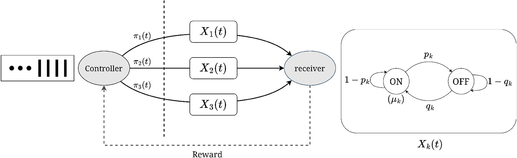
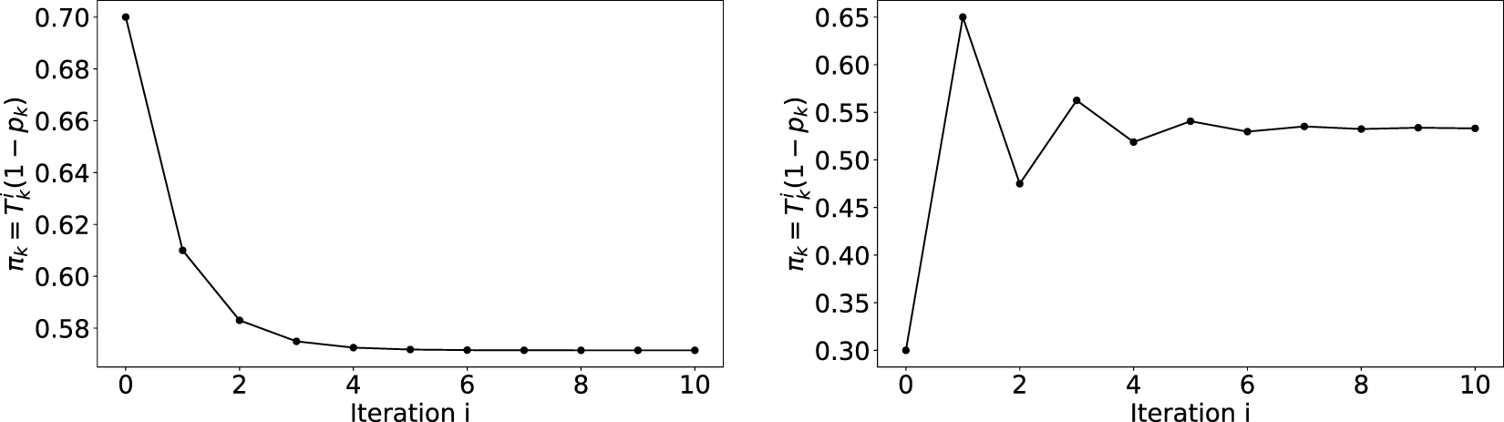


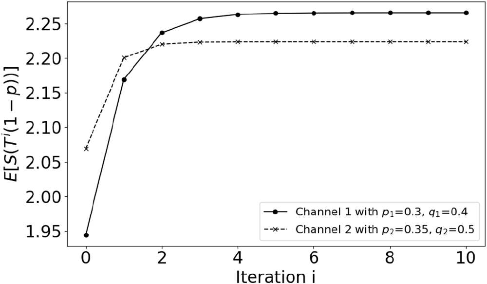


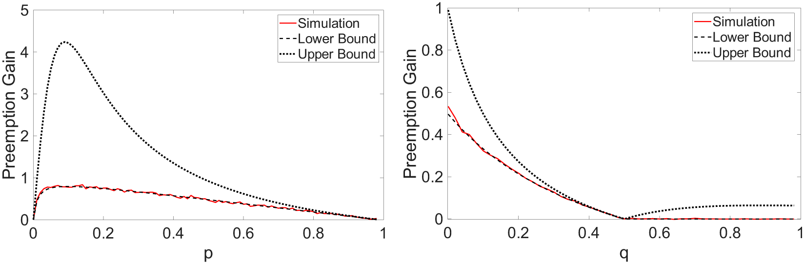


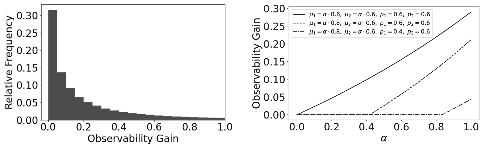


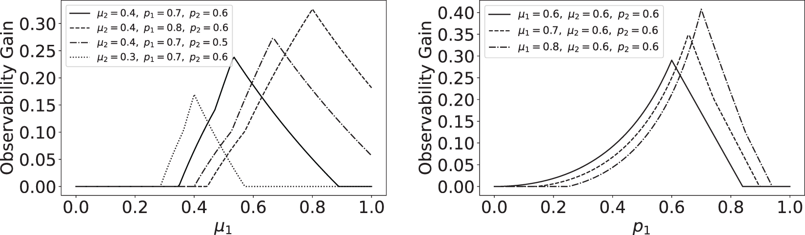


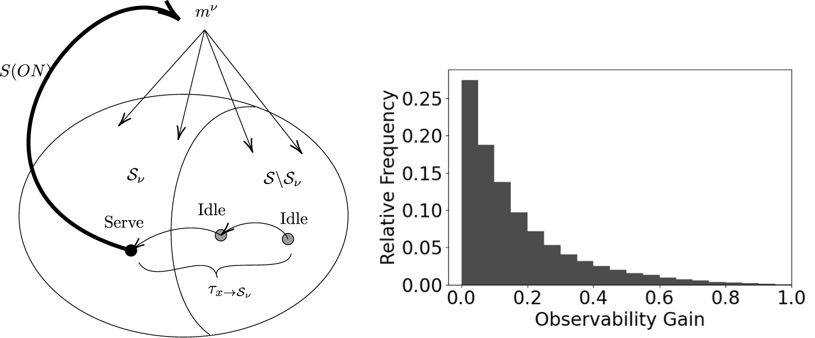
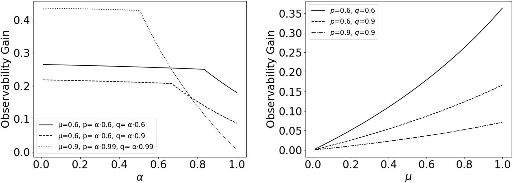


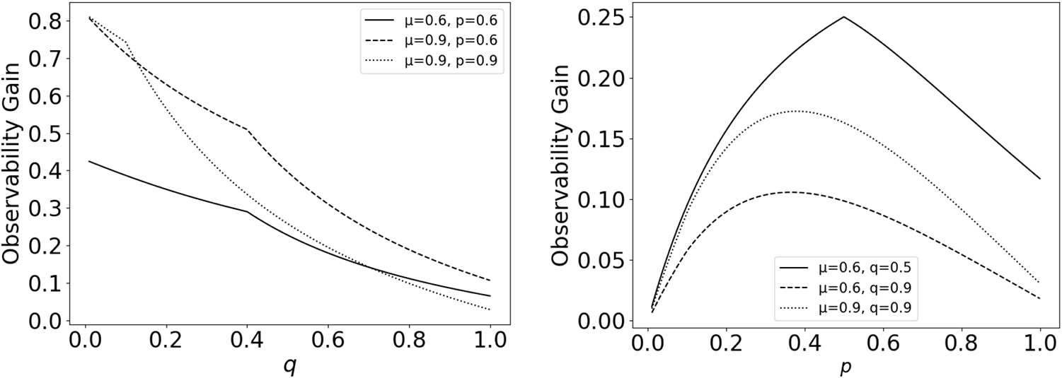


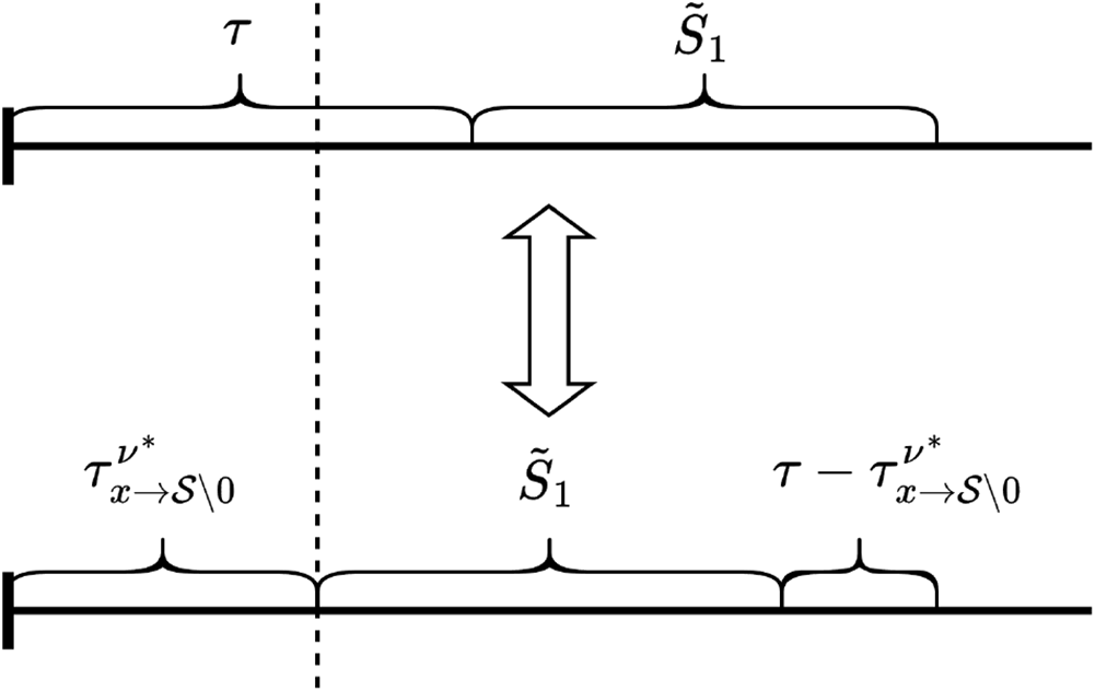

 Open access

