


1. Introduction
Understanding and modeling the interactions among input features represent a core challenge in predictive modeling on tabular data. These interactions refer to how multiple variables jointly influence the target outcome in ways that go beyond their individual, isolated effects. In many real-world cases, the relationship between predictors and the response variable is not simply additive and may involve complex interdependencies. This is particularly relevant in insurance pricing, where factors such as driver age, location, and driving behavior can interact in nonobvious ways to affect risk assessment and premium calculation. Overlooking or misspecifying such interactions can lead to suboptimal models, resulting in price distortions and potentially biased interpretations.
Traditionally, the insurance industry has relied on generalized linear models (GLMs) due to their interpretability, strong statistical foundation, and also for computational reasons; we refer to Nelder and Wedderburn (Reference Nelder and Wedderburn1972) and McCullagh and Nelder (Reference McCullagh and Nelder1983). In the GLM framework, the expected value of the response variable is modeled as a linear combination of predictors, linked to the response through a specified link function. While GLMs allow for the estimation of individual covariate effects, they offer limited capability to capture interactions among variables. In fact, interactions can be integrated, but each one needs to be engineered manually, which clearly limits their scope and the model complexity and accuracy.
Generalized additive models (GAMs) were introduced in Hastie and Tibshirani (Reference Hastie and Tibshirani1986) as an extension of GLMs relaxing the assumption of linearity see also Wood (Reference Wood2017). They allow each predictor to have a nonlinear effect on the response variable. This is accomplished by replacing the original covariates with smooth functions (typically splines) applied individually to each input variable. GAMs have often been used in the context of actuarial science as a foundation for developing more sophisticated methods to solve actuarial problems; notable examples include Chang et al. (Reference Chang, Gao and Shi2024) and Maillart and Robert (Reference Maillart and Robert2024). Building upon GAMs with Pairwise Interactions (GA
 $^2$
Ms) extend the framework by incorporating a selected set of pairwise feature interactions, see Lou et al. (Reference Lou, Caruana, Gehrke and Hooker2013). These additional components enable the model to capture the joint effects of feature pairs on the response variable. Similarly to interactions in GLMs, GA
 $^{2}$
Ms typically require manual identification and specification of interaction terms, which demands domain expertise and time-consuming feature engineering. This reliance on expert judgment can introduce subjectivity and biases, and it may make the model sensitive to the modeler’s choices, potentially affecting both predictive performance and generalization capability.
Deep neural networks (DNNs) have attracted a growing attention in actuarial science as powerful tools for predictive modeling; for an extended discussion see Richman (Reference Richman2021a,Reference Richmanb). These models can be viewed as an extension of GLMs that allow for the modeling of nonlinear relationships; see Chapter 5 of Wüthrich et al. (Reference Wüthrich, Richman, Avanzi, Lindholm, Maggi, Mayer, Schelldorfer and Scognamiglio2025). In particular, based on a successful training algorithm, DNNs perform automated feature engineering. Through the mechanism of representation learning, DNNs transform original input features into new, higher-level representations via multiple layers of nonlinear functions, which are optimized to predict the response variable. This hierarchical structure allows the model to automatically construct features that capture higher-order interactions among the original covariates. Despite their strong predictive performance, DNNs present significant challenges, particularly in identifying, quantifying and interpreting feature interactions. The complexity of the learned representations makes it difficult to understand how input variables jointly contribute to the model’s predictions. For these reasons, DNNs are sometimes called black box models.
Modern machine learning literature grapples with the challenge of effectively modeling and interpreting feature interactions within neural networks. Song et al. (Reference Song, Shi, Xiao, Duan, Xu, Zhang and Tang2019) address this issue by proposing a specialized DNN architecture designed to automatically learn feature interactions in presence of tabular data. The model employs a multi-head self-attention mechanism, inspired by the transformer architecture of Vaswani et al. (Reference Vaswani, Shazeer, Parmar, Uszkoreit, Jones, Gomez, Kaiser and Polosukhin2017), to explicitly capture interactions between features, thereby eliminating the need for manual feature engineering. Tsang et al. (Reference Tsang, Cheng and Liu2018) introduce a method for detecting statistical interactions in trained DNNs by analyzing the values of the learned weights. Li et al. (Reference Li, Cui, Wu, Zhang and Wang2019) propose modeling categorical feature interactions by representing covariates using a graph, where each node corresponds to a distinct feature field. Interactions among features are effectively captured through the propagation mechanisms of a graph neural network (GNN). Enouen and Liu (Reference Enouen and Liu2022) develop a DNNs-based approach that extends classical GAMs by introducing an additional component to capture higher-order feature interactions. Havrylenko and Heger (Reference Havrylenko and Heger2024) revisit the CANN proposal of Wüthrich and Merz (Reference Wüthrich and Merz2019) to identify the most significant interacting pairs missing in a GLM.
The contribution of this paper is to introduce the tree-like pairwise interaction network (PIN), a novel neural network architecture designed to model and identify pairwise feature interactions in tabular data. The PIN architecture embeds each input feature into a learned latent space and then explicitly models all pairwise interactions through a shared feed-forward neural network (FNN). Sharing this FNN implies an efficient way of dealing with model parameters, and to still allow for variability between the different interactions, each interaction makes use of a dedicated set of learnable parameters – playing a similar role to the classification (CLS) token used in Devlin et al. (Reference Devlin, Chang, Lee and Toutanova2018) – which is aimed at modeling the dependence structure between each pair of features. The output of each interaction is passed through a centered hard sigmoid activation function that mimics the discrete partitioning behavior of decision trees, yet in a continuous and differentiable form. This results in tree-like structures (using binary splits), and this model allows for direct inspection of interaction terms allowing for model explainability. The proposed PIN also exhibits connections with several well-established machine learning models, including gradient boosting, GA
 $^{2}$
M, and GNNs. These relationships are explored in detail throughout the manuscript. We assess the performance of the tree-like PIN on two widely studied datasets, the French motor third-party liability (MTPL) claims frequency dataset and the Belgian MTPL dataset, both available from of Dutang et al. (Reference Dutang, Charpentier and Gallic2024). Our experiments demonstrate that the PIN architecture delivers strong predictive accuracy in terms of Poisson losses, outperforming not only classical benchmarks but also more recent neural network architectures, such as the credibility transformer introduced by Richman et al. (Reference Richman, Scognamiglio and Wüthrich2025). Moreover, unlike most other network architectures, the PIN architecture allows for an efficient computation of SHapley’s Additive exPlanations (SHAP). The crucial point is that the PIN architecture only involves pairwise interactions, and it has been shown in Lundberg (Reference Lundberg2018) and Mayer and Wüthrich (Reference Mayer and Wüthrich2025, Proposition 3.1) that this allows for a very efficient computation of the Shapley values using paired permutation SHAP sampling.
Concluding this introduction: Our novel architecture of the tree-like PIN provides superior performance on tabular data over currently used network architectures, and at the same time, it provides explainability. We believe that this makes the tree-like PIN an interesting proposal for actuarial pricing.
The paper is organized as follows. In Section 2, we introduce the PIN architecture, starting with feature embeddings and proceeding through the PIN. Section 3 details the application of the PIN to claims frequency modeling. In Section 4.1, we propose interaction importance measures for model interpretation, and we illustrate how the SHAP explanation can be computed within the PIN architecture using paired-sampling permutation SHAP. In Section 5, we study a second real-world dataset to confirm the excellent predictive performance of the PIN proposal. Finally, Section 6 concludes with a summary and future research directions.
2. Tree-like pairwise interaction network
2.1 Feature embedding
We start from tabular input data
 $\boldsymbol{x}=(x_1,\ldots , x_q)^\top$
. In a first step, we tokenize this tabular input data to an input tensor
 $\boldsymbol{\phi }=\boldsymbol{\phi }(\boldsymbol{x})= [\phi _1,\ldots , \phi _q ] \in {\mathbb R}^{d \times q}$
; this step is done in complete analogy to Gorishniy et al. (Reference Gorishniy, Rubachev, Khrulkov and Babenko2021), Brauer (Reference Brauer2024), and Richman et al. (Reference Richman, Scognamiglio and Wüthrich2025). For this first step, we select a fixed embedding dimension
 $d \in {\mathbb N}$
; this is a hyperparameter selected by the modeler.
Categorical features.
For categorical feature components
 $x_j\in \mathcal{X}_j=\{1,\ldots , n_j\} \subset {\mathbb N}$
, having
 $n_j$
levels, consider a
 $d$
-dimensional entity embedding
 $\phi _j\,:\, \mathcal{X}_j \to {\mathbb R}^d$
 \begin{equation} x_j \,\mapsto \,\phi _j(x_j) = \sum _{k=1}^{n_j} W^{(0)}_{j,k} \,\unicode{x1D7D9}_{\{x_j=k\}}, \end{equation}
where
 $W^{(0)}_j=[W^{(0)}_{j,1}, \ldots , W^{(0)}_{j,n_j}]^\top \in {\mathbb R}^{n_j \times d}$
is an embedding matrix, which is a learnable parameter.
Continuous features.
For continuous feature components
 $x_j \in {\mathbb R}$
, we consider a
 $d$
-dimensional FNN embedding
 $\phi _j\,:\, {\mathbb R} \to {\mathbb R}^d$
 \begin{equation} x_j \,\mapsto \,\phi _j(x_j) = W^{(2)}_j \,\tanh \left (W^{(1)}_j x_j + b^{(1)}_j\right ) + b^{(2)}_j \end{equation}
with biases
 $b^{(1)}_j \in {\mathbb R}^{d'}$
and
 $b^{(2)}_j \in {\mathbb R}^d$
, weight matrices
 $W^{(1)}_j \in {\mathbb R}^{d' \times 1}$
and
 $W^{(2)}_j \in {\mathbb R}^{d \times d'}$
, for a fixed number of units
 $d'$
, and where the hyperbolic tangent function is applied element-wise.
Collecting all embedded components
 $(\phi _j)_{j=1}^q=(\phi _j(x_j))_{j=1}^q$
of the input
 $\boldsymbol{x}$
gives us the tensor
 \begin{equation} \boldsymbol{\phi }=\boldsymbol{\phi }(\boldsymbol{x})= [\phi _1,\ldots , \phi _q ]= [\phi _1(x_1),\ldots , \phi _q(x_q) ] \in {\mathbb R}^{d \times q}. \end{equation}
This tensor
 $\boldsymbol{\phi }$
involves the embedding weights
 $W^{(0)}_j \in {\mathbb R}^{n_j \times d}$
from the categorical features (of dimension
 $n_jd$
), and the FNN biases and weights
 $(b^{(1)}_j, b^{(2)}_j , W^{(1)}_j, W^{(2)}_j)$
from the continuous feature embeddings (of dimension
 $2 d' + (d'+1)d$
). All these biases and weights are learned from the available training data.
The categorical entity embeddings (2.1) and the continuous feature embeddings (2.2) do not necessarily live on the same scale. If a common scale is desired, this can be achieved either through ridge regularization or by applying separate normalization layers to the two types of embeddings. In our examples, the embeddings are not directly extracted, but they are further processed by interaction tokens introduced in the next section. These interaction tokens alleviate the potential scale discrepancies. Therefore, we do not regularize or normalize the embeddings.
2.2 Pairwise interaction layer
The tensor
 $\boldsymbol{\phi }=\boldsymbol{\phi }(\boldsymbol{x})$
, given in (2.3) and containing the tokens
 $(\phi _j(x_j))_{j=1}^q$
, is expressing the individual feature components of
 $\boldsymbol{x} \in \mathcal{X}$
before they have been interacting with each other. In the next step, we are going to let these tokens interact in a pairwise manner. This can be interpreted in a similar way as the query–key interaction concept in the attention layer of Vaswani et al. (Reference Vaswani, Shazeer, Parmar, Uszkoreit, Jones, Gomez, Kaiser and Polosukhin2017).
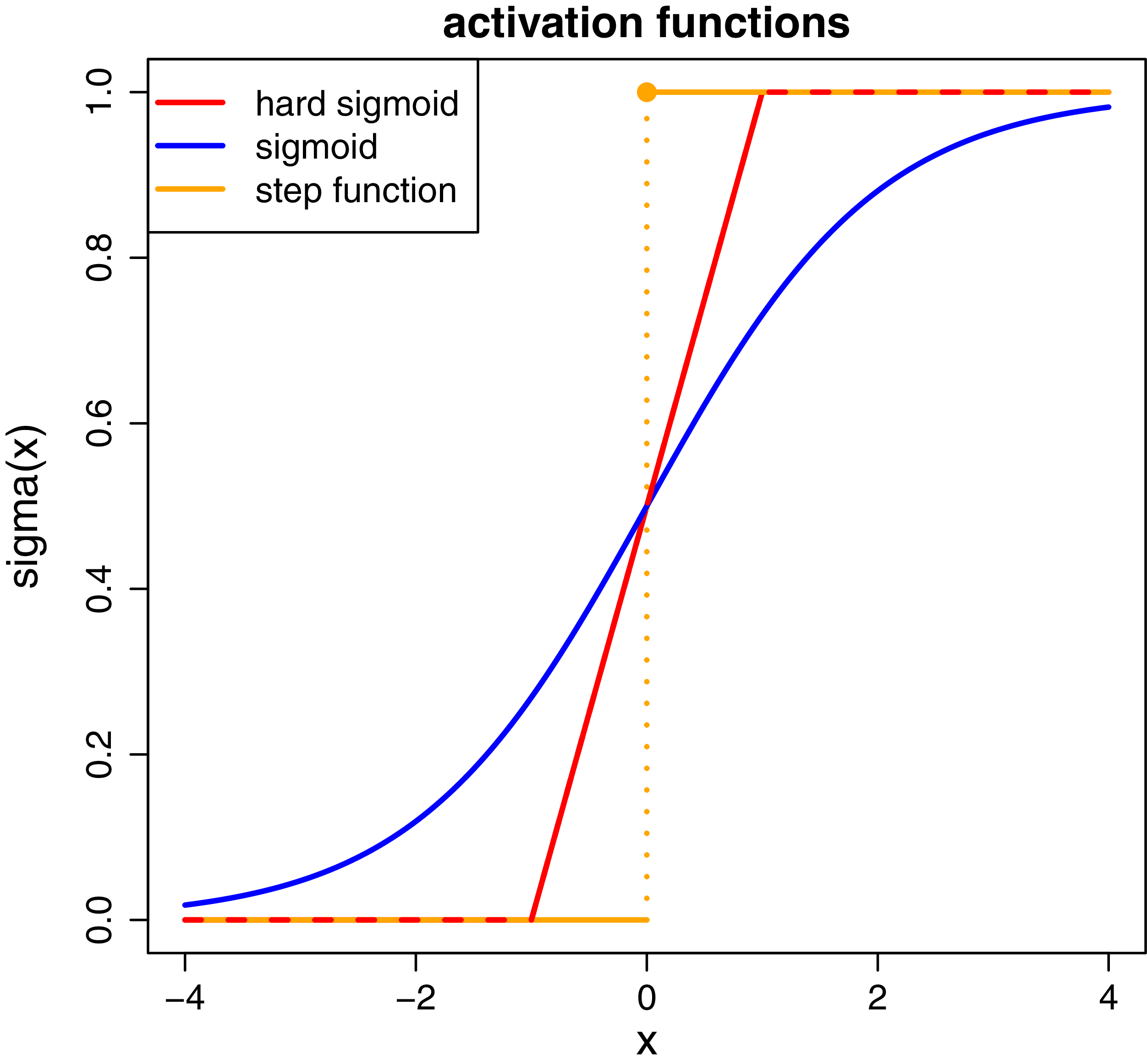
We recall the (centered version of the) hard sigmoid activation
 \begin{equation} \sigma _{\textrm {hard}} \,:\,{\mathbb R} \to [0,1], \qquad x\,\mapsto \,\sigma _{\textrm {hard}}(x) = \max \left (0, \,\min \left (1, \, \frac {1+x}{2}\right )\right ). \end{equation}
This is the centered version of the hard sigmoid activation; there is also a noncentered version with
 $(1+x)/2$
being replaced by
 $x$
in (2.4). The centered version is directly comparable to the sigmoid activation function and the step function activation, see Figure 1.
Activation functions: (centered) hard sigmoid, sigmoid, and step function.

We now let
 $\phi _j$
and
 $\phi _k$
interact,
 $j \le k$
. To support these interactions, we introduce interaction tokens
 $\boldsymbol{e}_{j,k} \in {\mathbb R}^{d_0}$
, for a given hyper-parameter
 $d_0 \in {\mathbb N}$
. The tokens consist of a set of learnable parameters that are optimized jointly with the rest of the model during network training. Before interacting, these tokens do not encode any information and are randomly initialized, like the other network parameters. This is analogous to the CLS token used in Devlin et al. (Reference Devlin, Chang, Lee and Toutanova2018) and Richman et al. (Reference Richman, Scognamiglio and Wüthrich2025). After training, the tokens are calibrated to support pairwise interactions between the
 $j$
-th and
 $k$
-th covariates. We concatenate the three vectors to a row-vector
 $(\phi _j, \phi _k, \boldsymbol{e}_{j,k})^\top \in {\mathbb R}^{2d+d_0}$
,
 $j \le k$
. The goal of the interaction tokens is to learn the interaction structure within the tensor
 $\boldsymbol{\phi }$
for predicting the response
 $Y$
, in particular, different pairs
 $(\phi _j, \phi _k)$
may have a different interaction behavior which is reflected in different learned interaction tokens
 $\boldsymbol{e}_{j,k}$
,
 $j \le k$
. Unlike the CLS token of Devlin et al. (Reference Devlin, Chang, Lee and Toutanova2018) and Richman et al. (Reference Richman, Scognamiglio and Wüthrich2025), we do not use these interaction tokens to strip out information, but we add them to allow for the necessary modeling flexibility to be able to account for differences in the different interaction pairs.
Define the shared interaction network
 $f_\theta \,:\,{\mathbb R}^{2d+d_0} \to {\mathbb R}$
as a composition of three FNN layers
 \begin{equation} f_\theta (\phi _j, \phi _k, \boldsymbol{e}_{j,k}) = W^{(3)} \,\textrm {ReLU}\big (W^{(2)} \,\textrm {ReLU}\big (W^{(1)} (\phi _j, \phi _k, \boldsymbol{e}_{j,k})^\top + b^{(1)}\big ) + b^{(2)}\big ) + b^{(3)}, \end{equation}
with:
-
• the 1st FNN layer has
 $d_1$
units, rectified linear unit (ReLU) activation, network weights
$W^{(1)}\in {\mathbb R}^{d_1 \times (2d+d_0)}$
, and bias
$b^{(1)}\in {\mathbb R}^{d_1}$
;
-
• the 2nd FNN layer has
$d_2$
units, ReLU activation, network weights
$W^{(2)}\in {\mathbb R}^{d_2 \times d_1}$
, and bias
$b^{(2)}\in {\mathbb R}^{d_2}$
; -
• the output layer has
$1$
unit, linear activation, network weights
$W^{(3)}\in {\mathbb R}^{1 \times d_2}$
, and bias
$b^{(3)}\in {\mathbb R}$
;


and
 $\theta =(W^{(1)},b^{(1)}, W^{(2)},b^{(2)}, W^{(3)},b^{(3)})$
collects all network parameters. This interaction network
 $f_\theta$
is going to be shared by all pairwise interactions between the components of
 $\boldsymbol{\phi }$
, i.e., there is one single network parameter
 $\theta$
that is shared by all ordered pairs
 $(\phi _j,\phi _k)$
,
 $1\le j \le k \le q$
. This can also be seen as a so-called time-distributed network as being used, e.g., in recurrent neural networks. To differentiate different forms of interactions of the different ordered pairs,
 $j \le k$
, we let the interaction tokens
 $\boldsymbol{e}_{j,k}$
learn the pairwise interaction structures.
Definition 2.1 (pairwise interaction layer). For feature tokens
 $\phi _j({\cdot} )$
and
 $\phi _k({\cdot} )$
,
 $1\le j \le k \le q$
, and interaction tokens
 $\boldsymbol{e}_{j,k}$
, we define the pairwise interaction units by
 \begin{equation} h_{j,k}(\boldsymbol{x}) = \sigma _{\mathrm {hard}} (f_\theta (\phi _j(x_j), \phi _k(x_k), \boldsymbol{e}_{j,k} ) )\,\in \,[0,1]. \end{equation}
The pairwise interaction layer for
 $\boldsymbol{x} \in \mathcal{X}$
is defined by the upper-right triangular matrix
 \begin{equation} \left (h_{j,k}(\boldsymbol{x})\right )_{1\le j \le k \le q} = \begin{pmatrix} h_{1,1}(\boldsymbol{x}) & h_{1,2}(\boldsymbol{x}) & \cdots & h_{1,q-1}(\boldsymbol{x})& h_{1,q}(\boldsymbol{x})\\ \mathrm {n/a} & h_{2,2}(\boldsymbol{x}) & \cdots & h_{2,q-1}(\boldsymbol{x})& h_{2,q}(\boldsymbol{x})\\ \vdots &\vdots &\ddots &\vdots &\vdots &\\ \mathrm {n/a} & \mathrm {n/a} & \cdots & h_{q-1,q-1}(\boldsymbol{x})& h_{q-1,q}(\boldsymbol{x})\\ \mathrm {n/a} & \mathrm {n/a} & \cdots & \mathrm {n/a} & h_{q,q}(\boldsymbol{x}) \end{pmatrix} , \end{equation}
where the lower-left part is undefined indicated by n/a.
We remark that the diagonal entries represent the “self-interaction” of each covariate component and can be interpreted as the corresponding individual (main) effects. Including these diagonal terms allows the model to learn nonlinear functions that capture the marginal contribution of each variable, while preserving the same unified representation used for modeling pairwise interactions.
Example 2.2. We give a simple example of the pairwise interaction layer. We assume only continuous features, that is,
 $\boldsymbol{x} \in {\mathbb R}^q$
. We select one-dimensional linear feature embeddings (tokenization)
 $x_j \mapsto \phi _j(x_j)=x_j$
for all
 $1\le j \le q$
. This gives us the tensor
 $\boldsymbol{\phi } = \boldsymbol{\phi }(\boldsymbol{x})=\boldsymbol{x} \in {\mathbb R}^{1 \times q}$
. For the shared interaction network
 $f_\theta$
, we select a simple additive function and the interaction tokens are set off in this example. This gives the simplified version
 \begin{equation} h^{\mathrm {add}}_{j,k}(\boldsymbol{x}) = \sigma _{\mathrm {hard}}(x_j+x_k)\qquad \text{ for $j\le k$.} \end{equation}
This is illustrated on the left-hand side of Figure 2 for
 $j\lt k$
.
The right-hand side of Figure 2 shows a linear additive interaction network with the first component
 $x_j$
being scaled with
 $1/3$
. We note that these linear additive interaction networks are rather similar to binary decision tree partitions of the feature space. We allow for additional flexibility by letting the interaction network
 $f_\theta$
be nonlinear and by letting the interaction token
 $\boldsymbol{e}_{j,k}$
learn different pairwise interaction structures. It is precisely this ability to learn to modify the inputs that gives the pairwise interaction layers their power.
Interaction layers: (lhs)
 $\sigma _{\mathrm {hard}}(x_j+x_k)$
and (rhs)
 $\sigma _{\mathrm {hard}}(x_j/3+x_k)$
for
 $j\lt k$
.

2.3 Pairwise interaction network
We are now ready to define the tree-like PIN.
Definition 2.3.
Choose an output activation function
 $g$
. The PIN) is defined by
 $f_{\mathrm {PIN}}\,:\,\mathcal{X} \to {\mathbb R}$
 \begin{equation} \boldsymbol{x} \,\mapsto \, f_{\mathrm {PIN}}(\boldsymbol{x}) = g\left (\sum _{1\le j \le k \le q} w_{j,k} \, h_{j,k}(\boldsymbol{x})+b\right )\!, \end{equation}
with learnable (real-valued) output weights
 $(w_{j,k})_{1\le j \le k \le q}$
and bias
 $b \in {\mathbb R}$
.
There is structural similarity between a PIN and a classical gradient boosting machine (GBM)
 \begin{equation*} f_{\mathrm {GBM}}(\boldsymbol{x}) = \sum _{m=1}^M \sum _{l=1}^L \gamma _{m,l}\, \unicode {x1D7D9}_{R_{m,l}}(\boldsymbol{x}), \end{equation*}
with
 $M\in {\mathbb N}$
GBM iterations considering binary split decision trees with
 $L$
leaves giving the partition
 $(R_{m,l})_{l=1}^L$
of the feature space
 $\mathcal{X}$
and assigning the leaf values
 $(\gamma _{m,l})_{l=1}^L$
to this partition. We start by discussing the structural correspondence between the two regression functions.

We list some key differences:
-
1. Smooth activation: The hard binary decisions
$\unicode{x1D7D9}_{R_{m,l}}(\boldsymbol{x})$
are replaced by continuous functions involving the hard sigmoid function. -
2. Learned representations: There is an automatic feature transformations through embeddings resulting in the tensor
$\boldsymbol{\phi }$
, whereas GBMs split on the original feature values. -
3. Parameter sharing: Common network
$f_\theta$
across all interactions, and the interaction tokens learn the differences between the pairwise interactions
$(\phi _j,\phi _k)$
. -
4. Joint optimization: All components trained simultaneously, where as the GBM learns the parameters recursively in stage-wise adaptive way.


The other close connection of the PIN is to a GA
 $^{2}$
M. A GA
 $^{2}$
M is obtained from a GAM by adding interaction terms to the regression function
 \begin{equation} g^{-1}\left (\mu (\boldsymbol{X})\right ) = b+\sum _{j=1}^q f_j(X_j) + \sum _{1\le j\lt k \le q} f_{j,k}(X_j,X_k), \end{equation}
where
 $f_j$
and
 $f_{j,k}$
are selected from a given class of splines; see Lou et al. (Reference Lou, Caruana, Gehrke and Hooker2013). A classical GAM only considers the terms
 $(f_j)_{j=1}^q$
, and the GA
 $^{2}$
M adds the pairwise interaction terms
 $(f_{j,k})_{1\le j\lt k \le q}$
. We note that this GA
 $^{2}$
M (2.10) has the same structure as our PIN (2.9), the difference is that we replace the splines
 $(f_j)_{j=1}^q$
and
 $(f_{j,k})_{1\le j\lt k \le q}$
by pairwise interaction layers
 $(h_{j,k})_{1\le j\le k \le q}$
being based on FNNs.
2.4 Connection to graph neural networks
The pairwise interaction structure of the PIN can be naturally interpreted through the lens of GNNs. We formalize this connection and demonstrate how our model can be viewed as a special case of message passing on a complete graph with learned edge features.
Definition 2.4 (feature graph). For input
 $\boldsymbol{x} \in \mathcal{X}$
, we define the corresponding feature graph
 $G_{\boldsymbol{x}} = (V, E)$
as follows:
-
• Vertices
$V = \{1,\ldots , q\}$
correspond to feature components;
-
• Edges
$E = \{(j,k) \,:\,1 \leq j \le k \leq q\}$
form a complete graph;
-
• Node features
$\phi _j = \phi _j(x_j) \in {\mathbb R}^d$
for
$j \in V$
; -
• Edge features
$\boldsymbol{e}_{j,k} \in {\mathbb R}^{d_0}$
for
$(j,k) \in E$
.


Our PIN can be reformulated as a message passing neural network with a single update step.
Definition 2.5 (message function). The message function
 $\mathcal{M}\,:\,{\mathbb R}^d \times {\mathbb R}^d \times {\mathbb R}^{d_0} \to {\mathbb R}$
is defined as
 \begin{equation*} \mathcal{M}(\phi _j, \phi _k, \boldsymbol{e}_{j,k}) = \sigma _{\mathrm {hard}}(f_\theta (\phi _j, \phi _k, \boldsymbol{e}_{j,k})), \end{equation*}
where
 $f_\theta$
is the shared interaction network
(2.5)
.
It is obvious that the PIN (2.9) is equivalent to the GNN defined by
 \begin{equation*} f_{\mathrm {GNN}}(\boldsymbol{x}) = g\left (\sum _{(j,k) \in E} w_{j,k}\, \mathcal{M}(\phi _j, \phi _k, \boldsymbol{e}_{j,k})\right )\!. \end{equation*}
Our architecture differs from traditional GNNs in the following ways:
-
1. Edge-centric: While most GNNs focus on learning node representations, our model primarily focuses on edge interactions and the interaction token
$\boldsymbol{e}_{j,k}$
to distinguish different interaction patterns. -
2. Learned edge features: The interaction tokens
$\boldsymbol{e}_{j,k}$
are learned parameters rather than derived features. -
3. Single-pass architecture: Unlike typical GNNs that use multiple layers of message passing, our model uses a single pass with a more expressive message function.
-
4. Bounded messages: The hard sigmoid activation ensures bounded message values, similar to the binary nature of GBM binary decision tree splits.


Having this connection to GNNs provides the following additional theoretical insights.
Proposition 2.6 (permutation invariance). For any permutation
 $\pi$
of the feature indices, the model output is invariant up to a reindexing of the output weights
 $w_{j,k}$
.
This proposition immediately follows by analyzing permutations of the components/vertices
 $V=\{1,\ldots , q\}$
.
Proposition 2.7 (expressiveness). The PIN can express any message-passing GNN with binary messages, single-layer architecture and complete graph structure.
Using GNN operations, the GNN perspective suggests several natural extensions to our base model.
Definition 2.8 (multi-layer PIN). We can define a
 $K$
-layer model through iterative message passing, that is,
 \begin{equation} \phi _v^{(k+1)} = \operatorname {UPDATE}\left (\phi _v^{(k)}, \sum _{u \in \mathcal{N}(v)} \mathcal{M}^{(k)}\big(\phi _u^{(k)}, \phi _v^{(k)}, \boldsymbol{e}_{u,v}\big)\right ) \end{equation}
where
 $\phi _v^{(0)} = \phi _v(x_v)$
,
 $v \in V$
,
 $k = 0,\ldots ,K-1$
, and
 $\mathcal{N}(v)$
are the vertices adjacent to
 $v$
. The
 $\operatorname {UPDATE}$
can be various functions such as the maximum or the mean of the two components.
Remark 2.9 (attention mechanism). The model can be enhanced with an attention mechanism by replacing the fixed output weights
 $w_{j,k}$
with learned functions of the node features
 \begin{equation*} w_{j,k} = \alpha _\vartheta (\phi _j, \phi _k), \end{equation*}
where
 $\alpha _\vartheta$
is a (self-)attention layer with parameters
 $\vartheta$
; see Vaswani et al. (Reference Vaswani, Shazeer, Parmar, Uszkoreit, Jones, Gomez, Kaiser and Polosukhin2017). If we apply the attention weights only to pairs
 $j\lt k$
, and if we apply a thresholding, we obtain
 \begin{equation} \boldsymbol{x} \,\mapsto \, g\left (b+\sum _{j=1}^k w_{j} \, h_{j,j}(\boldsymbol{x})+\sum _{1\le j \lt k \le q} \mathrm {ReLU} (\alpha _\vartheta (\phi _j, \phi _k)-\tau )\, h_{j,k}(\boldsymbol{x})\right ), \end{equation}
for an attention threshold
 $\tau \in {\mathbb R}$
. The thresholding in (2.12) gives a natural way of pairwise interaction selection.
The connection to GNNs not only provides theoretical insights but also suggests practical extensions and implementation strategies for the PIN architecture. Moreover, for efficient implementations, existing GNN libraries are available that allow for batched processing (graph batching for parallel processing), optimized GNN kernels on GPUs, and optional sparsification of the interaction graph, similar to (2.12).
3. Claims frequency example
We present a first example that we take in several steps to illustrate the functioning of the tree-like PIN. We consider the popular French MTPL claims frequency dataset available from Dutang et al. (Reference Dutang, Charpentier and Gallic2024). We apply the same data cleaning procedure as described in Wüthrich and Merz (Reference Wüthrich and Merz2023);Footnote 1 for a detailed discussion of the French MTPL dataset, we refer to Appendix B of the latter reference.
Our goal is to predict the MTPL claims frequencies
 $Y_i=N_i/v_i$
of the insurance policyholders
 $i\in \{1,\ldots , n\}$
, where
 $N_i$
is the number of claims of policyholder
 $i$
,
 $v_i\gt 0$
is the time exposure (in yearly units) of that policyholder, and
 $\boldsymbol{x}_i$
describes their features. We fit different tree-like PINs to this data by using the Poisson deviance (PD) loss as the objective function; the PD loss is the canonical strictly consistent loss function choice for mean estimation for claims count problems in insurance; Gneiting and Raftery (Reference Gneiting and Raftery2007) and Wüthrich et al. (Reference Wüthrich, Richman, Avanzi, Lindholm, Maggi, Mayer, Schelldorfer and Scognamiglio2025). For given learning data
 $\mathcal{L}=(Y_i, \boldsymbol{x}_i, v_i)_{i=1}^n$
, we aim at minimizing the following (average) PD loss to find the optimal weights of the tree-like PIN
 \begin{equation} L_{\mathrm {PD}}( \mathcal{L}, f_{\mathrm {PIN}}) = \frac {1}{n} \left [ \sum _{i:\,Y_i=0} 2v_i\,f_{\mathrm {PIN}}(\boldsymbol{x}_i) \;+\; \sum _{i:\,Y_i\neq 0} 2v_i\left (f_{\mathrm {PIN}}(\boldsymbol{x}_i)-Y_i- Y_i \log \left (\frac {f_{\mathrm {PIN}}(\boldsymbol{x}_i)}{Y_i}\right )\right ) \right ]\!, \end{equation}
where
 $f_{\mathrm {PIN}}({\cdot} )$
is the PIN given in (2.9), and we select the exponential output function
 $g({\cdot} )=\exp ({\cdot} )$
, which is the canonical link of the Poisson model.
For model training (minimizing the PD loss
 $L_{\mathrm {PD}}$
in the network weights and biases), we use the Adam optimizer on batches of size 128, with an initial learning rate of 0.001. We then apply a learning rate reduction on plateau (factor 0.9, patience 5), and early stopping is exercised based on a 10% validation set of the learning data
 $\mathcal{L}$
; the size of the learning data is
 $n=610,206$
. Moreover, we hold an independent test sample
 $\mathcal{T}=(Y_j, \boldsymbol{x}_j, v_j)_{j=1}^m$
of sample size
 $m=67,801$
, that is going to be used for out-of-sample model testing and model comparison. The learning and test samples,
 $\mathcal{L}$
and
 $\mathcal{T}$
, are identical to Brauer (Reference Brauer2024) and Richman et al. (Reference Richman, Scognamiglio and Wüthrich2025), which makes all results directly comparable to these references.
The case of a linear PIN, with two continuous features only.
Similar to Example 2.2, we start with a linear PIN, and we only consider the two continuous features “driver age” (DrivAge) and “log-Density”. Moreover, we only consider the interaction term
 $h_{1,2}(\boldsymbol{x})$
and we drop the diagonal terms
 $h_{1,1}(\boldsymbol{x})$
and
 $h_{2,2}(\boldsymbol{x})$
by setting
 $w_{1,1}=w_{2,2}=0$
. This allows us to nicely illustrate the results. For this linear off-diagonal PIN, we select the (single,
 $q=2$
) pairwise interaction
 \begin{equation*} h^{\mathrm {linear}}_{1,2}(\boldsymbol{x}) = \sigma _{\mathrm {hard}}\big (W^{(1)}(x_1,x_2, \boldsymbol{e}_{1,2})^\top + b^{(1)}\big ). \end{equation*}
This only considers the most inner operation of the shared interaction network (2.5), with embedding dimension
 $d=1$
, interaction token dimension
 $d_0=1$
and output dimension
 $d_1=1$
. This gives us a weight matrix
 $W^{(1)}\in {\mathbb R}^{1 \times 3}$
and a bias
 $b^{(1)} \in {\mathbb R}$
. This is similar to the additive interaction (2.8), but additionally allowing for an affine transformation. Note that in this example of only one interaction pair (“DrivAge”, “log-Density”), the interaction token
 $\boldsymbol{e}_{1,2}$
would not be necessary. By inserting this linear interaction network into the PIN in (2.9) gives us a first illustrative example.
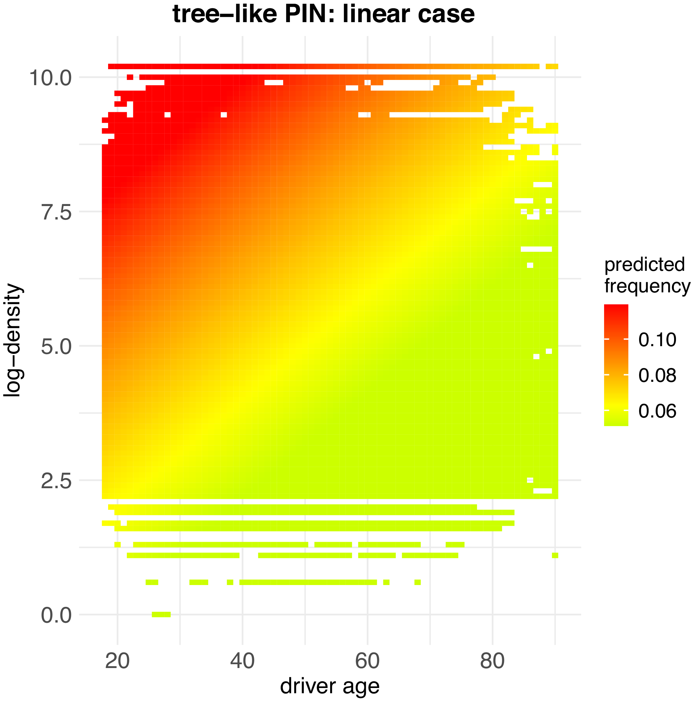
Heatmap of predicted frequencies of the linear off-diagonal PIN only considering the features “DrivAge” and “log-density”.

We fit this linear off-diagonal PIN to the learning data
 $\mathcal{L}$
using the PD loss (3.1), and the result is presented in Figure 3. The colored dots show the estimated frequencies on the insurance portfolio (for the white parts there are no insurance policies available for these feature combinations). We observe that this 1-dimensional (
 $d=1$
) linear off-diagonal PIN suggests a diagonal pattern. Related to decision trees, this corresponds to a feature space partition along the diagonal (for driver age and log-density scaled as in Figure 3). In the next example, we are going to refine this prediction by allowing for more general functional forms.
Tree-like PIN, with two continuous features only.
In our next example, we consider the non-linear tree-like PIN as introduced in (2.9). To improve the modeling step-by-step on the previous example, we again only consider the two features “DrivAge” and “log-Density” and we let them interact nonlinearly, and again we only consider the off-diagonal interaction term
 $h_{1,2}(\boldsymbol{x})$
by setting
 $w_{1,1}=w_{2,2}=0$
. We start with the 1-dimensional embedding case
 $d=1$
, thus, we consider 1-dimensional FNN embeddings
 $x_j \mapsto \phi _j(x_j) \in {\mathbb R}$
, which we then let interact by the interaction network as defined in (2.5); note that because we only have two features in this example,
 $j \in \{1, 2\}$
, this network is not shared by different interactions and the interaction token is not necessary.
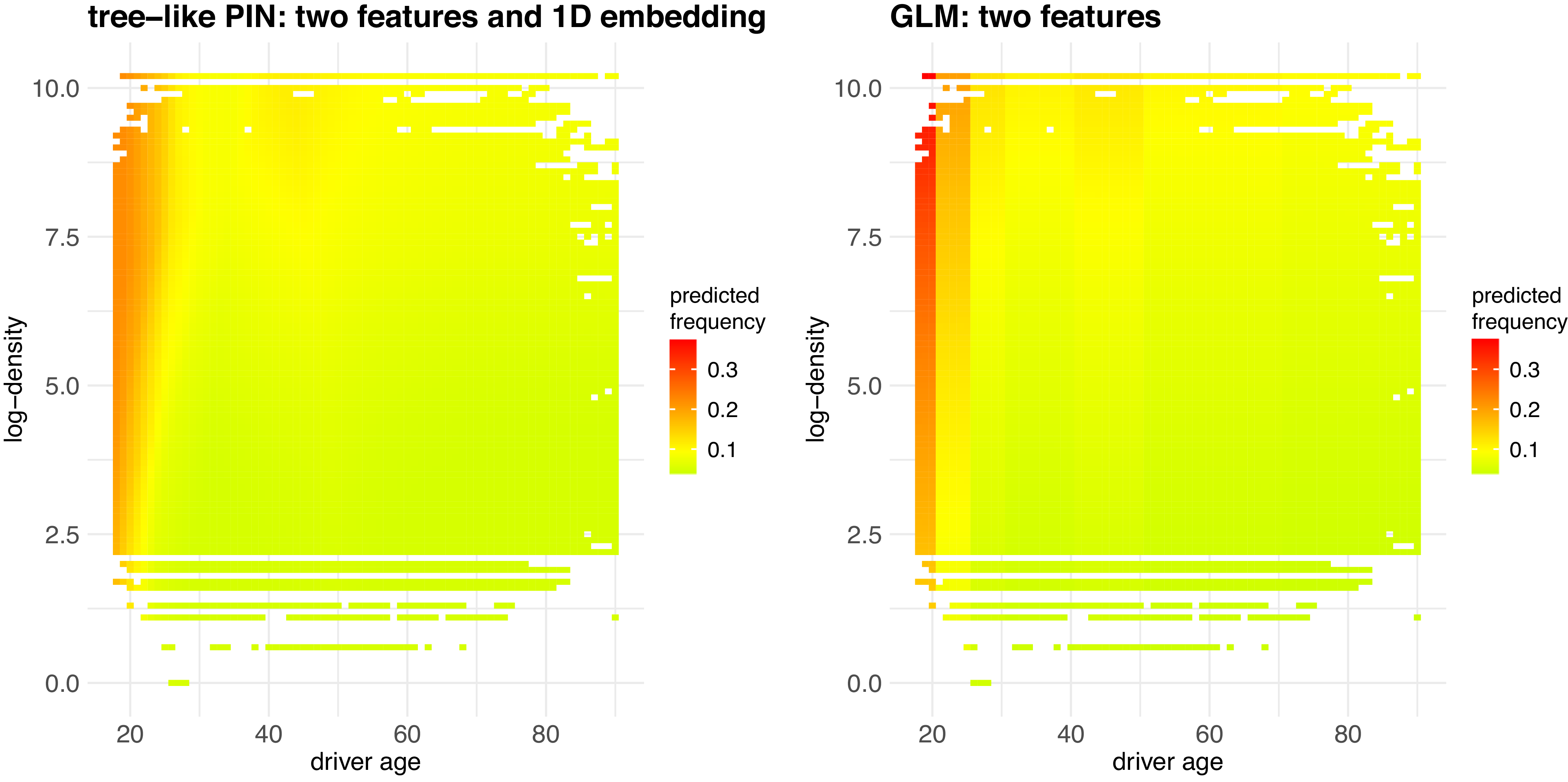
Heatmaps of predicted frequencies of (lhs) the off-diagonal PIN with 1D embedding (
 $d=1$
), and (rhs) GLM only considering the two features “DrivAge” and “log-density”.

We fit this (non-linear) off-diagonal PIN as described above by using the Adam optimizer and early stopping. The result of this 1-dimensional case with two feature components is shown in Figure 4 (lhs), and it is compared to a GLM considering the same two features “DrivAge” and “log-Density”, the first variable is encoded categorically and the second one continuously in this GLM, see Wüthrich and Merz (Reference Wüthrich and Merz2023, Section 5.2.4) for more details. The GLM in the right-hand side of Figure 4 shows a multiplicative structure in the two feature components (because of the log-link choice), and the PIN on the left-hand side gives a refinement indicating that the vertical age class coloring of the GLM is not fully appropriate. From these two plots, we also observe that the expected frequency is non-monotone in the age of driver variable.
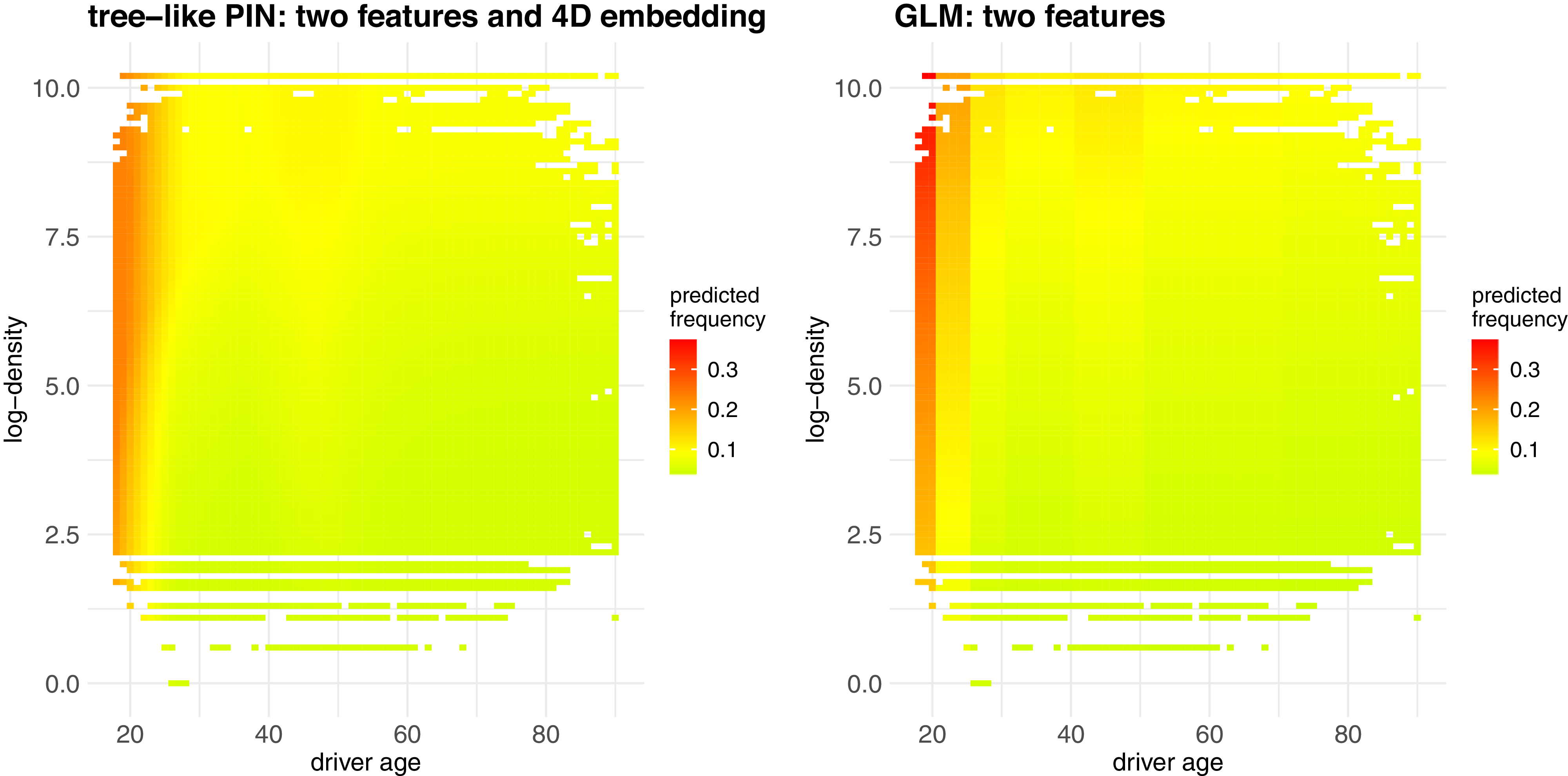
Heatmaps of predicted frequencies of (lhs) the off-diagonal PIN with 4D embedding (
 $d=4$
), and (rhs) GLM only considering the two features “DrivAge” and “log-density”.

In a next step, a further refinement is received by increasing the dimension of the embedding to
 $d=4$
in
 $x_j \mapsto \phi _j(x_j) \in {\mathbb R}^d$
. Similarly to GBMs, this overlaps multiple tree-like structures. Figure 5 (lhs) shows the resulting fitted off-diagonal PIN, which looks like a refinement of the GLM on the right-hand side, also more clearly reflecting the expected frequency increase in the driver age bucket between 40 and 50. Note that this age bucket has not been indicated to the PIN, but this finding of a higher frequency in this age bucket is purely data driven. Out-of-sample on the test data
 $\mathcal{T}$
, the PIN has a slightly better performance than the GLM w.r.t. the PD loss; we do not show the figures because in this example we only showcased the functioning of the tree-like PIN on two feature components and only in the off-diagonal case (
 $w_{1,1}=w_{2,2}=0$
); the general case is presented next.
Tree-like PIN on all feature components.
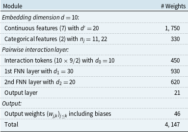
We now include all available feature components and we also consider the diagonal elements of the pairwise interaction layer (2.7). There are seven continuous and binary input variables to which we apply separate network embeddings (2.2), and two categorical variables to which we apply two entity embeddings (2.1). We select a hidden layer of dimension
 $d'=20$
in (2.2), and an entity embedding dimension of
 $d=10$
. Regarding the binary input variables, in a standard GLM framework, treating them as dummy coded factors or as continuous covariates is equivalent. In deep learning models, binary variables are often incorporated directly as continuous inputs. This parameterization yields in our case
 $2d'+(d'+1)d=250$
parameters. By contrast, using entity embeddings would require only
 $2d=20$
parameters. Therefore, if model complexity is a concern, the embedding-based approach is preferable.
This gives us a tensor
 $\boldsymbol{\phi }=\boldsymbol{\phi }(\boldsymbol{x}) \in {\mathbb R}^{10 \times 9}$
, and in total
 $10\times 9/2=45$
interaction tokens
 $\boldsymbol{e}_{j,k} \in {\mathbb R}^{10}$
,
 $1\le j \le k \le 9$
; we select dimension
 $d_0=10$
for the interaction tokens. The interaction tokens are randomly initialized using the uniform initializer provided by Keras, with values sampled from the interval
 $({-}0.05, 0.05)$
. Finally, for the shared interaction network (2.5), we select hidden layer dimensions
 $d_1=30$
and
 $d_2=20$
. Table 1 summarizes the selected PIN architecture, indicating the number of weights/parameters to be fitted.
Selected PIN architecture used on the French MTPL dataset

Table 1. Long description
A table with two columns and four rows comparing Gradient Boosting Machine (GBM) components with their PIN analogs. The columns are labeled ‘GBM component’ and ‘PIN analog’. Row 1: Indicators, Bounded activation. Row 2: Leaf values, Output weights. Row 3: Tree structure, Network with interaction tokens.
This fully specifies the selected PIN architecture, which is now trained on the learning sample
 $\mathcal{L}$
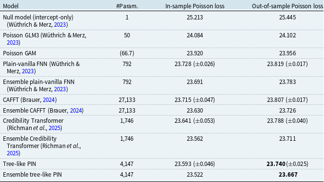
using the PD loss (3.1) as the objective function. Because early stopped stochastic gradient descent (SGD) training involves several elements of randomness, the presented results are averages over 10 SGD runs using different seeds (starting points) for the SGD algorithm, see also Wüthrich et al. (Reference Wüthrich, Richman, Avanzi, Lindholm, Maggi, Mayer, Schelldorfer and Scognamiglio2025, Section 5.3.8). That is, the loss figures are averages over 10 different fits (and in brackets we provide the observed standard deviations across these 10 runs). Moreover, we ensemble the predictors (by averaging over the predictors). This ensembling typically improves the predictive model, which is also verified in our PIN architecture, all these results are presented in Table 2.
Number of parameters, in-sample and out-of-sample Poisson deviance losses (units are in
 $10^{-2}$
); benchmark models are taken from Wüthrich and Merz (Reference Wüthrich and Merz2023, Table 7.9), Brauer (Reference Brauer2024, Tables 2 and 4) and Richman et al. (Reference Richman, Scognamiglio and Wüthrich2025, Table 2); for the ensemble models we state the number of parameters of a single model because each one is trained individually. The best out-of-sample performance is highlighted in bold

Table 2. Long description
The table presents a comparison of different models based on the number of parameters and their in-sample and out-of-sample Poisson deviance losses. The table has 10 rows and 4 columns. The columns are labeled ‘Model’, ‘#Param.’, ‘In-sample Poisson loss’, and ‘Out-of-sample Poisson loss’. The rows list various models along with their respective number of parameters and Poisson deviance losses. Row 1: Null model (intercept-only) (Wthrich & Merz, 2023), 1, 25.213, 25.445. Row 2: Poisson GLM3 (Wthrich & Merz, 2023), 50, 24.084, 24.102. Row 3: Poisson GAM, 66.7, 23.920, 23.956. Row 4: Plain-vanilla FNN (Wthrich & Merz, 2023), 792, 23.728 (0.026), 23.819 (0.017). Row 5: Ensemble plain-vanilla FNN (Wthrich & Merz, 2023), 792, 23.691, 23.783. Row 6: CAFFT (Brauer, 2024), 27,133, 23.715 (0.047), 23.807 (0.017). Row 7: Ensemble CAFFT (Brauer, 2024), 27,133, 23.630, 23.726. Row 8: Credibility Transformer (Richman et al., 2025), 1,746, 23.641 (0.053), 23.788 (0.040). Row 9: Ensemble Credibility Transformer (Richman et al., 2025), 1,746, 23.562, 23.711. Row 10: Tree-like PIN, 4,147, 23.593 (0.046), 23.740 (0.025). Row 11: Ensemble tree-like PIN, 4,147, 23.522, 23.667.
Let us discuss the results of Table 2. The benchmark models are taken from Wüthrich and Merz (Reference Wüthrich and Merz2023, Table 7.9), Brauer (Reference Brauer2024, Tables 2 and 4) and Richman et al. (Reference Richman, Scognamiglio and Wüthrich2025, Table 2). The null model does not consider any features, but it is just based on the empirical mean. Poisson GLM3 is a feature-engineered GLM having 50 parameters; this model is linear on the canonical scale and does not consider any interaction terms. The linearity of the GLM is challenged by the GAM using natural cubic splines. The complexity of this GAM cannot be expressed in terms of the number of parameters involved, but the GAM routine in Rdetermines the effective degrees of freedom (edf) using generalized cross-validation. The resulting edf in our example are 66.7, which means that suitably chosen natural cubic splines should be able to accommodate with roughly 67 parameters. These three fitted models have been fitted by minimizing the PD loss which is equivalent to perform MLE in the corresponding Poisson claims count model. We conclude that the GAM has the best out-of-sample performance among these three classical actuarial models, resulting in an out-of-sample loss of
 $23.956 \times 10^{-2}$
. This is the best benchmark that we can get if we do not consider any interaction terms between the feature components.
If we take a deep (plain-vanilla) FNN architecture of depth 3 with
 $(20,15,10)$
units and with two-dimensional embedding layers for the two categorical covariates, we receive a network architecture with 792 network parameters. If we fit this architecture with an early stopped SGD with 10 initializations, we receive an average out-of-sample loss of
 $23.819 \times 10^{-2}$
, and ensembling these 10 networks gives an out-of-sample performance of
 $23.783 \times 10^{-2}$
, thus, interaction modeling can clearly improve the GAM.
This deep plain-vanilla FNN architecture has been improved by using different versions of the transformer architecture of Vaswani et al. (Reference Vaswani, Shazeer, Parmar, Uszkoreit, Jones, Gomez, Kaiser and Polosukhin2017) modified to tabular input data. The powerful adoptions of Brauer (Reference Brauer2024, Table 4) and Richman et al. (Reference Richman, Scognamiglio and Wüthrich2025, Table 2) provide out-of-sample losses of
 $23.726 \times 10^{-2}$
and
 $23.711 \times 10^{-2}$
, respectively, for the ensemble versions. From Table 2, we conclude that our tree-like PIN proposal outperforms all these other methods. Thus, this data example verifies the superior predictive performance of the tree-like PIN over some of the most recent proposals in the literature. On top, as will be illustrated in the remainder of this article, it also gives us an intrinsic explainability, in contrast to most other network architectures.
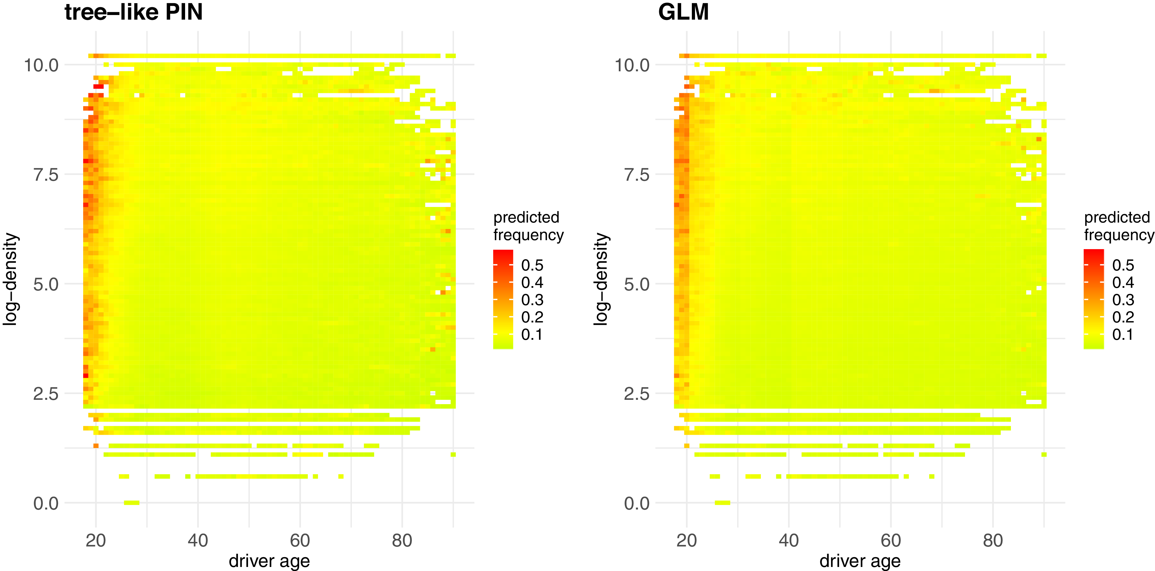
Heatmaps of predicted frequencies of (lhs) tree-like PIN and (rhs) GLM on all available features.

Figure 6 shows the resulting heatmaps of the predicted frequencies, with driver’s age on the
 $x$
-axis and log-density on the
 $y$
-axis; this is a two-dimensional marginal plot (M plot); see Apley and Zhu (Reference Apley and Zhu2020) and Wüthrich et al. (Reference Wüthrich, Richman, Avanzi, Lindholm, Maggi, Mayer, Schelldorfer and Scognamiglio2025, Section 9.3.4). Remark that we do not expect a smooth graph because the predicted frequencies were computed on nine feature components, and the graphs show a projected version to two of them (M plot), i.e., these are marginalized plots. For example, for high driver’s age, we see some sprinkling of red dots that can only be explained by analyzing the other features, e.g., it may be severely impacted by a high bonus-malus level; remark also that the portfolio is comparably sparse for large driver’s age values, that is why extreme expected frequency values do not average out.
4. Model explainability
4.1 PIN interaction importance
A notoriously difficult problem in machine learning models is explainability. Scholars have developed various post hoc measures of variable importance, e.g., permutation variable importance by Breiman (Reference Breiman2001) and Fisher et al. (Reference Fisher, Rudin and Dominici2018), or SHAP importance of Lundberg and Lee (Reference Lundberg and Lee2017) and Mayer and Stando (Reference Mayer and Stando2025) are two popular examples. When it comes to interactions, things become even more difficult. There is Friedman and Popescu (Reference Friedman and Popescu2008)’s
 $H^2$
-statistics which is a post hoc explainability tool that measures the impact of bivariate components on the regression function (by partial dependence functions). Apart from that, there is little guidance on how to measure the interaction strengths at a reasonable computational effort, i.e., testing pairwise interactions can be very costly.
Coming back to the PIN (2.9), we modify this function in a way so that we do not aim at getting the maximal predictive power, but we try to evaluate which shared interaction unit
 $h_{j,k}(\boldsymbol{x})$
contributes most to a loss decrease. For this, we consider the multi-output mapping
 \begin{equation} \boldsymbol{x} \,\mapsto \, ( f_{\mathrm {PIN},j,k} )_{1\le j \lt k \le q} \in \, {\mathbb R}^{q(q-1)/2}, \end{equation}
where for
 $1\le j\lt k \le q$
we set
 \begin{equation*} f_{\mathrm {PIN},j,k} = g\left (b+\sum _{l=1}^q w_{l,l} \, h_{l,l}(\boldsymbol{x})+ b_{j,k}+ w_{j,k} \, h_{j,k}(\boldsymbol{x})\right )\!, \end{equation*}
for biases
 $b_{j,k}\in {\mathbb R}$
and the remaining terms have the same structure as in (2.9). The first part of this multi-output regression function captures the main effects of the covariate components, this corresponds to the diagonal of the tensor (2.7). That is, the main effects are given by
 \begin{equation} b+\sum _{l=1}^q f_l(X_l) =b+\sum _{l=1}^q w_{l,l} \, h_{l,l}(\boldsymbol{x}), \end{equation}
where we make the link to the GAM (2.10). The remaining terms
 $h_{j,k}(\boldsymbol{x})$
in (4.1),
 $j\lt k$
, correspond to the off-diagonal terms of the pairwise interaction layer (2.7). Each component in (4.1) adds another interaction term to the diagonal (non-interacting) terms (4.2), and we can determine the term
 $h_{j,k}(\boldsymbol{x})$
,
 $j\lt k$
, that leads to the biggest decrease in out-of-sample loss when added to (4.2). The great thing is that we can fit all
 $q(q-1)/2$
interaction terms in the same gradient descent run, i.e., we apply the objective function for model fitting (simultaneously) to all components of (4.1), and jointly fit all components by just aggregating these component-wise losses
 \begin{eqnarray*} L_{\mathrm {AGGR}}(\mathcal{L}, (f_{\mathrm {PIN},j,k})_{j\lt k}) &=&\frac {1}{q(q-1)/2}\sum _{1\le j \lt k \le q} L_{\mathrm {PD}}(\mathcal{L}, f_{\mathrm {PIN},j,k}), \end{eqnarray*}
the latter is the average PD loss (3.1). This is possible here because we have isolated all interaction pairs in the pairwise interaction layer (2.7).
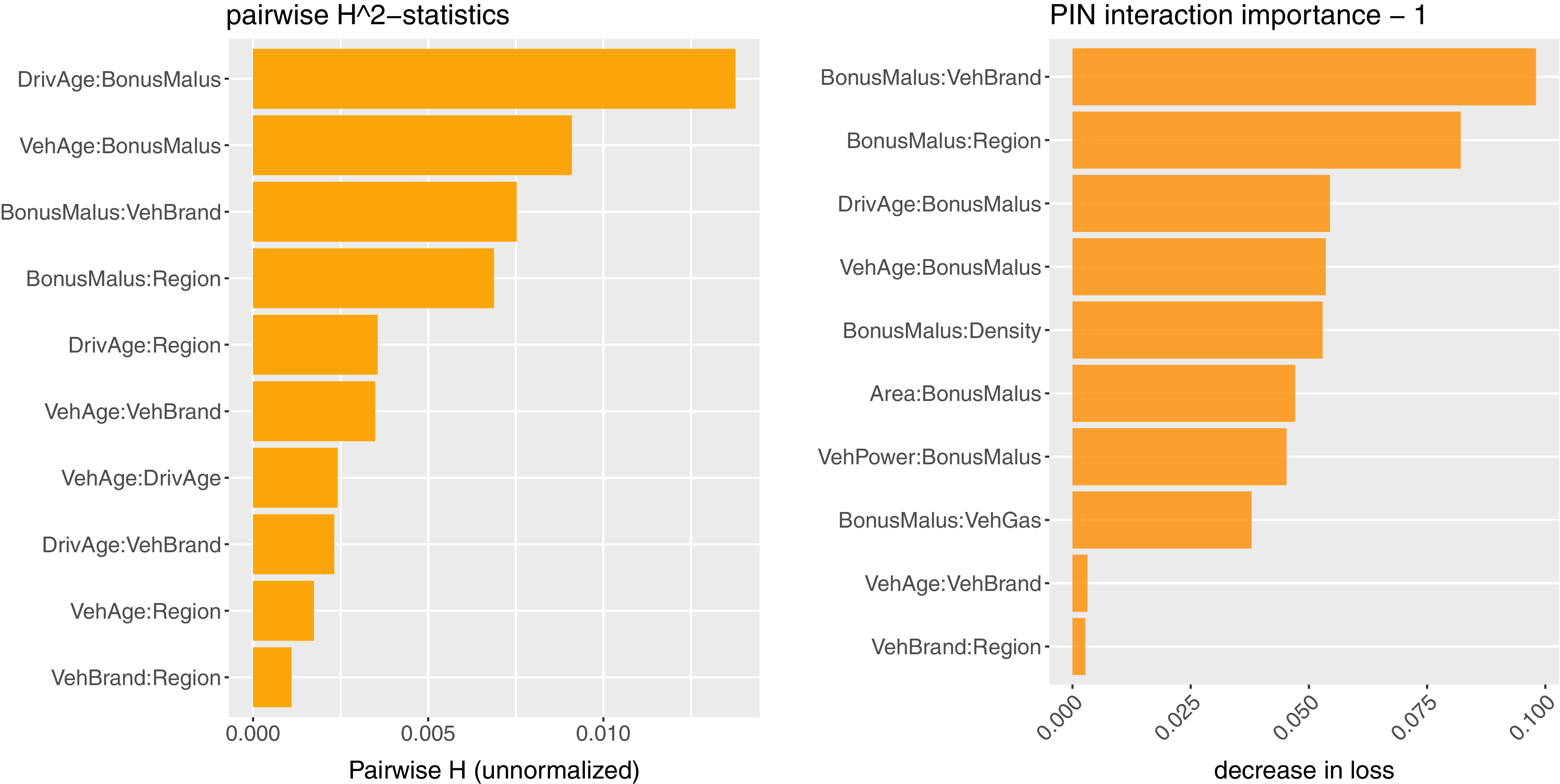
(lhs) Friedman and Popescu (Reference Friedman and Popescu2008)’s
 $H^2$
-statistics, and (rhs) PIN interaction importance.

In our example, we consider one further simplification, namely, we replace the diagonal (non-interacting) terms (4.2) by the fitted GAM terms that are considered to be optimal under the exclusion of interactions, see Table 2. This fitted GAM is kept fixed (frozen) and only the off-diagonal interaction terms in (4.1) are trained with SGD. The training of this multi-output PIN takes approximately 15 minutes on an ordinary laptop.Footnote 2 We then compute the decrease in out-of-sample loss compared to the GAM for each individual interaction term,
 $j\lt k$
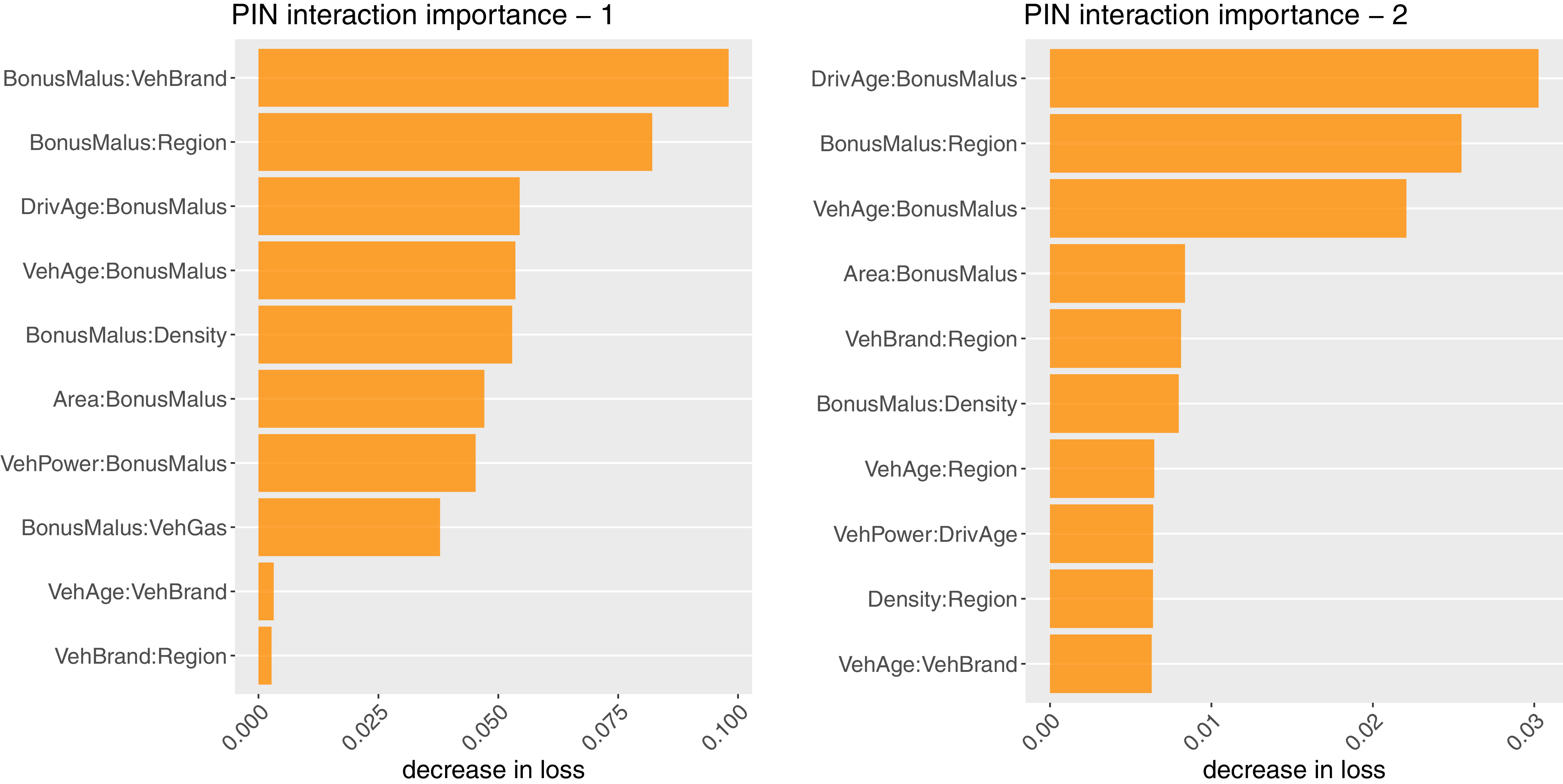
. Figure 7 (rhs) shows the results (ranked by size). The biggest decrease in loss compared to the GAM can be achieved by adding an interaction term for (BonusMalus:VehBrand), and the second biggest decrease is obtained by adding (BonusMalus:Region).
Figure 7 (lhs) illustrates the Friedman and Popescu (Reference Friedman and Popescu2008)
 $H^2$
-statistics computed for the full PIN model. In our experiments, this procedure requires around 90 minutes (typically one chooses a small background dataset to speed up computations). Not surprisingly, the same feature interactions seem to be the most impactful ones, but the order of the most important interactions is different. Friedman–Popescu’s
 $H^2$
-statistics studies the partial dependence function in a fully fitted model (which can be seen as a top-down view – backward selection), whereas our PIN approach considers which interaction should be added to have the biggest impact on the prediction accuracy (which is more of a bottom-up consideration – forward selection). Thus, we can interpret this as a forward selection of interaction terms, similar to the forward selection model building in GLMs. Moreover, Friedman–Popescu’s
 $H^2$
-statistics is based on partial dependence plots (PDPs), which have the weakness that they are not necessarily reliable in cases where the feature components are highly correlated, because PDPs extrapolate the regression function to rare or impossible covariate combinations (e.g., car drivers aged 20 with 10 years of driving experience), where the regression function is typically poorly estimated or undefined, respectively. Not surprisingly, this weakness also translates to the
 $H^2$
-statistics. Our method does not suffer from this weakness, since the contribution of each pairwise interaction is evaluated on the empirically observed portfolio – on the empirical population distribution – and assessing each interaction independently of all others. As a consequence, the importance measure of each pairwise interaction remains meaningful even in the presence of feature correlations. Naturally, as is also common in the GLM forward selection process, if there are two highly correlated feature components that interact with a third component, after including the first strong interaction, the second one may no longer be needed. We discuss this next.
(lhs) PIN interaction importance – 1st round (this plot is identical to Figure 7, rhs), and (rhs) PIN interaction importance – 2nd round.

Similar to the method of forward selection in GLMs, we add the most significant interaction term (BonusMalus:VehBrand) to the diagonal regression model (4.2). We also freeze this interaction term, and we repeat the same fitting strategy to find the second most important interaction term, after (BonusMalus:VehBrand) has been added to the model. The result of this second round of forward selection is shown in Figure 8 (rhs), and it is compared to the first round results on the left-hand side. The second interaction that should be added is (DrivAge:BonusMalus). This gives a systematic way of model building that may also be useful in improving GLMs and GAMs; this is similar to the forward selection algorithm of GLM model building. Note that this forward selected model should be refitted simultaneously on all included terms, because in this forward inclusion process, we always freeze the previously selected terms, and an additional re-fitting (fine-tuning) step may find a more optimal jointly learned model on the selected pairwise interaction components.
4.2 SHapley’s Additive exPlanation
There is another very remarkable property of the tree-like PIN architecture, namely, it allows for a very efficient computation of SHapley’s Additive exPlanation (SHAP) as introduced by Lundberg and Lee (Reference Lundberg and Lee2017). Shapley values originate from cooperative game theory. They are used to share a total payoff of a cooperative game in a fair way among
 $q$
players; see Shapley (Reference Shapley1953). Denote by
 $\mathcal{C} \subseteq \mathcal{Q}=\{1,\ldots , q\}$
any coalition of
 $q$
players. Based on Shapley’s fairness axioms, there is precisely one way to allocate the total payoff to the
 $q$
players of the cooperative game, resulting in the Shapley values
 $\psi _j$
assigned to players
 $j \in \mathcal{Q}$
, given by
 \begin{equation} \psi _j = \frac {1}{q} \sum _{\mathcal{C} \subseteq \mathcal{Q} \setminus \{j\}} {\begin{pmatrix}q-1\\|\mathcal{C}|\end{pmatrix}}^{-1} (\nu (\mathcal{C} \cup \{j\}) - \nu (\mathcal{C}) ), \qquad \text{ for all }j \in {\mathcal{Q}}, \end{equation}
for a given value function
 $\mathcal{C}\mapsto \nu (\mathcal{C})$
. In fact, starting from the given value function
 $\nu$
, the Shapley values
 $(\psi _j)_{j=1}^q$
are the unique solution to a set of four axioms called Shapley’s fairness axioms; see Shapley (Reference Shapley1953) and Lundberg and Lee (Reference Lundberg and Lee2017).
There are two equivalent reformulations of the Shapley values (4.3), namely, there is the kernel SHAP formulation of Lundberg and Lee (Reference Lundberg and Lee2017, Theorem 2), and there is the permutation SHAP version of Štrumbelj and Kononenko (Reference Štrumbelj and Kononenko2010, Reference Štrumbelj and Kononenko2014). In this work, we focus on the permutation SHAP formulation. Denote by
 $\pi =(\pi _1,\ldots , \pi _q )$
a permutation of the ordered set
 $(1,\ldots , q)$
. Let
 $\kappa (j) \in \mathcal{Q}$
be the index defined by
 $\pi _{\kappa (j)}=j$
and set
 \begin{equation} \mathcal{C}_{\pi , j} = \{ \pi _1,\ldots , \pi _{\kappa (j)-1} \}\,\subset \,\mathcal{Q}. \end{equation}
These are all components of
 $\pi$
preceding
 $\pi _{\kappa (j)}=j$
; for
 $\kappa (j)=1$
, this is the empty set
 $\emptyset$
. The permutation SHAP version of Štrumbelj and Kononenko (Reference Štrumbelj and Kononenko2010, Reference Štrumbelj and Kononenko2014) proves that the Shapley values (4.3) can equivalently be computed by
 \begin{equation} \psi _j = \frac {1}{q!} \sum _{\pi }\nu (\mathcal{C}_{\pi , j}\cup \{j\} ) -\nu (\mathcal{C}_{\pi , j} ) , \end{equation}
where the summation runs over all permutations
 $\pi$
. These are
 $q!$
permutations
 $\pi$
, which can be an extremely large number making Shapley values computationally unattainable for large
 $q$
. However, there is a nice result which says that if the value function
 $\nu$
only includes interactions of maximal order two, then an arbitrary permutation
 $\pi =(\pi _1,\ldots , \pi _q)$
, and its reverted version
 $\rho (\pi )=(\pi _q,\ldots , \pi _1)$
is sufficient to compute the Shapley values
 \begin{equation} \psi _j = \frac {1}{2} (\nu (\mathcal{C}_{\pi , j}\cup \{j\} ) -\nu (\mathcal{C}_{\pi , j} ) +\nu (\mathcal{C}_{\rho (\pi ), j}\cup \{j\} ) -\nu (\mathcal{C}_{\rho (\pi ), j} ) ), \end{equation}
if the value function
 $\nu$
is a bilinear form; see Mayer and Wüthrich (Reference Mayer and Wüthrich2025, Proposition 3.1). For example, the permutation
 $\pi =(1,\ldots , q)$
and its reverted version
 $\rho (\pi )=(q,\ldots , 1)$
do the job.
For explaining machine learning predictions, one typically works on the link scale, i.e., one drops the link function
 $g$
in (2.9). For a given feature
 $\boldsymbol{x}$
, this motivates the total value of the grand coalition
 $\mathcal{Q}$
 \begin{equation*} \nu (\mathcal{Q}):=\nu _{\boldsymbol{x}}(\mathcal{Q}):= g^{-1} (f_{\mathrm {PIN}}(\boldsymbol{x}) )= \sum _{1\le j \le k \le q} w_{j,k} \, h_{j,k}(\boldsymbol{x})+b. \end{equation*}
This is the prediction made by
 $\boldsymbol{x}=(x_1,\ldots , x_q)^\top$
, and we want to explain how the feature components
 $x_j$
contribute to this prediction. This requires the choice of the value function
 $\nu (\mathcal{C})=\nu _{\boldsymbol{x}}(\mathcal{C})$
for any coalition
 $\mathcal{C}\subset \mathcal{Q}$
if the elements in
 $\mathcal{Q}\setminus \mathcal{C}$
are masked (not available for prediction). The most popular choice for describing the masking is the so-called interventional SHAP version, in our case given by
 \begin{equation} \nu (\mathcal{C}):=\nu _{\boldsymbol{x}}(\mathcal{C}) := {\mathbb E}\left [\sum _{1\le j \le k \le q} w_{j,k} \, h_{j,k} (\boldsymbol{x}_\mathcal{C}, \boldsymbol{X}_{\mathcal{Q}\setminus \mathcal{C}} )+b\right ], \end{equation}
where the components
 $\boldsymbol{x}_\mathcal{C}=(x_j)_{j \in \mathcal{C}}$
are kept fixed and the components
 $\boldsymbol{X}_{\mathcal{Q}\setminus \mathcal{C}}=(X_j)_{j \in \mathcal{Q}\setminus \mathcal{C}}$
are resampled from the population distribution
 $\boldsymbol{X} \sim {\mathbb P}$
. An important point in the subsequent computation of the Shapley values is that each term
 $h_{j,k}$
in (4.7) only depends on the components
 $(j,k)$
, i.e., we only have pairwise interactions, see (2.6). That is, by a slight abuse of notation,
 \begin{equation*} h_{j,k} (\boldsymbol{x}_\mathcal{C}, \boldsymbol{X}_{\mathcal{Q}\setminus \mathcal{C}} ) = \left \{ \begin{array}{ll} h_{j,k}(x_j, x_k) & \text{ if $j,k \in \mathcal{C}$,}\\[2pt] h_{j,k}(X_j, x_k) & \text{ if $j \in \mathcal{Q} \setminus \mathcal{C}$ and $k \in \mathcal{C}$,}\\[2pt] h_{j,k}(x_j, X_k) & \text{ if $j \in \mathcal{C}$ and $k\in \mathcal{Q} \setminus \mathcal{C}$,}\\[2pt] h_{j,k}(X_j, X_k) & \text{ if $j,k \in \mathcal{Q} \setminus \mathcal{C}$.}\\ \end{array} \right . \end{equation*}
This interventional SHAP formula (4.7) is usually estimated empirically. For this, we select a background set
 $\mathcal{B}$
from the learning sample
 $\mathcal{L}$
. This allows one to determine the value function empirically by
 \begin{equation} \widehat {\nu }(\mathcal{C})=\widehat {\nu }_{\boldsymbol{x}}(\mathcal{C}) = \frac {1}{|\mathcal{B}|}\sum _{i \in \mathcal{B}} \left [\sum _{1\le j \le k \le q} w_{j,k} \, h_{j,k}\left (\boldsymbol{x}_\mathcal{C}, \boldsymbol{X}^{(i)}_{\mathcal{Q}\setminus \mathcal{C}}\right )+b\right ], \end{equation}
where
 $\boldsymbol{X}^{(i)}$
is the
 $i$
-th instance of the background dataset.
The crucial point now is that the value function
 $\mathcal{C} \mapsto \widehat {\nu }(\mathcal{C})=\widehat {\nu }_{\boldsymbol{x}}(\mathcal{C})$
only involves interactions of maximal order two. Therefore, the paired permutation SHAP formula (4.6) applies (and it is exact for the selected value function
 $\widehat {\nu }=\widehat {\nu }_{\boldsymbol{x}}$
). This requires
 $2(q+1)$
evaluations of the value function
 $\widehat {\nu }$
, and each value function evaluation requires
 $|\mathcal{B}|$
computations of PIN predictions, see (4.8). Thus, altogether, the SHAP decomposition of the prediction
 $g^{-1}(f_{\mathrm {PIN}}(\boldsymbol{x}) )$
requires
 $2(q+1)|\mathcal{B}|$
PIN network computations for computing the exact Shapley values
 $(\psi _j)_{j=1}^q$
of the value function
 $\widehat {\nu }$
. Any other network architecture that involves higher-order interactions would need
 $q!\, |\mathcal{B}|$
network computations for receiving the exact Shapley values of the corresponding estimated interventional SHAP value function; thus, the order of computations grows as
 $q!$
instead of
 $2(q+1)$
as in our tree-like PIN case.
We revisit the PIN architecture depicted in Table 1 having the best predictive performance of all models presented in Table 2. We emphasize that this network architecture only considers interactions of order two on the link scale; thus, the paired-sampling permutation SHAP formula (4.6) applies, and it gives exact results, for instance, we can use the permutation pair
 $\pi =(1,\ldots , q)$
and
 $\rho (\pi )=(q,\ldots , 1)$
. As background dataset, we select at random
 $|\mathcal{B}|=2,000$
instances from the learning set. This allows us to decompose the predictions
 $g^{-1}(f_{\mathrm {PIN}}(\boldsymbol{x}) )$
of selected instances
 $\boldsymbol{x}$
. Decomposing 100 predictions takes 23 s on an ordinary laptop (see footnote on page 36).
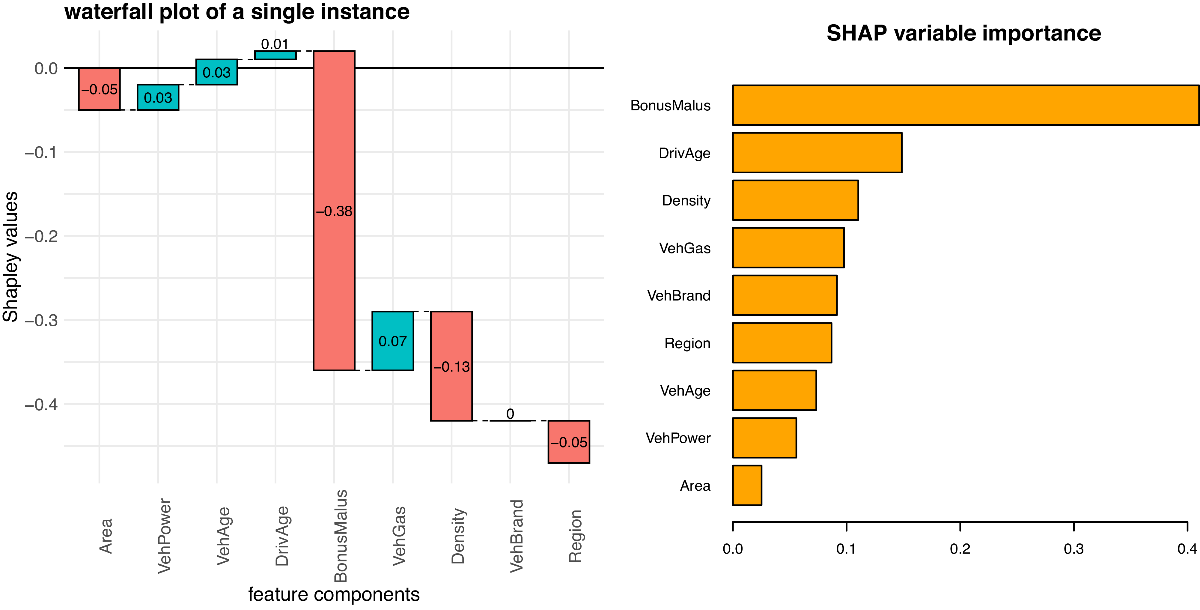
(lhs) SHAP waterfall graph
 $(\psi _j)_{j=1}^q$
of a single instance
 $\boldsymbol{x}$
and (rhs) SHAP variable importance.

The left-hand side of Figure 9 shows the Shapley values
 $(\psi _j)_{j=1}^q$
of a single instance
 $\boldsymbol{x}$
. We have global mean of the background dataset of
 $\widehat {\nu }_{\boldsymbol{x}}(\emptyset )=-2,776$
, and the prediction of feature
 $\boldsymbol{x}$
is given by
 $\widehat {\nu }_{\boldsymbol{x}}(\mathcal{Q})=g^{-1}(f_{\mathrm {PIN}}(\boldsymbol{x}) )=-3.239$
. Thus, feature
 $\boldsymbol{x}$
has a prediction being
 $-0.463$
below average. The Shapley values
 $(\psi _j)_{j=1}^q$
illustrated in Figure 9 (lhs) show how this lower prediction can be explained. The biggest decrease is explained by the bonus-malus level and the density features, whereas the vehicle gas feature leads to the biggest increase in the explanation of this difference from
 $\widehat {\nu }_{\boldsymbol{x}}(\emptyset )$
to
 $\widehat {\nu }_{\boldsymbol{x}}(\mathcal{Q})$
.
Going from local to global SHAP explanations, we can decompose the predictions
 $g^{-1}(f_{\mathrm {PIN}}(\boldsymbol{x}_i))$
of many instances
 $(\boldsymbol{x}_i)_{i \in \mathcal{I}}$
, for a randomly selected subset
 $\mathcal{I}$
of the entire data. This provides us with SHAP decompositions
 $(\psi ^{(i)}_j)_{j=1}^q$
, which allow us to consider different statistics. The following analysis is based on
 $|\mathcal{I}|=1,000$
instances
 $\boldsymbol{x}_i$
that have been decomposed by the paired-sampling permutation SHAP method. SHAP variable importance is then obtained by considering
 \begin{equation*} \overline {\psi }_j = \frac {1}{|\mathcal{I}|} \sum _{i \in \mathcal{I}} |\psi ^{(i)}_j|. \end{equation*}
Figure 9 (rhs) shows these importance measures
 $\overline {\psi }_j$
for all feature components
 $j \in \mathcal{Q}$
. The most significant role is played by the bonus-malus level (past claims history) followed by the driver’s age variable and at the other end is the area code that seems to be the least important variable.
(lhs) Dependence between driver’s age and the bonus-malus variable, this graph is taken from Wüthrich and Merz (Reference Wüthrich and Merz2023, Figure 13.12), and (rhs) Shapley values
 $\psi _j^{(i)}$
of the selected 100 instances
 $i\in \mathcal{I}$
for the covariate
 $j=\texttt {DrivAge}$
; the coloring is the bonus-malus level of these instances.

Figure 10 Long description
Panel A: A box plot shows the relationship between driver age (DrivAge) and bonus-malus levels (BonusMalus). The x-axis represents driver age in years, grouped into categories, while the y-axis represents the bonus-malus levels ranging from 50 to 120. The box plot displays the distribution of bonus-malus levels for each age group, with visible trends showing higher bonus-malus levels for younger drivers and a decrease in levels as driver age increases. Panel B: A scatter plot illustrates the Shapley values for the covariate driver age (DrivAge) against the driver age. The x-axis represents driver age in years, and the y-axis represents Shapley values ranging from -0.4 to 0.2. The points are colored according to the bonus-malus levels, with a color gradient from red to green indicating lower to higher bonus-malus levels. The plot shows a pattern where Shapley values vary with driver age, with notable clustering and trends visible across different age groups.
In Figure 10 (rhs), we analyze the 1,000 decomposed instances
 $\boldsymbol{x}_i$
,
 $i\in \mathcal{I}$
. The plot shows the Shapley values
 $\psi ^{(i)}_j$
of these 1,000 instances for the variable
 $j =\texttt {DrivAge}$
. This driver age variable has its strongest interaction with the bonus-malus level, see Figure 8, and the coloring of the Shapley values in Figure 10 (rhs) is selected according to these bonus-malus levels. We observe that the driver’s age variable has a decreasing effect on the prediction for drivers’ ages below 40 (negative Shapley values) and an increasing effect for ages between 40 and 60 (positive Shapley values). To fully understand this picture, one needs to understand the interaction with the bonus-malus level, and we observe for drivers’ ages below 40, that this positive age effect especially holds for low bonus-malus levels. In fact, there is a strong dependence between the driver’s age variable and the bonus-malus level for drivers’ ages below 40, see boxplot of Figure 10 (lhs), because new drivers start at a bonus-malus level of 100 (yellow color in Figure 10, rhs). This level decreases in every year that the driver is free of accidents, and otherwise it increases. Therefore, young drivers typically have a higher bonus-malus level than mature drivers (in a low-frequency environment), and the Shapley values in Figure 10 (rhs) tell us that young drivers with a lower bonus-malus level (green colors) get a decrease compared to their older peers in the same bonus-malus class. Of course, this interaction makes perfect sense. This completes the French MTPL example.
5. A second real-world data example
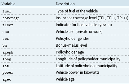
To further assess the performance of the proposed tree-like PIN architecture, we consider a second dataset. We select the Belgian MTPL dataset available from Dutang et al. (Reference Dutang, Charpentier and Gallic2024), comprising 163,212 individual insurance policies. Also in this case, the aim consists of forecasting claims frequencies conditional on a set of observed risk characteristics. The dataset contains 11 features, and these are detailed in Table 3.
Policy-level covariates and their descriptions

Table 3. Long description
The table has 11 rows and 2 columns. The columns are labeled ‘Variable’ and ‘Description’. Row 1: Variable, fuel; Description, Type of fuel of the vehicle. Row 2: Variable, coverage; Description, Insurance coverage level (TPL, TPL+, TPL++). Row 3: Variable, fleet; Description, Indicator for fleet vehicle (yes/no). Row 4: Variable, use; Description, Vehicle use (private or work). Row 5: Variable, sex; Description, Policyholder gender. Row 6: Variable, bm; Description, Bonusmalus level. Row 7: Variable, ageph; Description, Policyholder age. Row 8: Variable, long; Description, Longitude of policyholder municipality. Row 9: Variable, lat; Description, Latitude of policyholder municipality. Row 10: Variable, power; Description, Vehicle power in kilowatts. Row 11: Variable, agec; Description, Vehicle age.
We adopt the same splitting scheme as before, using a 90–10% learning-test split, and we standardize all continuous input features. The same PIN architecture used for the French dataset is employed. The 10 continuous and binary input variables are processed through a separate embedding network, see (2.2), with layer sizes
 $d' = 20$
and
 $d = 10$
. The single categorical variable (coverage) is processed via an entity embedding, see (2.1), with dimension
 $d = 10$
. The application of this tokenization procedure yields a tensor representation
 $\boldsymbol{\phi } = \boldsymbol{\phi }(\boldsymbol{x}) \in \mathbb{R}^{10 \times 11}$
, from which pairwise interaction terms are constructed. In total, this results in
 $10 \times 11/2 = 66$
interaction tokens
 $\boldsymbol{e}_{j,k} \in \mathbb{R}^{10}$
, for
 $1 \le j \lt k \le 11$
. Also in this case, the shared interaction network defined in (2.5) is selected as a two-layer architecture with hidden layer dimensions
 $d_1 = 30$
and
 $d_2 = 20$
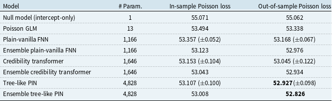
. The comparison is conducted in terms of number of parameters, in-sample and out-of-sample PD losses w.r.t. a selection of benchmark models: Poisson null, Poisson GLM, plain vanilla FNN, and the credibility transformer. For the neural network-based models, performance is evaluated both in terms of average results over 10 SGD runs and ensemble predictions. Table 4 gives the results.
Number of parameters, in-sample and out-of-sample Poisson deviance losses (units are in
 $10^{-2}$
) on the Belgian MTPL dataset; for the ensemble models, we state the number of parameters of a single model because each one is trained individually. The best out-of-sample performance is highlighted in bold

Table 4. Long description
A table with two columns: Variable and Description. The table lists 12 variables along with their descriptions. Row 1: Variable: fuel, Description: Type of fuel of the vehicle. Row 2: Variable: coverage, Description: Insurance coverage level (TPL, TPL+, TPL++). Row 3: Variable: fleet, Description: Indicator for fleet vehicle (yes/no). Row 4: Variable: use, Description: Vehicle use (private or work). Row 5: Variable: sex, Description: Policyholder gender. Row 6: Variable: bm, Description: Bonus-malus level. Row 7: Variable: ageph, Description: Policyholder age. Row 8: Variable: long, Description: Longitude of policyholder municipality. Row 9: Variable: lat, Description: Latitude of policyholder municipality. Row 10: Variable: power, Description: Vehicle power in kilowatts. Row 11: Variable: agec, Description: Vehicle age.
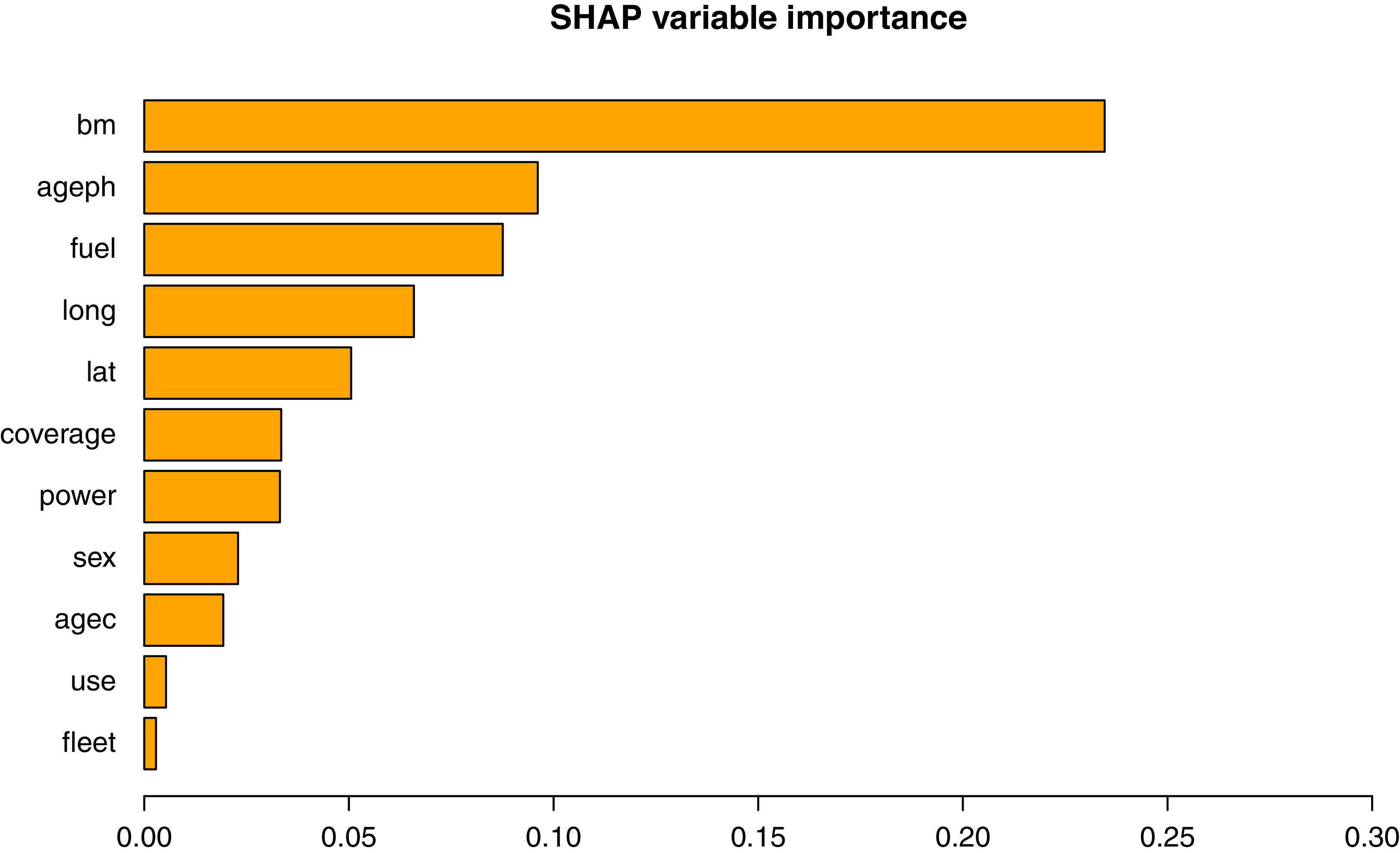
SHAP variable importance on Belgian MTPL dataset.

The tree-like PIN achieves the best out-of-sample predictive performance also on this second dataset, outperforming all other considered benchmark models in terms of PD loss. Moreover, the ensemble version of the tree-like PIN further enhances the predictive accuracy, which appears superior w.r.t. the plain-vanilla FNN and the credibility transformer.
Next, we perform an explainability analysis to identify the features and pairwise feature interactions that most strongly impact the model’s predictions. We begin by discussing the SHAP variable importance results. Figure 11 reports a bar plot of SHAP feature importance, showing that the model is mainly driven by the bonus-malus variable (bm), similarly to what is observed on the French dataset. The next most influential predictors are ageph and fuel. Geographic coordinates (long and lat) and coverage produce an intermediate contribution.
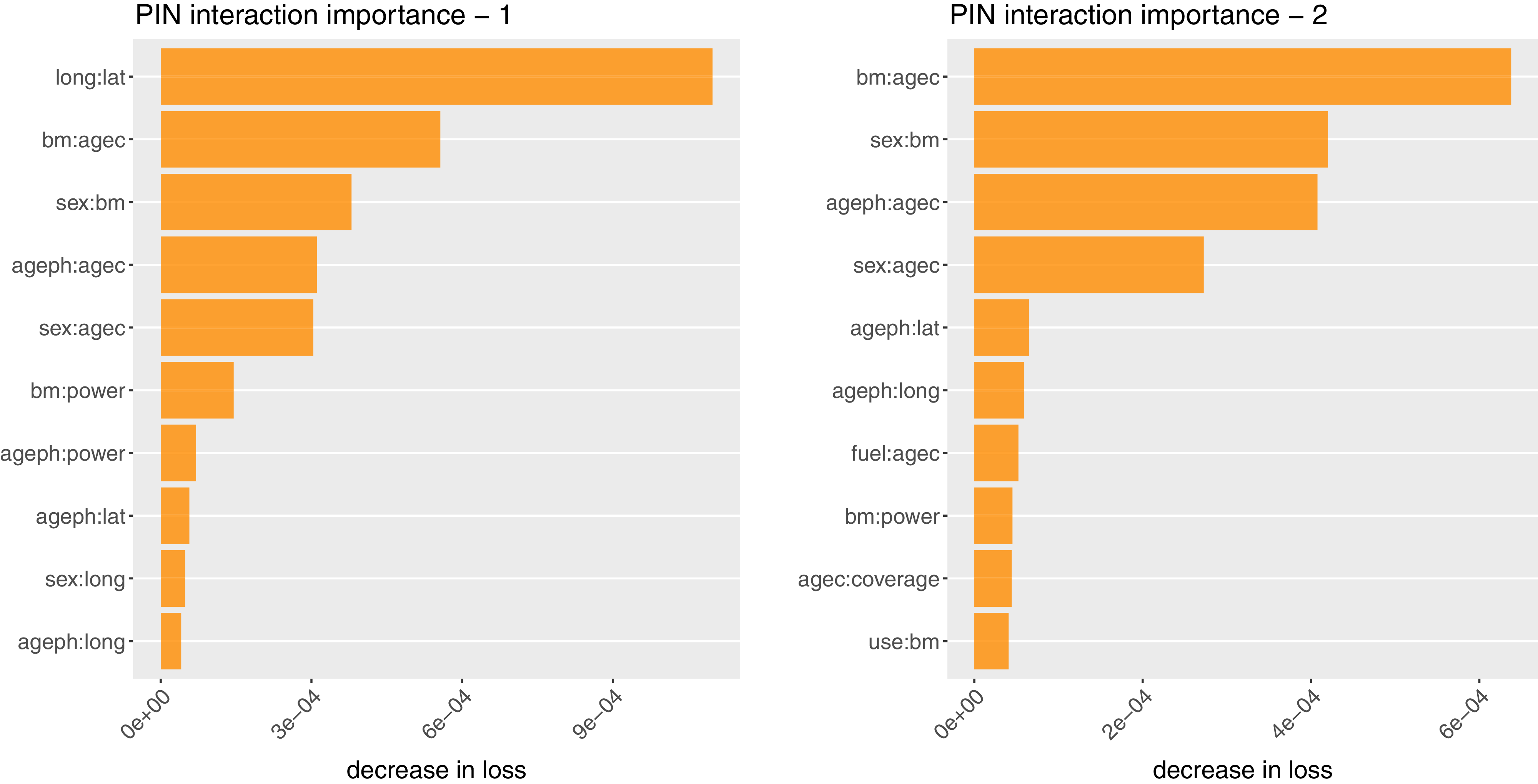
Beyond the individual contribution of each covariate, we also investigate the most relevant interactions among covariates. Following the procedure described above, we train the multi-output PIN model defined in (4.1). The objective is to identify the pairwise interactions that lead to the largest reductions in the loss function and, consequently, provide the strongest contribution to the predictive performance. Figure 12 summarizes the outcomes of the two-step selection procedure. The left panel reports the ranking obtained in the first round, where the interaction-free GAM model is frozen and all pairwise interactions are evaluated. The right panel shows the ranking from the second round, where the interaction selected at the first step is frozen as well. In the first round (lhs), the strongest interaction involves the geographical coordinates (long and lat). This highlights that, although their marginal effects are not among the most significant ones, their interaction, which captures more informative spatial patterns, has the most significant impact. In the second round, once the main spatial interaction has been fixed, the most important interaction emerges between the bonus-malus indicator and the age of the vehicle. Interestingly, this result is consistent with what we previously observed for the French MTPL dataset, where the same combination appeared among the most influential interaction effects.
(lhs) PIN interaction importance on Belgian MTPL dataset – 1st round, and (rhs) PIN interaction importance – 2nd round.

6. Conclusion
This paper introduces the tree-like PIN, a novel neural network architecture designed to explicitly capture pairwise covariate interactions in tabular data. Modeling such interactions is essential in predictive tasks, as they reveal how covariates jointly affect the response beyond their individual contributions. The tree-like PIN embeds each input covariate into a latent space, and it models pairwise interactions through a shared FNN equipped with a centered hard sigmoid activation, which replicates the partitioning behavior of decision trees. The use of a shared network ensures parameter efficiency, while the inclusion of interaction-specific learnable parameters preserves the flexibility required to capture heterogeneous dependencies across covariate pairs.
Numerical analysis is performed on two commonly used real-world insurance datasets. The results show that the tree-like PIN achieves a strong predictive performance, and it consistently outperforms both traditional benchmarks and recently introduced neural network architectures, including the credibility transformer of Richman et al. (Reference Richman, Scognamiglio and Wüthrich2025). In addition, the tree-like PIN enhances model interpretability by enabling the analysis of how pairs of covariates jointly contribute to the response. Since this architecture only involves pairwise interactions, it allows for a very efficient way of computing SHAP by the paired-sampling permutation SHAP method. The paper also highlights connections between the functioning of the tree-like PIN architecture and existing methods. Despite its novel architecture, the tree-like PIN shares similarities with GA
 $^{2}$
Ms, gradient boosting, and GNNs.
Possible future research directions include the incorporation of regularization techniques to promote sparsity, thereby enabling an automated selection of the most relevant interaction pairs and improving model generalization. Such regularization strategies could also be employed to penalize terms involving protected attributes, supporting the development of fairer predictive models. Another promising avenue is the extension of the tree-like PIN architecture to time-series data, enabling the joint modeling of temporal dependencies and feature interactions.
Acknowledgements
The authors thank the two anonymous referees whose comments helped to significantly improve the manuscript.
Code and data availability statement
Code and data are available from the GitHub repository: https://github.com/wueth/Tree-Like-PIN.
Competing interests
The authors are not aware of any conflict of interest.

 σhard(xj+xk)
 σhard(xj/3+xk)
 j
 d=1
 d=4
 10−2
 H2
 (ψj)j=1q
 x

 ψj(i)
 i∈I
 j=DrivAge
 10−2

 Open access

