





1. Introduction
Sufficient energy confinement is essential to sustain burning plasma conditions in reactor-scale tokamaks such as ITER (Joffrin Reference Joffrin2024; Yoshida Reference Yoshida2025). Operation in the high-confinement (H-mode) regime is inevitably accompanied by edge-localised modes (ELMs), which expel bursts of particles and energy from the pedestal, imposing transient heat loads on plasma-facing components and challenging long-pulse operation (Xie et al. Reference Xie2023; Paschalidis et al. Reference Papadopoulos, Glytsis, Ram and Hizanidis2024; Wu et al. Reference Wu2024). Understanding and controlling ELMs thus remains a central task in magnetic confinement fusion research.
The ELMs feature filamentary structures with densities comparable to the pedestal top. Thomson scattering experiments on MAST and DIII-D have measured their high densities (Kirk Reference Kirk2004; Kirk et al. Reference Kirk, Koch, Scannell, Wilson, Counsell, Dowling, Herrmann, Martin and Walsh2006; Eldon Reference Eldon2012), while reflectometry measurements on Globus-M2 and KSTAR indicate that these filaments can strongly perturb microwave signals (Seo Reference Seo2022; Yashin Reference Yashin2023). In particular, frequency-modulated continuous-wave (FMCW) reflectometry, with its high temporal resolution (Kim et al. Reference Kim, Doyle, Rhodes, Peebles, Rettig and Luhmann1997; Conway et al. Reference Conway, Vayakis, Fessey and Bartlett1999; Muscatello et al. Reference Muscatello2020; Silva et al. Reference Silva, Dias, Santos, da Silva and Gonçalves2021; Morales Reference Morales2024), reveals frequency hopping in the intermediate-frequency (IF) spectrum during ELM events (Conway et al. Reference Conway, Vayakis, Fessey and Bartlett1999; Kirk et al. Reference Kirk, Koch, Scannell, Wilson, Counsell, Dowling, Herrmann, Martin and Walsh2006; Seo Reference Seo2022; Maylis Reference Maylis2025), highlighting its potential to probe both density profiles and the filament dynamics.
Previous full-wave and numerical studies have also examined the influence of filaments or edge density structures on microwave and radio-frequency (RF) wave propagation. Vicente et al. investigated fixed-frequency O-mode reflectometry of plasma filaments using a two-dimensional finite-difference time-domain full-wave model (Vicente et al. Reference Vicente, da Silva, Heuraux, Manso, Conway and Silva2014). Yashin et al. modelled filament-induced backscattering in Doppler backscattering diagnostics (Yashin et al. Reference Yashin, Teplova, Zadvitskiy and Ponomarenko2022). More broadly, Biswas et al. developed a hybrid full-wave/Markov-chain model for RF scattering from scrape-off-layer filaments (Biswas et al. Reference Biswas, Shiraiwa, Baek, Bonoli, Ram and White2021), and Papadopoulos et al. studied full-wave scattering by randomly modulated density interfaces in edge plasmas (Papadopoulos et al. Reference Papadopoulos, Glytsis, Ram and Hizanidis2021). These studies collectively show that filamentary or interface-like edge structures can substantially modify wave propagation and spectral response. Unlike these studies, which mainly addressed fixed-frequency reflectometry, Doppler backscattering or more general RF scattering by edge structures, the present work focuses on FMCW reflectometry and on how filament-induced changes in cutoff topology give rise to IF frequency hopping and multiple effective return paths, with qualitative comparison with EAST observations.
Despite these observations, most measurements remain qualitative. Direct information on filament parameters such as radial width and peak density requires complementary diagnostics, leaving the interpretation of reflectometry signals in terms of the filament dynamics incomplete and their parameter dependence unclarified.
In this work, we employ two-dimensional full-wave simulations based on the finite-difference time-domain method (Yee Reference Yee1966; Wang Reference Wang2017; da Silva Reference da Silva2022; Tsironis & Papadopoulos Reference Tsironis and Papadopoulos2023; da Silva Reference da Silva2024) to investigate the basic mechanisms by which localised ELM filaments modify FMCW reflectometry signals. Rather than attempting a discharge-specific synthetic diagnostic for EAST, we adopt a simplified slab model that allows controlled scans of filament peak density, radial width and beam-axis displacement, and thereby isolates their respective impacts on the reflectometry response. Comparison with EAST observations is therefore intended at a qualitative level, focusing on robust signal morphology such as abrupt IF frequency hopping rather than on discharge-specific quantitative agreement. A fully quantitative EAST-specific validation would require independent measurements of the instantaneous filament width, density amplitude, radial location and two- or three-dimensional morphology near the reflectometer cutoff layer.
2. Simulation and model
2.1. Background density and filaments
We consider a simplified two-dimensional slab geometry in the radial–poloidal plane (x, y) to investigate the basic mechanisms by which localised edge filaments perturb FMCW reflectometry. The purpose of the present model is not to reproduce a specific EAST discharge quantitatively, but to isolate the first-order roles of filament peak density, radial width and beam-axis displacement in a controlled and computationally tractable setting. Compared with a device-specific model in the real EAST geometry, such a reduced description avoids additional complexity associated with toroidal magnetic geometry, diagnostic port geometry, antenna pattern and discharge-dependent equilibrium reconstruction, thereby making the physical origin of the signal modifications more transparent.
We therefore adopt an idealised equilibrium profile with a relatively weak density gradient. This choice is made to facilitate controlled parameter scans and to keep the numerical resolution requirement tractable, while still maintaining adequate resolution of the equilibrium density gradient on the grid. In the present model, the equilibrium density varies only along the radial direction, and the corresponding density-gradient scale length
 $L_{n}$
remains well resolved on the grid (
 $L_{n}\gg \Delta x$
) (Igami Reference Igami2016; da Silva Reference da Silva2022). The model should therefore be regarded as a first-step, physics-oriented description for mechanism identification rather than a discharge-specific predictive model, while more realistic EAST-specific synthetic diagnostics are left for future work.
A uniform toroidal magnetic field B is assumed. For O-mode propagation, the refractive index is independent of B, so the cold-plasma permittivity can be treated as a scalar. The corresponding O-mode dispersion relation is
 \begin{align}N^{2}(x,y,\omega )=1-\frac{{\omega }_{pe}^{2}}{\omega ^{2}},\quad \omega _{pe}=\sqrt{\frac{n_{e}e^{2}}{\varepsilon _{0}m_{e}}},\end{align}
where
 $N$
is the refractive index,
 $\omega _{pe}$
the electron plasma frequency,
 $e$
the electron charge,
 $m_{e}$
the electron mass and
 $\varepsilon _{0}$
the vacuum permittivity. The local cutoff occurs at
 $\omega =\omega _{pe}$
.
Filaments are modelled as localised density perturbations superposed on the equilibrium profile
 $n_{e0}(x)$
. In this work, the filament contribution is denoted by
 $n_{{\kern-1.5pt}f{\kern-1pt}i{\kern-0.8pt}l}({x},{y})$
and written as
 \begin{align} n_{{\kern-1.5pt}f{\kern-1pt}i{\kern-0.8pt}l}({x},{y})=n_{peak}\big(e^{\left(-\left({\left(x-{h}_{a}\right)^{2}}\right)/{{w}_{{r}}^{2}}\right)}-e^{\left(-{\left(x-{h}_{b}\right)^{2}}/{{w}_{{r}}^{2}}\right)}\big)\,e^{\left(-({(y-{y_{0}})^{2}})/\left({10{\lambda }_{0}^{2}}\right)\right)}, \end{align}
where
 $n_{peak}$
is the filament peak density,
 $w_{r}$
is the characteristic radial width and
 $\lambda _{0}$
is the vacuum wavelength of the probing wave (figure 1
b). The poloidal offset is defined as
 $\varDelta \equiv y_{0}-y_{beam}$
. This parameterised form is adopted as a simplified and numerically smooth representation of a spatially localised filament, intended as a minimal model for mechanism identification rather than a unique physical shape of an ELM filament. The difference-of-Gaussians structure in the radial direction allows a finite-width, mildly asymmetric perturbation, while the Gaussian envelope in the poloidal direction ensures localisation around the filament centre.
Components of the model density used in the full-wave simulations: (a) equilibrium density profile
 $n_{e0}(x)$
, (b) filament perturbation
 $n_{{\kern-1.5pt}f{\kern-1pt}i{\kern-0.8pt}l}(x, y)$
and (c) background fluctuation field
 $\delta n_{e}$
. The total density is given by
 $n_{e}(x, y)=n_{e0}(x)+n_{{\kern-1.5pt}f{\kern-1pt}i{\kern-0.8pt}l}(x, y)+\delta n_{e}(x, y)$
.

Figure 1. Long description
The image contains three graphs depicting components of a model density used in full-wave simulations. Panel A: A line graph shows the equilibrium density profile. The x-axis is labeled x (λ_0) and ranges from 0 to 140. The y-axis is labeled n_e0 × 10¹^9 m⁻³ and ranges from 0 to 3.5. The graph shows a decreasing trend in the equilibrium density profile as x increases. Panel B: A line graph shows the filament perturbation. The x-axis is labeled x (λ_0) and ranges from 0 to 140. The y-axis is labeled n_el × 10¹^9 m⁻³ and ranges from -1 to 1. The graph shows a significant dip in the filament perturbation around x = 80. Panel C: A heatmap shows the background fluctuation field. The x-axis is labeled x (λ_0) and ranges from 0 to 100. The y-axis is labeled y (λ_0) and ranges from -40 to 40. The heatmap uses a color scale ranging from -100 to 100 to represent the fluctuation field, with colors transitioning from blue to red.
The asymmetric Gaussian form is used here as an effective representation of a localised filamentary density perturbation, not as a direct reconstruction of the detailed EAST filament morphology. Its purpose is to retain the parameters that are most relevant to the reflectometry response: the perturbation amplitude, the effective radial scale intersecting the cutoff layer, the radial position of the perturbation and the poloidal displacement relative to the probing beam. The radial asymmetry is introduced phenomenologically to represent the fact that an ELM filament convecting through a steep edge density gradient is unlikely to produce a perfectly symmetric density perturbation along the probing direction.
This representation has clear limitations. Real ELM filaments are field-aligned, three-dimensional, time-evolving structures with finite poloidal and toroidal extent, and their density profiles may deviate from a Gaussian-like form. These effects are not included in the present two-dimensional, time-independent model. Therefore, the simulations should not be interpreted as a reconstruction of the true filament shape in EAST. Instead, they are intended to determine how the FMCW reflectometry response changes when the effective radial width, amplitude and position of a localised density perturbation are varied in a controlled manner.
An optional background fluctuation field, denoted by
 $\delta n_{e}(x, y)$
, is included in some full-wave simulations to mimic a more realistic edge background. It is represented by a superposition of sinusoidal modes (figure 1
c) (Berenger Reference Berenger1994; Da Silva et al. Reference Da Silva, Heuraux, Gusakov and Popov2010; Williams Reference Williams2014) and is not essential to the main conclusions of this work, which are primarily filament driven. The total density is therefore written as
 $n_{e}(x, y)=n_{e0}(x)+\delta n_{e}(x, y)+n_{{\kern-1.5pt}f{\kern-1pt}i{\kern-0.8pt}l}(x, y)$
. The scanned parameter ranges are
 $n_{peak}=0{-}1.2\times 10^{19}\,{\rm m}^{-3}$
,
 $w_{r}$
from a few to a few tens of mm and
 $\varDelta$
scanned across the beam axis (Kirk et al. Reference Kirk, Koch, Scannell, Wilson, Counsell, Dowling, Herrmann, Martin and Walsh2006; Ayed Reference Ayed2009; Ming Reference Ming2022). Here,
 $n_{peak}$
denotes the prescribed peak amplitude of the filament perturbation. In the present simulations, the filament perturbation is prescribed and time-independent.
2.2. Numerical method and FMCW signal reconstruction
Maxwell’s equations are solved in the time domain using the Yee scheme with perfectly matched layers at the computational boundaries (Yee Reference Yee1966; Wang Reference Wang2017; da Silva Reference da Silva2022). The cold-plasma response is introduced via an auxiliary current Drude model, which is taken to be collisionless unless otherwise stated
 \begin{align} \frac{\partial\kern-1.3pt \boldsymbol{H}}{\partial t}=-\frac{1}{\mu _{0}}\boldsymbol{\nabla }\times \boldsymbol{E},\frac{\partial\kern-1.3pt \boldsymbol{E}}{\partial t}=\frac{1}{\varepsilon _{0}}(\boldsymbol{\nabla }\times \boldsymbol{H}-\boldsymbol{J}),\frac{\partial\kern-1.3pt \boldsymbol{J}}{\partial t}+\nu\kern-1.3pt \boldsymbol{J}=\varepsilon _{0}{\omega }_{pe}^{2}(x,y)\boldsymbol{E}. \end{align}
Here,
E
and
H
are the electric and magnetic fields, respectively,
J
is the auxiliary plasma current density,
 $\mu _{0}$
and
 $\varepsilon _{0}$
are the vacuum permeability and permittivity, ν is the effective collision frequency and
 $\omega _{pe}(x, y)$
is the local electron plasma frequency determined by the prescribed density profile. In the present simulations, ν is set to 0. The plasma response is therefore treated within a linear cold-plasma Drude formulation, and nonlinear plasma effects are not included.
The grid spacings are chosen as
 $\Delta x=\Delta y=\lambda _{min}\hspace{0pt}/20$
, where
 $\lambda _{min }$
denotes the shortest in-plasma wavelength at the highest chirp frequency. This ensures that the shortest wavelength is resolved by 20 grid points. To ensure numerical stability, the time step must satisfy the two-dimensional Courant condition (Yee Reference Yee1966)
 \begin{align}\Delta t\leq \frac{1}{c}\left(\Delta x^{-2}+\Delta y^{-2}\right)^{-1/2}.\end{align}
Here, c is the speed of light in vacuum.
A linearly polarised Gaussian beam is injected from the vacuum boundary. To emulate FMCW operation, the probing frequency is linearly chirped in time as
 \begin{align}f(t)=f_{0}-St,\ \omega (t)=2\pi f(t),\ S=\frac{\Delta f}{T_{{sweep }}}.\end{align}
Here,
 $f_{0}$
is the initial probing frequency,
 $\Delta f$
is the sweep bandwidth,
 $T_{\textit{sweep}}$
is the sweep period and S is the sweep rate. The transmitted signal is written in terms of the accumulated phase as
 \begin{align}s_{tx}(t)=A\cos(2\pi f_{0}t-\pi St^{2}),\end{align}
where A is the amplitude of the transmitted signal and the initial phase is taken to be zero. A delayed received component is written as (Zhang Reference Zhang2025)
 \begin{align}s_{rx}(t)=acos(2\pi f_{0}(t-\tau )-\pi S(t-\tau )^{2}).\end{align}
Here, a is the received-signal amplitude and
 $\tau$
is the round-trip delay determined by the full-wave propagation.
Mixing
 $s_{rx}(t)$
with a local copy of
 $s_{tx}(t)$
gives a low-frequency difference term and a high-frequency sum term. After low-pass filtering, the IF signal becomes
 \begin{align} s_{\kern-1pt {I\kern-1pt F}}(t)=b\cos \left(2\pi \left(f_{0}\tau -St\tau +\frac{1}{2}S\tau ^{2}\right)\right)\!, \end{align}
where b is the IF-signal amplitude. For a single dominant return path, the IF frequency satisfies
 $| f_{{\kern-0.5pt}I{\kern-1pt}F}| =S\tau$
. Frequency hopping occurs when the dominant return switches between different effective reflection or bypass paths as the filament modifies the cutoff topology. In the present configuration, the round-trip delay is much shorter than the EAST sweep period (
 $T_{\textit{sweep}}=20\,\unicode{x03BC}{\rm s}$
), so the probing frequency changes negligibly during a single propagation event.
In addition to IF spectra, beam distortion is quantified on a fixed detection plane
 $x_{d}$
located on the vacuum side of the domain, between the launching boundary and the filament. Using the time-integrated power
 $P(y)=\int E(x_{d},y,t)^{2}{\rm d}t$
. Beam broadening and asymmetry are characterised by
 \begin{align} \sigma _{p,y}=\left[\frac{\int (y-\overline{y})^{2}P(y){\rm d}y}{\int P(y){\rm d}y}\right]^{1/2}, \end{align}
where
 $\sigma _{p,y}$
is the standard deviation of the poloidal power distribution. In the parameter scans shown in figure 4, we use its normalised form
 $\delta _{p,y}$
≡
 $\sigma _{p,y}/\sigma _{p,{y_{ref}}}$
, where
 $\sigma _{p,{y_{ref}}}$
is the value in the no-filament reference case.
3. Results
3.1. Experimental context on EAST
The EAST tokamak is equipped with an ITER-like divertor configuration and advanced RF heating systems. Its key parameters are a major radius
 ${R}_{0}\approx 1.88\,\mathrm{m}$
, a minor radius
 ${a}\approx 0.45\,\mathrm{m}$
, a toroidal magnetic field
 $B_{T}\lt 3.5\,T$
and plasma current
 $I_{P}\approx 1\,{\rm MA}$
. An FMCW reflectometry system is installed at the K-ports, operating with a sweep period of 20
 $\unicode{x03BC}$
s (Zhang Reference Zhang2013; Zhang Reference Zhang2023). This enables high-resolution measurements of edge density evolution during individual ELM events.
Figure 2(a) shows a typical time trace of the edge Dα emission during a single ELM in EAST shot 74201, where the six vertical dashed lines labelled (1)–(6) mark the selected time instants analysed in panels (b)–(g). Figure 2(b–g) shows the corresponding IF spectrograms (Leonard Reference Leonard2014). At the early stage of the event, the IF response remains comparatively simple. During the active ELM phase, abrupt frequency jumps appear clearly in figure 2(c–f), indicating a strong perturbation of the probing path by filamentary structures. At the ELM onset, the IF frequency shifts downward owing to the increased edge density near the last closed flux surface (LCFS). At time point (6), shown in figure 2(g), the abrupt hopping weakens and the spectrum evolves toward an L-mode-like pattern, consistent with the detachment of the filamentary structure and the appearance of a transient density depression. These observations show that FMCW reflectometry can qualitatively track the temporal evolution of filament-related signal perturbations during ELM events, although direct experimental determination of filament parameters such as radial width and peak density remains limited. It should be noted that the EAST reflectometry measurements shown here do not provide an independent measurement of the filament width, density amplitude or three-dimensional filament morphology. Therefore, the experimental data cannot be used to directly calibrate the prescribed filament width in the simulations. In the present work, the EAST observation is used as an experimental reference for the characteristic IF hopping morphology during the ELM-active phase, whereas the quantitative relation between IF hopping and filament parameters is obtained from the controlled full-wave simulation scans.
Experimental FMCW reflectometry response during a single ELM in EAST shot 74201. (a) Time evolution of the edge Dα emission. The six vertical dashed lines labelled (1)–(6) mark the time instants corresponding to panels (b)–(g). (b)–(g) The IF spectrograms at the selected times. Abrupt frequency hopping is observed during the active ELM phase, particularly in panels (c)–(f), whereas panel (g), corresponding to time point (6), shows a return toward an L-mode-like pattern after the filamentary structure detaches. The colour bars indicate the normalised spectrogram intensity.

3.2. Filament-induced distortions in simulations
To interpret these experimental observations, we performed full-wave simulations with and without filaments. Figure 3(a1–a2) illustrates the electric-field distribution. In the reference case without filaments, the probing beam reflects at a single cutoff layer. When a filament with a peak density exceeding the cutoff density is present, the beam splits into two distinct branches: one branch is reflected directly by the filament, effectively shifting the cutoff location outward, while the other penetrates deeper into the plasma before undergoing reflection. This mechanism provides a qualitative physical interpretation of the abrupt IF frequency hopping observed in EAST during the active ELM phase.
Snapshots of the electric-field structure (a1) without filament and (a2) with filament. Spectrogram of IF signals (b1) without filament and (b2) with filament.

Figure 3. Long description
The image contains two sets of graphs, each with two panels. The first set (a1 and a2) shows the electric-field structure, and the second set (b1 and b2) shows the spectrogram of IF signals. Panel a1 and a2 are scatter plots depicting the electric-field structure without and with filament, respectively. The x-axis is labeled x (λ_0) and ranges from 0 to 120, while the y-axis is labeled y (λ_0) and ranges from -40 to 40. In panel a2, a filament is visible, indicated by a label and a dashed line. Panel b1 and b2 are spectrograms showing the frequency (f) in arbitrary units on the y-axis and the normalized sweep time (T/T_sweep) on the x-axis, ranging from 0 to 1. The color scale on the right indicates the intensity, ranging from 20 to 60. In panel b2, two frequencies, f1 and f2, are labeled and indicated by arrows. The spectrograms show different patterns of frequency distribution with and without the filament.
The corresponding IF spectra (figure 3 b1–b2) show multiple peaks in the filament case, in contrast to the single peak observed in the reference case. This is qualitatively consistent with the abrupt IF frequency hopping observed on EAST during the active ELM phase. We note that the present simulations are performed in a simplified slab geometry with a deliberately reduced background density gradient, primarily to isolate filament-induced effects and to enable systematic scans at affordable numerical cost. As a result, the simulated IF slopes are steeper than those measured experimentally, and the comparison with EAST is therefore intended to be qualitative rather than discharge-by-discharge quantitative.
3.3. Dependence on filament parameters
Filaments observed on MAST and other devices are highly dynamic structures with varying widths, densities and displacements relative to the probing path. To quantify their influence on FMCW reflectometry within the reduced model, systematic parameter scans were performed over the filament peak density, radial width and displacement
 $\varDelta$
. For the parameter scans shown in figures 4 and 5, fixed-frequency full-wave simulations were used to analyse the field response. This complements the FMCW-style signal reconstruction discussed in § 2.2 and the IF spectra shown in figure 3. The parameter values shown below are representative cases selected from broader scans. The scan ranges were guided by experimentally reported filament properties in the literature, especially those reported for MAST, but were intentionally extended beyond those values in order to examine the model response more systematically.
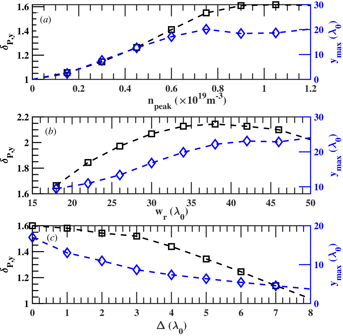
Normalised standard deviation of the poloidal power distribution,
 $\delta _{P,y}$
(black), and shift of the maximum emission position,
 ${y}_{max }$
(blue), as functions of filament parameters at
 $f_{0}=40{\rm GHz}$
: (a) peak density scan, (b) width scan and (c) beam-axis displacement scan. Here,
 $\delta _{P,y}$
is normalised to the standard deviation in the no-ELM reference case and is therefore dimensionless.

Snapshots of the electric-field structure for the parameter scans at fixed
 $n_{peak}=8\times 10^{18}\,{\rm m}^{-3}$
. Panels (a1)–(a3) show the width scan for
 $w_{r}=16\lambda _{0}$
,
 $26\lambda _{0}$
and
 $36\lambda _{0}$
, respectively. Panels (b1)–(b3) show the beam-axis displacement scan for
 $\varDelta$
 $=1\lambda _{0}$
,
 $3\lambda _{0}$
and
 $6\lambda _{0}$
, respectively. All panels are plotted using the same vertical scale for direct comparison.

Figure 5. Long description
Panel A1: A heat map showing the electric-field structure for a width scan with specific parameters. The x-axis is labeled x (λ_0) ranging from 40 to 100, and the y-axis is labeled y (λ_0) ranging from -20 to 20. The color scale on the right indicates values from -1 to 1, with blue representing lower values and red representing higher values. The heat map shows concentric patterns with varying intensities. Panel A2: A heat map showing the electric-field structure for a width scan with different parameters. The axes and color scale are the same as in Panel A1. The patterns are similar but with slight variations in intensity and distribution. Panel A3: A heat map showing the electric-field structure for a width scan with another set of parameters. The axes and color scale remain consistent. The patterns continue to show concentric shapes with different intensity distributions. Panel B1: A heat map displaying the electric-field structure for a beam-axis displacement scan with specific parameters. The axes and color scale are the same as in the previous panels. The patterns show a shift in the concentration of intensities. Panel B2: A heat map showing the electric-field structure for a beam-axis displacement scan with different parameters. The axes and color scale remain consistent. The patterns exhibit further shifts and variations in intensity. Panel B3: A heat map displaying the electric-field structure for a beam-axis displacement scan with another set of parameters. The axes and color scale are the same. The patterns show additional shifts and changes in intensity distribution.
Figure 4 provides quantitative measures of the filament-induced modification of the reflected beam on the detection plane. Here,
 $\delta _{P,y}$
denotes the normalised standard deviation of the poloidal power distribution and characterises beam broadening and redistribution, while
 ${y}_{max }$
denotes the shift of the maximum emission position and characterises the displacement of the dominant reflected beam. These quantities are used here as practical indicators of beam distortion and beam deflection, rather than as formal measures of scattering cross-section or scattering angle.
Figure 4(a) shows
 $\delta _{P,y}$
and
 ${y}_{max }$
as functions of the filament peak density
 $n_{peak}$
, with the other filament parameters fixed. Both
 $\delta _{P,y}$
and
 ${y}_{max }$
increase with
 $n_{peak}$
, indicating that the reflected beam becomes increasingly broadened and displaced as the local total density at the filament approaches the O-mode cutoff density corresponding to the probing frequency. In the present case, the incident frequency is
 $f_{0}=40\,{\rm GHz}$
, giving
 $n_{cut}\approx 2.0\times 10^{19}\,{\rm m}^{-3}$
. Once this cutoff condition is exceeded, the response tends to saturate. Since the filament perturbation is prescribed and time-independent and the plasma response is treated as linear in the present model, this trend should be interpreted as a saturation of the linear wave-response geometry rather than as evidence of a nonlinear filament dynamics.
Figure 4(b) shows that increasing filament width leads to larger
 $\delta _{P,y}$
and
 ${y}_{max }$
, indicating stronger beam deflection and a larger modification of the effective reflection geometry. For widths varied from
 $18\lambda _{0}$
to
 $50\lambda _{0}$
at fixed
 $n_{peak}=8\times 10^{18}\,{\rm m}^{-3}$
, the response increases up to
 $w_{r}\sim 35\lambda _{0}$
, after which it tends to saturate. The corresponding field patterns are shown in figure 5(a1)–(a3).
The effect of beam-axis offset was examined by shifting the filament centre relative to the probing beam. As shown in figure 4(c), the beam-axis displacement mainly modifies the symmetry and location of the reflected pattern, while producing a comparatively weaker change in the beam-broadening metric. For
 $n_{peak}=8\times 10^{18}\,{\rm m}^{-3}$
and
 $w_{r}\sim 30\lambda _{0}$
, the symmetric double maxima collapse into a more asymmetric single-peak response as the filament moves off-axis. The peak then drifts toward the beam centre and slightly overshoots at larger offsets. Although the far-off-axis response resembles the unperturbed beam, residual asymmetries remain in the profile and may retain information on filament position near the LCFS. The corresponding field patterns are shown in figure 5(b1)–(b3).
The IF spectral changes discussed here arise from changes in propagation delay and switching between dominant return paths as the filament modifies the cutoff topology, rather than from Doppler shifts associated with filament motion. In this sense, figure 4 provides the quantitative summary of the response trends, while figure 5 visualises the corresponding field structures.
In summary, the parameter scans show that (i) filament peak density mainly controls the overall strength of the reflected response and that the response saturates once the cutoff condition is exceeded; (ii) filament width strongly affects beam deflection and the effective reflection geometry within the present model; and (iii) filament displacement mainly alters the symmetry and location of the reflecting maxima, thereby modifying the reflected pattern in a distinguishable way.
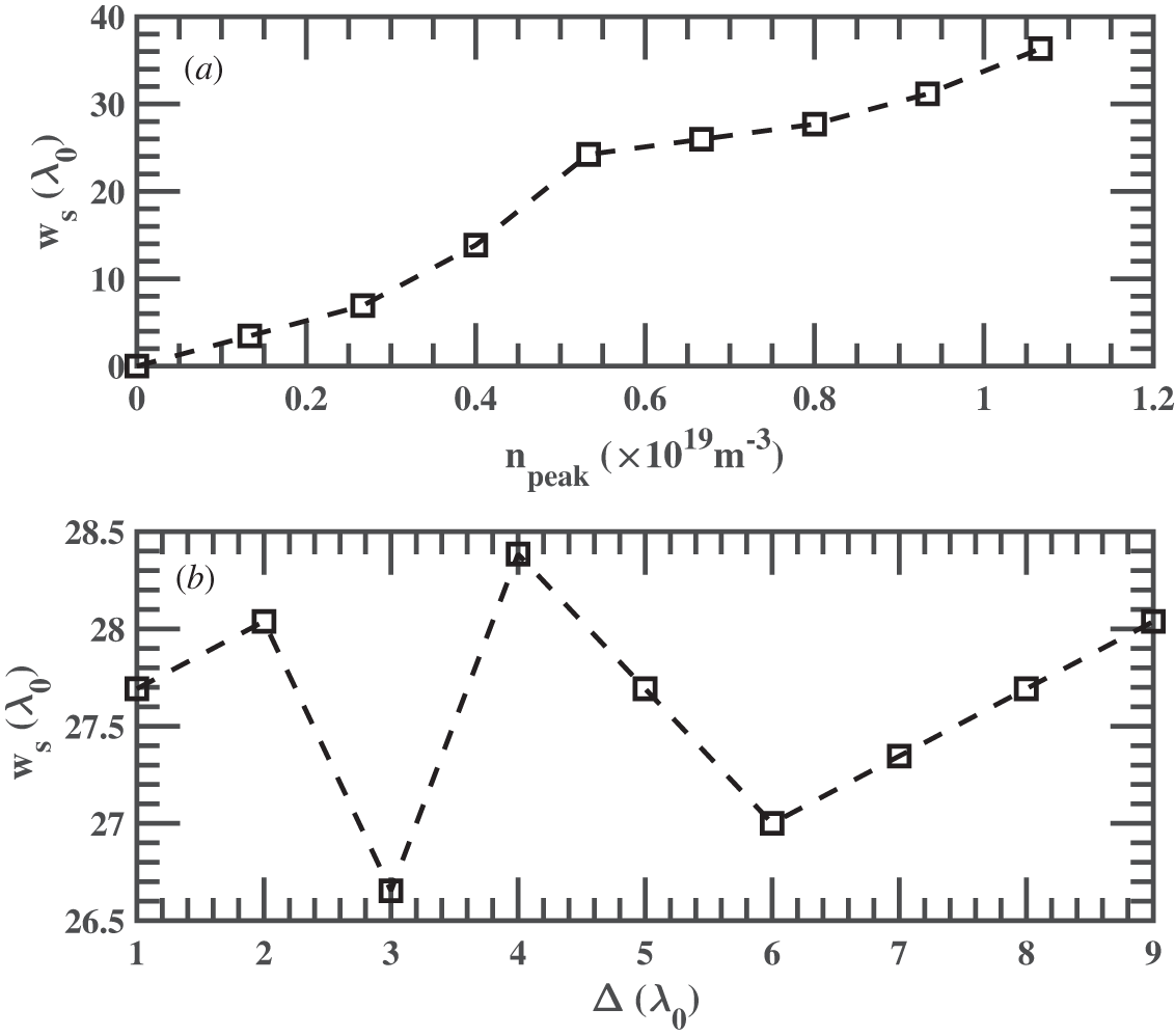
When the filament peak density approaches or exceeds the cutoff density corresponding to the probing frequency, the simulated IF spectrum may exhibit two dominant return branches. This behaviour reflects the formation of two effective reflection paths caused by the filament-modified cutoff topology. To quantify the simulated hopping response, we define a model-derived effective radial scale from the hopping interval between the two dominant IF branches,
 $w_{s}\equiv {\int }_{f_{1}}^{f_{2}}c/(2{S}N_{e{\kern-1.2pt}f{\kern-2.3pt}f}){\rm d}f$
, where
 $f_{1}$
and
 $f_{2}$
are the two dominant IF frequencies identified from the spectral maxima of the main hopping event, S is the FMCW sweep rate and
 $N_{e{\kern-1.2pt}f{\kern-2.3pt}f}$
is an effective refractive-index factor used to account for wave propagation in the plasma. This definition follows the FMCW relation between IF frequency and round-trip propagation delay, but it is used here only as a simulation diagnostic. It should not be interpreted as an experimentally calibrated measurement of the true filament width.
Figure 6(a) shows that
 $w_{s}$
increases with the prescribed filament peak density and tends to approach the imposed filament radial width
 $w_{r}$
in the strong-perturbation regime of the present model. Figure 6(b) shows that the beam-axis displacement has only a weak influence on
 $w_{s}$
. The two frequencies
 $f_{1}$
and
 $f_{2}$
are identified from the two dominant bright branches in figure 3(b2), namely the persistent spectral maxima defining the main hopping event. Isolated weak or dark features are not included because they do not correspond to persistent dominant return branches.
(a) Model-derived effective radial scale
 $w_{s}$
(
 $w_{r}=30\,\lambda _{0}$
) obtained from the IF hopping interval as a function of filament peak density. (b) Effective width
 $w_{s}$
as a function of beam-axis displacement. Here,
 $w_{s}$
is derived from the two dominant IF hopping frequencies in figure 3(b2) and represents a model-based effective width, whereas
 $w_{r}$
denotes the prescribed filament width in the model.

These results indicate that, within the reduced full-wave model, the IF hopping interval is more sensitive to the effective radial scale of the localised density perturbation than to its beam-axis displacement. This provides a simulation-based sensitivity relation between IF hopping and filament width. However, because the instantaneous filament width, density amplitude, radial location and three-dimensional morphology are not independently measured in the present EAST data, this relation cannot yet be used as a direct experimental calibration of filament width. The EAST observations are therefore used here as a morphology-level consistency check for the occurrence of abrupt IF hopping during the ELM-active phase.
4. Conclusion
In this work, the impact of filamentary perturbations on FMCW reflectometry has been investigated using two-dimensional full-wave simulations, with qualitative comparison with experimental observations on EAST. The simulations show that (i) the reflected response strengthens with filament peak density and saturates once the cutoff condition is exceeded, (ii) the filament width strongly affects beam deflection and the effective reflection geometry and (iii) the beam-axis displacement modifies the symmetry and location of the reflected field pattern. These effects manifest in the IF spectrum as multiple peaks and frequency hopping, in qualitative agreement with EAST measurements during ELM events.
Although the present comparison is qualitative rather than quantitative, the similarity in signal morphology between simulation and experiment is consistent with the interpretation of IF hopping as a filament-induced effect. In the present model, the hopping interval is more sensitive to filament width than to filament displacement, indicating that IF hopping contains information on the effective radial scale of the perturbation within the present model. This implication should not be interpreted as a direct quantitative experimental width estimate and will require future validation against independent measurements of filament size.
Overall, these findings highlight the potential of FMCW reflectometry to probe the filament-related dynamics in the pedestal region. Beyond its conventional role in density profile reconstruction, FMCW reflectometry may also provide complementary information for monitoring ELM-related filamentary perturbations. Since the present study is based on a reduced slab model intended for mechanism identification, future work will extend the analysis toward more realistic device geometry, antenna configuration and closer quantitative validation against EAST measurements.
Acknowledgements
Editor Eleonora Viezzer thanks the referees for their advice in evaluating this article.
Funding
This work was supported by the Natural Science Research Project of the Anhui Educational Committee (Grant Nos. 2023AH050501, 2023AH050491).
Declaration of interests
The authors report no conflict of interest.

 ne0(x)
 nfil(x,y)
 δne
 ne(x,y)=ne0(x)+nfil(x,y)+δne(x,y)


 δP,y
 ymax
 f0=40GHz
 δP,y

 npeak=8×10¹⁸m−3
 wr=16λ0
 26λ0
 36λ0
 Δ
 =1λ0
 3λ0
 6λ0
 ws
 wr=30λ0
 ws
 ws
 wr

 Open access

