



1. Introduction
Let
 $\mathbb{N}\;:\!=\;\{0,1,2,\ldots\}$
. We consider a continuous-time model in
 $D\;:\!=\;\mathbb{R}_+\times\mathbb{N}$
for cells and parasites, where the behavior of the cell division is affected by the parasites. We assume that the parasites proliferate in the cells, and their life-lengths are much less than that of the cells. Informally, the quantity of parasites
 $(X(t))_{t\geq0}$
in cells evolves as a continuous-state branching process (CB-process for short); see [Reference Dawson and Li9, Reference Dawson and Li10, Reference Kyprianou19, Reference Li25] for more details of such processes. Denote the number of cells by
 $(Y(t))_{t\geq0}$
. Cells divide in continuous time at a rate h(x, y) that may depend on the number of parasites x and cells y, and then give birth to a random number of offspring, with the same offspring distribution independent of x and y. This framework is general enough to be applied in modeling other structured populations, e.g. grass–rabbit models in [Reference Ji and Xiong17].
Many studies have been conducted on branching within branching processes to study such population dynamics in continuous time. In [Reference Osorio and Winter32], the evolution of parasites is modeled by a birth–death process, while the cells split according to a Yule process. [Reference Bansaye and Tran3] allows the number of parasites in a cell to follow a Feller diffusion. A general CB-process is considered to model the number of parasites in a cell in [Reference Marguet and Smadi31]. In particular, [Reference Bansaye and Tran3, Reference Marguet and Smadi31, Reference Osorio and Winter32] describe cell populations using a tree-structure model. In this way, the cell population can be represented by a random point-measure-valued process, and the associated martingale problem can be formulated by choosing test functions appropriately. We also refer to [Reference Bansaye and Tran3, Reference Marguet and Smadi31, Reference Osorio and Winter32] and the references therein for the biological motivation and experimental support. It is well known that a supercritical CB-process is equal in law to a continuous-time branching process (the skeleton of prolific individuals), where the edges are decorated in a Poissonian way with immigration, which initiates subcritical CB-processes; see, e.g., [Reference Berestycki, Kyprianou and Murillo-Salas4, Reference Bertoin, Fontbona and Martinez5, Reference Duquesne and Winkel11]. In the spirit of [Reference Duquesne and Winkel11, Reference Feketa, Fontbona and Kyprianou13] provided a slightly more general family of skeletal decompositions by using the framework of coupled stochastic differential equations (SDEs). After that, a mixed-state and continuous-time branching process in D satisfying the branching property (see, e.g., [Reference Li26, p. 6, (9)]) was constructed by a scaling method in [Reference Chen and Li7]. For this model, the first component can be seen as a CB-process affected by the second one, and the second component with state space
 $\mathbb{N}$
can also be seen as a continuous-time branching process affected by the first one.
Inspired by [Reference Chen and Li7], in this paper we ignore the tree structure and mainly focus on a parasite–cell model from a macro point of view. More precisely, we use a stochastic equation system to describe the sample path of such models. Let
 $B=(B(t))_{t \ge 0}$
be a standard Brownian motion,
 $(\xi\wedge \xi^2)\,m({\mathrm{d}} \xi)$
be a finite measure on
 $(0, \infty)$
, and
 $(p_\xi,\xi\in\mathbb{N})$
be an offspring distribution satisfying
 $\sum_\xi \xi p_\xi<\infty$
. Without losing generality, we assume
 $p_1 = 0$
. Let
 $M({\mathrm{d}} s, {\mathrm{d}} u, {\mathrm{d}} \xi)$
be a Poisson random measure on
 $(0, \infty)^3$
with intensity
 ${\mathrm{d}} s\,{\mathrm{d}} u\,m({\mathrm{d}} \xi)$
, and
 $\tilde{M}({\mathrm{d}} s,{\mathrm{d}} u,{\mathrm{d}} \xi)=M({\mathrm{d}} s,{\mathrm{d}} u,{\mathrm{d}} \xi)-{\mathrm{ d}} s\,{\mathrm{d}} u\,m({\mathrm{d}} \xi)$
. Define
 $N_0$
to be a Poisson random measure on
 $(0, \infty)^3\times\mathbb{N}$
with intensity
 ${\mathrm{d}} s\,{\mathrm{d}} u\,{\mathrm{d}} r\,n_0({\mathrm{d}} \xi)$
, where
 $n_0({\mathrm{d}} \xi) = p_\xi\sharp({\mathrm{d}}\xi)$
and
 $\sharp(\cdot)=\sum_j\delta_j(\cdot)$
is the counting measure on
 $\mathbb{N}$
. Moreover, we assume the three random elements B, M, and
 $N_0$
are defined on a completed probability space and are independent of each other. Consider the following stochastic equation system:
 \begin{equation*} \begin{cases} X(t)=X(0)-b\displaystyle\int_0^t X(s)\,{\mathrm{d}} s+\displaystyle\int_0^t\sqrt{2cX(s)}\,{\mathrm{d}} B(s)+\displaystyle\int_0^t\displaystyle\int_0^{X(s-)}\displaystyle\int_0^\infty \xi\,\tilde{M}({\mathrm{d}} s,{\mathrm{d}} u,{\mathrm{d}} \xi),\\[9pt] Y(t)=Y(0)+\displaystyle\int_0^t\displaystyle\int_0^{Y(s-)}\displaystyle\int_0^{h(X(s-),Y(s-))}\displaystyle\int_{ \mathbb{N}} (\xi-1)\,N_0({\mathrm{d}} s,{\mathrm{d}} u,{\mathrm{d}} r,{\mathrm{d}} \xi), \end{cases}\end{equation*}
where
 $b \in \mathbb{R}$
and
 $c\geq0$
are constants, and
 $h(\cdot,\cdot)\in C(D)^+$
, which is the collection of all non-negative functions
 $(x, y)\mapsto f(x, y)$
on D with
 $x \mapsto f(x, \cdot)$
being continuous. It is easy to see that
 $(X(t))_{t\geq0}$
is indeed a CB-process, and
 $(Y(t))_{t\geq0}$
is a continuous-time branching-type process affected by
 $(X(t))_{t\geq0}$
. Clearly,
 $(X(t),Y(t))_{t\geq0}$
fails to satisfy the branching property unless h is a constant function.
For simplicity, we introduce another Poisson random measure
 $N({\mathrm{d}} s, {\mathrm{d}} u, {\mathrm{d}} r, {\mathrm{d}} \xi)$
on
 $(0,\infty)^3\times\mathbb{N}^{-1}$
with intensity measure
 ${\mathrm{d}} s\,{\mathrm{d}} u\,{\mathrm{ d}} r\,n({\mathrm{d}}\xi)$
, where
 $\mathbb{N}^{-1}=\mathbb{N}\cup\{-1\}$
,
 $n({\mathrm{d}}\xi)=p_{\xi+1}\sharp({\mathrm{d}} \xi)$
, and
 $\sharp({\mathrm{d}} \xi)$
is the counting measure on
 $\mathbb{N}^{-1}$
. Then we can rewrite the system by
 \begin{align} & \qquad\qquad\qquad\qquad\qquad\qquad\qquad\qquad\qquad\qquad\qquad\qquad\qquad\qquad\qquad\qquad\qquad\quad\;\; (1.1) \nonumber \\[-22pt]&\! \left\{\begin{array}{l}X(t)=X(0)-b\displaystyle\int_0^t X(s)\,{\mathrm{d}} s+\displaystyle\int_0^t\sqrt{2cX(s)}\,{\mathrm{d}} B(s)+\displaystyle\int_0^t\displaystyle\int_0^{X(s-)}\displaystyle\int_0^\infty \xi\,\tilde{M}({\mathrm{d}} s,{\mathrm{d}} u,{\mathrm{d}} \xi),\\[9pt] Y(t)=Y(0)+\displaystyle\int_0^t\displaystyle\int_0^{Y(s-)}\displaystyle\int_0^{h(X(s-),Y(s-))}\displaystyle\int_{\mathbb{N}^{-1}} \xi\,N({\mathrm{d}} s,{\mathrm{d}} u,{\mathrm{d}} r,{\mathrm{d}} \xi).\end{array} \right.\nonumber \\[-21pt]& \qquad\qquad\qquad\qquad\qquad\qquad\qquad\qquad\qquad\qquad\qquad\qquad\qquad\qquad\qquad\qquad\qquad\quad\;\; (1.2) \nonumber \end{align}
In the rest of the paper we use the stochastic equation system (1.1) and (1.2) to describe the parasite–cell model. In the literature on the theory of branching processes, the rescaling (in time or state) approach plays a valuable role in establishing the connection among those branching processes – see [Reference Chen and Li7, Reference Kawazu and Watanabe18, Reference Li24, Reference Li25, Reference Liu28, Reference Ma30] and the references therein. To the best of our knowledge, limited work has been done in branching processes with interactions. This leads to the first goal of this paper: the establishment of weak existence and pathwise uniqueness of the solution to (1.1)and (1.2). For a sequence of two-type Galton–Watson processes with interactions
 $\{(x_k(n),y_k(n))_{n\in\mathbb{N}}\}_{k\geq1}$
, we prove that
 $(x_k(\lfloor\gamma_kt\rfloor)/k,y_k(\lfloor\gamma_kt\rfloor))_{t\geq0}$
converges in distribution to the solution to (1.1) and (1.2) as
 $k \rightarrow \infty$
under suitable conditions. The pathwise uniqueness of the solution to (1.1) and (1.2) is also given.
In addition, the second goal of this paper is to study long-time behaviors of such processes, with a particular focus on the extinction behavior and exponential ergodicity in the
 $L^1$
-Wasserstein distance in certain cases. The result of extinction behavior is inspired by [Reference Li, Yang and Zhou23]. Furthermore, ergodicity is the foundation for a wide class of limit theorems and long-time behavior for Markov processes. Due to the nonlinearity of the function h, the semigroup transition of (X, Y) is not explicit. We obtain the ergodic property by a coupling approach, which has been proved to be effective in the study of ergodicity of the nonlinear case; see [Reference Chen6, Reference Luo and Wang29] and the references therein.
We now introduce some notation. Let
 ${\mathrm{e}}_\lambda(z) \;:\!=\;{\mathrm{e}}^{-\langle \lambda, z\rangle}$
for any
 $\lambda = (\lambda_1, \lambda_2) \in \mathbb{R}_+^2$
and
 $z=(x, y) \in D$
, where
 $\langle \lambda, z\rangle = \lambda_1 x + \lambda_2 y$
. We use
 $C_\mathrm{b}(D)^+$
to denote the set of all bounded non-negative functions
 $(x, y) \mapsto f(x, y)$
on D with
 $x \mapsto f(x, \cdot)$
continuous. Let
 $C_\mathrm{b}^2(D)^+$
be the subset of
 $C_\mathrm{b}(D)^+$
with continuous bounded derivatives up to the second order of x. Denote by
 $C^2(D)^+$
the subset of
 $C(D)^+$
with continuous derivatives up to the second order of x. Let
 $C_0^2(D)^+$
be the subset of
 $C^2(D)^+$
vanishing at infinity. Let
 ${\mathbb{D}}(\mathbb{R}_+, D)$
denote the space of càdlàg paths from
 $\mathbb{R}_+$
to D furnished with the Skorokhod topology. In the integrals, we make the convention that, for
 $a \le b \in \mathbb{R}$
,
 $\int_a^b = \int_{(a, b]}$
and
 $ \int_a^\infty = \int_{(a, \infty)}$
.
This paper is structured as follows. The existence by a scaling limit of a sequence of two-type Galton–Watson processes with interaction, and the pathwise uniqueness of the solution to (1.1) and (1.2) are given in Section 2. In Section 3 the extinction behavior of the system is studied. In Section 4, an exponential ergodic property is proved under suitable conditions.
2. Existence and pathwise uniqueness of solution
The generator A of
 $(X(t),Y(t))_{t\geq0}$
satisfying (1.1) and (1.2) is determined by
 \begin{align} Af(z) & = x\bigg[{-}bf'_x+cf''_{xx} + \displaystyle\int_0^\infty\{f(x+\xi,y)-f(x,y)-\xi f'_x\}\, m({\mathrm{d}}\xi)\bigg] \cr & \quad + \gamma(x,y)\displaystyle\int_{\mathbb{N}^{-1}}\{f(x,y+\xi)-f(x,y)\}\,n({\mathrm{d}}\xi) \end{align}
for any
 $z = (x, y) \in D$
and
 $f\in \mathcal{D}(A)$
, where
 $\gamma(x, y) = h(x, y)y$
, and
 $\mathcal{D}(A)$
denotes the linear space consisting of functions
 $f\in C^{2}(D)^+$
such that the two integrals on the right-hand side of (2.1) are convergent and define continuous functions on D. Then
 \begin{equation} A\mathrm{e}_\lambda(z) = \mathrm{e}_\lambda(z)[x\phi_1(\lambda_1)+\gamma(x,y)\phi_2(\lambda_2)],\end{equation}
where
 \begin{align} \phi_1(\lambda_1) & = b\lambda_1 + c\lambda_1^2 + \displaystyle\int_0^\infty\big(\mathrm{e}^{-\lambda_1\xi}-1+\lambda_1\xi\big)\, m({\mathrm{d}}\xi), \end{align}
 \begin{align} \phi_2(\lambda_2) = \displaystyle\int_{\mathbb{N}^{-1}}(\mathrm{e}^{-\lambda_2\xi}-1)\,n({\mathrm{d}}\xi).\qquad\qquad\;\;\; \end{align}
We first consider the case of
 $h \in C_\mathrm{b}(D)^+$
. Given the initial value
 $(x(0),y(0))\in\mathbb{N}\times\mathbb{N}$
, let
 $(x(n),y(n))_{n\ge 0}$
be a two-dimensional process defined by
 \begin{equation*} x(n) \;:\!=\; \sum_{j=1}^{x(n-1)}\alpha_{n-1,j}, \qquad y(n) \;:\!=\; \sum_{j=1}^{y(n-1)}\beta_{n-1,j,\theta(x(n-1),y(n-1))}, \quad n\geq1,\end{equation*}
where
 $\{\alpha_{n,j}\colon n\geq 0,j\geq1\}$
are integer-valued independent and identically distributed (i.i.d.) random variables with offspring distribution
 $(w(i)\colon i\in\mathbb{N})$
. Given
 $x,y \in \mathbb{N}$
, the above
 $\{\beta_{n,j,\theta(x,y)}\colon n\geq 0,j\geq1\}$
are i.i.d. integer-valued random variables with offspring distribution
 $(v^{\theta(x,y)}(i)\colon i\in\mathbb{N})$
depending on the function
 $\theta$
. Let
 $g_1$
and
 $g^{\theta(x,y)}_2$
be the generating functions of
 $(w(i)\colon i\in\mathbb{N})$
and
 $(v^{\theta(x,y)}(i)\colon i\in\mathbb{N})$
, respectively. It is known that
 $(x(n), y(n))_ {n\geq0}$
is a Markov process and we call it a two-type Galton–Watson process with interaction. Suppose that there exists a sequence of two-type Galton–Watson processes with interaction
 $\{(x_k(n),y_k(n))_{n\geq0}\}_{k\geq1}$
with parameters
 $(g_{k,1},g_{k,2}^{\theta_k(x,y)})$
. Let
 $\{\gamma_k\}_{k\geq1}$
be a sequence of positive numbers with
 $\gamma_k \rightarrow \infty$
as
 $k \rightarrow \infty$
. For
 $(x, y) \in \mathbb{N}\times\mathbb{N}$
, we introduce several functions on
 $\mathbb{R}_+$
:
 \begin{align*} \bar{\Phi}_{k,1}(\lambda_1) & \;:\!=\; k\gamma_k\log\big[1-(k\gamma_k)^{-1}\Phi_{k,1}(\lambda_1)\mathrm{e}^{\lambda_1/k}\big], \\[5pt] \Phi_{k,1}(\lambda_1) & \;:\!=\; k\gamma_k\big[\mathrm{e}^{-\lambda_1/k}-g_{k,1}(\mathrm{e}^{-\lambda_1/k})\big], \\[5pt] \bar{\Phi}_{k,2}^{\theta_k(x,y)}(\lambda_2) & \;:\!=\; \gamma_k\log\big[1-\gamma_k^{-1}\Phi_{k,2}^{\theta_k(x,y)}(\lambda_2)\mathrm{e}^{\lambda_2}\big], \\[5pt] \Phi_{k,2}^{\theta_k(x,y)}(\lambda_2) & \;:\!=\; \gamma_k\big[\mathrm{e}^{-\lambda_2}-g_{k,2}^{\theta_k(x,y)}(\mathrm{e}^{-\lambda_2})\big].\end{align*}
Let
 $E_k \;:\!=\; \{0, k^{-1}, 2k^{-1}, \ldots\}$
for each
 $k\geq1$
. For any
 $x \in \mathbb{R}_+$
, we take
 $x_k \;:\!=\; \lfloor kx\rfloor/k$
. Then
 $x_k \in E_k$
and
 $|x_k - x| \le 1/k$
. Let
 $D_k\;:\!=\; E_k \times \mathbb{N}$
, which is a subset of D. We define a continuous-time stochastic process taking values on
 $D_k$
as
 $(X_k(t), Y_k(t))_{t \ge 0}\;:\!=\;(x_k(\lfloor \gamma_k t\rfloor)/k,y_k(\lfloor \gamma_k t\rfloor))_{t\geq0}$
. Write
 $Z_k(t) \;:\!=\; (X_k(t), Y_k(t))$
to simplify the notation. In order to state our main results, we first present the following condition assumed throughout this section.
Condition 2.1.
-
(C1) The sequence
 $\{\Phi_{k,1}(\lambda_1)\}_{k \ge 1}$
is uniformly Lipschitz in
$\lambda_1$
on each bounded interval, and converges to a continuous function as
$k \rightarrow \infty$
;
-
(C2)
$\gamma_k\big[1- v_k^{\theta_k(kx_k,y)}(1)\big] \rightarrow h(x, y)$
uniformly in
$(x, y) \in D$
as
$k \rightarrow \infty$
; -
(C3)
$\dfrac{v_k^{\theta_k(kx_k, y)}(\xi)}{1- v_k^{\theta_k(kx_k,y)}(1)} \rightarrow p_\xi$
for
$\xi \in \mathbb{N}\backslash \{1\}$
uniformly in
$(x, y) \in D$
as
$k \rightarrow \infty$
; -
(C4) The sequence
$\big\{\Phi_{k,2}^{\theta_k(kx_k,y)}(\lambda_2)\big\}_{k \ge 1}$
is uniformly Lipschitz in
$\lambda_2$
on each bounded interval, where the Lipshcitz coefficient does not depend on x and y.


By [Reference Li26, Proposition 2.5], under (C1) of Condition 2.1,
 $\Phi_{k,1}(\lambda_1)$
converges to a function
 $\phi_1(\lambda_1)$
with representation (2.3) as
 $k \rightarrow \infty$
; see also [Reference Li24, Reference Li25]. Moreover, there exists a constant
 $K > 0$
such that
 \begin{equation} \sup_k\Phi_{k,1}'(0+) = \sup_k \gamma_k[g_{k,1}'(1-\!) - 1] \le K.\end{equation}
Example 2.1. Let
 $\{p_\xi\colon\xi = 0,1,\ldots\}$
be an offspring distribution with
 $p_1 = 0$
and
 $h \in C_\mathrm{b}(D)^+$
. Let
 \begin{align*} v_k^{\theta_k(kx_k, y)}(\xi) & \;:\!=\; p_\xi\gamma_k^{-1/2}\big(1 - {\mathrm{e}}^{-\gamma_k^{-1/2}h(x_k, y)}\big) \quad \text{for any } \xi \in \mathbb{N}\backslash \{1\}, \\[5pt] v_k^{\theta_k(kx_k, y)}(1) & \;:\!=\; 1 - \gamma_k^{-1/2}\big(1 - {\mathrm{e}}^{-\gamma_k^{-1/2}h(x_k, y)}\big). \end{align*}
Then
 $\Phi_{k,2}^{\theta_k(kx_k,y)}(\lambda_2) = \gamma_k^{1/2}\big(1 - {\mathrm{e}}^{-\gamma_k^{-1/2}h(x_k, y)}\big) (\mathrm{e}^{-\lambda_2}-g(\mathrm{e}^{-\lambda_2}))$
with
 $g(\mathrm{e}^{-\lambda_2}) = \sum_{\xi= 0}^\infty p_\xi{\mathrm{e}}^{-\lambda_2\xi}.$
We can check that this satisfies (C2)–(C1) of Condition 2.1.
2.1. Main results
We now proceed to present the main results about a scaling limit theorem for mixed-state branching processes with interactions, and the existence and pathwise uniqueness of the solution to (1.1) and (1.2).
Theorem 2.1. Suppose that Condition 2.1 holds and
 $h \in C_\mathrm{b}(D)^+$
. Let
 $Z_k(0)$
converge in distribution to Z(0) as
 $k \rightarrow \infty$
, with
 $\sup_k \mathbb{E}[X_k(0) + Y_k(0)] < \infty$
. Then
 $\{(Z_k(t))_{ t \ge 0}\}_{k \ge 1}$
converges in distribution on
 ${\mathbb{D}}(\mathbb{R}_+, D)$
to
 $(Z(t))_{t \ge 0}$
, which is a solution to (1.1) and (1.2).
Theorem 2.2. Assume that
 $h \in C_\mathrm{b}(D)^+$
. For any given initial value
 $(X(0),Y(0))\in D$
, pathwise uniqueness holds for (1.1) and (1.2) on D.
Remark 2.1. For the classical branching process, the transition semigroup can be determined uniquely by the log-Laplace transform because of the branching property. Then the linear span of
 $\{{\mathrm{e}}^{-\lambda x}\colon\lambda \ge 0\}$
forms the core of the generator of the process. Therefore, the scaling limit theorem can be obtained in the sense of convergence in distribution on the Skorokhod space by [Reference Ethier and Kurtz12, pp. 226, 233–234]. We refer to [Reference Kawazu and Watanabe18, Reference Li24] and the references therein for details. However, the branching property is invalid for our model because of the interaction. It is not enough to give only the estimation when
 $f = {\mathrm{e}}_\lambda$
. Therefore, in the following proof of Theorem 2.1 we show the existence of a solution to the martingale problem by tightness for general f. Then, by the representation theorem for semimartingales (see, e.g., [Reference Ikeda and Watanabe16, pp. 90, 93]), we have the equation system (1.1) and (1.2) on an extension of the original probability space, which proves the existence of a weak solution to (1.1) and (1.2).
As we know, there is a unique strong solution to (1.1), which is a CB-process. Based on this, in the proof of Theorem 2.2 we construct the pathwise unique solution to (1.2) by the method of concatenating paths.
There is a unique positive strong solution to (1.1) and(1.2) by Theorems 2.1 and 2.2 when
 $h \in C_\mathrm{b}(D)^+$
. However, the boundedness assumption of h can be removed, which is given in the following result.

2.2. Proofs of main results
In this section, we prove Theorem 2.1 by tightness at first. Then Theorem 2.2 is proved by the method of concatenating paths. Based on these results, the proof of Theorem 2.3 is given.
For the proof of Theorem 2.1, we demonstrate the existence of a solution to the martingale problem by proving tightness for
 $f = {\mathrm{e}}_\lambda$
, and then extend the result for general f.
For
 $\lambda = (\lambda_1, \lambda_2) \in \mathbb{R}_+^2$
, let
 \begin{align} M_{k,\lambda}(t) & \;:\!=\; \sum_{i=1}^{\lfloor\gamma_kt\rfloor}\bigg\{\bigg[ {\mathrm{e}}_\lambda\bigg(Z_k\bigg(\frac{i}{\gamma_k}\bigg)\bigg) - {\mathrm{e}}_\lambda\bigg(Z_k\bigg(\frac{i-1}{\gamma_k}\bigg)\bigg)\bigg] \cr & \qquad\qquad - \mathbb{E}\bigg[{ \mathrm{e}}_\lambda\bigg(Z_k\bigg(\frac{i}{\gamma_k}\bigg)\bigg) - {\mathrm{e}}_\lambda\bigg(Z_k\bigg(\frac{i-1}{\gamma_k}\bigg)\bigg) \mid \mathscr{F}_{({i-1})/{\gamma_k}}\bigg]\bigg\}.\end{align}
Moreover, for
 $z = (x, y) \in D$
, let
 \begin{equation} A_k\mathrm{e}_\lambda(z) \;:\!=\; \gamma_k\big[(g_{k,1}(\mathrm{e}^{-\lambda_1/k}))^{ kx_k} \cdot \big(g_{k,2}^{ \theta_k(kx_k,y)}({\mathrm{e}}^{-\lambda_2})\big)^y - \mathrm{e}_\lambda(z)\big].\end{equation}
We can check that
 \begin{equation} A_k\mathrm{e}_\lambda(z) = \mathrm{e}_\lambda(z)\big[x\bar{\Phi}_{k,1}(\lambda_1) + y\bar{\Phi}_{k,2}^{\theta_k(kx_k,y)}(\lambda_2)\big] + o(1).\end{equation}
By the definition of
 $(Z_k(t))_{t \ge 0}$
and (2.7), we can see that
 $Z_k(t) = Z_k(\lfloor \gamma_k t\rfloor/\gamma_k)$
and
 \begin{equation} \mathbb{E}\bigg[{\mathrm{e}}_\lambda\bigg(Z_k\bigg(\frac{i}{\gamma_k}\bigg)\bigg) - {\mathrm{e}}_\lambda\bigg(Z_k\bigg(\frac{i-1}{\gamma_k}\bigg)\bigg) \mid \mathscr{F}_{({i-1})/{\gamma_k}}\bigg] = \gamma_k^{-1}A_k {\mathrm{e}}_\lambda\bigg(Z_k\bigg(\frac{i-1}{\gamma_k}\bigg)\bigg).\end{equation}
Then we have
 \begin{align} {\mathrm{e}}_\lambda(Z_k(t)) & = {\mathrm{e}}_\lambda(Z_k(0)) + \sum_{i=1}^{\lfloor\gamma_kt\rfloor}\bigg[ {\mathrm{e}}_\lambda\bigg(Z_k\bigg(\frac{i}{\gamma_k}\bigg)\bigg) - {\mathrm{e}}_\lambda\bigg(Z_k\bigg(\frac{i-1}{\gamma_k}\bigg)\bigg)\bigg] \cr & = {\mathrm{e}}_\lambda(Z_k(0)) + \sum_{i=1}^{\lfloor\gamma_kt\rfloor}\gamma_k^{-1}A_k {\mathrm{e}}_\lambda\bigg(Z_k\bigg(\frac{i-1}{\gamma_k}\bigg)\bigg) + M_{k,\lambda}(t) \cr & = {\mathrm{e}}_\lambda(Z_k(0)) + \displaystyle\int_0^{\lfloor\gamma_kt\rfloor/\gamma_k}A_k{\mathrm{e}}_\lambda(Z_k(s))\, {\mathrm{d}}s + M_{k,\lambda}(t). \end{align}
Lemma 2.1. The variation process of
 $M_{k,\lambda}(t)$
is
 \begin{equation*} \langle M_{k,\lambda}\rangle(t) = \displaystyle\int_0^{\lfloor\gamma_kt\rfloor/\gamma_k} \big[A_k{\mathrm{e}}_{2\lambda}(Z_k(s)) - 2{\mathrm{e}}_\lambda(Z_k(s))A_k{\mathrm{e}}_\lambda(Z_k(s))\big]\, {\mathrm{d}}s + O(\gamma_k^{-1}). \end{equation*}
Proof. By (2.9), we can see that
 \begin{align*} & \mathbb{E}\bigg[\bigg[{\mathrm{e}}_\lambda\bigg(Z_k\bigg(\frac{i}{\gamma_k}\bigg)\bigg) - {\mathrm{e}}_\lambda\bigg(Z_k\bigg(\frac{i-1}{\gamma_k}\bigg)\bigg)\bigg]^2 \mid \mathscr{F}_{({i-1})/{\gamma_k}}\bigg] \cr & \quad = \mathbb{E}\bigg[{\mathrm{e}}_{2\lambda}\bigg(Z_k\bigg(\frac{i}{\gamma_k}\bigg)\bigg) \mid \mathscr{F}_{({i-1})/{\gamma_k}}\bigg] - 2{\mathrm{e}}_\lambda\bigg(Z_k\bigg(\frac{i-1}{\gamma_k}\bigg)\bigg) \mathbb{E}\bigg[{\mathrm{e}}_{\lambda}\bigg(Z_k\bigg(\frac{i}{\gamma_k}\bigg)\bigg) \mid \mathscr{F}_{({i-1})/{\gamma_k}}\bigg] \cr & \qquad + {\mathrm{e}}_{2\lambda}\bigg(Z_k\bigg(\frac{i-1}{\gamma_k}\bigg)\bigg) \cr & \quad = \mathbb{E}\bigg[{\mathrm{e}}_{2\lambda}\bigg(Z_k\bigg(\frac{i}{\gamma_k}\bigg)\bigg) - {\mathrm{e}}_{2\lambda}\bigg(Z_k\bigg(\frac{i - 1}{\gamma_k}\bigg)\bigg) \mid \mathscr{F}_{({i-1})/{\gamma_k}}\bigg] \cr & \qquad - 2{\mathrm{e}}_\lambda\bigg(Z_k\bigg(\frac{i-1}{\gamma_k}\bigg)\bigg) \mathbb{E}\bigg[{\mathrm{e}}_{\lambda}\bigg(Z_k\bigg(\frac{i}{\gamma_k}\bigg)\bigg) - {\mathrm{e}}_{\lambda}\bigg(Z_k\bigg(\frac{i - 1 }{\gamma_k}\bigg)\bigg) \mid \mathscr{F}_{({i-1})/{\gamma_k}}\bigg] \cr & \quad = \gamma_k^{-1}A_k{\mathrm{e}}_{2\lambda}\bigg(Z_k\bigg(\frac{i-1}{\gamma_k}\bigg)\bigg) - 2{\mathrm{e}}_\lambda\bigg(Z_k\bigg(\frac{i-1}{\gamma_k}\bigg)\bigg)\gamma_k^{-1}A_k {\mathrm{e}}_\lambda\bigg(Z_k\bigg(\frac{i-1}{\gamma_k}\bigg)\bigg). \end{align*}
Then, using this and (2.6), we have
 \begin{align*} \langle M_{k,\lambda}\rangle(t) & = \sum_{i=1}^{\lfloor\gamma_kt\rfloor}\mathbb{E}\Bigg\{\Bigg[\bigg[ {\mathrm{e}}_\lambda\bigg(Z_k\bigg(\frac{i}{\gamma_k}\bigg)\bigg) - {\mathrm{e}}_\lambda\bigg(Z_k\bigg(\frac{i-1}{\gamma_k}\bigg)\bigg)\bigg] \cr & \qquad\qquad - \mathbb{E}\bigg[{\mathrm{e}}_\lambda\bigg(Z_k\bigg(\frac{i}{\gamma_k}\bigg)\bigg) - {\mathrm{e}}_\lambda\bigg(Z_k\bigg(\frac{i-1}{\gamma_k}\bigg)\bigg) \mid \mathscr{F}_{({i-1})/{\gamma_k}}\bigg]\Bigg]^2 \mid \mathscr{F}_{({i-1})/{\gamma_k}}\Bigg\} \cr & = \sum_{i=1}^{\lfloor\gamma_kt\rfloor}\Bigg\{\mathbb{E}\bigg[\bigg[ {\mathrm{e}}_\lambda\bigg(Z_k\bigg(\frac{i}{\gamma_k}\bigg)\bigg) - {\mathrm{e}}_\lambda\bigg(Z_k\bigg(\frac{i-1}{\gamma_k}\bigg)\bigg)\bigg]^2 \mid \mathscr{F}_{({i-1})/{\gamma_k}}\bigg] \cr & \qquad\qquad - \bigg[\mathbb{E}\bigg[{\mathrm{e}}_\lambda\bigg(Z_k\bigg(\frac{i}{\gamma_k}\bigg)\bigg) - {\mathrm{e}}_\lambda\bigg(Z_k\bigg(\frac{i-1}{\gamma_k}\bigg)\bigg) \mid \mathscr{F}_{({i-1})/{\gamma_k}}\bigg]\bigg]^2\Bigg\} \cr & = \sum_{i=1}^{\lfloor\gamma_kt\rfloor}\Bigg\{\gamma_k^{-1}A_k {\mathrm{e}}_{2\lambda}\bigg(Z_k\bigg(\frac{i-1}{\gamma_k}\bigg)\bigg) - 2\mathrm{e}_\lambda\bigg(Z_k\bigg(\frac{i-1}{\gamma_k}\bigg)\bigg)\gamma_k^{-1}A_k {\mathrm{e}}_\lambda\bigg(Z_k\bigg(\frac{i-1}{\gamma_k}\bigg)\bigg) \cr & \qquad\qquad - \gamma_k^{-2}\bigg(A_k{\mathrm{e}}_\lambda\bigg(Z_k\bigg(\frac{i-1}{\gamma_k}\bigg)\bigg)\bigg)^2 \Bigg\} \cr & = \displaystyle\int_0^{\lfloor\gamma_kt\rfloor/\gamma_k}\big[A_k{\mathrm{e}}_{2\lambda}(Z_k(s)) - 2{\mathrm{e}}_\lambda(Z_k(s))A_k{\mathrm{e}}_\lambda(Z_k(s))\big]\,{\mathrm{d}}s + O(\gamma_k^{-1}). \end{align*}
The result follows.
Proposition 2.1. Under (C2) and (C3) of Condition 2.1,
 $\mathrm{e}^{\lambda_2}\Phi^{\theta_k(kx_k,y)}_{k,2}(\lambda_2)$
converges to
 $-h(x,y)$
 $\times\phi_2(\lambda_2)$
uniformly for
 $(x,y,\lambda_2)\in\mathbb{R}_+\times\mathbb{N}\times\mathbb{R}_+$
as
 $k\rightarrow\infty$
, where
 $h \in C_\mathrm{b}(D)^+$
and
 $\phi_2(\lambda_2)$
is given by (2.4).
Proof. We can see that
 \begin{align*} \mathrm{e}^{\lambda_2}\Phi^{\theta_k(kx_k,y)}_{k,2}(\lambda_2) & = \gamma_k\big[1-\mathrm{e}^{\lambda_2}g^{\theta_k(kx_k,y)}_{k,2}(\mathrm{e}^{-\lambda_2})\big] \\[5pt] & = \gamma_k\Bigg[1-\mathrm{e}^{\lambda_2}\sum_{j=0}^{\infty}\mathrm{e}^{-\lambda_2 j}v_k^{\theta_k(kx_k,y)}(j)\Bigg] \cr & = \gamma_k\sum_{j=0}^\infty(1 - {\mathrm{e}}^{-\lambda_2(j-1)})v_k^{\theta_k(kx_k,y)}(j) \cr & = \gamma_k\big[1- v_k^{\theta_k(kx_k,y)}(1)\big]\displaystyle\int_{\mathbb{N}^{-1}\backslash\{0\}} (1-{\mathrm{e}}^{-\lambda_2 \xi})\,\rho_k^{\theta_k(kx_k,y)}({\mathrm{d}}\xi), \end{align*}
where, for
 $\xi \in \mathbb{N}^{-1}\backslash\{0\}$
,
 \begin{align*} \rho^{\theta_k(kx_k,y)}_{k}({\mathrm{d}} \xi) & = \frac{1}{1-v_k^{\theta_k(kx_k,y)}(1)}\sum_{j=0}^\infty v_k^{\theta_k(kx_k,y)}(j)\,\delta_{j-1}({\mathrm{d}}\xi) \cr & = \frac{1}{1-v_k^{\theta_k(kx_k,y)}(1)}\sum_{j=-1}^\infty v_k^{\theta_k(kx_k,y)}(j+1)\,\delta_{j}({\mathrm{d}}\xi) = \frac{v_k^{\theta_k(kx_k,y)}(\xi+1)}{1-v_k^{\theta_k(kx_k,y)}(1)}\,\sharp({\mathrm{d}}\xi), \end{align*}
with
 $\sharp({\mathrm{d}}\xi)$
being the counting measure on
 $\mathbb{N}^{-1}$
. Recall that
 $p_1 = 0$
. Then the result follows from (C2) and (C3) of Condition 2.1.
The following result can be obtained easily by (2.8), [Reference Li26, Proposition 2.5], and Proposition 2.1; it is given here without proof.
Theorem 2.4. Suppose that Condition 2.1 holds. Then, for any
 $\lambda > 0$
,
 \begin{equation*} \lim_{k \rightarrow \infty}\sup_{z \in D_k}|A_k{\mathrm{e}}_\lambda(z) - A{\mathrm{e}}_\lambda(z)| = 0, \end{equation*}
where A is the generator defined by (2.1).
Proposition 2.2. Suppose that Condition 2.1 holds. Let
 $T > 0$
be a fixed constant and
 $\sup_k\mathbb{E}[X_k(0) + Y_k(0)] < \infty$
. Then
 $\sup_k\sup_{0 \le t \le T}\mathbb{E}[X_k(t) + Y_k(t)] < \infty$
.
Proof. By (2.5) we can see that
 $0 \le g_{k,1}'(1-\!) \le K/\gamma_k + 1$
. Then, for
 $t\in[{i}/{\gamma_k},({i+1})/{\gamma_k})$
,
 \begin{align*} \mathbb{E}[X_k(t)] = k^{-1}\mathbb{E}[x_k(\lfloor\gamma_kt\rfloor)] & = g_{k,1}'(1-\!)k^{-1}\mathbb{E}[x_k(\lfloor\gamma_kt\rfloor-1)] \\[5pt] & \le (K/\gamma_k + 1) k^{-1}\mathbb{E}[x_k(\lfloor \gamma_k t\rfloor - 1)]. \end{align*}
By induction, we obtain
 \begin{equation} \mathbb{E}[X_k(t)] \le ( K/\gamma_k + 1)^{\lfloor \gamma_kt\rfloor} \mathbb{E}[X_k(0)]. \end{equation}
Moreover, (C4) of Condition 2.1 implies that
 \begin{equation*} \sup_k\bigg|\frac{\partial}{\partial\lambda_2}\Phi_{k,2}^{\theta_k(kx_k,y)}(\lambda_2)\Big|_{\lambda_2=0}\bigg| = \sup_k\gamma_k\bigg|\frac{\partial}{\partial z}g_{k,2}^{\theta_k(kx_k,y)}(z)\Big|_{z=1}-1\bigg| \le K. \end{equation*}
Then, for
 $t \in [{i}/{\gamma_k}, ({i+1})/{\gamma_k})$
we can see that
 \begin{align*} \mathbb{E}[Y_k(t)] & = \mathbb{E}[y_k(\lfloor\gamma_kt\rfloor)] \\[5pt] & = \mathbb{E}\Bigg[\sum_{k=1}^{y_k(n-1)}\mathbb{E}\big[ \beta_{n-1,k,\theta_k(x_k(n-1),y_k(n-1))}\mid x_k(n-1),y_k(n-1)\big]\Bigg]\Bigg|_{n= \lfloor \gamma_kt\rfloor} \cr & = \mathbb{E}\bigg[y_k(n-1)\cdot\frac{\partial}{\partial z} g_{k,2}^{\theta_k(x_k(n-1),y_k(n-1))}(z)\Big|_{z=1}\bigg]\bigg|_{n=\lfloor\gamma_kt\rfloor} \cr & \le (1 + K/\gamma_k)\mathbb{E}[y_k(\lfloor \gamma_kt\rfloor - 1)]. \end{align*}
Then the estimate
 \begin{equation} \mathbb{E}[Y_k(t)] \le ( K/\gamma_k + 1)^{\lfloor \gamma_kt\rfloor} \mathbb{E}[Y_k(0)] \end{equation}
follows by induction. The desired result then follows by (2.11) and (2.12).
By (2.6), (2.8), Lemma 2.1, and Proposition 2.2, it can be easily verified that
 $\{M_{k,\lambda}(t)\colon t \ge 0\}$
is a martingale. Let
 $\{\tau_k\colon k \ge 1\}$
be a sequence of bounded stopping times, and
 $\{\delta_k\colon k \ge 1\}$
be a sequence of positive constants with
 $\delta_k \rightarrow 0$
as
 $k \rightarrow \infty$
. For a fixed constant
 $T > 0$
, we assume that
 $0 \le \tau_k \le \tau_k + \delta_k \le T$
.
Proposition 2.3. Suppose that Condition 2.1 holds, and
 $h \in C_\mathrm{b}(D)^+$
. Then, for any
 $\lambda \in \mathbb{R}_+^2$
,
 $\lim_{k\rightarrow\infty}\mathbb{E}[|{\mathrm{e}}_\lambda(Z_k(\tau_k+\delta_k)) - {\mathrm{e}}_\lambda(Z_k(\tau_k))|^2] = 0$
.
Proof. For any
 $\lambda \in \mathbb{R}_+^2$
, by (2.10) we have
 \begin{align*} \mathbb{E}[|{\mathrm{e}}_\lambda(Z_k(\tau_k + \delta_k)) - {\mathrm{e}}_\lambda(Z_k(\tau_k))|^2] & \le |\mathbb{E}[{\mathrm{e}}_{2\lambda}(Z_k(\tau_k + \delta_k)) - {\mathrm{e}}_{2\lambda}(Z_k(\tau_k))]| \cr & \quad + |\mathbb{E}[2{\mathrm{e}}_\lambda(Z_k(\tau_k))[{\mathrm{e}}_\lambda(Z_k(\tau_k + \delta_k)) - {\mathrm{e}}_\lambda(Z_k(\tau_k))]]| \cr & \le I_1 + I_2 + I_3, \end{align*}
where
 \begin{align*} I_1 & = \bigg|\mathbb{E}\bigg[\displaystyle\int_{\lfloor\gamma_k\tau_k\rfloor/\gamma_k}^{\lfloor\gamma_k(\tau_k+\delta_k)\rfloor/\gamma_k} A_k{\mathrm{e}}_{2\lambda}(Z_k(s))\,{\mathrm{d}}s\bigg]\bigg|, \\[5pt] I_2 & = \bigg|\mathbb{E}\bigg[2{\mathrm{e}}_\lambda(Z_k(\tau_k)) \displaystyle\int_{\lfloor\gamma_k\tau_k\rfloor/\gamma_k}^{\lfloor\gamma_k(\tau_k+\delta_k)\rfloor/\gamma_k} A_k {\mathrm{e}}_{\lambda}(Z_k(s))\,{\mathrm{d}}s\bigg]\bigg|, \\[5pt] I_3 & = |\mathbb{E}[2{\mathrm{e}}_\lambda(Z_k(\tau_k))(M_{k,\lambda}(\tau_k+\delta_k) - M_{k,\lambda}(\tau_k))]|. \end{align*}
Then, by (2.2), Theorem 2.4, and Proposition 2.2,
 \begin{align*} I_1 & \le \mathbb{E}\bigg[\displaystyle\int_{\lfloor\gamma_k\tau_k\rfloor/\gamma_k}^{\lfloor\gamma_k(\tau_k+\delta_k)\rfloor/\gamma_k} |A_k{\mathrm{e}}_{2\lambda}(Z_k(s)) - A{\mathrm{e}}_{2\lambda}(Z_k(s))|\,{\mathrm{d}}s\bigg] \\[5pt] & \quad + \mathbb{E}\bigg[\displaystyle\int_{\lfloor\gamma_k\tau_k\rfloor/\gamma_k}^{\lfloor\gamma_k(\tau_k+\delta_k)\rfloor/\gamma_k} |A{\mathrm{e}}_{2\lambda}(Z_k(s))|\,{\mathrm{d}}s\bigg] \le K \delta_k, \end{align*}
which goes to 0 as
 $k \rightarrow \infty$
. Similarly,
 \begin{align*} I_2 & \le 2\mathbb{E}\bigg[\displaystyle\int_{\lfloor\gamma_k\tau_k\rfloor/\gamma_k}^{\lfloor\gamma_k(\tau_k+\delta_k)\rfloor/\gamma_k} |A_k{\mathrm{e}}_{\lambda}(Z_k(s))|\,{\mathrm{d}}s\bigg] \\[5pt] & \le 2\mathbb{E}\bigg[\displaystyle\int_{\lfloor\gamma_k\tau_k\rfloor/\gamma_k}^{\lfloor\gamma_k(\tau_k+\delta_k)\rfloor/\gamma_k} |A_k{\mathrm{e}}_{\lambda}(Z_k(s)) - A{\mathrm{e}}_{\lambda}(Z_k(s))|\,{\mathrm{d}}s\bigg] \\[5pt] & \quad + 2\mathbb{E}\bigg[\displaystyle\int_{\lfloor\gamma_k\tau_k\rfloor/\gamma_k}^{\lfloor\gamma_k(\tau_k+\delta_k)\rfloor/\gamma_k} |A{\mathrm{e}}_{\lambda}(Z_k(s))|\,{\mathrm{d}}s\bigg] \le K\delta_k \rightarrow 0 \end{align*}
as
 $k \rightarrow \infty$
. Moreover, by (2.6), Doob’s stopping theorem, and the boundedness of h,
 \begin{align*} & \mathbb{E}[{\mathrm{e}}_\lambda(Z_k(\tau_k))(M_{k,\lambda}(\tau_k+\delta_k) - M_{k,\lambda}(\tau_k))] \\[5pt] & \qquad = \mathbb{E}\big[\mathbb{E}\big[{\mathrm{e}}_\lambda(Z_k(\tau_k))(M_{k,\lambda}(\tau_k+\delta_k) - M_{k,\lambda}(\tau_k)) \mid \mathscr{F}_{\lfloor\gamma_k\tau_k\rfloor}\big]\big] \\[5pt] & \qquad = \mathbb{E}\big[{\mathrm{e}}_\lambda(Z_k(\tau_k))\big[\mathbb{E}\big[M_{k,\lambda}(\tau_k+\delta_k) \mid \mathscr{F}_{\lfloor\gamma_k\tau_k\rfloor}\big] - M_{k,\lambda}(\tau_k)\big]\big] = 0, \end{align*}
which implies that
 $I_3 = 0$
. The desired limit then follows.
Corollary 2.1. Suppose that Condition 2.1 holds, and
 $h \in C_\mathrm{b}(D)^+$
. Then, for any
 $\lambda \;:\!=\; (\lambda_1, \lambda_2) \in \mathbb{R}_+^2$
,
 $\lim_{k \rightarrow \infty} L^\lambda_{\tau_k, \delta_k}(Z_k) = 0$
, where
 $$ L^\lambda_{\tau_k,\delta_k}(Z_k) \;:\!=\; \mathbb{E}\big[\big|{\mathrm{e}}^{-\lambda_1X_k(\tau_k + \delta_k)} - {\mathrm{e}}^{-\lambda_1X_k(\tau_k)}\big|^2 + \big|{\mathrm{e}}^{-\lambda_2Y_k(\tau_k + \delta_k)} - {\mathrm{e}}^{-\lambda_2Y_k(\tau_k)}\big|^2\big]. $$
Proof. The result follows by taking
 $\lambda = (\lambda_1, 0)$
and
 $\lambda = (0, \lambda_2)$
in Proposition 2.3.
Similar to the proof of [Reference Liu28, Theorem 3.6], we get the following result.
Proposition 2.4. Suppose Condition 2.1 holds, and
 $h \in C_\mathrm{b}(D)^+$
. Let
 $Z_k(0)=(X_k(0),Y_k(0))$
be the initial values satisfying
 $\sup_k\mathbb{E}[X_k(0) + Y_k(0)] < \infty$
. Then the sequence of the processes
 $\{(Z_k(t))_{t \ge 0}\}_{k \ge 1} = \{(X_k(t), Y_k(t))_{t \ge 0}\}_{k \ge 1}$
is tight on
 ${\mathbb{D}}(\mathbb{R}_+, D)$
.
Proof. By Aldous’ criterion (see, e.g., [Reference Aldous1]), it suffices to show that, for any
 $\varepsilon > 0$
,
 \begin{equation} \lim_{k \rightarrow \infty}\mathbb{P}[\|Z_k(\tau_k+\delta_k) - Z_k(\tau_k)\|_2 > \varepsilon] = 0, \end{equation}
where
 $\|\cdot\|_2$
is the
 $L^2$
norm on D. Notice that
 \begin{align} & \mathbb{P}[\|Z_k(\tau_k+\delta_k) - Z_k(\tau_k)\|_2 > \varepsilon] \nonumber \\[5pt] & \qquad \le \mathbb{P}[\|Z_k(\tau_k + \delta_k) - Z_k(\tau_k)\|_2 > \varepsilon; \|Z_k(\tau_k)\|_2\vee\|Z_k(\tau_k + \delta_k)\|_2 \le M ] \nonumber \\[5pt] & \qquad\quad + \mathbb{P}[\|Z_k(\tau_k + \delta_k) - Z_k(\tau_k)\|_2 > \varepsilon; \|Z_k(\tau_k + \delta_k)\|_2 \ge M] \nonumber \\[5pt] & \qquad\quad + \mathbb{P}[\|Z_k(\tau_k + \delta_k) - Z_k(\tau_k)\|_2 > \varepsilon; \|Z_k(\tau_k)\|_2 \ge M] \nonumber \\[5pt] & \qquad\le \mathbb{P}[\|Z_k(\tau_k + \delta_k) - Z_k(\tau_k)\|_2 > \varepsilon; \|Z_k(\tau_k)\|_2\vee\|Z_k(\tau_k + \delta_k)\|_2 \le M] \nonumber \\[5pt] & \qquad\quad + \mathbb{P}[\|Z_k(\tau_k + \delta_k)\|_2 \ge M] + \mathbb{P}[\|Z_k(\tau_k)\|_2 \ge M] \nonumber \\[5pt] & \qquad \;=\!:\; I_{1,k}(\varepsilon, M) + I_{2,k}(M) + I_{3,k}(M), \end{align}
where
 $M > 0$
is a fixed constant. For any
 $a \;:\!=\;(a_1, a_2)$
,
 $b\;:\!=\;(b_1, b_2) \in D$
satisfying
 $\|a - b\|_2 > \varepsilon$
, we have
 $|a_1 - b_1| \wedge |a_2 - b_2| > \varepsilon/2$
. Then, for this
 $M > 0$
, by taking
 $a, b \in D$
such that
 $0 \le \|a\|_2 \vee \|b\|_2 \le M$
and
 $\|a - b\|_2 > \varepsilon$
, we can see that
 \begin{equation} |{\mathrm{e}}^{-\lambda_1a_1} - {\mathrm{e}}^{-\lambda_1b_1}|^2 + |{\mathrm{e}}^{-\lambda_2a_2} - {\mathrm{e}}^{-\lambda_2b_2}|^2 \ge \bigg(\frac{1}{2}(\lambda_1\wedge \lambda_2) \varepsilon{\mathrm{e}}^{-(\lambda_1 + \lambda_2) M}\bigg)^2. \end{equation}
By Proposition 2.3 and (2.15), it is easy to derive that
 \begin{equation} I_{1,k}(\varepsilon, M) \le \bigg(\frac{1}{2}(\lambda_1\wedge\lambda_2)\varepsilon{\mathrm{e}}^{-(\lambda_1+\lambda_2)M}\bigg)^{-2} L^\lambda_{\tau_k, \delta_k}(Z_k) \rightarrow 0 \end{equation}
as
 $k \rightarrow \infty$
. Further, by Proposition 2.2,
 \begin{align} I_{2,k}(M) & \le \mathbb{P}\bigg[X_k(\tau_k + \delta_k) \ge \frac{M}{2}\bigg] + \mathbb{P}\bigg[Y_k(\tau_k + \delta_k) \ge \frac{M}{2}\bigg] \cr & \le 2\frac{\sup_{0 \le t \le T}\mathbb{E}[X_k(t) + Y_k(t)]}{M} \le \frac{K}{M}. \end{align}
Similarly, we get
 \begin{equation} I_{3,k}(M) \le \frac{K}{M}. \end{equation}
As a result, by (2.14) and (2.16)–(2.18),
 $\mathbb{P}[\|Z_k(\tau_k+\delta_k) - Z_k(\tau_k)\|_2 > \varepsilon] \rightarrow 0$
as
 $k \rightarrow \infty$
and
 $M \rightarrow \infty$
, which implies (2.13). The result then follows easily.
Lemma 2.2. For any
 $f \in C^2(D)^+$
, there exists a sequence of functions
 $f^{n} \in C_0^2(D)^+$
such that
 $f^{n} \rightarrow f$
,
 $f^{n}_1 \rightarrow f_1$
, and
 $f^{n}_{11} \rightarrow f_{11}$
uniformly on any bounded subset of D as
 $n \rightarrow \infty$
, where
 $$ f^{n}_1\;:\!=\;\frac{\partial f^{n}(x,y)}{\partial x}, \quad f_1\;:\!=\;\frac{\partial f(x,y)}{\partial x}, \quad f^{n}_{11}\;:\!=\;\frac{\partial^2 f^{n}(x,y)}{\partial x^2}, \quad f_{11}\;:\!=\;\frac{\partial^2 f(x,y)}{\partial x^2}. $$
Proof. For any
 $f \in C^2(D)^+$
, we define
 \begin{equation*} f^{n}(x, y) = \begin{cases} f(x, y), & (x, y) \in ([0, n]\times[0,n])\cap D, \\[5pt] f(x, y)\big[1 - 2\displaystyle\int_n^x\rho(2(z-n)-1)\,{\mathrm{d}} z\big], & (x, y) \in ([n,n+1]\times[0,n])\cap D, \\[5pt] 0, & \text{otherwise}, \end{cases} \end{equation*}
where
 $\rho$
is the mollifier defined by
 $\rho(x) = \Lambda\exp\{-1/(1-x^2)\}\textbf{1}_{\{|x| < 1\}}$
, with
 $\Lambda$
being the constant such that
 $\int_{\mathbb{R}}\rho(x)\,{\mathrm{d}} x = 1$
. It is easy to see that
 $f^{n} \in C_0^2(D)^+$
. Notice that, for
 $(x, y) \in ([n,n+1]\times[0,n])\cap D$
,
 \begin{align*} f^{n}_1(x, y) & = f_1(x, y) - \frac{{\mathrm{d}}}{{\mathrm{d}} x}\bigg[2f(x, y)\displaystyle\int_n^x\rho(2(z-n)-1)\,{\mathrm{d}} z\bigg], \\[5pt] f^{n}_{11}(x, y) & = f_{11}(x, y) - \frac{{\mathrm{d}}^2}{{\mathrm{d}} x^2}\bigg[2f(x, y)\displaystyle\int_n^x\rho(2(z-n)-1)\,{\mathrm{d}} z\bigg]. \end{align*}
Let
 $D^b$
be a fixed bounded subset of D. Then we have
 \begin{equation*} \sup_{(x, y) \in D^b}[|f^{n}(x, y) - f(x, y)| + |f^{n}_1(x, y) - f_1(x, y)| + |f^{n}_{11}(x, y) - f_{11}(x, y)|] \rightarrow 0 \end{equation*}
as
 $n \rightarrow \infty$
. The result follows.
Now we are ready to show the existence of the solution to (1.1) and (1.2) for the case of
 $h \in C_\mathrm{b}(D)^+$
.
Proof of Theorem
2.1. Let
 $P^{(k)}$
be the distributions of
 $Z_k$
on
 ${\mathbb{D}}(\mathbb{R}_+, D)$
. By Proposition 2.4, the sequence of processes
 $\{Z_k\}_{k \ge 1}$
is relatively compact. Then there are a probability measure Q and a subsequence
 $P^{(k_i)}$
on
 ${\mathbb{D}}(\mathbb{R}_+, D)$
such that
 $Q = \lim_{i \rightarrow \infty}P^{(k_i)}$
. By the Skorokhod representative theorem, there exists a probability space
 $(\tilde{\Omega}, \tilde{\mathscr{F}}, \tilde{\mathbb{P}})$
on which the càdlàg processes
 $(\tilde{Z}(t))_{t \ge 0}$
and
 $(\tilde{Z}_{k_i}(t))_{t \ge 0}$
are defined, such that the distribution of
 $\tilde{Z}$
and
 $\tilde{Z}_{k_i}$
on
 ${\mathbb{D}}(\mathbb{R}_+, D)$
are Q and
 $P^{(k_i)}$
, respectively, and
 $\lim_{i \rightarrow \infty} \tilde{Z}_{k_i} = \tilde{Z}$
,
 $\tilde{\mathbb{P}}$
-almost surely.
Now it suffices to show that
 $(\tilde{Z}(t))_{t \ge 0}$
satisfies the following martingale problem: for any
 $f \in \mathcal{D}(A)$
, the process
 \begin{equation} f(\tilde{Z}(t)) - f(\tilde{Z}(0)) - \displaystyle\int_0^t Af(\tilde{Z}(s))\,{\mathrm{d}} s \end{equation}
is a local martingale. First, let
 $f(z) = {\mathrm{e}}_\lambda(z)$
for any
 $z \in D$
. By (2.10), Lemma 2.1, and Proposition 2.2, the process
 $M_{{k_i},\lambda}(t) \;:\!=\; {\mathrm{e}}_\lambda(\tilde{Z}_{k_i}(t)) - {\mathrm{e}}_\lambda(\tilde{Z}_{k_i}(0)) - \displaystyle\int_0^{\lfloor\gamma_{k_i}t\rfloor/\gamma_{k_i}} A_{k_i}{\mathrm{e}}_\lambda(\tilde{Z}_{k_i}(s))\,{\mathrm{d}} s$
is a martingale. Note that
 \begin{multline*} \displaystyle\int_0^{\lfloor\gamma_{k_i}t\rfloor/\gamma_{k_i}}|A_{k_i}{\mathrm{e}}_\lambda(\tilde{Z}_{k_i}(s)) - A{\mathrm{e}}_\lambda(\tilde{Z}(s))|\,{\mathrm{d}} s \\[5pt] \le \displaystyle\int_0^{\lfloor\gamma_{k_i}t\rfloor/\gamma_{k_i}}|A_{k_i}{\mathrm{e}}_\lambda(\tilde{Z}_{k_i}(s)) - A{\mathrm{e}}_\lambda(\tilde{Z}_{k_i}(s))|\,{\mathrm{d}} s + \displaystyle\int_0^{\lfloor\gamma_{k_i}t\rfloor/\gamma_{k_i}}|A{\mathrm{e}}_\lambda(\tilde{Z}_{k_i}(s)) - A{\mathrm{e}}_\lambda(\tilde{Z}(s))|\,{\mathrm{d}} s \rightarrow 0 \end{multline*}
almost surely by Theorem 2.4 and the definition of A in (2.1). Consequently, the process
 $(\tilde{Z}(t))_{t \ge 0}$
satisfies the martingale problem (2.19) when
 $f(z) = {\mathrm{e}}_\lambda(z)$
.
Let
 $f \in C_0^2(D)^+$
be fixed, and
 $E_0$
be the linear span of
 $\{{\mathrm{e}}_\lambda(z)\colon\lambda\in\mathbb{R}_+^2\}$
. By the Stone–Weierstrass theorem and (2.1), there exists a sequence of functions
 $f_n \in E_0$
such that
 $Af_n(z) \rightarrow Af(z)$
uniformly on each bounded subset of D as
 $n \rightarrow \infty$
. As a linear span of
 $\{{\mathrm{e}}_\lambda(z)\}$
, we can see that
 \begin{equation} f_n(\tilde{Z}(t \wedge \tilde{\tau}_N)) - f_n(\tilde{Z}(0)) - \displaystyle\int_0^t Af_n(\tilde{Z}(s \wedge \tilde{\tau}_N-\!))\,{\mathrm{d}} s \end{equation}
is a martingale, where
 $\tilde{\tau}_N \;:\!=\; \inf\{t > 0\colon\tilde{X}(t)\ge N$
or
 $\tilde{Y}(t)\ge N\}$
. By Proposition 2.2 and Fatou’s lemma,
 $\tilde{\tau}_N \rightarrow \infty$
almost surely as
 $N \rightarrow \infty$
. Thanks to the boundedness of f and the stopping time
 $\tilde{\tau}_N$
, by taking limits as
 $n \rightarrow \infty$
on both sides of (2.20), it is easy to see that
 \begin{equation} f(\tilde{Z}(t\wedge\tilde{\tau}_N)) - f(\tilde{Z}(0)) - \displaystyle\int_0^t Af(\tilde{Z}(s \wedge \tilde{\tau}_N-\!))\,{\mathrm{d}} s \end{equation}
is a martingale.
Next, for the general function
 $f \in \mathcal{D}(A)$
, by Lemma 2.2 there exists a sequence of functions
 $f^{n} \in C_0^2(D)^+$
such that
 $Af^{n}(z) \rightarrow Af(z)$
uniformly on each bounded subset of D as
 $n \rightarrow \infty$
. Similar to the above, (2.21) holds for any
 $f\in\mathcal{D}(A)$
. Letting
 $N \rightarrow \infty$
, we can see that
 $(\tilde{Z}(t))_{t \ge 0}$
satisfies the martingale problem (2.19), which implies that
 $(\tilde{Z}(t))_{t \ge 0}$
is a weak solution to (1.1) and (1.2). The result follows.
Lemma 2.3. Assume that
 $h \in C_\mathrm{b}(D)^+$
. Let
 $(X(t),Y(t))_{t \ge 0}$
be the solution to (1.1) and (1.2) with
 $\mathbb{E}[X(0) + Y(0)] < \infty$
. Then. for any
 $T > 0$
,
 $\sup_{0 \le t \le T}\mathbb{E}[X(t) + Y(t)] < \infty$
.
Proof. Let
 $f(x, y) = x + y$
and
 $\tau_N \;:\!=\; \inf\{t > 0\colon X(t) \ge N$
or
 $Y(t) \ge N\}$
. Recall that
 $h \in C_\mathrm{b}(D)^+$
. By Itô’s formula and (1.1) and (1.2), we have
 \begin{align*} & \mathbb{E}[X(t\wedge \tilde{\tau}_N) + Y(t\wedge \tilde{\tau}_N)] \\[5pt] & \le \mathbb{E}[X(0)+Y(0)] + \displaystyle\int_0^t\mathbb{E}\bigg[{-}bX(s\wedge\tilde{\tau}_N) + \bigg(\sup_{(x,y) \in D}h(x,y)\displaystyle\int_{\mathbb{N}^{-1}}\xi\,n({\mathrm{d}}\xi)\bigg) Y(s\wedge\tilde{\tau}_N)\bigg]\,{\mathrm{d}}s \cr & \le \mathbb{E}[X(0)+Y(0)] + K\displaystyle\int_0^t\mathbb{E}[X(s\wedge\tilde{\tau}_N)+Y(s\wedge\tilde{\tau}_N)]\, {\mathrm{d}}s. \end{align*}
Then the result follows by Gronwall’s inequality and letting
 $N \rightarrow \infty$
.
Proof of Theorem
2.2. By [Reference Dawson and Li9, Theorems 5.1 and 5.2] and [Reference Fu and Li15, Corollary 5.2], there is a unique positive strong solution to (1.1), which is a CB-process. Let
 $(X(t))_{t \ge 0}$
be the unique positive strong solution to (1.1). The pathwise uniqueness of solutions to (1.2) is established by the method of concatenating paths as follows. Let
 $\kappa_0 = 0$
. Then
 $Y(\kappa_0) = Y(0)$
. Given
 $\kappa_{k - 1} \ge 0$
,
 $Y(\kappa_{k - 1})\ge 0$
, and the process
 $(X(t))_{t \ge 0}$
, we first define
 \begin{equation*} \kappa_k \;:\!=\; \kappa_{k - 1} + \inf\bigg\{t > 0 \colon \displaystyle\int_{\kappa_{k - 1}}^{t + \kappa_{k - 1}}\displaystyle\int_0^{Y(\kappa_{k - 1})}\displaystyle\int_0^{h(X(s-), Y(\kappa_{k - 1}))}\displaystyle\int_{\mathbb{N}^{-1}} N({\mathrm{d}}s, {\mathrm{d}}u, {\mathrm{d}}r, {\mathrm{d}}\xi) = 1\bigg\}. \end{equation*}
Then we define
 $Y(t) = Y(0)$
for any
 $t \in [\kappa_0, \kappa_1)$
, and
 \begin{equation*} \Delta_k \;:\!=\; \displaystyle\int_{\kappa_{k - 1}}^{\kappa_{k}}\displaystyle\int_0^{Y(\kappa_{k - 1})}\displaystyle\int_0^{h(X(s-), Y(\kappa_{k - 1}))}\displaystyle\int_{\mathbb{N}^{-1}} \xi\,N({\mathrm{d}}s, {\mathrm{d}}u, {\mathrm{d}}r, {\mathrm{d}}\xi). \end{equation*}
For any
 $k = 1, 2, \ldots$
, let
 $Y(t) \;:\!=\; Y(\kappa_{k - 1}) + \Delta_k$
for any
 $t \in [\kappa_k, \kappa_{k + 1})$
, which uniquely determines the behavior of the trajectory
 $t \rightarrow Y(t)$
on the time interval
 $[\kappa_k, \kappa_{k + 1})$
,
 $k = 1, 2, \ldots$
Let
 $\kappa \;:\!=\; \lim_{k \rightarrow \infty}\kappa_k$
. Then
 $(Y(t))_{t \ge 0}$
is the pathwise-unique solution to (1.2) up to time
 $\kappa$
. Notice that
 $\kappa_k$
is the time of the kth jump of Y. By Lemma 2.3 and the monotone convergence theorem, for any
 $t \ge 0$
we see that
 \begin{align*} & \mathbb{E}\bigg[\displaystyle\int_0^{t\wedge\kappa}\displaystyle\int_0^{Y(s-)}\displaystyle\int_0^{h(X(s-),Y(s-))}\displaystyle\int_{\mathbb{N}^{-1}} N({\mathrm{d}}s, {\mathrm{d}}u, {\mathrm{d}}r, {\mathrm{d}}\xi)\bigg] \cr & \qquad = \lim_{k\rightarrow\infty}\mathbb{E}\bigg[ \displaystyle\int_0^{t\wedge\kappa_k}\displaystyle\int_0^{Y(s-)}\displaystyle\int_0^{h(X(s-),Y(s-))}\displaystyle\int_{\mathbb{N}^{-1}} N({\mathrm{d}}s, {\mathrm{d}}u, {\mathrm{d}}r, {\mathrm{d}}\xi)\bigg] \\[5pt] & \qquad \le Kt \sup_{0 \le s \le t}\mathbb{E}[Y(s)] < \infty. \end{align*}
Then the number of jumps that occur before time
 $t\wedge\kappa$
is finite almost surely. Recall that
 $\kappa = \lim_{k \rightarrow \infty}\kappa_k$
, which represents the time of infinitely many jumps. It follows that
 $\mathbb{P}(\kappa > t) = 1$
for any
 $t \ge 0$
, which implies that
 $\mathbb{P}(\kappa = \infty) = 1$
. Then
 $(X(t), Y(t))_{t \ge 0}$
is the pathwise-unique solution to (1.1) and (1.2). The result follows.
Proof of Theorem
2.3. Let
 $h_m(x, y) \;:\!=\; h(x\wedge m, y\wedge m)$
. Then
 $h_m$
is bounded for any
 $m \ge 1$
, and
 $h_m \rightarrow h$
as
 $m \rightarrow \infty$
. By Theorems 2.1 and 2.2, there exists a unique strong solution
 $(X(t), Y_m(t))_{t \ge 0}$
to the following stochastic integral equation system:
 \begin{eqnarray} \begin{cases} X(t) = X(0) - b\displaystyle\int_0^tX(s)\,{\mathrm{d}}s + \displaystyle\int_0^t\sqrt{2cX(s)}\,{\mathrm{d}}B(s) + \displaystyle\int_0^t\displaystyle\int_0^{X(s-)}\displaystyle\int_0^\infty\xi\,\tilde{M}({\mathrm{d}}s,{\mathrm{d}}u,{\mathrm{d}}\xi), \\[9pt] Y(t) = Y(0) + \displaystyle\int_0^t\displaystyle\int_0^{Y(s-)}\displaystyle\int_0^{h_m(X(s-),Y(s-))}\displaystyle\int_{\mathbb{N}^{-1}} \xi\,N({\mathrm{d}}s,{\mathrm{d}}u,{\mathrm{d}}r,{\mathrm{d}}\xi). \end{cases} \end{eqnarray}
Let
 $\tau_m^X \;:\!=\;\inf\{t > 0\colon X(t)\ge m\}$
,
 $\tau_m^Y \;:\!=\;\inf\{t > 0\colon Y_m(t) \ge m\}$
, and
 $\tau_m = \tau_m^X \wedge \tau_m^Y$
. Then
 $0 \le X(t) < m$
and
 $0 \le Y_m(t) < m$
for
 $0 \le t < \tau_m$
, and
 $(X(t), Y_m(t))$
satisfies (1.1) and (1.2) for
 $0 \le t < \tau_m$
. For
 $n \ge m \ge 1$
, let
 \begin{equation*} Y_m(\tau_m) = Y_m(\tau_m-\!) + \displaystyle\int_{\{\tau_m\}}\displaystyle\int_0^{Y_m(\tau_m-)}\displaystyle\int_0^{h_n(X(\tau_m-),Y_m(\tau_m-))}\displaystyle\int_{\mathbb{N}^{-1}} \xi\,N({\mathrm{d}}s,{\mathrm{d}}u,{\mathrm{d}}r,{\mathrm{d}}\xi). \end{equation*}
There exists a unique strong solution
 $(X(t), \tilde{Y}(t))_{t \ge \tau_m}$
to (1.1) and
 \begin{equation*} Y(t) = Y_m(\tau_m) + \displaystyle\int_{\tau_m}^t\displaystyle\int_0^{Y(s-)}\displaystyle\int_{\tau_m}^{h_n(X(s-),Y(s-))}\displaystyle\int_{\mathbb{N}^{-1}} \xi\,N({\mathrm{d}}s,{\mathrm{d}}u,{\mathrm{d}}r,{\mathrm{d}}\xi). \end{equation*}
Let
 $Y'(t) = Y_m(t)$
for
 $0 \le t < \tau_m$
and
 $Y'(t)= \tilde{Y}(t)$
for
 $t \ge \tau_m$
. Then it is a solution to (2.22) by changing m to n. By the strong uniqueness we get
 $(X(t), Y'(t))_{t \ge 0} = (X(t), Y_n(t))_{t \ge 0}$
almost surely. In particular, we have
 $Y_n(t) = Y_m(t) < m$
for
 $0 \le t < \tau_m$
. Consequently, the sequence
 $\{\tau_m\}$
is non-decreasing. On the other hand, by (2.22) it is easy to check that
 $\mathbb{E}[X(t\wedge \tau_m^X)] \le \mathbb{E}[X(0)]{\mathrm{e}}^{Kt}$
, where K is a constant independent of m. Then we have
 $\tau_m^X \rightarrow \infty$
almost surely as
 $m \rightarrow \infty$
. Let
 $\tau = \lim_{m \rightarrow \infty} \tau_m = \lim_{m \rightarrow \infty}\tau_m^Y$
. Let
 $Y(t) = Y_m(t)$
for all
 $0 \le t < \tau_m$
and
 $m \ge 1$
. It is easy to see that
 $(X(t), Y(t))_{t \in [0, \tau)}$
is a unique strong solution to (1.1) and (1.2) up to
 $\tau$
. For
 $t \ge \tau$
, let
 $(X(t), Y(t)) = (X(t), \infty)$
. The result follows.
3. Long-time behaviors
3.1. Foster–Lyapunov criteria for extinction
In this subsection we mainly discuss the extinction behavior of such processes under
 $b\geq0$
. Define
 $\tau_0 \;:\!=\; \inf\{t > 0\colon X(t) = 0$
and
 $Y(t) = 0\}$
with the convention
 $\inf \emptyset = \infty$
. Moreover, we separately define the extinction time of X, Y as
 $\tau_0^X \;:\!=\; \inf\{t > 0\colon X(t) = 0\}$
and
 $\tau_0^Y \;:\!=\; \{t>0\colon Y(t) = 0\}$
. Then we have
 $\tau_0 = \tau_0^X \vee \tau_0^Y$
. For the extinction behavior of the process X, we introduce the so-called Grey’s condition.
Condition 3.1.
There is a constant
 $\theta>0$
such that
 $\phi_1(z)>0$
for
 $z\geq\theta$
and
 $\int_\theta^{\infty}\phi_1^{-1}(z)\,{\mathrm{d}}z<\infty$
, where
 $\phi_1$
is given by (2.3).
Since
 $b\geq0$
, under Condition 3.1 we can see that
 $\mathbb{P}_x(\tau^{X}_0<\infty)=1$
for all
 $x>0$
; see, e.g., [Reference Li26, Corollary 3.8]. In the following, we present a Foster–Lyapunov-criteria type result for the process (X, Y). For
 $z_1=(x_1,y_1),z_2=(x_2,y_2)\in D$
, we say
 $z_1\succeq z_2$
if
 $x_1\geq x_2$
and
 $y_1\geq y_2$
. For
 $z_1=(x_1,y_1)\in D$
, we define the stopping time
 $\sigma_{z_1} = \inf\{t > 0\colon X(t) \ge x_1$
or
 $Y(t)\ge y_1\}$
. Let
 $\tilde{z} \;:\!=\; (\tilde{x}, \tilde{y}) \succeq z_0$
and
 $(X(t), Y(t))_{t \ge 0}$
be the mixed-state branching process satisfying (1.1) and (1.2) with initial value
 $z_0$
. It is easy to see that
 $X_{t \wedge \sigma_{\tilde{z}}-} \le \tilde{x}$
and
 $Y_{t \wedge \sigma_{\tilde{z}}-} \le \tilde{y}$
.
Theorem 3.1. Let
 $(Z(t))_{t\geq0}=(X(t), Y(t))_{t \ge 0}$
be the mixed-state branching process satisfying (1.1) and (1.2) with initial value
 $z_0 =(x_0,y_0)\in D$
. Suppose that
 $\phi_1(\lambda_1) > 0$
and
 $\phi_2(\lambda_2) > 0$
for any
 $\lambda \;:\!=\;(\lambda_1, \lambda_2) \in (0, \infty)^2$
. Then we have
 $\mathbb{P}_{z_0}(\tau_{0}<\infty) = 1$
.
Proof. It suffices to prove the case of
 $z_0 \in D\backslash (0, 0)$
. The proof is inspired by [Reference Li, Yang and Zhou23, Lemma 4.1].
By Itô’s formula, we have
 \begin{equation*} \mathrm{e}_\lambda(Z(t\wedge \tau_0\wedge \sigma_{\tilde{z}})) = \mathrm{e}_\lambda(z_0) + \displaystyle\int_0^{t\wedge \tau_0\wedge \sigma_{\tilde{z}}} A\mathrm{e}_\lambda(Z(s-\!))\,{\mathrm{d}}s + mart. \end{equation*}
Taking expectations on both sides, we have
 \begin{equation*} \mathbb{E}_{z_0}[\mathrm{e}_\lambda(Z(t\wedge \tau_0\wedge \sigma_{\tilde{z}}))] = \mathrm{e}_\lambda(z_0) + \displaystyle\int_0^t \mathbb{E}_{z_0}\big[A\mathrm{e}_\lambda(Z(s-\!)) \textbf{1}_{\{s< \tau_0\wedge \sigma_{\tilde{z}}\}}\big]\,{\mathrm{d}}s, \end{equation*}
which implies that
 \begin{equation*} \frac{{\mathrm{d}}\mathbb{E}_{z_0}[\mathrm{e}_\lambda(Z(t\wedge\tau_0\wedge\sigma_{\tilde{z}}))]}{{\mathrm{d}}t} = \mathbb{E}_{z_0}\big[A\mathrm{e}_\lambda(Z(t-\!))\textbf{1}_{\{t< \tau_0\wedge \sigma_{\tilde{z}}\}}\big]. \end{equation*}
Recall that
 $\phi_1(\lambda_1) > 0$
and
 $\phi_2(\lambda_2) > 0$
for all
 $\lambda \in (0, \infty)^2$
. Then, for all
 $\tilde{z}=(\tilde{x},\tilde{y})\in D$
with
 $\tilde{z}\succeq z_0$
and
 $\lambda \in (0, \infty)^2$
, there exists a constant
 $d_{z_0, \tilde{z}, \lambda}>0$
such that, for all
 $z=(x,y)\in D$
with
 $z_0\preceq z\preceq\tilde{z}$
,
 \begin{equation} x\phi_1(\lambda_1)+h(x,y)y\phi_2(\lambda_2)\geq d_{z_0, \tilde{z},\lambda}. \end{equation}
Then, by integration by parts,
 \begin{multline*} \displaystyle\int_0^\infty{\mathrm{e}}^{-d_{z_0,\tilde{z},\lambda}t}\mathbb{E}_{z_0}\big[A\mathrm{e}_\lambda(Z(t)) \textbf{1}_{\{t<\tau_0\wedge\sigma_{\tilde{z}}\}}\big]\,{\mathrm{d}}t \\[5pt] = d_{z_0,\tilde{z},\lambda}\displaystyle\int_0^\infty{\mathrm{e}}^{-d_{z_0,\tilde{z},\lambda}t}\mathbb{E}_{z_0}\big[ \mathrm{e}_\lambda(Z(t\wedge\tau_0\wedge\sigma_{\tilde{z}}))\big]\,{\mathrm{d}}t - \mathrm{e}_\lambda(z_0). \end{multline*}
Moreover, by (2.2) and (3.1) we have
 \begin{multline*} \displaystyle\int_0^\infty{\mathrm{e}}^{-d_{z_0,\tilde{z},\lambda}t}\mathbb{E}_{z_0}\big[A\mathrm{e}_\lambda(Z(t)) \textbf{1}_{\{t<\tau_0\wedge\sigma_{\tilde{z}}\}}\big]\,{\mathrm{d}}t \ge d_{z_0,\tilde{z},\lambda}\displaystyle\int_0^\infty{\mathrm{e}}^{-d_{z_0,\tilde{z},\lambda}t}\mathbb{E}_{z_0}\big[ \mathrm{e}_\lambda(Z(t))\textbf{1}_{\{t<\tau_0\wedge\sigma_{\tilde{z}}\}}\big]\,{\mathrm{d}}t. \end{multline*}
It follows that
 \begin{align*} {\mathrm{e}}_\lambda(z_0) & \le d_{z_0,\tilde{z},\lambda}\displaystyle\int_0^\infty{\mathrm{e}}^{-d_{z_0,\tilde{z},\lambda}t}\mathbb{E}_{z_0}\big[ \mathrm{e}_\lambda(Z(\tau_0\wedge\sigma_{\tilde{z}}))\textbf{1}_{\{t\ge\tau_0\wedge\sigma_{\tilde{z}}\}}\big]\, {\mathrm{d}}t \cr & \le \mathbb{P}_{z_0}(\tau_0\le\sigma_{\tilde{z}}) + \sup_{z\succeq\tilde{z}}[{\mathrm{e}}^{-\lambda_1 x} + {\mathrm{e}}^{- \lambda_2 y}] \cr & \le \mathbb{P}_{z_0}(\tau_0< \infty) + [{\mathrm{e}}^{-\lambda_1\tilde{x}} + {\mathrm{e}}^{-\lambda_2\tilde{y}}]. \end{align*}
Taking
 $\tilde{x}, \tilde{y} \rightarrow \infty$
, we get
 $\mathbb{P}_{z_0}(\tau_0< \infty) \ge \mathrm{e}_\lambda(z_0)$
, which holds for any
 $\lambda\in(0,\infty)^2$
. The result follows by letting
 $\lambda\rightarrow(0,0)$
.
Remark 3.1. The processes
 $(X(t))_{t \ge 0}$
and
 $(Y(t))_{t \ge 0}$
are independent when h is a positive constant. In this case, we can check that
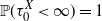 $\mathbb{P}(\tau_0^X < \infty) = 1$
when
 $\phi_1(\lambda_1) > 0$
for any
 $\lambda_1 > 0$
, and
 $\mathbb{P}(\tau_0^Y < \infty) = 1$
if
 $\phi_2(\lambda_2) > 0$
for any
 $\lambda_2 > 0$
.
Corollary 3.1. Assume that
 $b \ge 0$
,
 $R_1 \;:\!=\; \int_{\mathbb{N}^{-1}}\xi\,n({\mathrm{d}}\xi) < 0$
, and Condition 3.1 holds. Then we have
 $\mathbb{P}_{z_0}\{\tau_{0}<\infty\} = 1$
.


3.2. Exponential ergodicity in the
$L^1$
-Wasserstein distance

The coupling method is a powerful tool in the study of ergodicity of Markov processes. We refer the reader to [Reference Chen6, Reference Lindvall20] for systematic study on this topic.
We say a process
 $(Z_1(t),Z_2(t))_{t\geq0}$
is a coupling of
 $(Z(t))_{t\geq0}$
with transition semigroup
 $(P_t)_{t\geq0}$
if both
 $(Z_1(t))_{t\geq0}$
and
 $(Z_2(t))_{t\geq0}$
are Markov processes with transition semigroup
 $(P_t)_{t\geq0}$
(possibly with different initial distributions) and
 $Z_1(t+\tau) = Z_2(t+\tau)$
for every
 $t\geq0$
, where
 $\tau=\inf\{t\geq0\colon Z_1(t)=Z_2(t)\}$
. In this case,
 $(Z_1(t))_{t\geq0}$
and
 $(Z_2(t))_{t\geq0}$
are called the marginal processes of the coupling. Let A and
 $\tilde{A}$
be infinitesimal generators of
 $(Z(t))_{t\geq0}$
and
 $(Z_1(t),Z_2(t))_{t\geq0}$
, respectively. Then
 $\tilde{A}$
is called the coupling generator and satisfies the marginal property, i.e. for any
 $f,g\in{\mathcal{D}}(A)$
,
 \begin{equation} \tilde{A}u(z,\tilde{z})=Af(z)+Ag(\tilde{z})\end{equation}
with
 $u(z,\tilde{z})=f(z)+g(\tilde{z})$
.
A coupling
 $(Z_1(t),Z_2(t))_{t\geq0}$
is called successful if
 $\tau<\infty$
almost surely. A Markov process is said to have a coupling property if, for any initial distributions
 $\mu_1$
and
 $\mu_2$
, there exists a successful coupling with marginal processes starting from
 $\mu_1$
and
 $\mu_2$
, respectively. For any initial distribution
 $\mu$
, let
 $\mathbb{P}^\mu$
be the distribution of this process with initial distribution
 $\mu$
, and let
 $\mu P_t$
be the marginal distribution of
 $ \mathbb{P}^\mu$
. It is known [Reference Cranston and Greven8, Reference Lindvall20] that the coupling property of the process is equivalent to the statement
 \begin{equation*} \mbox{for any initial distributions}\ \mu_1,\mu_2,\ \lim_{t\rightarrow\infty}\|\mu_1P_t-\mu_2P_t\|_{\mathrm{var}}=0,\end{equation*}
where
 $\|\cdot\|_{\mathrm{var}}$
is the total variation norm in the sense of
 \begin{equation*} \|\mu-\nu\|_\mathrm{var} \;:\!=\; \sup\{|\mu(A)-\nu(A)|\colon A\ \text{is a Borel set}\}.\end{equation*}
The total variation norm is a special case of Wasserstein distances. By
 $\mathcal{P}(D)$
we denote the space of all Borel probability measures over D. Given
 $\mu,\nu\in\mathcal{P}(D)$
, a coupling H of
 $(\mu,\nu)$
is a Borel probability measure on
 $D\times D$
which has marginals
 $\mu$
and
 $\nu$
, respectively. We write
 $\mathcal{H}(\mu,\nu)$
for the collection of all such couplings. Let d be a metric on D such that (D, d) is a complete separable metric space, and define
 $$\mathcal{P}_d(D)\;:\!=\;\bigg\{\rho\in\mathcal{P}(D)\colon\displaystyle\int_Dd(z,0)\,\rho({\mathrm{d}}z)<\infty\bigg\}.$$
Then the Wasserstein distance on
 $\mathcal{P}_d(D)$
is defined by
 $$W_d(\mu,\nu) \;:\!=\; \inf\bigg\{\displaystyle\int_{D\times D}d(z,\tilde{z})\,H({\mathrm{d}}z,{\mathrm{d}}\tilde{z}) \colon H\in\mathcal{H}(\mu,\nu)\bigg\}.$$
Moreover, it can be shown that this infimum is attained; see, e.g., [Reference Villani33, Theorem 6.16]. More precisely, there exists
 $\tilde{H}\in{\mathcal{H}}(\mu,\nu)$
such that
 $W_d(\mu,\nu)=\int_{D\times D}d(z,\tilde{z})\,\tilde{H}({\mathrm{d}} z,{\mathrm{d}} \tilde{z})$
. By taking
 $d(z,\tilde{z})=\|z-\tilde{z}\|_1$
, we have
 $\mathcal{P}_d(D)\;:\!=\;\mathcal{P}_1(D)$
defined by
 \begin{equation*} \mathcal{P}_1(D)\;:\!=\;\bigg\{\rho\in\mathcal{P}(D)\colon\displaystyle\int_D\|z\|_1\,\rho({\mathrm{d}}z)<\infty\bigg\},\end{equation*}
where
 $\|\cdot\|_1$
is the
 $L^1$
norm on D. We say the corresponding Wasserstein distance
 $W_1$
is the
 $L^1$
-Wasserstein distance.
Definition 3.1. We say
 $(Z(t))_{t\geq0}$
on D or its transition semigroup
 $(P_t)_{t\geq0}$
is exponentially ergodic in the
 $L^1$
-Wasserstein distance with rate
 $\lambda_0>0$
if it possesses a unique stationary distribution
 $\mu$
and there is a non-negative function
 $\nu\mapsto C(\nu)$
on
 $\mathcal{P}(D)$
such that
 \begin{equation} W_1(\nu P_t,\mu) \leq C(\nu){\mathrm{e}}^{-\lambda_0 t}, \quad t\geq0,\,\nu\in\mathcal{P}(D). \end{equation}
Let
 $P_t(z,\cdot)$
be the transition probability kernel of the process with the initial value z. By standard arguments, (3.3) follows if
 \begin{equation} W_1(P_t(z,\cdot),P_t(\tilde{z},\cdot))\leq C_0(z,\tilde{z}){\mathrm{e}}^{-\lambda_0t},\quad t\geq0,\end{equation}
for a constant
 $C_0(z,\tilde{z})>0$
depending on z and
 $\tilde{z}$
; see, e.g., the proof of [Reference Friesen, Jin, Kremer and Rüdiger14, Theorem 3.5].
In the literature of the exponential ergodicity of branching processes, [Reference Chen and Li7, Reference Friesen, Jin, Kremer and Rüdiger14, Reference Li26, Reference Li and Ma27] obtained results by making full use of the branching property. If the property fails, it has been shown that coupling methods are very effective; see, e.g., [Reference Li, Li, Wang and Zhou21, Reference Li and Wang22]. In this subsection we mainly consider that the rate function
 $h(\cdot,\cdot)$
satisfies, for any
 $z=(x,y)\in D$
,
 $h(x,y)=r+x\ell(y)$
, with
 $r>0$
and
 $\ell(\cdot)$
being a non-negative function on
 $\mathbb{N}$
.
This subsection consists of two parts. First, we need to construct a coupling for the mixed-state branching process with interactions
 $(Z(t))_{t\geq0}=(X(t),Y(t))_{t\geq0}$
. Second, due to the comparison property of X, we construct a proper function
 $F_{\theta}(x,y,\tilde{x},\tilde{y})=F_{\theta}(x-\tilde{x},|y-\tilde{y}|)$
for any
 $z=(x,y),\tilde{z}=(\tilde{x},\tilde{z})\in D$
with
 $x\geq\tilde{x}$
satisfying two properties:
-
(i) the exponential contraction property: for any
$z=(x,y),\tilde{z}=(\tilde{x},\tilde{y})\in D$
with
$x\geq\tilde{x}$
, for some
$$ \tilde{A} F_{\theta}(x-\tilde{x},|y-\tilde{y}|)\leq-\lambda F_{\theta}(x-\tilde{x},|y-\tilde{y}|) $$
$\lambda>0$
, where
$\tilde{A}$
denotes the coupling generator;
-
(ii) control the
$L^1$
-Wasserstein distance in the sense that where
$$ F_{\theta}(x-\tilde{x},|y-\tilde{y}|)\asymp x-\tilde{x}+|y-\tilde{y}|, $$
$f\asymp g$
means that there is a constant
$C_1\geq1$
such that
$C_1^{-1}f(\cdot)\leq g(\cdot)\leq C_1f(\cdot)$
.



Then we can deduce (3.4) from (i) and (ii); see, e.g., the arguments in [Reference Luo and Wang29, Theorem 3.1, part (2)] or [Reference Li and Wang22, Lemma 4.3].
Recall that the generator A of
 $(Z(t))_{t\geq0}=(X(t),Y(t))_{t\geq0}$
is given by (2.1) for any
 $f\in \mathcal{D}(A)$
. To study the coupling and ergodicity of the process, we begin with the construction of a new coupling operator. We will combine coupling by reflection for the Brownian motion and synchronous coupling for Poisson random measures. Here, the coupling by reflection for Brownian motion means that we will take
 $(\!-B(t))_{t\geq0}$
(which is regarded as a reflection of
 $(B(t))_{t\geq0}$
) for the process
 $(X(t))_{t\geq0}$
before two marginal processes meet. To explain the meaning of synchronous coupling for Poisson random measures, we will use the viewpoint of the coupling operator. Set
 $z=(x,y)$
,
 $\tilde{z}=(\tilde{x},\tilde{y})\in D$
with
 $x\geq\tilde{x}$
. Recall that
 $\gamma(x,y)=yh(x,y)$
. The jump system corresponding to the synchronous coupling for the operator A is given by
 \begin{align*} (x,\tilde{x}) & \rightarrow \begin{cases} (x+\xi,\tilde{x}+\xi), & \tilde{x}\,m({\mathrm{d}}\xi), \\[5pt] (x+\xi,\tilde{x}), & (x - \tilde{x})\,m({\mathrm{d}}\xi), \end{cases} \\[5pt] (y,\tilde{y}) & \rightarrow \begin{cases} (y+\xi,\tilde{y}+\xi), & [\gamma(x,y)\wedge\gamma(\tilde{x},\tilde{y})]\,n({\mathrm{d}}\xi), \\[5pt] (y+\xi,\tilde{y}), & [\gamma(x,y)-\gamma(\tilde{x},\tilde{y})]^+\,n({\mathrm{d}}\xi), \\[5pt] (y,\tilde{y}+\xi), & [\gamma(x,y)-\gamma(\tilde{x},\tilde{y})]^-\,n({\mathrm{d}}\xi), \end{cases} \end{align*}
where
 $f^+$
(resp.
 $f^-$
) denotes the positive (resp. negative) part of function f. Similarly, we can define the jump system for the case of
 $x<\tilde{x}$
. We refer to [Reference Chen6] for the details of such a coupling, and other couplings for jump systems. We also refer to [Reference Li and Wang22, Remark 2.4] for similar discussions in the setting of nonlinear CB-processes. Let
 ${C^2}(D\times D)^+$
be the set of non-negative continuous functions
 $(x, y, \tilde{x}, \tilde{y})\mapsto F(x, y, \tilde{x}, \tilde{y})$
on
 $D\times D$
with continuous derivatives up to the second order of x and
 $\tilde{x}$
. With the idea above in mind, we then define, for any
 $F\in \mathcal{D}(\tilde{A})$
and
 $x\geq\tilde{x}$
,
 \begin{align} \tilde{A}F(x,y,\tilde{x},\tilde{y}) & = -bxF'_x-b\tilde{x}F'_{\tilde{x}} + cxF''_{xx} + c\tilde{x}F''_{\tilde{x}\tilde{x}} - 2c\sqrt{x\tilde{x}}F''_{x\tilde{x}} \cr & \quad + \tilde{x}\displaystyle\int_0^\infty[F(x+\xi,y,\tilde{x}+\xi,\tilde{y})-F(x,y,\tilde{x}, \tilde{y})-\xi(F'_x+F'_{\tilde{x}})]\,m({\mathrm{d}}\xi) \cr & \quad + (x-\tilde{x})\displaystyle\int_0^\infty[F(x+\xi,y,\tilde{x},\tilde{y})-F(x,y,\tilde{x},\tilde{y})-\xi F'_x]\, m({\mathrm{d}}\xi) \cr & \quad + [\gamma(x,y)\wedge\gamma(\tilde{x},\tilde{y})]\displaystyle\int_{\mathbb{N}^{-1}} [F(x,y+\xi,\tilde{x},\tilde{y}+\xi)-F(x,y,\tilde{x},\tilde{y})]\,n({\mathrm{d}}\xi) \cr & \quad + [\gamma(x,y)-\gamma(\tilde{x},\tilde{y})]^+\displaystyle\int_{\mathbb{N}^{-1}} [F(x,y+\xi,\tilde{x},\tilde{y})-F(x,y,\tilde{x},\tilde{y})]\,n({\mathrm{d}}\xi) \cr & \quad + [\gamma(x,y)-\gamma(\tilde{x},\tilde{y})]^-\displaystyle\int_{\mathbb{N}^{-1}} [F(x,y,\tilde{x},\tilde{y}+\xi)-F(x,y,\tilde{x},\tilde{y})]\,n({\mathrm{d}}\xi), \end{align}
where
 $\mathcal{D}(\tilde{A})$
denotes the linear space consisting of functions
 $f\in C^{2}(D\times D)^+$
such that the five integrals on the right-hand side of (3.5) are convergent and define continuous functions on
 $D\times D$
. Here and in what follows,
 $F'_x={\partial F(x,y,\tilde{x},\tilde{y})}/{\partial x}$
,
 $F''_{xx}={\partial^2 F(x,y,\tilde{x},\tilde{y})}/{\partial x^2}$
, and so on. Similarly, we can define
 $\tilde{A}F(x,y,\tilde{x},\tilde{y})$
for the case that
 $x<\tilde{x}$
. By (3.2), it is not hard to see that
 $\tilde{A}$
is indeed a coupling generator of A defined by (2.1).
Theorem 3.2. There exists a coupling
 $(Z(t),\tilde{Z}(t))_{t\geq0}=(X(t),Y(t),\tilde{X}(t),\tilde{Y}(t))_{t\geq0}$
whose generator is
 $\tilde{A}$
.
Proof. We consider the following SDE:

where
 \begin{equation*} B^*(t) = \begin{cases} -B(t), & t\leq T, \cr -2B(T)+B(t), & t>T \end{cases} \end{equation*}
and
 $T=\inf\{t>0\colon X(t)=\tilde{X}(t)\}$
. Clearly,
 $(B^*(t))_{t\geq0}$
is still a standard Brownian motion. By the results in Section 2, we can determine the unique strong solution
 $(Z(t),\tilde{Z}(t))_{t\geq0} \;:\!=\; (X(t),Y(t),\tilde{X}(t),\tilde{Y}(t))_{t\geq0}$
to (3.6). On the other hand, we can apply Itô’s formula to the SDE (3.6) to see that the infinitesimal generator of the process
 $(Z(t),\tilde{Z}(t))_{t\geq0}$
is indeed the coupling generator defined by (3.5).
Now, for any
 $\theta>0$
we define the function
 $F_{\theta}$
as
 $F_{\theta}(s,t)=s+\theta t$
,
 $s,t\geq0$
. It is easy to see that
 $F_{\theta}(s,t)\asymp s+t$
. For the main result in this subsection, we require the following assumptions.
Condition 3.2.
 $b > 0$
and
 $R_1\;:\!=\;\int_{\mathbb{N}^{-1}}\xi\,n({\mathrm{d}}\xi) < 0$
.
Condition 3.3.
For any
 $y\in\mathbb{N}_+$
,
 $y\mapsto \ell(y)y$
is non-decreasing and bounded in the sense of
 $R_2\;:\!=\;\sup_{y\in\mathbb{N}_+}\ell(y)y<\infty$
.
Remark 3.2.
X is a subcritical CB-process under the assumption of
 $b>0$
; see, e.g., [Reference Li25, Reference Li26]. No specific restrictions are placed on the Lévy noise in this paper, which is reasonable given our primary focus on exponential ergodicity in the
 $L^1$
-Wasserstein distance. However, when considering the exponential ergodicity in the total variation distance for CB-processes, some additional assumptions on the Lévy noise is required; see, e.g., [Reference Friesen, Jin, Kremer and Rüdiger14, Reference Li and Ma27]. In the case of state-dependent branching, even in the
 $L^1$
-Wasserstein distance, some restrictions on the Lévy noise is necessary; see [Reference Li and Wang22]. Furthermore, we note that in other distance spaces
 $W_d$
, or for state-dependent cases, more complex functions are required.
Remark 3.3. Under the assumption of
 $R_1 < 0$
in Condition 3.2, the first moment of the offspring distribution of each individual is strictly less than 1, i.e.
 $\sum_{j}jp_j<1$
. In this case, the continuous-time Markov branching process Y is subcritical when h is a positive constant; see, e.g., [Reference Athreya and Ney2, p. 112].
Remark 3.4. Condition 3.3 holds when
 $\ell(\cdot)\equiv0$
. In this case,
 $(Y(t))_{t\geq0}$
is a standard continuous-time branching process with branching rate
 $r>0$
and offspring
 $(p_\xi,\xi\in\mathbb{N})$
. Condition 3.3 also holds when
 $\ell(y)={1}/({y+1})$
. In this case, as the number of cells increases, the rate of cell division gets slower.
We now present the main result.
Theorem 3.3 Suppose that Conditions 3.2 and 3.3 are satisfied. Then there are constants
 $\lambda_0>0$
such that, for any
 $(x,y),(\tilde{x},\tilde{y})\in D$
, (3.4) holds.
Proof. It suffices to consider
 $x\geq\tilde{x}$
. Considering
 $F_\theta(x,\tilde{x},y,\tilde{y})\;:\!=\;F_{\theta}(x-\tilde{x},|y-\tilde{y}|)$
, (3.5), and Taylor’s formula, we have
 \begin{align*} & \tilde{A}F_{\theta}(x-\tilde{x},|y-\tilde{y}|) \cr & \leq - b(x-\tilde{x}) + \theta[\gamma(x,y)-\gamma(\tilde{x},\tilde{y})]^+ \displaystyle\int_{\mathbb{N}^{-1}}[|y-\tilde{y}+\xi|-|y-\tilde{y}|]\,n({\mathrm{d}}\xi) \cr & \quad + \theta[\gamma(x,y)-\gamma(\tilde{x},\tilde{y})]^- \displaystyle\int_{\mathbb{N}^{-1}}[|y-\tilde{y}-\xi|-|y-\tilde{y}|]\,n({\mathrm{d}}\xi) \cr & \leq - b(x-\tilde{x}) + \theta[\gamma(x,y)-\gamma(\tilde{x},\tilde{y})]^+\textbf{1}_{\{y>\tilde{y}\}} \displaystyle\int_{\mathbb{N}^{-1}}\xi\,n({\mathrm{d}}\xi) \cr & \quad + \theta[\gamma(x,y)-\gamma(\tilde{x},\tilde{y})]^+\textbf{1}_{\{y\leq\tilde{y}\}} \displaystyle\int_{\mathbb{N}^{-1}}|\xi|\,n({\mathrm{d}}\xi) + \theta[\gamma(x,y)-\gamma(\tilde{x},\tilde{y})]^- \textbf{1}_{\{y>\tilde{y}\}}\displaystyle\int_{\mathbb{N}^{-1}}|\xi|\,n({\mathrm{d}}\xi) \cr & \quad + \theta[\gamma(x,y)-\gamma(\tilde{x},\tilde{y})]^-\textbf{1}_{\{y\leq\tilde{y}\}} \displaystyle\int_{\mathbb{N}^{-1}}\xi\,n({\mathrm{d}}\xi). \end{align*}
Since
 $\gamma(x,y)=ry+x\ell(y)y$
, we arrive at
 \begin{align*} \tilde{A}F_{\theta}(x-\tilde{x},|y-\tilde{y}|) & \leq -b(x-\tilde{x}) - \theta n(\{-1\})(\gamma(x,y)-\gamma(\tilde{x},\tilde{y})) \frac{y-\tilde{y}}{|y-\tilde{y}|} \cr & \quad + \theta\displaystyle\int_{\mathbb{N}}\xi\,n({\mathrm{d}}\xi)|\gamma(x,y)-\gamma(\tilde{x},\tilde{y})| \cr & = -b(x-\tilde{x}) - \theta n(\{-1\})(ry-r\tilde{y}+x\ell(y)y-\tilde{x}\ell(\tilde{y})\tilde{y}) \frac{y-\tilde{y}}{|y-\tilde{y}|} \cr & \quad + \theta\displaystyle\int_{\mathbb{N}}\xi\,n({\mathrm{d}}\xi)|ry - r\tilde{y} + x\ell(y)y - \tilde{x}\ell(\tilde{y})\tilde{y}|. \end{align*}
Notice that
 $\int_{\mathbb{N}^{-1}}|\xi|\,n({\mathrm{d}}\xi)\in(0,\infty)$
by
 $R_1 \in (\!-\infty, 0)$
of Condition 3.2. By Condition 3.3, we have
 \begin{align*} & \tilde{A}F_{\theta}(x-\tilde{x},|y-\tilde{y}|) \\[5pt] & \leq -b(x-\tilde{x}) - \theta n(\{-1\})\bigg(r|y-\tilde{y}| + (x-\tilde{x})\ell(y)y\frac{y-\tilde{y}}{|y-\tilde{y}|} + \tilde{x}(\ell(y)y - \ell(\tilde{y})\tilde{y})\frac{y-\tilde{y}}{|y-\tilde{y}|}\bigg) \cr & \quad + \theta\displaystyle\int_{\mathbb{N}}\xi\,n({\mathrm{d}}\xi)(r|y-\tilde{y}| + (x-\tilde{x})\ell(y)y + \tilde{x}|\ell(y)y-\ell(\tilde{y})\tilde{y}|) \cr & \leq - \bigg(b - \theta\displaystyle\int_{\mathbb{N}^{-1}}|\xi|\,n({\mathrm{d}}\xi)\ell(y)y\bigg)(x-\tilde{x}) + \theta rR_1|y-\tilde{y}| + \tilde{x}\theta R_1|\ell(y)y - \ell(\tilde{y})\tilde{y}| \cr & \leq - \bigg(b - \theta R_2\displaystyle\int_{\mathbb{N}^{-1}}|\xi|\,n({\mathrm{d}}\xi)\bigg)(x-\tilde{x}) + \theta r R_1|y-\tilde{y}| \cr & \leq - \lambda_1F_{\theta}(x-\tilde{x},|y-\tilde{y}|) \end{align*}
for some
 $\lambda_1>0$
by setting
 $$\theta\;:\!=\;\theta_1=\frac{b}{2R_2\displaystyle\int_{\mathbb{N}^{-1}}|\xi|\,n({\mathrm{d}}\xi)}.$$
Following similar arguments to step 2 of the proof of [Reference Luo and Wang29, Theorem 3.1], we obtain the desired result.
Acknowledgements
We are grateful to the editors and two referees for their careful reading of the paper and their helpful comments.
Funding information
The research of S. Chen was supported in part by National Key R&D Program of China (No. 2022YFA1006003), NSFC grant (No. 12401167), NSF-Fujian grant (No. 2024J08050) and the Education and Scientific Research Project for Young and Middle-aged Teachers in Fujian Province of China (No. JAT231015). The research of L. Ji was supported in part by NSFC grant (Nos. 12301167 and 12271029), Guangdong Basic and Applied Basic Research Foundation (No. 2022A1515110986) and Shenzhen National Science Foundation (No. 20231128093607001). The research of J. Xiong was supported in part by National Key R&D Program of China grant (No. 2022YFA1006102) and NSFC grant (No. 12471418).
Competing interests
There were no competing interests to declare which arose during the preparation or publication process of this article.


