The correspondence between public preferences and public policy is a critical rationale for representative democratic government. This view has been put forward in the theoretical literature on democracy and representation (e.g., Dahl 1971; Pitkin 1967; Birch 1971) and in “functional” theories of democratic politics (Easton 1965; Deutsch 1963), both of which emphasize the importance of popular control of policymaking institutions. Political science research also shows a good amount of correspondence between opinion and policy, though to varying degrees, across a range of policy domains and political institutions in the U.S. and elsewhere.1
The literature is vast. Critical early work focusing on the national level in the U.S. includes Miller and Stokes (1963); Weissberg (1976); and Monroe (1979); for more recent research, see Stimson, MacKuen, and Erikson (1995). Important work at the state level includes Erikson, Wright, and McIver (1995). For research on other countries, see, e.g., Petry (1999); Soroka and Wlezien (2004; 2005); Hobolt and Klemmensen (2005); Brooks and Manza (2006). For useful reviews of the literature, see Burstein (1998) and Weakliem (2003).
Alongside this work there is an increasing focus on the equality of representation—specifically, “procedural equality,” where “the political preferences expressed by each citizen receive equal weight in the decision-making process” (Beitz 1990). That this version of equality is critical to most modern democratic thinking requires little discussion here.2
Bartels' (2006) note on inequality in American democracy provides a clear statement on the commonly-held belief that equality is central to responsive and representative government.
We address this issue by taking a step backward rather than forward. The new literature has nicely captured differences in responsiveness across income brackets, at least for certain policies or else in a broad “global” way across policies. We nevertheless still have only a partial understanding of the extent of the difference in public policy preferences across income brackets, or other sub-aggregates such as education or party identification. This is important, as differential representation requires, at a minimum, differences in public preferences. Establishing where these differences exist is a critical—and, we believe, largely overlooked—step in evaluating the magnitude of inequality in representation.
This paper explores differences in public preferences for policy across sub-aggregates based on income, education, and party identification in the U.S. We focus primarily on a set of spending domains of recurring political importance, where governments have tended to be quite responsive, both in the U.S. and elsewhere (e.g., Soroka and Wlezien 2004, 2005; Wlezien 1996, 2004). Our results indicate that income really only matters in isolated cases, specifically, welfare spending preferences. In the other domains, differences in preferences across income brackets are in fact small and insignificant. (Differences are much greater across education levels and, especially, party identification.) These results have important implications for the study of representation. Put simply, they suggest that the scope for inequality in policy representation, by income groups at least, is rather limited. Before examining the data, however, we offer a general model of political representation across different population sub-aggregates.
Inequality in Political Representation
A central tenet of representative democratic governance is that policy will be a function of preferences. That is,

where OpinionAll is some summary of the policy preferences of all citizens within the unit—country, state, or locality—of interest.3
Note that this representation of opinion can occur in two ways: indirectly, through elections, or directly, where sitting politicians literally respond to what the public wants. These two ways to representation are in a broad sense related—that is, the first way implies the second, at least assuming incumbent politicians are interested in remaining in office. Elected officials are expected to respond to public preferences, even between elections, because of the threat of electoral sanction. Of course, it may also be that politicians want to represent public preferences for other reasons.
Also, consider the difference between using the mean or the median. Changes in a single preference at one end of the distribution will not affect the median but will affect the mean. Representation of the mean preference thus has a certain kind of built-in inequality—depending on their place in the overall distribution, marginal changes in each individual preference will affect the summary of aggregate preferences to a varying degree. Representation of the median preference implies a different kind of inequality—in this case, it is marginal changes in the middle of the distribution that matter. Note that Dahl's (1956) discussion of “Equality, Diversity and Intensity” reflects similar concerns about how to summarize preferences in an equitable way.
The inequality we are interested in here is one based on politically relevant sub-aggregates, specifically, income, education, and party identification. That is, we are concerned with the possibility that representation will be driven more by the preferences of wealthy citizens, for instance, than by the preferences of poor citizens. Following from Equation 1, a model capturing inequality in representation can be portrayed as follows,

where the preferences of high-, medium- and low-income respondents are entered into the model separately. The division by income terciles is of course just one possibility, and this model can just as easily capture differences across other breakdowns of income, or other variables such as education, partisan identification, race, and gender. Regardless, evidence of inequality is captured in Equation 2 by the potentially differing effects of each category of opinion. What we wish to emphasize here is that the potential for differing effects of each category of opinion is dependent on there being significant differences across categories.
Variations of Equation 2 have been the focus of recent work on policy inequality. Bartels (2005) relates average scores on the National Election Study (NES) ideology question, by income tercile, to U.S. Senators' roll-call votes.5
To be precise, Bartels looks at Senators' W-NOMINATE ideological scores, as determined by their roll-call votes, as well as a number of specific roll-call votes.
Jacobs and Page (2005) explore a different though related theme. They do not look specifically at the effects of public preferences across income categories, but examine the varying associations between U.S. foreign policy officials and those of business leaders, experts, labour, or the general public. More so than others, however, they directly examine opinion change, and find that one-period change in policy support found amongst U.S. foreign policy officials most closely matches one-period change in the preferences of business leaders and experts. This provides further—albeit more indirect—evidence of a representational bias toward upper-income citizens.6
Note that this analysis of one-period change is just one of Jacobs and Page's analyses. They also examine opinion-policy relationships in levels, first excluding and then including one-period-lagged opinion and policy.
These results clearly are provocative and important. Each of the studies indicates a substantial bias in the representation connection. We seek to add to this literature here, albeit in a different way. We do not focus on models of opinion and policy outcomes, but instead engage in a simple diagnostic exercise. We take measures of public preferences for policy, directly comparable across policy domains and over time, and examine the degree to which preferences vary across three different politically salient sets of sub-aggregates—income, education, party identification. The potential for unequal representation is first and foremost dependent on the differences (or similarities) we find in the sections that follow.
Public Preferences for Spending
Our focus is on measures of public preferences for government spending in eight major spending domains. The data are based on the following question, included regularly in the U.S. General Social Survey (GSS) surveys (and elsewhere):
We are faced with many problems in this country, none of which can be solved easily or inexpensively. I'm going to name some of these problems, and for each one I'd like you to tell me whether you think we're spending too much money on it, too little money, or about the right amount. Do you think the government is spending too much, too little or about the right amount on [healthcare]?
Notice that the question asks about preferences for government spending in general, not at particular levels of government, e.g., the nation, the state, the locality. It also asks about people's relative preferences—their preference for policy change—not their absolute preferences. Respondents are asked consistently about spending in other categories besides healthcare in the GSS in almost every year from 1973 to 1994, and then in alternate years until 2004, 24 years in total. Using responses to these questions, where question wording is identical over time and across domains, allows us to assess whether and to what extent differences are truly systematic and not unique to particular times and domains. We focus specifically on the eight areas that have been asked on a recurring basis: cities, crime, defense, education, the environment, foreign aid, health, and welfare.
From the responses, we generate a summary measure of net support for each domain across years. The measure is the percentage of people who think we are spending “too much” minus the percentage of people who think we are spending “too little” in each domain. The measure thus captures both the direction and magnitude of the preference for policy change. For our work here, we calculate net support separately for sub-aggregates of income, education, and party identification. For income, we separate respondents into income terciles, based on the income levels reported in the GSS.7
Using terciles from the GSS has the advantage of keeping our three categories equal in size—that is, the number of respondents in each category is the same, and no one category is more (or less) susceptible to measurement error. (For income categories, and others, the total sample size is just over 1,100 on average. Approximately 5% of respondents do not answer the income question, leaving an average N of about 1,050, or 350 in each income category.) Given that the income distribution reported to GSS always is lower than what we see in Census data, we also calculated using terciles from the U.S. Census bureau. This makes virtually no difference to any of the results—specifically, using the Census distribution slightly expands the range of differences. To determine preferences by income tercile, we begin with preferences aggregated by whatever income response categories exist in the individual-level survey file. We then collapse these into income terciles. When survey response categories overlap the divide between two income terciles, the respondents in this category are assigned the mean score (in the category) and allocated to the two income terciles proportionally, based on where the tercile division lies.
There are some predictable exceptions. The sizes of the education groups do change over time, for instance, and in predictable ways: the percentage of people not finishing high school declines and the percentage of people who have some college education increases.
Independents here include both the “pure” independents and those who “lean” toward one of the parties.
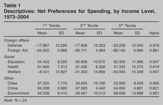
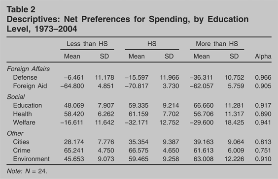
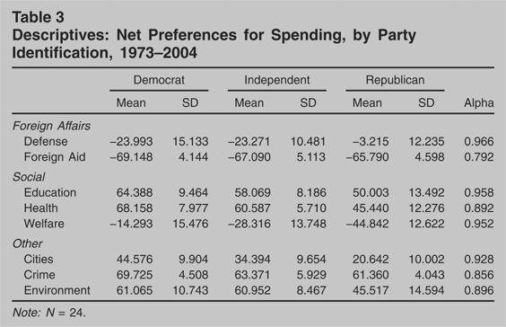
Tables 1, 2, and 3 provide basic descriptive statistics for the different sub-aggregates—income, education, and party identification. Columns 1 through 6 show the mean and standard deviation for each of the eight preferences series. The last column shows Cronbach's alpha, a standard summary measure of bivariate correlations between the three sub-aggregate series. The alpha gives us a sense for how closely each set of three series moves together over time, i.e., the degree to which the differences or similarities across groups are consistent.10
Note, however, that alphas can be taken to overstate the parallelism between series. For instance, an average bivariate correlation of .5 produces an alpha of .75.
Descriptives: Net Preferences for Spending, by Income Level, 1973–2004

Descriptives: Net Preferences for Spending, by Education Level, 1973–2004

Descriptives: Net Preferences for Spending, by Party Identification, 1973–2004


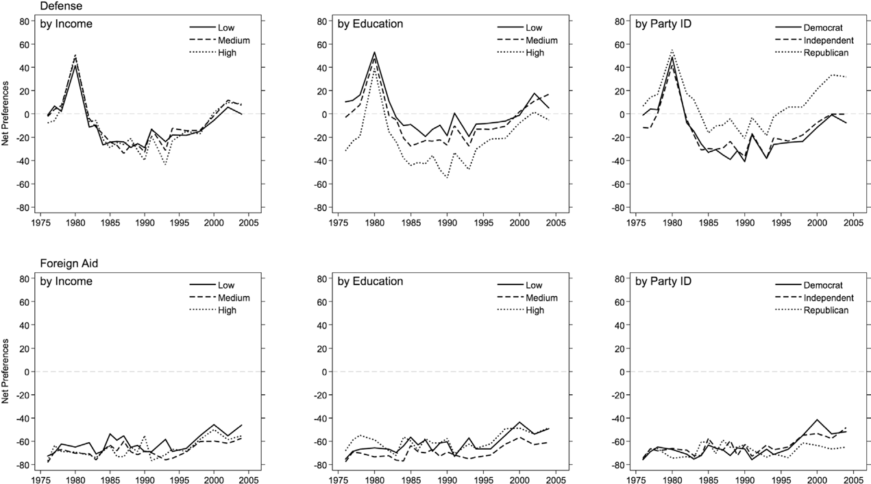
Net Preferences for Spending, Foreign Affairs Domains

Net Preferences for Spending, Social Policy Domains

Net Preferences for Spending, Other Policy Domains
Let us first consider the results for income categories in Table 1. Here we can see relatively little heterogeneity in spending preferences across income levels in most domains, in all domains but welfare spending, that is. Compare the means by income tercile. The difference in means for the non-welfare spending domains is less than four points on average, only three points when comparing people with high and low incomes. None of these differences are even close to statistically significant.
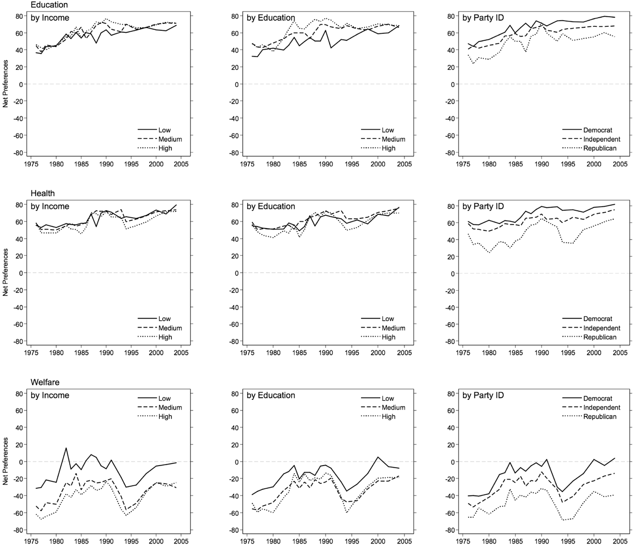
Things are different for the welfare spending domain. Here we see sizable differences. The means differ by over 30 points, five times what we observed for the other seven domains, on average. Notice also that the differences across income levels are not symmetrical. The mean preference for people with middling incomes is much more like the mean for people with upper incomes. From the point of view of representation, this is of obvious importance. First, if politicians represent the median voter, policy may be very different from what the poor would prefer. Second, if politicians represent the upper-income tercile, policy will tend to be fairly similar to what the median voter would want. In the other domains, of course, there is little basis for differential representation, as preferences are essentially the same regardless of income level.11
To the extent one takes the 0-point seriously, note that the “direction” of public preferences rarely differs. For the eight domains taken together, preferences among the low- and high-income terciles are on different sides of 0—where one group favors more spending and the other less—only 5% of the time (29% of the time for welfare). The percentage drops to 4% for the low- and middle-income terciles and to 1% for the middle- and high-income terciles. Of course, it is not clear what the 0-point represents—we do know that the language used in the survey question can make a big difference, e.g., using “assistance to the poor” instead of “welfare” produces fundamentally different results (see, e.g., Weaver, Shapiro, and Jacobs 1995).
This does not mean that there is little heterogeneity in preferences. Table 2 shows that dividing respondents by education generates much larger differences on average. The means differ across sub-aggregates by about 14 points on average for the non-welfare domains—double what we saw for income. The preference gap between those with at least some college education and those who haven't completed high school is as much as four times the gap for upper- and lower-income terciles. The education gap is greatest for defense spending. It also is fairly large for welfare spending, but much narrower than we saw across income levels, implying that education levels are less reflective of differences in welfare self-interest.
The gaps in preferences typically are greater still across categories of party identification (see Table 3). This comes as little surprise, given the well-known link between party identification and issue preferences in many domains.
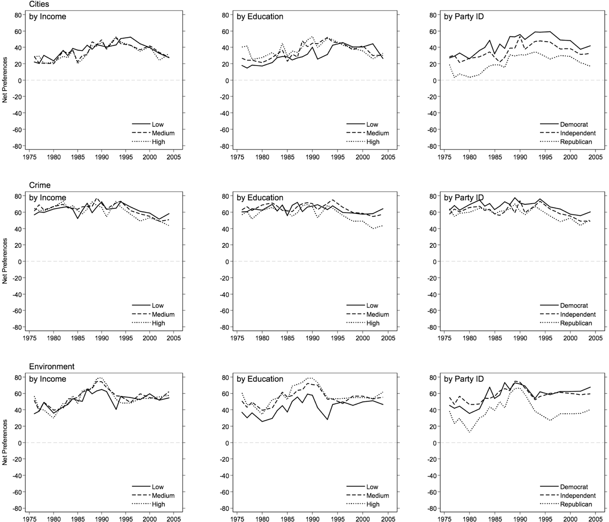
These general patterns across categories of income, education, and party identification are readily apparent in Figures 1, 2, and 3. With the exception of welfare spending, it is difficult to distinguish the preference series across income levels, shown in the first columns of the figures. The differences tend to widen when we turn to education in the second columns and then widen further for political parties, as can be seen in the third columns. In the figures it also is clear that preferences track each other over time. This is true regardless of differences in levels. In effect, there is substantial parallelism in preference change across segments of the population, as Page and Shapiro (1992) documented.12
The parallelism is not perfect, however. The alphas in Tables 1, 2, and 3 indicate that the correlations vary across domains, being most pronounced for defense, welfare, and education. In the tables we also observe that the preferences for some groups fluctuate more than others, e.g., the variance in preferences increases as income and, especially, education increases. Finally, there is some evidence of party polarization over time, at least in certain domains.
An ANOVA for welfare spending preferences across party identification and time indicates that the year variable accounts for 46% of total variance and party 49%. This is an important result, for it reveals that even where party matters most—on welfare—the common temporal movement matters just as much.
Public Preferences for Taxes
Why do our data show such small differences in policy preferences across income terciles? One possibility is that preferences tend to be more clearly different in policy domains where self-interest is paramount. Lower-income preferences are most clearly different for welfare spending, after all, where self-interest is pretty clear; the same may not be true of the other spending domains examined here. Gilens (2004) suggests a similar pattern. The non-spending domains in which self-interest is relevant also appear to show differences, particularly taxes. Thankfully, we do have data on tax preferences over time, and can assess systematic differences. In most years the GSS asks respondents about the amount of income tax they pay: “Do you consider the amount of federal income tax which you have to pay as too high, about right, or too low?”
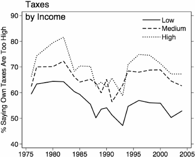
Not surprisingly, few people say “too low”—approximately 1%. Yet not everyone says “too high,” overall about 64%, and the proportion does differ some across income levels, as can be seen in Figure 4. On average, about 69% of people in the upper-income tercile think their taxes are too high as compared with 56% of those in the lower-income tercile. For middle-income people, the number is 66%, revealing a similar asymmetry to what we saw on welfare spending. Indeed, Figure 4 shows results quite similar to those for welfare spending: limited but significant cross-sectional differences between the preferences for lower-income respondents and the rest of the distribution, and parallelism over time.14
Changes in tax preferences appear less uniform across income levels than what we observed for spending (though note that the alpha is still a healthy .885), and in some years there is little difference at all across all three income groupings. This is quite understandable, as tax rates have changed in non-uniform ways over time, increasing for some groups—especially high-income citizens—in some periods and decreasing in other periods. Overall government spending, meanwhile, is the same for all individuals at each point in time.

Tax Preferences by Income Level
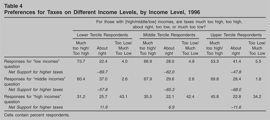
It may be that differences are more evident in individuals' preferences about the tax burdens of different income groups. In 1996, The GSS asked three related questions about the taxes for people with high incomes, middle incomes, and low incomes—specifically, “for those with high [middle/low] incomes, are taxes much too high, too high, about right, too low, or much too low?”15
The GSS also asked the question in 1987 though the differences across income categories in that year were comparatively small, about one-third of what we see in 1996. In 1987 and 2000 the GSS asked about whether “people with high incomes should pay a larger share of their income in taxes than those with low incomes, the same share, or a smaller share,” and the differences across income categories are smaller still.
Preferences for Taxes on Different Income Levels, by Income Level, 1996

The differences between income groups are most pronounced with regard to taxes on low- and high-income people. For instance, whereas 74% of the lower-income tercile think taxes on those with low incomes are too high, only 53% of high-income people hold the same opinion. Likewise, whereas 31% of the lower-income tercile think taxes on those with high incomes are too high, 46% of high-income citizens think this is true.
For purposes of comparison with the analysis of spending preferences, consider the implied “net support” for more taxes—the percentage saying taxes are too low minus the percentage saying taxes are too high. Not surprisingly, net support for more taxes on those with low incomes is well below zero across the three income terciles, indicating strong support for lower taxes. There is some difference in support across terciles, however, with the lower-income tercile being about 22% more supportive of lower taxes than the upper-income tercile. The middle-income tercile is in between. There is a similar gap in net support for taxes on those with high incomes. Here the lower-income tercile actually thinks taxes are too low on balance and the upper-income tercile thinks they are too high. The gap in scores is 23%, virtually identical to what we saw for taxing those with low incomes. Although these differences are real, they are not as striking as we might expect—about two-thirds of what we observed on welfare spending—and the difference in opinions about taxes on those with middle incomes is much lower, more like what we observed in the various other non-welfare spending domains. The differences are even less pronounced in other years (see note 15).
Discussion: On the Limits to Inequality
Recent research finds that U.S. policy is most responsive to the preferences of wealthier citizens. Examining the generalizability of these findings has been the focus of the current paper. We have done so by taking a step backwards, that is, by assessing the extent to which there are differences in policy preferences across income levels to begin with. The existence of difference obviously is a necessary condition for differential representation: If preferences are the same, it will not—empirically speaking—matter to whom policymakers respond.
The preceding results suggest that, in the range of recurring domains on which government spends money, income-related differences are limited. Welfare spending is the one striking exception; in other spending domains, there are no real differences across income levels. Even on welfare spending, the differences are asymmetric, between the poor on the one hand and the rest of the income distribution on the other, where it is difficult to distinguish middle- and high-income preferences. Much the same is true for taxes, though here the differences are less pronounced.
It may be that modest differences in preference make a big difference for policy. We can estimate the effect of opinion differences by taking advantage of previous analysis of opinion representation (Wlezien 2004) and “thermostatic” policy feedback (Wlezien 1995) in the U.S. That is, we can assume policymakers represent high-income preferences, and simulate the net effect on spending of using middle-income preferences in their place.16
The approach estimates how much spending is necessary to drive preferences down to the level we observe for high-income respondents. The estimate actually is a liberal one, as it presumes that the preference equilibrium would remain unchanged, i.e., not increase.
These results may come as a surprise. Perhaps the rather small differences across income brackets are a product of measurement issues. It may be that income groupings do not neatly tap real differences in self-interest—the lower-income tercile includes retirees and many new entrants to the work force, for example, and explicit indicators of “life chances,” or class, may work better.17
It is worth noting that the measures of net support will not fully capture real differences when most people's preferences are far from the 0-point. When most respondents want “more” spending, for instance, the measures will not pick up differences that are evident only within the “more” category, that is, when differences in the “less” category are relatively small. More nuanced measurement of relative preferences thus could reveal more inter-group difference relating not only to income but also education and party identification and other variables.
There are other possible explanations for the relative lack of difference across income groups. Perhaps there simply is not much basis for difference across income levels in many policy domains. It may be that self-interest does not differ very much. Or, there may be a real basis for difference, but people do not see their self-interest, i.e., low-income people may be misinformed about policy and how it affects their circumstances and others'.18
Consider Althaus' (2003) extensive investigation of information effects on policy preferences.
Of course, to the extent underlying preferences are hidden from us, they are hidden from politicians as well. There thus is only a limited basis for inequality in representation across income groups—regardless of whose preferences policymakers follow, differences across income groups are often rather small, and policy will end up in essentially the same place. This is not to dispute results showing that policymakers mostly follow the preferences of the rich (Gilens 2005; Bartels 2005). Indeed, we take that research to imply that policy would represent the median voter only because the preferences of people with middling incomes are much like the preferences of those with high incomes. From this perspective, representation of the middle would be indirect. Given that there are differences in preferences across income levels in some important policy domains and that new differences can emerge, unequal responsiveness is of obvious importance.
There are other aspects of inequality, however. One is education, and here we see much bigger gaps across levels. It may be that these differences matter for policy, e.g., that policy tends to represent the preferences of the better educated. There may be inequality in representation across other sub-aggregates as well, including race and ethnicity and gender. Griffin and Newman (2005) find that voters are better represented than non-voters, and this may underpin any differential representation that we observe across groups. Partisanship may also matter. If representatives focus on co-partisans—those citizens most likely to re-elect them (see Fenno 1978; also Hill and Hurley 2003)—partisan groups should receive unequal representation, albeit varying over time with the party control of government. This time-varying inequality in representation may matter quite a lot given the large differences in preferences by party identification surveyed above.19
It would also help explain striking shifts in policy when the partisan control of government changes.
There clearly are many different groups across which representation may vary. The resulting pattern ultimately may turn out to be quite complex, reflecting the salience that different groups attach to different issues, for example (see Hutchings 2003). This is an empirical question, of course. Whether and to what extent groups actually are represented equally is certain to occupy scholarly attention for some time, both in the U.S. and abroad. In the meantime, we must accept that income alone does not provide a very substantial basis for unequal outputs in most recurrent policy domains in the U.S.
Author Bios
Stuart N. Soroka is associate professor and William Dawson Scholar in the department of political science at McGill University. He is director of the Canadian Opinion Research Archive at Queen's University at Kingston. His work has focused on relationships between media, public opinion, and policy; recent research has appeared in the Journal of Politics and, with Wlezien, the British Journal of Political Science.
Christopher Wlezien is professor of political science and faculty affiliate in the Institute for Public Affairs at Temple University. He has published widely in the areas of elections, public opinion, and public policy, and recently co-edited Britain Votes (Oxford University Press) and The Future of Election Studies (Elsevier). He is coeditor of the international Journal of Elections, Public Opinion and Parties.