1 Introduction
Planets and stars generate and sustain their magnetic fields via the so-called hydromagnetic dynamo process (Elsasser Reference Elsasser1956), whereby the kinetic energy of fluid motion is converted into electromagnetic energy. Most natural dynamos are thought to be powered by buoyancy-driven convection resulting from thermal and/or compositional heterogeneities. The dynamics of natural dynamos is controlled and characterized by several non-dimensional parameters. Assuming the simplest case of an incompressible (i.e. Boussinesq) fluid layer of depth
 $H$
driven solely by the thermal heterogeneities, the strength of the buoyancy force is quantified by the Rayleigh number
 $Ra$
,
 $$\begin{eqnarray}Ra=\frac{g\unicode[STIX]{x1D6FE}\unicode[STIX]{x0394}\unicode[STIX]{x1D6E9}H^{3}}{\unicode[STIX]{x1D708}\unicode[STIX]{x1D705}},\end{eqnarray}$$
where
 $\unicode[STIX]{x1D6FE}$
is the thermal expansion coefficient,
 $g$
is the magnitude of the gravitational acceleration (assumed to be constant) and
 $\unicode[STIX]{x0394}\unicode[STIX]{x1D6E9}$
represents the temperature difference across the fluid layer. The viscosity and thermal diffusivity of the fluid are denoted by
 $\unicode[STIX]{x1D708}$
and
 $\unicode[STIX]{x1D705}$
, respectively, and their ratio defines the thermal Prandtl number
 $$\begin{eqnarray}Pr=\frac{\unicode[STIX]{x1D708}}{\unicode[STIX]{x1D705}}.\end{eqnarray}$$
All convectively driven planetary and stellar dynamos are estimated, or assumed, to be in the high Rayleigh number convective turbulence regime. For instance, values of
 $Ra>10^{20}$
characterize both the Earth’s liquid outer core and the solar convection zone (Ossendrijver Reference Ossendrijver2003; Schubert & Soderlund Reference Schubert and Soderlund2011).
The system rotation vector
 $\unicode[STIX]{x1D734}$
and the helical fluid motions it induces are thought to play an important role in the generation of large-scale magnetic fields (Parker Reference Parker1955). The dynamical influence of rotation on fluid motion is controlled by the Rossby and Ekman numbers, defined by
 $$\begin{eqnarray}Ro=\frac{U}{2\unicode[STIX]{x1D6FA}H},\quad E=\frac{\unicode[STIX]{x1D708}}{2\unicode[STIX]{x1D6FA}H^{2}},\end{eqnarray}$$
respectively measuring the strength of inertial forces relative to the Coriolis force, and viscous forces relative to the Coriolis force. Here
 $U$
is a characteristic flow speed and
 $\unicode[STIX]{x1D6FA}=|\unicode[STIX]{x1D734}|$
. Systems in which
 $(E,Ro)\ll 1$
are said to be rapidly rotating. For both the Earth’s liquid iron outer core and the Sun’s outer convective layer, the Ekman number is small with
 $E<10^{-14}$
. Moreover, the Rossby number based on observationally inferred speed and length scales for the core is
 $Ro\approx 10^{-6}$
(Finlay & Amit Reference Finlay and Amit2011). These values indicate that rotation strongly constrains fluid motions in the core. Estimating
 $Ro$
in the solar convection zone continues to be an important goal of stellar physics research, with recent helioseismic studies inferring values of
 $Ro\approx 0.1$
near the top of the convection zone (Hanosage, Duvall & Sreenivasan Reference Hanosage, Duvall and Sreenivasan2012; Greer et al.
Reference Greer, Hindman, Featherstone and Toomre2015).
The fluid properties of natural dynamos are known to have a significant effect on the convective motions (Jones Reference Jones2011). The thermal Prandtl number
 $Pr$
is less than unity in both planets and stars. Liquid metals such as in the Earth’s core are typically characterized by
 $Pr\approx 10^{-2}$
(Pozzo et al.
Reference Pozzo, Davies, Gubbins and Alfé2013) and stellar plasmas have extremely small values of
 $Pr\approx 10^{-7}$
(Ossendrijver Reference Ossendrijver2003). Laboratory experiments show that low
 $Pr$
convection is strongly inertial, thus allowing for the presence of turbulent motions at significantly lower Rayleigh numbers than required to achieve turbulence in
 $Pr\approx 1$
fluids (King & Aurnou Reference King and Aurnou2013; Aurnou et al.
Reference Aurnou, Calkins, Cheng, Julien, King, Nieves, Soderlund and Stellmach2015). The magnetic Prandtl number, defined as
 $$\begin{eqnarray}Pm=\unicode[STIX]{x1D708}/\unicode[STIX]{x1D702},\end{eqnarray}$$
where
 $\unicode[STIX]{x1D702}$
is the magnetic diffusivity, ranges from
 $Pm\approx 10^{-3}$
in the outer regions of the Sun, down to
 $Pm\approx 10^{-6}$
in the interiors of stars and planets.
Modelling natural dynamos is difficult due to the broad range of scales that characterize these systems and the concomitant numerical stiffness of the governing equations. Moreover, these challenges are compounded by the fact that rotation often leads to flow anisotropy (Chandrasekhar Reference Chandrasekhar1961). Despite these hindrances, direct numerical simulation (DNS) investigations continue to be the most widely employed method for dynamo studies (e.g. Jones Reference Jones2011; Tobias, Cattaneo & Boldyrev Reference Tobias, Cattaneo and Boldyrev2011). However, these studies are limited to relatively modest parameter values owing to computational restrictions; the recent study of Schaeffer et al. (Reference Schaeffer, Jault, Nataf and Fournier2017) has accessed turbulent dynamos in a spherical shell down to
 $E=5\times 10^{-8}$
. Reduction strategies applied to the governing partial differential equations attempt to overcome modelling difficulties through the development of simplified equation sets that capture the fundamental physics while filtering dynamically unimportant phenomena. Multiscale asymptotic methods are particularly robust and powerful techniques that yield equation sets with substantially reduced numerical stiffness; such an approach has been utilized with significant success in the case of rapidly rotating hydrodynamics, where a leading order balance exists between the Coriolis and pressure gradient forces, otherwise known as geostrophy (Charney Reference Charney1948, Reference Charney1971). Perturbations about this balance yield so-called quasi-geostrophic (QG) dynamics, and simulations of QG dynamics continue to provide substantial insight into both the large-scale hydrostatic motions of the Earth’s atmosphere and ocean (Pedlosky Reference Pedlosky1992), as well as non-hydrostatic convectively driven flows that are relevant for planetary atmospheres and interiors and the convecting regions of rapidly rotating stars (Julien et al.
Reference Julien, Knobloch, Milliff and Werne2006; Aurnou et al.
Reference Aurnou, Calkins, Cheng, Julien, King, Nieves, Soderlund and Stellmach2015).
Reduction strategies for dynamos were first carried out by Childress & Soward (Reference Childress and Soward1972), where a weakly nonlinear analysis first showed that Boussinesq QG convection in the plane-layer Rayleigh–Bénard geometry readily gives rise to dynamo action near the onset of fluid motion. This model was extended to anelastic atmospheres by Mizerski & Tobias (Reference Mizerski and Tobias2013). The Childress–Soward model was recently generalized to the case of strongly forced convection and multiple length scales perpendicular to the rotation axis by Calkins et al. (Reference Calkins, Julien, Tobias and Aurnou2015); for brevity, we refer to this new model as the QG dynamo model (QGDM). To summarize the model, four distinct forms of the QGDM can be derived based on the magnitudes of the small-scale Reynolds number
 $Re_{\ell }=U\ell /\unicode[STIX]{x1D708}$
and the small-scale magnetic Reynolds number
 $Rm_{\ell }=U\ell /\unicode[STIX]{x1D702}$
, where
 $\ell \ll H$
is the horizontal length scale of convection. The size of
 $Re_{\ell }$
dictates the importance of inertia relative to viscosity on the small convective scales, and
 $Rm_{\ell }$
determines the relative importance of advection of the small-scale magnetic field to ohmic diffusion (see also Calkins, Julien & Tobias Reference Calkins, Julien and Tobias2017; Calkins Reference Calkins2018). Note that all cases are strongly nonlinear, as characterized by the large-scale Reynolds number
 $Re=(H/\ell )Re_{\ell }\gg 1$
. Although the precise form of the QGDM varies depending upon which case is considered, all of the forms are characterized as large-scale dynamo models since a magnetic field is generated on a scale that is asymptotically larger than the typical horizontal scale
 $\ell$
of convection. To date, only kinematic investigations of the QGDM have been carried out and have focused solely on the
 $Re_{\ell }=O(1)$
,
 $Rm_{\ell }\ll 1$
case (Calkins et al.
Reference Calkins, Julien, Tobias, Aurnou and Marti2016a
,Reference Calkins, Long, Nieves, Julien and Tobias
b
); this particular form of the QGDM is relevant for understanding planetary interiors, such as the Earth’s outer core, and has the mathematical advantage that the onset of dynamo action can be determined through an eigenvalue problem due to the simplified form of the small-scale induction equation.
The kinematic investigations of the QGDM have utilized both simplified, single mode solutions (Calkins et al. Reference Calkins, Julien, Tobias, Aurnou and Marti2016a ) and fully nonlinear, multimode solutions (Calkins et al. Reference Calkins, Long, Nieves, Julien and Tobias2016b ). Both of these investigations found that rapidly rotating dynamo action persists well beyond the onset of convection, although the efficiency of the dynamo (as measured, for instance, by the critical magnetic Reynolds number required for dynamo action) does decrease somewhat as the buoyancy forcing is increased and the flow becomes more turbulent. Nevertheless, the kinematic QG flows remain strongly helical and therefore lead to large-scale dynamo action for all parameters investigated. Both investigations found that the structure of the large-scale kinematic magnetic field is insensitive to changes in the flow regime and buoyancy forcing; it therefore remains to be determined if similar behaviour is observed for self-consistent dynamos in which the Lorentz force is included.
In the present work, we extend the aforementioned kinematic studies (Calkins et al.
Reference Calkins, Julien, Tobias, Aurnou and Marti2016a
,Reference Calkins, Long, Nieves, Julien and Tobias
b
) by investigating single mode solutions to the hydrodynamic QG model with the inclusion of the nonlinear Lorentz force. Single mode solutions exploit the form of the reduced equations to enforce a specific horizontal periodic structure (the planform) characterized by a single horizontal spatial wavenumber. As a result, the QGDM can be reduced from three spatial dimensions to only one vertical dimension. This single mode restriction produces unstable solutions, much akin to exact coherent structures obtained in shear flows (e.g. Waleffe Reference Waleffe2001). Single mode solutions have proven useful in multiple contexts, including rotating, hydrodynamic convection (Bassom & Zhang Reference Bassom and Zhang1994; Julien & Knobloch Reference Julien and Knobloch1999; Sprague et al.
Reference Sprague, Julien, Knobloch and Werne2006; Julien et al.
Reference Julien, Aurnou, Calkins, Knobloch, Marti, Stellmach and Vasil2016) and magnetoconvection (Julien, Knobloch & Tobias Reference Julien, Knobloch and Tobias1999; Matthews Reference Matthews1999). Further, given that single mode solutions are unstable solutions to the full problem, they can be utilized to reduce computation time for the full model by serving as initial conditions that are free of imbalances (e.g. Sprague et al.
Reference Sprague, Julien, Knobloch and Werne2006). In this study, we focus on those planforms that exist on a hexagonal lattice, i.e. horizontal spatial structures constructed from the superposition of three roll planforms differing in orientation by
 $120^{\circ }$
.
The QGDM is characterized by three distinct time scales: a fast convective time scale
 $t$
; a slow intermediate mean magnetic field time scale
 $\unicode[STIX]{x1D70F}=\unicode[STIX]{x1D716}^{3/2}t$
and a slow mean temperature time scale
 $T=\unicode[STIX]{x1D716}^{2}t$
, where the small parameter is defined as
 $$\begin{eqnarray}\unicode[STIX]{x1D716}\equiv E^{1/3}.\end{eqnarray}$$
This small parameter
 $\unicode[STIX]{x1D716}$
is the small-scale Rossby number. Though the separation of time scales provides physical insight into the problem of rotating convection-driven dynamos, it increases the complexity of solving the model numerically. One of the purposes of the present work is to evaluate various strategies for time stepping the multiscale problem with the simplified form of the equations under the single mode ansatz; the results will therefore provide a guide for multimode simulations of the QGDM. Section 2 contains a brief overview of the QGDM, defines the single mode solutions used and covers the numerical methods that we use for the multiple time scales. Numerical results are presented in § 3, with conclusions given in § 4.
2 Model description
We provide only a brief summary of the main features of the QGDM since the detailed derivation is given in Calkins et al. (Reference Calkins, Julien, Tobias and Aurnou2015). The basis of the multiscale model derivation is the Boussinesq form of the equations for convection-driven magnetohydrodynamics. A multiple scales expansion is employed in the axial and temporal coordinates, i.e.
 $$\begin{eqnarray}\unicode[STIX]{x2202}_{z}\rightarrow \unicode[STIX]{x2202}_{z}+\unicode[STIX]{x1D716}\unicode[STIX]{x2202}_{Z},\quad \unicode[STIX]{x2202}_{t}\rightarrow \unicode[STIX]{x2202}_{t}+\unicode[STIX]{x1D716}^{3/2}\unicode[STIX]{x2202}_{\unicode[STIX]{x1D70F}}+\unicode[STIX]{x1D716}^{2}\unicode[STIX]{x2202}_{T}.\end{eqnarray}$$
The large-scale vertical coordinate is defined by
 $Z=\unicode[STIX]{x1D716}z$
, where
 $z$
is the small vertical coordinate over which the Proudman–Taylor theorem (Proudman Reference Proudman1916; Taylor Reference Taylor1923; Greenspan Reference Greenspan1968) is satisfied. Each dependent variable is separated into mean and fluctuating components; for instance, a scalar
 $f$
is decomposed according to
 $$\begin{eqnarray}f=\overline{f}+f^{\prime },\end{eqnarray}$$
where the overbar is defined as an average over the fast spatial (
 $\boldsymbol{x}$
) and temporal (
 $t$
) scales according to
 $$\begin{eqnarray}\overline{f}(Z,\unicode[STIX]{x1D70F},T)=\lim _{\unicode[STIX]{x1D6E4},{\mathcal{V}}\rightarrow \infty }\frac{1}{\unicode[STIX]{x1D6E4}{\mathcal{V}}}\int _{\unicode[STIX]{x1D6E4},{\mathcal{V}}}f(\boldsymbol{x},Z,t,\unicode[STIX]{x1D70F},T)\,\text{d}\boldsymbol{x}\,\text{d}t,\quad \overline{f^{\prime }}\equiv 0.\end{eqnarray}$$
Here
 $\unicode[STIX]{x1D6E4}$
is a time interval between the fast convective and mean magnetic time scales and
 ${\mathcal{V}}$
is the volume in small spatial coordinates. Upon separating the governing equations into mean and fluctuating components, all dependent variables are represented as a perturbation expansion in powers of
 $\unicode[STIX]{x1D716}^{1/2}$
. The aspect ratio of the convection is defined by
 $H/\ell =\unicode[STIX]{x1D716}^{-1}$
where, again,
 $\ell$
is the horizontal scale of the convection.
The horizontal velocity
 $\boldsymbol{u}_{\bot }=(u,v)$
in the QGDM is geostrophically balanced, such that
 $\widehat{\boldsymbol{z}}\times \boldsymbol{u}_{\bot }=-\unicode[STIX]{x1D735}_{\bot }\unicode[STIX]{x1D713}$
, where
 $\unicode[STIX]{x1D713}$
is the geostrophic stream function. The horizontal velocity components can then be written as
 $\boldsymbol{u}_{\bot }=(-\unicode[STIX]{x2202}_{y}\unicode[STIX]{x1D713},\unicode[STIX]{x2202}_{x}\unicode[STIX]{x1D713})=\unicode[STIX]{x1D735}^{\bot }\unicode[STIX]{x1D713}$
. Equations are developed for the time evolution of the vertical vorticity
 $\unicode[STIX]{x1D6FB}_{\bot }^{2}\unicode[STIX]{x1D713}$
, vertical velocity
 $w$
, temperature
 $\unicode[STIX]{x1D703}=\overline{\unicode[STIX]{x1D703}}+\unicode[STIX]{x1D716}\unicode[STIX]{x1D703}^{\prime }$
and magnetic field
 $\boldsymbol{B}=\overline{\boldsymbol{B}}+\unicode[STIX]{x1D716}^{1/2}\boldsymbol{b}^{\prime }$
. The mean and fluctuating magnetic field vectors are defined by
 $\overline{\boldsymbol{B}}=(\overline{B}_{x},\overline{B}_{y})$
and
 $\boldsymbol{b}^{\prime }=(b_{x}^{\prime },b_{y}^{\prime },b_{z}^{\prime })$
. For brevity, hereafter, we include the prime superscript only on variables that possess non-trivial mean values (e.g.
 $\unicode[STIX]{x1D703}$
and
 $\boldsymbol{B}$
). The final set of reduced equations, non-dimensionalized using the horizontal viscous diffusion time scale
 $\ell ^{2}/\unicode[STIX]{x1D708}$
, is given by
 $$\begin{eqnarray}\displaystyle & D_{t}^{\bot }\unicode[STIX]{x1D6FB}_{\bot }^{2}\unicode[STIX]{x1D713}-\unicode[STIX]{x2202}_{Z}w=\overline{\boldsymbol{B}}\boldsymbol{\cdot }\unicode[STIX]{x1D735}_{\bot }j_{z}^{\prime }+\unicode[STIX]{x1D6FB}_{\bot }^{4}\unicode[STIX]{x1D713}, & \displaystyle\end{eqnarray}$$
 $$\begin{eqnarray}\displaystyle & \displaystyle D_{t}^{\bot }w+\unicode[STIX]{x2202}_{Z}\unicode[STIX]{x1D713}=\frac{\widetilde{Ra}}{Pr}\unicode[STIX]{x1D703}^{\prime }+\overline{\boldsymbol{B}}\boldsymbol{\cdot }\unicode[STIX]{x1D735}_{\bot }b_{z}^{\prime }+\unicode[STIX]{x1D6FB}_{\bot }^{2}w, & \displaystyle\end{eqnarray}$$
 $$\begin{eqnarray}\displaystyle & \displaystyle D_{t}^{\bot }\unicode[STIX]{x1D703}^{\prime }+w\unicode[STIX]{x2202}_{Z}\overline{\unicode[STIX]{x1D703}}=\frac{1}{Pr}\unicode[STIX]{x1D6FB}_{\bot }^{2}\unicode[STIX]{x1D703}^{\prime }, & \displaystyle\end{eqnarray}$$
 $$\begin{eqnarray}\displaystyle & \displaystyle \unicode[STIX]{x2202}_{T}\overline{\overline{\unicode[STIX]{x1D703}}}^{\unicode[STIX]{x1D70F}}+\unicode[STIX]{x2202}_{Z}\overline{\overline{(w\unicode[STIX]{x1D703}^{\prime })}}^{\unicode[STIX]{x1D70F}}=\frac{1}{Pr}\unicode[STIX]{x2202}_{ZZ}\overline{\overline{\unicode[STIX]{x1D703}}}^{\unicode[STIX]{x1D70F}}, & \displaystyle\end{eqnarray}$$
 $$\begin{eqnarray}\displaystyle & \unicode[STIX]{x2202}_{\unicode[STIX]{x1D70F}}\overline{\unicode[STIX]{x1D717}}+\unicode[STIX]{x2202}_{Z}(\overline{w\unicode[STIX]{x1D703}^{\prime }}-\overline{\overline{w\unicode[STIX]{x1D703}^{\prime }}}^{\unicode[STIX]{x1D70F}})=0, & \displaystyle\end{eqnarray}$$
 $$\begin{eqnarray}\displaystyle & \displaystyle \unicode[STIX]{x2202}_{\unicode[STIX]{x1D70F}}\overline{\boldsymbol{B}}=\widehat{\boldsymbol{z}}\times \unicode[STIX]{x2202}_{Z}\overline{\boldsymbol{{\mathcal{E}}}}+\frac{1}{\widetilde{Pm}}\unicode[STIX]{x2202}_{ZZ}\overline{\boldsymbol{B}}, & \displaystyle\end{eqnarray}$$
 $$\begin{eqnarray}\displaystyle & \displaystyle 0=\overline{\boldsymbol{B}}\boldsymbol{\cdot }\unicode[STIX]{x1D735}_{\bot }(\unicode[STIX]{x1D6FB}_{\bot }^{2}\unicode[STIX]{x1D713})+\frac{1}{\widetilde{Pm}}\unicode[STIX]{x1D6FB}_{\bot }^{2}j_{z}^{\prime }, & \displaystyle\end{eqnarray}$$
 $$\begin{eqnarray}\displaystyle & \displaystyle 0=\overline{\boldsymbol{B}}\boldsymbol{\cdot }\unicode[STIX]{x1D735}_{\bot }w+\frac{1}{\widetilde{Pm}}\unicode[STIX]{x1D6FB}_{\bot }^{2}b_{z}^{\prime }. & \displaystyle\end{eqnarray}$$
The various operators are defined by
 $D_{t}^{\bot }=(\unicode[STIX]{x2202}_{t}+\boldsymbol{u}\boldsymbol{\cdot }\unicode[STIX]{x1D735}_{\bot })$
and
 $\unicode[STIX]{x1D735}_{\bot }=(\unicode[STIX]{x2202}_{x},\unicode[STIX]{x2202}_{y},0)$
, and the additional overbar with superscript
 $\unicode[STIX]{x1D70F}$
appearing in the mean heat equation denotes further averaging over the
 $\unicode[STIX]{x1D70F}$
time scale. The mean temperature is now decomposed according to
 $\overline{\unicode[STIX]{x1D703}}=\overline{\overline{\unicode[STIX]{x1D703}}}^{\unicode[STIX]{x1D70F}}+\unicode[STIX]{x1D716}^{1/2}\overline{\unicode[STIX]{x1D717}}$
. We note that in the QGDM advection and diffusion act only over the small horizontal scales due to the spatial anisotropy (Calkins et al.
Reference Calkins, Julien, Tobias and Aurnou2015). The vertical component of the fluctuating current density is
 $j_{z}^{\prime }=\unicode[STIX]{x2202}_{x}b_{y}^{\prime }-\unicode[STIX]{x2202}_{y}b_{x}^{\prime }$
and the mean electromotive force (emf) is defined by
 $$\begin{eqnarray}\overline{\boldsymbol{{\mathcal{E}}}}=\overline{\boldsymbol{u}\times \boldsymbol{b}^{\prime }}.\end{eqnarray}$$
The asymptotically reduced Rayleigh number is defined by
 $$\begin{eqnarray}\widetilde{Ra}=E^{4/3}Ra.\end{eqnarray}$$
In the present work we restrict the analysis to the
 $Re_{\ell }=O(1)$
,
 $Rm_{\ell }\ll 1$
form of the QGDM. Since
 $Rm_{\ell }=Pm\,Re_{\ell }$
, this implies that the model can also be characterized by a small magnetic Prandtl number. In this limit the fluctuating induction equation loses material advection and the asymptotically reduced magnetic Prandtl number is defined as
 $$\begin{eqnarray}Pm=\unicode[STIX]{x1D716}^{1/2}\widetilde{Pm},\end{eqnarray}$$
such that
 $\widetilde{Pm}=O(1)$
.
For the small
 $Pm$
limit considered here, the emf can be written as
 $\overline{\boldsymbol{{\mathcal{E}}}}_{i}=\unicode[STIX]{x1D6FC}_{ij}\overline{B}_{j}$
, where the pseudo-tensor
 $\unicode[STIX]{x1D6FC}_{ij}$
is
 $$\begin{eqnarray}\unicode[STIX]{x1D6FC}_{ij}=\widetilde{Pm}\left(\begin{array}{@{}cc@{}}\overline{w\unicode[STIX]{x1D6FB}_{\bot }^{-2}\unicode[STIX]{x2202}_{xx}\unicode[STIX]{x1D713}-\unicode[STIX]{x2202}_{x}\unicode[STIX]{x1D713}\unicode[STIX]{x1D6FB}_{\bot }^{-2}\unicode[STIX]{x2202}_{x}w} & \overline{w\unicode[STIX]{x1D6FB}_{\bot }^{-2}\unicode[STIX]{x2202}_{xy}\unicode[STIX]{x1D713}-\unicode[STIX]{x2202}_{x}\unicode[STIX]{x1D713}\unicode[STIX]{x1D6FB}_{\bot }^{-2}\unicode[STIX]{x2202}_{y}w}\\ \overline{w\unicode[STIX]{x1D6FB}_{\bot }^{-2}\unicode[STIX]{x2202}_{xy}\unicode[STIX]{x1D713}-\unicode[STIX]{x2202}_{y}\unicode[STIX]{x1D713}\unicode[STIX]{x1D6FB}_{\bot }^{-2}\unicode[STIX]{x2202}_{x}w} & \overline{w\unicode[STIX]{x1D6FB}_{\bot }^{-2}\unicode[STIX]{x2202}_{yy}\unicode[STIX]{x1D713}-\unicode[STIX]{x2202}_{y}\unicode[STIX]{x1D713}\unicode[STIX]{x1D6FB}_{\bot }^{-2}\unicode[STIX]{x2202}_{y}w}\end{array}\right).\end{eqnarray}$$
The above relation follows upon eliminating the fluctuating electromagnetic fields from the mean induction equations with the use of (2.10)–(2.12). Since both components of the mean magnetic field are induced by an
 $\unicode[STIX]{x1D6FC}$
-effect, the two small
 $Pm$
forms of the QGDM (see Calkins Reference Calkins2018) can be considered asymptotically exact
 $\unicode[STIX]{x1D6FC}^{2}$
dynamos (e.g. Moffatt Reference Moffatt1978). For sufficiently long simulation times, it is expected, and observed by Calkins et al. (Reference Calkins, Long, Nieves, Julien and Tobias2016b
), that
 $\unicode[STIX]{x1D6FC}_{ij}$
will become symmetric; it was further observed that
 $\unicode[STIX]{x1D6FC}_{12}\approx \unicode[STIX]{x1D6FC}_{21}\approx 0$
as
 $t\rightarrow \infty$
.
We employ constant temperature boundary conditions such that the mean temperature at the bottom and top boundaries is given by
 $$\begin{eqnarray}\overline{\unicode[STIX]{x1D703}}=1\quad \text{at}~Z=0,\quad \overline{\unicode[STIX]{x1D703}}=0\quad \text{at}~Z=1.\end{eqnarray}$$
Impenetrable boundary conditions are imposed on the velocity field,
 $$\begin{eqnarray}w=0\quad \text{at}~Z=0,1.\end{eqnarray}$$
The electromagnetic boundary conditions can be either electrically insulating or perfectly conducting. For the present work we impose the former such that,
 $$\begin{eqnarray}\overline{\boldsymbol{B}}=0\quad \text{at}~Z=0,1.\end{eqnarray}$$
Finally, we note that no explicit boundary conditions need to be imposed on either the fluctuating temperature or the fluctuating magnetic field since their respective equations require that they satisfy the boundary conditions
 $$\begin{eqnarray}\unicode[STIX]{x1D703}^{\prime }=0,\quad \boldsymbol{b}^{\prime }=0\quad \text{at}~Z=0,1.\end{eqnarray}$$
2.1 Single mode theory
The single mode method represents the dependent variables as products of a horizontal planform and vertical structure functions. Single mode expansions for the hydrodynamic variables are given by the general form
 $$\begin{eqnarray}(\unicode[STIX]{x1D713},w,\unicode[STIX]{x1D703}^{\prime })=\mathop{\sum }_{j=1}^{n}[\unicode[STIX]{x1D6F9}_{j}(t,Z,\unicode[STIX]{x1D70F},T),W_{j}(t,Z,\unicode[STIX]{x1D70F},T),\unicode[STIX]{x1D6E9}_{j}(t,Z,\unicode[STIX]{x1D70F},T)]h_{j}(x,y)+\text{c.c.}\end{eqnarray}$$
On a periodic hexagonal lattice the sum consists of three roll solutions
 $(n=3)$
whose orientations differ by
 $120^{\circ }$
, with the direction of each roll characterized by unit vectors
 $\hat{\boldsymbol{m}}_{1}=(1,0)$
,
 $\hat{\boldsymbol{m}}_{2}=(1/2,\sqrt{3}/2)$
and
 $\hat{\boldsymbol{m}}_{3}=\hat{\boldsymbol{m}}_{1}-\hat{\boldsymbol{m}}_{2}=(1/2,-\sqrt{3}/2)$
. Here
 $h_{j}(x,y)=\exp [\text{i}k(\hat{\boldsymbol{m}}_{j}\boldsymbol{\cdot }\boldsymbol{x})]$
, satisfying the horizontal planform equation
 $\unicode[STIX]{x1D6FB}_{\bot }^{2}h_{j}=-k^{2}h_{j}$
with wavenumber magnitude
 $k$
. While multiple planform options exist and have been investigated previously in asymptotic dynamo investigations (e.g. square planforms in Soward Reference Soward1974), only the hexagonal planform is included here to limit the number of choices. In particular, the hexagonal lattice was chosen for its property of admitting the effects of advective nonlinearity. Different planforms lead to small differences in the functional form of the single mode model, but they result in qualitatively similar dynamics. We consider two distinct single mode approaches: the single amplitude (SA) model and the mixed amplitude (MA) model.
2.1.1 Single amplitude (SA) model
The single amplitude (SA) model uses an equal amplitude approximation on each component of the superposition (2.20). This gives
 $|\unicode[STIX]{x1D6F9}_{1}|=|\unicode[STIX]{x1D6F9}_{2}|=|\unicode[STIX]{x1D6F9}_{3}|$
such that (2.20) may be collapsed to the real-valued solution
 $$\begin{eqnarray}(\unicode[STIX]{x1D713},w,\unicode[STIX]{x1D703}^{\prime })=[\unicode[STIX]{x1D6F9}(t,Z,\unicode[STIX]{x1D70F},T),W(t,Z,\unicode[STIX]{x1D70F},T),\unicode[STIX]{x1D6E9}(t,Z,\unicode[STIX]{x1D70F},T)]h(x,y).\end{eqnarray}$$
Here
 $h(x,y)$
satisfies the planform equation, with
 $h=\sum _{j=1}^{3}h_{j}$
, so that the hexagonal lattice takes the form
 $$\begin{eqnarray}h(x,y)=\sqrt{2/3}\left[\cos (kx)+\cos \left(\frac{k}{2}x+\frac{\sqrt{3}}{2}ky\right)+\cos \left(\frac{k}{2}x-\frac{\sqrt{3}}{2}ky\right)\right],\end{eqnarray}$$
where the normalization factor of
 $\sqrt{2/3}$
ensures that
 $\overline{h^{2}}=1$
.
Since mean quantities are independent of
 $x$
and
 $y$
, the mean temperature and magnetic field are given by
 $$\begin{eqnarray}\overline{\unicode[STIX]{x1D703}}=\overline{\unicode[STIX]{x1D703}}(Z,\unicode[STIX]{x1D70F},T),\quad \overline{\boldsymbol{B}}=[\overline{B}_{x}(Z,\unicode[STIX]{x1D70F},T),\overline{B}_{y}(Z,\unicode[STIX]{x1D70F},T),0].\end{eqnarray}$$
Using the low-
 $Pm$
induction equations (2.10) and (2.11) and defining
 $\boldsymbol{b}_{\bot }^{\prime }=\unicode[STIX]{x1D735}^{\bot }\unicode[STIX]{x1D6F7}$
, leads to
 $$\begin{eqnarray}\displaystyle & \unicode[STIX]{x1D6FB}_{\bot }^{2}\unicode[STIX]{x1D6F7}=-\widetilde{Pm}\,\unicode[STIX]{x1D6F9}(\overline{B}_{x}h_{x}+\overline{B}_{y}h_{y}), & \displaystyle\end{eqnarray}$$
 $$\begin{eqnarray}\displaystyle & \unicode[STIX]{x1D6FB}_{\bot }^{2}b_{z}^{\prime }=-\widetilde{Pm}\,W(\overline{B}_{x}h_{x}+\overline{B}_{y}h_{y}), & \displaystyle\end{eqnarray}$$
such that
 $j_{z}^{\prime }=\unicode[STIX]{x1D6FB}_{\bot }^{2}\unicode[STIX]{x1D6F7}$
.
The derivation of the single amplitude model with (2.21) and (2.23) is included in § A.1 with details regarding the treatment of the mean equations (2.7)–(2.9) in appendix A; the complete set of equations expressed over the convective time scale for the vertical structure functions is given by
 $$\begin{eqnarray}\displaystyle & \displaystyle \unicode[STIX]{x2202}_{t}\unicode[STIX]{x1D6F9}+\frac{1}{k^{2}}\unicode[STIX]{x2202}_{Z}W=-\frac{\widetilde{Pm}}{2}[(\overline{B}_{x}^{{\mathcal{V}}})^{2}+(\overline{B}_{y}^{{\mathcal{V}}})^{2}]\unicode[STIX]{x1D6F9}-k^{2}\unicode[STIX]{x1D6F9}, & \displaystyle\end{eqnarray}$$
 $$\begin{eqnarray}\displaystyle & \displaystyle \unicode[STIX]{x2202}_{t}W+\unicode[STIX]{x2202}_{Z}\unicode[STIX]{x1D6F9}=\frac{\widetilde{Ra}}{Pr}\unicode[STIX]{x1D6E9}-\frac{\widetilde{Pm}}{2}[(\overline{B}_{x}^{{\mathcal{V}}})^{2}+(\overline{B}_{y}^{{\mathcal{V}}})^{2}]W-k^{2}W, & \displaystyle\end{eqnarray}$$
 $$\begin{eqnarray}\displaystyle & \displaystyle \unicode[STIX]{x2202}_{t}\unicode[STIX]{x1D6E9}+W\unicode[STIX]{x2202}_{Z}\overline{\unicode[STIX]{x1D703}}^{{\mathcal{V}}}=-\frac{k^{2}}{Pr}\unicode[STIX]{x1D6E9}, & \displaystyle\end{eqnarray}$$
 $$\begin{eqnarray}\displaystyle & \displaystyle \unicode[STIX]{x1D716}^{-2}\unicode[STIX]{x2202}_{t}\overline{\unicode[STIX]{x1D703}}^{{\mathcal{V}}}+\unicode[STIX]{x2202}_{Z}(W\unicode[STIX]{x1D6E9})=\frac{1}{Pr}\unicode[STIX]{x2202}_{ZZ}\overline{\unicode[STIX]{x1D703}}^{{\mathcal{V}}}, & \displaystyle\end{eqnarray}$$
 $$\begin{eqnarray}\displaystyle & \displaystyle \unicode[STIX]{x1D716}^{-3/2}\unicode[STIX]{x2202}_{t}\overline{B}_{x}^{{\mathcal{V}}}=-\widetilde{Pm}\,\unicode[STIX]{x2202}_{Z}(\unicode[STIX]{x1D6F9}W\,\overline{B}_{y}^{{\mathcal{V}}})+\frac{1}{\widetilde{Pm}}\unicode[STIX]{x2202}_{ZZ}\overline{B}_{x}^{{\mathcal{V}}}, & \displaystyle\end{eqnarray}$$
 $$\begin{eqnarray}\displaystyle & \displaystyle \unicode[STIX]{x1D716}^{-3/2}\unicode[STIX]{x2202}_{t}\overline{B}_{y}^{{\mathcal{V}}}=\widetilde{Pm}\,\unicode[STIX]{x2202}_{Z}(\unicode[STIX]{x1D6F9}W\,\overline{B}_{x}^{{\mathcal{V}}})+\frac{1}{\widetilde{Pm}}\unicode[STIX]{x2202}_{ZZ}\overline{B}_{y}^{{\mathcal{V}}}. & \displaystyle\end{eqnarray}$$
Given this single mode formulation, the emf in the mean induction equations can be written as
 $\overline{\boldsymbol{{\mathcal{E}}}}_{i}^{{\mathcal{V}}}=\unicode[STIX]{x1D6FC}_{ij}\overline{B}_{j}^{{\mathcal{V}}}$
, where
 $$\begin{eqnarray}\unicode[STIX]{x1D6FC}_{ij}=\widetilde{Pm}\left[\begin{array}{@{}cc@{}}\unicode[STIX]{x1D6F9}W & 0\\ 0 & \unicode[STIX]{x1D6F9}W\end{array}\right]\end{eqnarray}$$
is a diagonal and symmetric matrix.
As discussed earlier, the single mode ansatz for the hydrodynamic fields results in no advective nonlinear terms in (2.26)–(2.28). The only nonlinear hydrodynamic response is due to the buoyancy flux in (2.29). In the absence of feedback from the Lorentz force (when
 $\overline{\boldsymbol{B}}=0$
), these equations produce exact solutions to the hydrodynamic problem (Julien & Knobloch Reference Julien and Knobloch1999). From (2.24) and (2.25), we note that while the power of any generated magnetic fluctuations remains in spectral wavenumber
 $k$
, the horizontal periodic structure differs from the assumed pattern
 $h(x,y)$
of the hydrodynamic quantities. Thus, only the component of the Lorentz force that projects onto the planform
 $h(x,y)$
is captured in the present single mode formulation.
2.1.2 Mixed amplitude (MA) model
The mixed amplitude (MA) method allows for different amplitudes of the various components of the planform function. Soward (Reference Soward1974), for instance, used this approach for both square and hexagonal planforms. Without loss of generality, we find that the MA method can be reduced to the real-valued ansatz
 $$\begin{eqnarray}(\unicode[STIX]{x1D713},w,\unicode[STIX]{x1D703}^{\prime })=\mathop{\sum }_{j=1}^{n}[\unicode[STIX]{x1D6F9}_{j}(t,Z,\unicode[STIX]{x1D70F},T),W_{j}(t,Z,\unicode[STIX]{x1D70F},T),\unicode[STIX]{x1D6E9}_{j}(t,Z,\unicode[STIX]{x1D70F},T)]h_{j}(x,y).\end{eqnarray}$$
For the particular case of a hexagonal lattice we have
 $n=3$
with the planform functions
 $h_{j}(x,y)$
given by
 $$\begin{eqnarray}\displaystyle h_{1}=\sqrt{\frac{2}{3}}\cos (kx),\quad h_{2}=\sqrt{\frac{2}{3}}\cos \left(\frac{1}{2}kx+\frac{\sqrt{3}}{2}ky\right),\quad h_{3}=\sqrt{\frac{2}{3}}\cos \left(\frac{1}{2}kx-\frac{\sqrt{3}}{2}ky\right). & & \displaystyle \nonumber\\ \displaystyle & & \displaystyle\end{eqnarray}$$
Here the functions
 $h_{j}$
are chosen as components of the original planform function
 $h(x,y)$
in (2.22), and we note that
 $\overline{h_{j}^{2}}=1/3$
for
 $j=1,2$
and 3. From this point the derivation of the single mode equations proceeds in a similar way to the SA model, except that each equation is multiplied by
 $h_{1}$
,
 $h_{2}$
and
 $h_{3}$
separately and then horizontally averaged. The orthogonality of each planform function results in
 $\overline{h_{1}h_{2}}=\overline{h_{1}h_{3}}=\overline{h_{2}h_{3}}=0$
, such that separate equations for each amplitude can be derived. Following this procedure results in a total of 9 equations governing the fluctuating quantities for the MA model:
 $$\begin{eqnarray}\displaystyle & \displaystyle \unicode[STIX]{x2202}_{t}\unicode[STIX]{x1D6F9}_{1}+\frac{1}{k^{2}}\unicode[STIX]{x2202}_{Z}W_{1}=-\widetilde{Pm}(\overline{B}_{x}^{{\mathcal{V}}})^{2}\unicode[STIX]{x1D6F9}_{1}-k^{2}\unicode[STIX]{x1D6F9}_{1}, & \displaystyle\end{eqnarray}$$
 $$\begin{eqnarray}\displaystyle & \displaystyle \unicode[STIX]{x2202}_{t}\unicode[STIX]{x1D6F9}_{2}+\frac{1}{k^{2}}\unicode[STIX]{x2202}_{Z}W_{2}=-\widetilde{Pm}\left(\frac{1}{4}(\overline{B}_{x}^{{\mathcal{V}}})^{2}+\frac{\sqrt{3}}{2}\overline{B}_{x}^{{\mathcal{V}}}\overline{B}_{y}^{{\mathcal{V}}}+\frac{3}{4}(\overline{B}_{y}^{{\mathcal{V}}})^{2}\right)\unicode[STIX]{x1D6F9}_{2}-k^{2}\unicode[STIX]{x1D6F9}_{2}, & \displaystyle\end{eqnarray}$$
 $$\begin{eqnarray}\displaystyle & \displaystyle \unicode[STIX]{x2202}_{t}\unicode[STIX]{x1D6F9}_{3}+\frac{1}{k^{2}}\unicode[STIX]{x2202}_{Z}W_{3}=-\widetilde{Pm}\left(\frac{1}{4}(\overline{B}_{x}^{{\mathcal{V}}})^{2}-\frac{\sqrt{3}}{2}\overline{B}_{x}^{{\mathcal{V}}}\overline{B}_{y}^{{\mathcal{V}}}+\frac{3}{4}(\overline{B}_{y}^{{\mathcal{V}}})^{2}\right)\unicode[STIX]{x1D6F9}_{3}-k^{2}\unicode[STIX]{x1D6F9}_{3}, & \displaystyle\end{eqnarray}$$
 $$\begin{eqnarray}\displaystyle & \displaystyle \unicode[STIX]{x2202}_{t}W_{1}+\frac{1}{2\sqrt{2}}k^{2}(\unicode[STIX]{x1D6F9}_{2}W_{3}-\unicode[STIX]{x1D6F9}_{3}W_{2})+\unicode[STIX]{x2202}_{Z}\unicode[STIX]{x1D6F9}_{1}=\frac{\widetilde{Ra}}{Pr}\unicode[STIX]{x1D6E9}_{1}-\widetilde{Pm}(\overline{B}_{x}^{{\mathcal{V}}})^{2}W_{1}-k^{2}W_{1}, & \displaystyle\end{eqnarray}$$
 $$\begin{eqnarray}\displaystyle & & \displaystyle \unicode[STIX]{x2202}_{t}W_{2}+\frac{1}{2\sqrt{2}}k^{2}(\unicode[STIX]{x1D6F9}_{3}W_{1}-\unicode[STIX]{x1D6F9}_{1}W_{3})+\unicode[STIX]{x2202}_{Z}\unicode[STIX]{x1D6F9}_{2}\nonumber\\ \displaystyle & & \displaystyle \quad =\frac{\widetilde{Ra}}{Pr}\unicode[STIX]{x1D6E9}_{2}-\widetilde{Pm}\left(\frac{1}{4}(\overline{B}_{x}^{{\mathcal{V}}})^{2}+\frac{\sqrt{3}}{2}\overline{B}_{x}^{{\mathcal{V}}}\overline{B}_{y}^{{\mathcal{V}}}+\frac{3}{4}(\overline{B}_{y}^{{\mathcal{V}}})^{2}\right)W_{2}-k^{2}W_{2},\end{eqnarray}$$
 $$\begin{eqnarray}\displaystyle & & \displaystyle \unicode[STIX]{x2202}_{t}W_{3}+\frac{1}{2\sqrt{2}}k^{2}(\unicode[STIX]{x1D6F9}_{1}W_{2}-\unicode[STIX]{x1D6F9}_{2}W_{1})+\unicode[STIX]{x2202}_{Z}\unicode[STIX]{x1D6F9}_{3}\end{eqnarray}$$
 $$\begin{eqnarray}\displaystyle & & \displaystyle \quad =\frac{\widetilde{Ra}}{Pr}\unicode[STIX]{x1D6E9}_{3}-\widetilde{Pm}\left(\frac{1}{4}(\overline{B}_{x}^{{\mathcal{V}}})^{2}-\frac{\sqrt{3}}{2}\overline{B}_{x}^{{\mathcal{V}}}\overline{B}_{y}^{{\mathcal{V}}}+\frac{3}{4}(\overline{B}_{y}^{{\mathcal{V}}})^{2}\right)W_{3}-k^{2}W_{3},\end{eqnarray}$$
 $$\begin{eqnarray}\displaystyle & \displaystyle \unicode[STIX]{x2202}_{t}\unicode[STIX]{x1D6E9}_{1}+\frac{1}{2\sqrt{2}}k^{2}(\unicode[STIX]{x1D6F9}_{2}\unicode[STIX]{x1D6E9}_{3}-\unicode[STIX]{x1D6F9}_{3}\unicode[STIX]{x1D6E9}_{2})+W_{1}\unicode[STIX]{x2202}_{Z}\overline{\unicode[STIX]{x1D703}}^{{\mathcal{V}}}=-\frac{k^{2}}{Pr}\unicode[STIX]{x1D6E9}_{1}, & \displaystyle\end{eqnarray}$$
 $$\begin{eqnarray}\displaystyle & \displaystyle \unicode[STIX]{x2202}_{t}\unicode[STIX]{x1D6E9}_{2}+\frac{1}{2\sqrt{2}}k^{2}(\unicode[STIX]{x1D6F9}_{3}\unicode[STIX]{x1D6E9}_{1}-\unicode[STIX]{x1D6F9}_{1}\unicode[STIX]{x1D6E9}_{3})+W_{2}\unicode[STIX]{x2202}_{Z}\overline{\unicode[STIX]{x1D703}}^{{\mathcal{V}}}=-\frac{k^{2}}{Pr}\unicode[STIX]{x1D6E9}_{2}, & \displaystyle\end{eqnarray}$$
 $$\begin{eqnarray}\displaystyle & \displaystyle \unicode[STIX]{x2202}_{t}\unicode[STIX]{x1D6E9}_{3}+\frac{1}{2\sqrt{2}}k^{2}(\unicode[STIX]{x1D6F9}_{1}\unicode[STIX]{x1D6E9}_{2}-\unicode[STIX]{x1D6F9}_{2}\unicode[STIX]{x1D6E9}_{1})+W_{3}\unicode[STIX]{x2202}_{Z}\overline{\unicode[STIX]{x1D703}}^{{\mathcal{V}}}=-\frac{k^{2}}{Pr}\unicode[STIX]{x1D6E9}_{3}. & \displaystyle\end{eqnarray}$$
The mean temperature equation becomes
 $$\begin{eqnarray}\unicode[STIX]{x1D716}^{-2}\unicode[STIX]{x2202}_{t}\overline{\unicode[STIX]{x1D703}}^{{\mathcal{V}}}+\frac{1}{3}\unicode[STIX]{x2202}_{Z}(W_{1}\unicode[STIX]{x1D6E9}_{1}+W_{2}\unicode[STIX]{x1D6E9}_{2}+W_{3}\unicode[STIX]{x1D6E9}_{3})=\frac{1}{Pr}\unicode[STIX]{x2202}_{ZZ}\overline{\unicode[STIX]{x1D703}}^{{\mathcal{V}}}.\end{eqnarray}$$
Similar expressions to (2.24) and (2.25) can be found for the MA case. The two components of the mean induction equation are
 $$\begin{eqnarray}\displaystyle & \displaystyle \unicode[STIX]{x1D716}^{-3/2}\unicode[STIX]{x2202}_{t}\overline{B}_{x}^{{\mathcal{V}}}=-\unicode[STIX]{x2202}_{Z}\overline{{\mathcal{E}}}_{y}^{{\mathcal{V}}}+\frac{1}{\widetilde{Pm}}\unicode[STIX]{x2202}_{ZZ}\overline{B}_{x}^{{\mathcal{V}}}, & \displaystyle\end{eqnarray}$$
 $$\begin{eqnarray}\displaystyle & \displaystyle \unicode[STIX]{x1D716}^{-3/2}\unicode[STIX]{x2202}_{t}\overline{B}_{y}^{{\mathcal{V}}}=\unicode[STIX]{x2202}_{Z}\overline{{\mathcal{E}}}_{x}^{{\mathcal{V}}}+\frac{1}{\widetilde{Pm}}\unicode[STIX]{x2202}_{ZZ}\overline{B}_{y}^{{\mathcal{V}}}, & \displaystyle\end{eqnarray}$$
where the emf terms are given by
 $$\begin{eqnarray}\displaystyle & \displaystyle \overline{{\mathcal{E}}}_{y}^{{\mathcal{V}}}=\widetilde{Pm}\left[\frac{1}{2}\overline{B}_{y}^{{\mathcal{V}}}(W_{2}\unicode[STIX]{x1D6F9}_{2}+W_{3}\unicode[STIX]{x1D6F9}_{3})+\frac{\sqrt{3}}{6}\overline{B}_{x}^{{\mathcal{V}}}(W_{2}\unicode[STIX]{x1D6F9}_{2}-W_{3}\unicode[STIX]{x1D6F9}_{3})\right], & \displaystyle\end{eqnarray}$$
 $$\begin{eqnarray}\displaystyle & \displaystyle \overline{{\mathcal{E}}}_{x}^{{\mathcal{V}}}=\widetilde{Pm}\left[\frac{1}{6}\overline{B}_{x}^{{\mathcal{V}}}(4W_{1}\unicode[STIX]{x1D6F9}_{1}+W_{2}\unicode[STIX]{x1D6F9}_{2}+W_{3}\unicode[STIX]{x1D6F9}_{3})+\frac{\sqrt{3}}{6}\overline{B}_{y}^{{\mathcal{V}}}(W_{2}\unicode[STIX]{x1D6F9}_{2}-W_{3}\unicode[STIX]{x1D6F9}_{3})\right]. & \displaystyle\end{eqnarray}$$
Setting
 $\overline{\boldsymbol{{\mathcal{E}}}}_{i}^{{\mathcal{V}}}=\unicode[STIX]{x1D6FC}_{ij}\overline{B}_{j}^{{\mathcal{V}}}$
produces
 $$\begin{eqnarray}\unicode[STIX]{x1D6FC}_{ij}=\widetilde{Pm}\left[\begin{array}{@{}cc@{}}{\textstyle \frac{1}{2}}(W_{2}\unicode[STIX]{x1D6F9}_{2}+W_{3}\unicode[STIX]{x1D6F9}_{3}) & {\textstyle \frac{\sqrt{3}}{6}}(W_{2}\unicode[STIX]{x1D6F9}_{2}-W_{3}\unicode[STIX]{x1D6F9}_{3})\\ {\textstyle \frac{\sqrt{3}}{6}}(W_{2}\unicode[STIX]{x1D6F9}_{2}-W_{3}\unicode[STIX]{x1D6F9}_{3}) & {\textstyle \frac{1}{6}}(4W_{1}\unicode[STIX]{x1D6F9}_{1}+W_{2}\unicode[STIX]{x1D6F9}_{2}+W_{3}\unicode[STIX]{x1D6F9}_{3})\end{array}\right].\end{eqnarray}$$
Like the SA model, the MA model yields a symmetric
 $\unicode[STIX]{x1D6FC}_{ij}$
. Moreover, statistically
 $\overline{W_{1}\unicode[STIX]{x1D6F9}_{1}}\approx \overline{W_{2}\unicode[STIX]{x1D6F9}_{2}}\approx \overline{W_{3}\unicode[STIX]{x1D6F9}_{3}}$
, such that
 $\unicode[STIX]{x1D6FC}_{ij}$
becomes identical in structure to the SA model. While the model is not necessarily time averaged to ensure that the off-diagonal terms are zero, the averaged profiles
 $(W_{2}\unicode[STIX]{x1D6F9}_{2},W_{3}\unicode[STIX]{x1D6F9}_{3})$
are similar such that those terms are small relative to the diagonal entries.
As shown by (2.35)–(2.41), for the MA case the Lorentz force now completely projects onto the horizontal lattice. However, the ansatz of non-equal amplitude results in non-zero horizontal advection; these nonlinear interactions generate higher order spatial harmonics that are not considered in the present work. We can therefore consider the current MA model as a truncated Galerkin expansion, as was done by Soward (Reference Soward1974) for the weakly nonlinear case. The MA model is consistent with the SA model in the previous section through the cancellation of extra nonlinear terms when
 $A_{1}=A_{2}=A_{3}=A_{\text{SA}}$
, where
 $A_{i}$
denotes the three components of the vertical function in the MA case and
 $A_{\text{SA}}$
is the amplitude of the SA model.
2.2 Key definitions
Several quantities are used to analyse the results. A common and useful measure which characterizes the efficiency of heat transfer through the fluid layer is the Nusselt number
 $Nu$
, which is defined as the ratio of convective heat flux to total heat flux and can be written as
 $$\begin{eqnarray}Nu=Pr\,W\unicode[STIX]{x1D6E9}-\unicode[STIX]{x2202}_{Z}\overline{\unicode[STIX]{x1D703}},\end{eqnarray}$$
where averaging in the vertical direction gives
 $$\begin{eqnarray}Nu=1+Pr\,\langle W\unicode[STIX]{x1D6E9}\rangle .\end{eqnarray}$$
Here the vertical average is denoted by angled brackets, i.e.
 $$\begin{eqnarray}\langle f\rangle =\int _{0}^{1}f\,\text{d}Z.\end{eqnarray}$$
The Nusselt number, as defined in (2.51) and (2.52), can be formally obtained from the mean temperature equation under the assumption of temporal stationarity and realized by averaging over all time scales (Julien et al.
Reference Julien, Rubio, Grooms and Knobloch2012b
). In the following we focus solely on (2.52) and find it informative to report both instantaneous and time-averaged values of the Nusselt number, respectively denoted as
 $Nu(t)$
and
 $\overline{Nu}$
. Given the independence of
 $Nu$
on (fast) spatial coordinates, fast time averaging can be trivially expressed using the overbar notation denoting fast time and space averaging. A similar approach is used below for time averaging the quadratic expressions of single mode amplitudes.
In the absence of magnetic fields, the heat transfer
 $\overline{Nu}$
is also related to the viscous dissipation rate
 $\unicode[STIX]{x1D700}_{u}^{c}$
of the system through the power integral (e.g. Chandrasekhar Reference Chandrasekhar1961)
 $$\begin{eqnarray}\underbrace{k^{2}\langle \overline{W^{2}}\rangle +k^{4}\langle \overline{\unicode[STIX]{x1D6F9}^{2}}\rangle }_{\unicode[STIX]{x1D700}_{u}^{c}}=\frac{\widetilde{Ra}}{Pr^{2}}\,(\overline{Nu}^{c}-1).\end{eqnarray}$$
The above expression is obtained by multiplying the vorticity and vertical momentum equations by
 $-\unicode[STIX]{x1D713}$
and
 $w$
, respectively, and averaging over all space and time to find
 $\unicode[STIX]{x1D700}_{u}=\langle \overline{(\unicode[STIX]{x1D6FB}_{\bot }^{2}\unicode[STIX]{x1D6F9})^{2}}\rangle +\langle \overline{(\unicode[STIX]{x1D735}_{\bot }W)^{2}}\rangle$
. While this expression is derived for the SA model, the MA model follows a similar derivation with the three components of each variable, such that
 $\unicode[STIX]{x1D700}_{u}=1/3\sum _{j=1}^{3}\langle \overline{(\unicode[STIX]{x1D6FB}_{\bot }^{2}\unicode[STIX]{x1D6F9}_{j})^{2}}\rangle +\langle \overline{(\unicode[STIX]{x1D735}_{\bot }W_{j})^{2}}\rangle$
.
The inclusion of the magnetic field and the associated Lorentz force leads to non-zero ohmic dissipation
 $\unicode[STIX]{x1D700}_{B}$
, defined as
 $\unicode[STIX]{x1D700}_{B}=[\langle \overline{(j_{z}^{\prime })^{2}}\rangle +\langle \overline{(\unicode[STIX]{x1D735}_{\bot }b_{z}^{\prime })^{2}}\rangle ]/\widetilde{Pm}$
, such that the power integral for dynamos becomes
 $$\begin{eqnarray}\underbrace{k^{2}\langle \overline{W^{2}}\rangle +k^{4}\langle \overline{\unicode[STIX]{x1D6F9}^{2}}\rangle }_{\unicode[STIX]{x1D700}_{u}}+\underbrace{\frac{\widetilde{Pm}}{2}\langle (\overline{B}_{x}^{2}+\overline{B}_{y}^{2})\overline{(k^{2}\unicode[STIX]{x1D6F9}^{2}+W^{2})}\rangle }_{\unicode[STIX]{x1D700}_{B}}=\frac{\widetilde{Ra}}{Pr^{2}}(\overline{Nu}-1).\end{eqnarray}$$
Dynamo action therefore implies
 $\unicode[STIX]{x1D700}_{B}>0$
. Comparison of the quantities in (2.54) and (2.55) can distinguish differences in the energy balances between non-magnetic convection and convection-driven dynamos. The thermal dissipation rate
 $\unicode[STIX]{x1D700}_{\unicode[STIX]{x1D6E9}}$
, obtained by multiplying the fluctuating heat equation by
 $\unicode[STIX]{x1D703}^{\prime }$
, defines an additional power integral as
 $$\begin{eqnarray}\unicode[STIX]{x1D700}_{\unicode[STIX]{x1D6E9}}=\langle \overline{(\unicode[STIX]{x2202}_{Z}\overline{\unicode[STIX]{x1D703}})^{2}}\rangle +k^{2}\langle \overline{\unicode[STIX]{x1D6E9}^{2}}\rangle =\overline{Nu},\end{eqnarray}$$
and one can relate these quantities, with only a dependence on the inputs
 $\widetilde{Ra}$
and
 $Pr$
, as
 $$\begin{eqnarray}\unicode[STIX]{x1D700}_{u}^{c}=\frac{\widetilde{Ra}}{Pr^{2}}(\unicode[STIX]{x1D700}_{\unicode[STIX]{x1D6E9}}^{c}-1),\quad \unicode[STIX]{x1D700}_{u}+\unicode[STIX]{x1D700}_{B}=\frac{\widetilde{Ra}}{Pr^{2}}\,(\unicode[STIX]{x1D700}_{\unicode[STIX]{x1D6E9}}-1).\end{eqnarray}$$
The mean magnetic energy and the fluctuating kinetic energy are defined by, respectively,
 $$\begin{eqnarray}\displaystyle & E_{M}={\textstyle \frac{1}{2}}\langle \overline{\boldsymbol{B}}^{{\mathcal{V}}}\boldsymbol{\cdot }\overline{\boldsymbol{B}}^{{\mathcal{V}}}\rangle , & \displaystyle\end{eqnarray}$$
 $$\begin{eqnarray}\displaystyle & E_{K}={\textstyle \frac{1}{2}}\langle \overline{\boldsymbol{u}\boldsymbol{\cdot }\boldsymbol{u}}^{{\mathcal{V}}}\rangle . & \displaystyle\end{eqnarray}$$
For
 $E_{M}$
and
 $E_{K}$
, we use the same convention as with
 $Nu$
and denote the instantaneous result as
 $(E_{M}(t),E_{K}(t))$
and the time-averaged values as simply
 $(\overline{E}_{M},\overline{E}_{K})$
. We also find it useful to characterize time-varying quantities with an appropriately defined root-mean-square (r.m.s.) value; for some scalar quantity
 $f$
this is defined by
 $$\begin{eqnarray}f_{\text{rms}}=[\overline{(f-\overline{f}^{{\mathcal{A}}})^{2}}]^{1/2},\end{eqnarray}$$
where
 $\overline{(\cdot )}^{{\mathcal{A}}}$
denotes an average over the horizontal area of the domain
 ${\mathcal{A}}$
. To increase the convergence rate of statistics we exploit the expected vertical symmetries of the profiles about the midplane (
 $Z=0.5$
); a similar strategy was used in the kinematic investigation of Calkins et al. (Reference Calkins, Long, Nieves, Julien and Tobias2016b
).
We find it useful to examine the kinetic helicity, which is known to be conducive to large-scale dynamo action (Moffatt Reference Moffatt1978). The mean helicity
 $\overline{{\mathcal{H}}}$
and relative helicity
 $\overline{{\mathcal{H}}}_{R}$
are defined as
 $$\begin{eqnarray}\overline{{\mathcal{H}}}=\overline{\boldsymbol{u}\boldsymbol{\cdot }\unicode[STIX]{x1D73B}},\quad \overline{{\mathcal{H}}}_{R}={\displaystyle \frac{\overline{{\mathcal{H}}}}{\overline{\boldsymbol{u}^{2}}^{1/2}\overline{\unicode[STIX]{x1D73B}^{2}}^{1/2}}},\end{eqnarray}$$
where
 $\unicode[STIX]{x1D73B}=\langle \unicode[STIX]{x2202}_{y}w,-\unicode[STIX]{x2202}_{x}w,(\unicode[STIX]{x2202}_{x}v-\unicode[STIX]{x2202}_{y}u)\rangle$
is the vorticity vector. For the QGDM, the helicity is
 $$\begin{eqnarray}\overline{{\mathcal{H}}}=2\overline{w\unicode[STIX]{x1D701}},\end{eqnarray}$$
where
 $\unicode[STIX]{x1D701}$
is the vertical vorticity. For the SA model these expressions reduce to
 $$\begin{eqnarray}\overline{{\mathcal{H}}}=-2k^{2}\overline{\unicode[STIX]{x1D6F9}W},\quad \overline{{\mathcal{H}}}_{R}=\frac{-2k\overline{\unicode[STIX]{x1D6F9}}\overline{W}}{k^{2}\overline{\unicode[STIX]{x1D6F9}^{2}}+\overline{W^{2}}},\end{eqnarray}$$
and, recall that since
 $\unicode[STIX]{x1D6F9}$
and
 $W$
are functions only of
 $Z$
, the overbar reduces to an average in time when used in conjunction with these quantities. For the SA model,
 $\overline{{\mathcal{H}}}$
is directly proportional to the emf and
 $\unicode[STIX]{x1D6FC}_{ij}$
entries.
2.3 Numerical methods
All equations are temporally discretized with the second order, semi-implicit Runge–Kutta Crank–Nicolson two-stage scheme (e.g. Peyret Reference Peyret2013). The vertical spatial dimension in the QGDM is discretized using Chebyshev polynomials, and vertical derivatives are handled efficiently with the quasi-inverse technique of Julien & Watson (Reference Julien and Watson2009). The boundary conditions are imposed with the tau method (Peyret Reference Peyret2013). The resulting system of equations is solved with sparse LU solvers at each time step. Details of the simulations are provided in table 1. Resolutions were verified a posteriori with the requirement that at least 6 physical grid points are present within the thermal boundary layer. The code was rigorously benchmarked by setting the temporal and spatial dependence of assumed (known) solutions, generating forcing functions in each equation from those predefined solutions, and testing the time stepper against the known solutions.
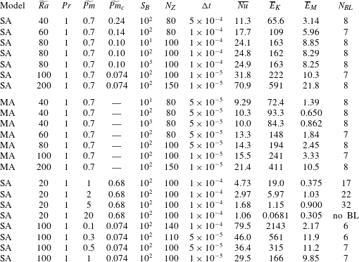
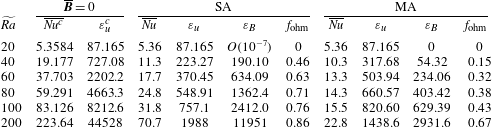
Details for the simulations presented.
 $N_{Z}$
is the number of Chebyshev points in the vertical direction and
 $N_{BL}$
is the approximate number of Chebyshev points within the time-averaged thermal
 $\unicode[STIX]{x1D6E9}$
boundary layer, denoted BL. The time discretization for the mean magnetic field is given by
 $\unicode[STIX]{x0394}\unicode[STIX]{x1D70F}=S_{B}\unicode[STIX]{x0394}t$
. The time steps result in converged solutions, although they are not optimized during the runs, meaning larger time steps are likely possible. The critical magnetic Prandtl number
 $\widetilde{Pm}_{c}$
indicates the
 $\widetilde{Pm}$
above which a kinematic dynamo can exist (calculated for the SA kinematic model in Calkins et al.
Reference Calkins, Julien, Tobias, Aurnou and Marti2016a
). Additional runs with varying
 $\widetilde{Pm}$
were calculated, but the energetics are unchanged from those reported in the paper.

2.4 Time stepping considerations
Time stepping the mean temperature equation introduces an issue with the length of simulations. For instance, the time required for the mean temperature to have diffused through the vertical layer is
 $O(E^{-2/3}t)$
. The simulation length therefore becomes computationally prohibitive as
 $E$
is lowered even for this simplified one-dimensional problem; for the Earth’s outer core, where
 $E=O(10^{-15})$
, this requires a simulation to be carried out to a fast convective time
 $t=O(10^{10})$
for one large-scale magnetic diffusion time. However, in the purely hydrodynamic regime the mean temperature in the single mode system achieves a steady state where
 $\unicode[STIX]{x2202}_{T}\overline{\overline{\unicode[STIX]{x1D703}}}^{\unicode[STIX]{x1D70F}}=0$
(Julien & Knobloch Reference Julien and Knobloch1998). Adopting this as an a priori constraint resolves the issue associated with the simulation length by significantly reducing the time required to reach the steady state.
In the present work, the existence of magnetic fields and the associated mean magnetic evolution time scale
 $\unicode[STIX]{x1D70F}=\unicode[STIX]{x1D716}^{3/2}t$
represent an added complexity in pursuing the aforementioned a priori constraint. However, this constraint may be achieved as follows (see appendix A for further details). The composite mean temperature equation from which the multiscale decomposition (2.7) and (2.8) are deduced is given by the
 $O(\unicode[STIX]{x1D716}^{2})$
ordered term
 $$\begin{eqnarray}\unicode[STIX]{x2202}_{T}\overline{\overline{\unicode[STIX]{x1D703}}}^{\unicode[STIX]{x1D70F}}+\unicode[STIX]{x2202}_{\unicode[STIX]{x1D70F}}\overline{\unicode[STIX]{x1D703}}+\unicode[STIX]{x2202}_{Z}(\overline{w\unicode[STIX]{x1D703}^{\prime }})=\frac{1}{Pr}\unicode[STIX]{x2202}_{ZZ}\overline{\overline{\unicode[STIX]{x1D703}}}^{\unicode[STIX]{x1D70F}}.\end{eqnarray}$$
On defining the composite temperature
 $\overline{\unicode[STIX]{x1D703}}(Z,\unicode[STIX]{x1D70F},T)=\overline{\overline{\unicode[STIX]{x1D703}}}^{\unicode[STIX]{x1D70F}}(Z,T)+\unicode[STIX]{x1D716}^{1/2}\overline{\unicode[STIX]{x1D717}}(Z,\unicode[STIX]{x1D70F},T)$
, we obtain
 $$\begin{eqnarray}\unicode[STIX]{x2202}_{T}\overline{\unicode[STIX]{x1D703}}+\unicode[STIX]{x2202}_{Z}(\overline{w\unicode[STIX]{x1D703}^{\prime }})=\frac{1}{Pr}\unicode[STIX]{x2202}_{ZZ}\overline{\unicode[STIX]{x1D703}}+O(\unicode[STIX]{x1D700}^{1/2}).\end{eqnarray}$$
An instantaneous evolution equation for the mean temperature may be obtained by commuting the differential operators of (2.65) into the kernel of the averaging operator (2.3). The instantaneous temperature equation is obtained by constraining the kernel to be zero (details of this can be found in appendix A), leaving
 $$\begin{eqnarray}\unicode[STIX]{x1D716}^{-2}\unicode[STIX]{x2202}_{t}\overline{\unicode[STIX]{x1D703}}^{{\mathcal{V}}}+\unicode[STIX]{x2202}_{Z}(\overline{w\unicode[STIX]{x1D703}^{\prime }}^{{\mathcal{V}}})=\frac{1}{Pr}\unicode[STIX]{x2202}_{ZZ}\overline{\unicode[STIX]{x1D703}}^{{\mathcal{V}}},\end{eqnarray}$$
where
 $\overline{f}^{{\mathcal{V}}}$
denotes averaging over small spatial scales. The single mode mean temperature equations (2.29) in the SA model and (2.45) in the MA model are deduced from this equation. Invoking the steady state approximation
 $\unicode[STIX]{x1D716}^{-2}\unicode[STIX]{x2202}_{t}\overline{\unicode[STIX]{x1D703}}^{{\mathcal{V}}}=0$
implies
 $$\begin{eqnarray}\unicode[STIX]{x2202}_{Z}(\overline{w\unicode[STIX]{x1D703}^{\prime }}^{{\mathcal{V}}})=\frac{1}{Pr}\unicode[STIX]{x2202}_{ZZ}\overline{\unicode[STIX]{x1D703}}^{{\mathcal{V}}}\quad \text{and}\quad Nu(t,\unicode[STIX]{x1D70F},T)=Pr(\overline{w\unicode[STIX]{x1D703}^{\prime }}^{{\mathcal{V}}})-\unicode[STIX]{x2202}_{Z}\overline{\unicode[STIX]{x1D703}}^{{\mathcal{V}}}.\end{eqnarray}$$
Time averaging these instantaneous relations gives the relations for intermediate and slow time scale variations over
 $t,\unicode[STIX]{x1D70F}$
 $$\begin{eqnarray}\unicode[STIX]{x2202}_{Z}(\overline{w\unicode[STIX]{x1D703}^{\prime }})=\frac{1}{Pr}\unicode[STIX]{x2202}_{ZZ}\overline{\unicode[STIX]{x1D703}}\quad \text{and}\quad Nu(\unicode[STIX]{x1D70F},T)=Pr(\overline{w\unicode[STIX]{x1D703}^{\prime }})-\unicode[STIX]{x2202}_{Z}\overline{\unicode[STIX]{x1D703}},\end{eqnarray}$$
 $$\begin{eqnarray}\unicode[STIX]{x2202}_{Z}(\overline{\overline{w\unicode[STIX]{x1D703}^{\prime }}}^{\unicode[STIX]{x1D70F}})=\frac{1}{Pr}\unicode[STIX]{x2202}_{ZZ}\overline{\overline{\unicode[STIX]{x1D703}}}^{\unicode[STIX]{x1D70F}}\quad \text{and}\quad Nu(T)=Pr(\overline{\overline{w\unicode[STIX]{x1D703}^{\prime }}}^{\unicode[STIX]{x1D70F}})-\unicode[STIX]{x2202}_{Z}\overline{\overline{\unicode[STIX]{x1D703}}}^{\unicode[STIX]{x1D70F}}.\end{eqnarray}$$
The a priori assumption
 $\unicode[STIX]{x2202}_{T}\overline{\overline{\unicode[STIX]{x1D703}}}_{0}^{\unicode[STIX]{x1D70F}}=0$
is compatible with (2.69) and indicates that
 $Nu(T)=Nu$
is a stationary value. Moreover, the above results also indicate that the variation of the heat transport about the stationary value is given by
 $$\begin{eqnarray}Nu(\unicode[STIX]{x1D70F},T)-Nu=Pr(\overline{w\unicode[STIX]{x1D703}^{\prime }}-\overline{\overline{w\unicode[STIX]{x1D703}^{\prime }}}^{\unicode[STIX]{x1D70F}})+O(\unicode[STIX]{x1D700}^{1/2}).\end{eqnarray}$$
This variation in the convective heat flux can admit oscillations with a frequency on the mean inductive time scale. Thus, as
 $E$
is lowered, oscillations that occur should show longer periods. Notably, (2.70) implies no a priori bounds for the amplitude of the variation.
Similar to the analysis and discussion of the mean temperature time scale, a large number of fast convective time steps are required to reach a mean magnetic diffusion time
 $\unicode[STIX]{x1D70F}=E^{1/2}t$
because of the scale separation between the fast convective time and the mean magnetic evolution time. For an Ekman number of
 $E=10^{-6}$
, a fast convective time of
 $t=O(10^{3})$
is required to reach
 $\unicode[STIX]{x1D70F}=O(1)$
. With a time step size of
 $\unicode[STIX]{x0394}t=10^{-5}$
, which is characteristic of many of our cases detailed in table 1, this yields a total of
 $10^{8}$
time steps. However, to reduce computation time, the simulations are considered converged if statistically stationary results are obtained for the Nusselt number and magnetic energy upon time averaging.
2.5 Multiscale time stepping strategies
Obtaining numerical solutions to the QGDM requires specialized numerical techniques given the presence of multiple time scales in the governing equations. In particular, temporal discretization of the QGDM implies that averaging must also be performed in a discretized fashion, and the primary issue then becomes determining the appropriate averaging time scale, or window. Several methods are in current use for obtaining numerical solutions to temporally multiscale equations, though the choice of the method employed depends strongly on the detailed form of the equations and significant testing is required to determine which method best suits the particular problem (e.g. E et al. Reference E, Engquist, Li, Ren and Vanden-Eijnden2007; Haut & Wingate Reference Haut and Wingate2014). Below we discuss the two different techniques that are used in the present work.
2.5.1 The stiff method
One method for treating the different time scales numerically is to directly simulate the time derivatives in (2.4)–(2.11) with their form written in terms of
 $\unicode[STIX]{x1D716}$
and the convective time derivative. This requires commuting time averaging with differential operators as outlined in appendix A. The single mode approximation then results in the SA and MA models given in §§ 2.1.1 and 2.1.2. Recall that we apply a steady state approximation for the mean heat equation so no time derivative remains in the mean temperature equation. Since the derivation of the QGDM requires
 $\unicode[STIX]{x1D716}\ll 1$
, the small
 $\unicode[STIX]{x1D716}$
parameter in the governing equations leads to a numerically stiff problem and we refer to the use of this common-in-time technique simply as the stiff method.
2.5.2 The heterogeneous multiscale method
A common method for the numerical treatment of multiscale equations is the so-called heterogeneous multiscale method (HMM) (E et al.
Reference E, Engquist, Li, Ren and Vanden-Eijnden2007). This method, which incorporates time scale separation, has previously been applied to asymptotic equations for wind-driven oceanic flows (e.g. Malecha, Chini & Julien Reference Malecha, Chini and Julien2014). In the present context, the HMM consists of time stepping the mean equations on specified large intervals of the fast time scale. We refer to this as the multiscale method. Specifically, the mean magnetic field is updated every
 $S_{B}$
convective time steps. Thus, the time discretization for the mean magnetic field is given by
 $\unicode[STIX]{x0394}\unicode[STIX]{x1D70F}=S_{B}\unicode[STIX]{x0394}t$
. The nonlinear terms in the mean magnetic field equations are averaged over all the fast convective time steps in each
 $\unicode[STIX]{x0394}\unicode[STIX]{x1D70F}$
time interval. Appropriate values for
 $S_{B}$
can be related back to the Ekman number,
 $E=\unicode[STIX]{x1D716}^{3}$
, by recalling the relation between the slow and fast time scales such that
 $$\begin{eqnarray}S_{B}=O(\unicode[STIX]{x1D716}^{-3/2})=O(E^{-1/2}).\end{eqnarray}$$
2.6 Stiff versus multiscale
We find that the stiff and multiscale methods lead to identical results when relation (2.71) is satisfied, though minor differences can appear when converting
 $S_{B}$
to an integer value. That both methods yield the same solutions is encouraging and allows for either method to be used, yet there are a few important points to note. The multiscale method requires fewer linear solves than the stiff method, since the mean magnetic field equations are only solved after a specified number of fast time steps. In general, however, we find that the multiscale method requires (for numerical stability) slightly smaller convective time step sizes than the stiff method. For instance, the SA model with
 $\widetilde{Ra}=40$
,
 $Pr=1$
and
 $S_{B}=10$
requires
 $\unicode[STIX]{x0394}t\leqslant 8\times 10^{-3}$
for the multiscale method, whereas the stiff method is numerically stable for
 $\unicode[STIX]{x0394}t\leqslant 1\times 10^{-2}$
. At the slightly larger Rayleigh number with
 $\widetilde{Ra}=60$
, the multiscale method requires
 $\unicode[STIX]{x0394}t\leqslant 3.5\times 10^{-3}$
for numerical stability while the stiff method can use
 $\unicode[STIX]{x0394}t\leqslant 6\times 10^{-3}$
. Given that the stiff method requires 2 extra matrix solves roughly every step (for
 $S_{B}$
large), the resulting computational cost is comparable but slightly favours the stiff method for the
 $\widetilde{Ra}=60$
case.
The difference in permissible time step sizes for the two methods indicates that the stiff method becomes more efficient for use at higher
 $\widetilde{Ra}$
. This benefit could be related to the averages used for the nonlinear terms in the mean magnetic equations in the multiscale method, whereas in the stiff technique the nonlinear terms are updated at each time step. We note that there are a multitude of different HMM techniques, including some that decouple
 $\unicode[STIX]{x0394}t$
and
 $\unicode[STIX]{x0394}\unicode[STIX]{x1D70F}$
and focus solely on the slow dynamics. In such cases, the fast dynamics is run until a stationary state producing stable averages is achieved (see Malecha et al.
Reference Malecha, Chini and Julien2014). This approach enables larger numerical time steps for the slow dynamics, such that the multiscale method becomes more efficient. Since we are interested in both continuous fast and slow dynamics and want to understand how they are coupled, we choose to keep our time stepping linked through these parameters (
 $E$
or
 $S_{B}$
), rather than a condition based on a minimal time to acquire a stationary state. In the remainder of this work, we report results from the multiscale method only, since both methods yield the same results.
3 Results
We have carried out a broad suite of simulations (runs) of the SA model, the MA model and the single amplitude, non-magnetic, hydrodynamic model (setting
 $\overline{\boldsymbol{B}}=0$
in the SA model). Various details of the simulations are provided in table 1. For all cases presented we fix the wavenumber
 $k$
to be that corresponding to the critical wavenumber
 $k_{c}$
for the onset of convection. In the present work we restrict the simulations to
 $Pr=1$
and therefore use the wavenumber
 $k=k_{c}=1.3048$
associated with steady convection (Chandrasekhar Reference Chandrasekhar1961). For
 $Pr\lesssim 0.68$
the onset of convection is oscillatory. In preliminary simulations with
 $Pr=0.1$
we found that the time stepping and averaging methods employed in the present work were unsatisfactory in the sense that no convergence of statistics was observed as the time-averaging window of the mean magnetic field (
 $S_{B}$
) was varied. We attribute this behaviour to the periodic dynamics that occurs for low Prandtl number fluids; capturing accurate statistics requires a more sophisticated averaging procedure since the position (in time) of the averaging window has a significant influence on the resulting average. In particular, significant errors in averaged quantities of periodic signals are introduced when averaging over non-integer multiples of the fundamental period of oscillation. Identifying the period of oscillation a priori is not possible for nonlinear dynamo solutions. For these reasons we leave the analysis of low Prandtl number dynamos for future work. Simulations with higher
 $Pr=10$
displayed qualitatively similar results to the
 $Pr=1$
case, albeit with higher
 $\widetilde{Ra}$
transitions to unsteady dynamics due to the increased importance of viscosity for higher
 $Pr$
. Additional
 $Pr=1$
runs with fixed
 $\widetilde{Ra}=20,100$
and varied
 $\widetilde{Pm}$
show similar energetics.
3.1 Determination of the emf-averaging window,
 $S_{B}$

We find a posteriori that the influence of changing the averaging window
 $S_{B}\unicode[STIX]{x0394}t$
in the mean induction equation on the resulting dynamo solutions depends on several factors: the model used (SA or MA); the type of convection (steady or oscillatory); and the value of
 $\widetilde{Ra}$
(indicating flow supercriticality). To simplify the presentation, only the fast convective time
 $t$
is used in plots presenting time-dependent data.
The simplest solutions that we find are those that correspond to steady convection. Steady convection is found at sufficiently low combinations of
 $\widetilde{Ra}$
and
 $\widetilde{Pm}$
values and yields steady values of the magnetic energy
 $E_{M}$
for all interval lengths
 $S_{B}$
. In general, the values of (
 $\widetilde{Ra},\widetilde{Pm}$
) for which these steady solutions are achieved varies. For example,
 $\widetilde{Ra}=20$
produces steady solutions for all
 $\widetilde{Pm}\leqslant 20$
, whereas
 $\widetilde{Ra}=100$
is only steady for runs with
 $\widetilde{Pm}\leqslant 0.4$
. Although
 $E_{M}$
is constant for steady convection solutions, changing
 $S_{B}$
affects the periodicity of the individual components
 $\langle \overline{B}_{x}^{2}(t)\rangle ^{1/2}$
,
 $\langle \overline{B}_{y}^{2}(t)\rangle ^{1/2}$
. While we label these as steady results due to the fact that
 $\overline{B}_{x}^{2}+\overline{B}_{y}^{2}$
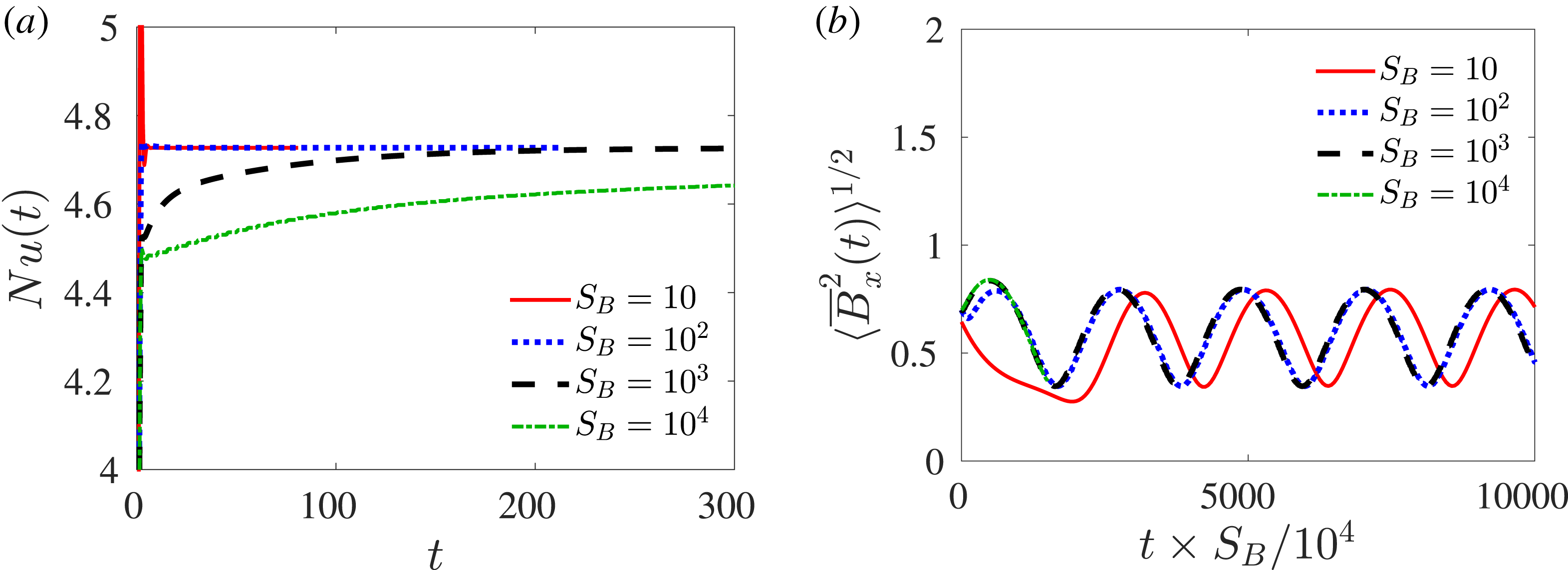
reaches a constant value, the dynamos are oscillatory for all cases. An example of these steady solutions is illustrated in figure 1, where the Nusselt number
 $Nu$
settles to a constant value for all
 $S_{B}$
. However, as
 $E$
is decreased (and
 $S_{B}$
is increased), the result requires a longer simulation time to reach equilibrium. The runs presented in figure 1(b) have been rescaled to demonstrate self-similarity of the solutions. Each run at a given
 $S_{B}$
has been multiplied by the factor needed to match the time scale of the
 $S_{B}=10^{4}$
run; for example, the
 $S_{B}=10^{2}$
run has been scaled by
 $10^{2}$
. For these steady cases, the choice of
 $S_{B}$
is irrelevant since time-averaged quantities such as the emf and Nusselt number do not change with time.
Plots illustrating the influence of the mean magnetic field averaging length
 $S_{B}$
on both (a) the Nusselt number
 $Nu$
and (b)
 $\langle \overline{B}_{x}^{2}(t)\rangle ^{1/2}$
. The interval length
 $S_{B}$
denotes the number of fast convective time steps over which the mean magnetic field equations are held constant and the nonlinear terms in the mean induction equations are averaged. All results were obtained with
 $\widetilde{Ra}=20$
,
 $Pr=1$
and
 $\widetilde{Pm}=1$
. The time in (b) has been scaled by
 $S_{B}/10^{4}$
to highlight the temporal self-similarity of all the runs.

The results show more complex dependence on
 $S_{B}$
when the underlying convection is unsteady. We find that the value of
 $S_{B}$
becomes critical to capturing self-similar behaviour, which we consider to be indicative of capturing physically correct behaviour. Therefore, the results are deemed ‘converged’ if self-similar behaviour is identified, where self-similar behaviour implies reaching the same statistically steady results for
 $\overline{Nu}$
and
 $\overline{E}_{M}$
. Unsteady convective dynamics appears as
 $\widetilde{Ra}$
is increased, where the precise value of
 $\widetilde{Ra}$
at which unsteady motions occur depends on both
 $Pr$
and
 $\widetilde{Pm}$
. Above the transition to unsteady motions, the hydrodynamic component of these flows becomes oscillatory with a single frequency for sufficiently small
 $\widetilde{Ra}$
. Additional frequencies in both the convection and mean magnetic field are then generated as
 $\widetilde{Ra}$
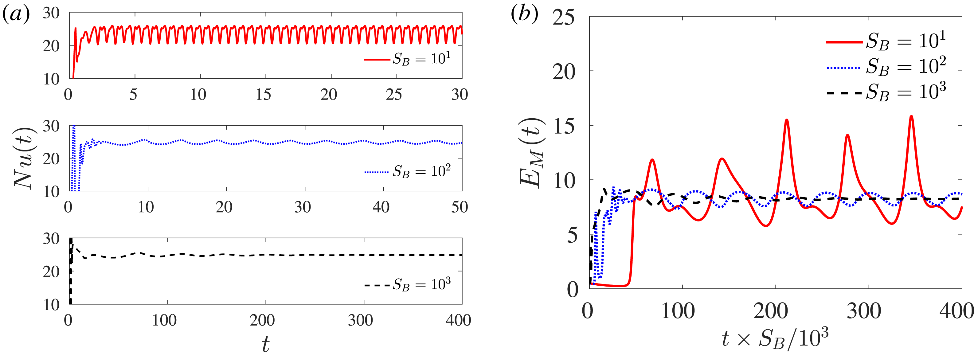
is increased further until chaotic convection is observed for sufficiently high reduced Rayleigh number. An example of a case with periodic oscillations is shown in figure 2 for several values of
 $S_{B}$
. We note that (2.70) implies variability in the heat transfer on the
 $\unicode[STIX]{x1D70F}$
time scale; as such an
 $\unicode[STIX]{x1D716}$
-dependent increase is observed in the period of oscillations in the Nusselt number on an
 $O(\unicode[STIX]{x1D716}^{-3/2})$
scale with a constant of proportionality
 ${\sim}1/20$
(for the
 $S_{B}=10^{3}$
run). Additionally, the magnetic energy shows self-similar behaviour in time for the longer
 $S_{B}=10^{2},10^{3}$
runs, with consistent averages despite the fact that the amplitudes of the oscillations in
 $E_{M}$
decrease with increasing
 $S_{B}$
, settling to a constant value for the
 $S_{B}=10^{3}$
run. For
 $Pr=10$
we observe the same behaviour in the dynamics on
 $S_{B}$
. The
 $Pr=10$
case also displays both the transition to unsteady convection for higher
 $\widetilde{Ra}$
, and the requirement of longer
 $S_{B}$
intervals for self-similar behaviour of the runs.
Comparison of (a) the Nusselt number
 $Nu(t)$
and (b) the magnetic energy
 $E_{M}(t)$
versus the fast convective time
 $t$
, for three different values of
 $S_{B}$
using the single amplitude (SA) model. The simulation parameters are
 $\widetilde{Ra}=80$
,
 $Pr=1$
and
 $\widetilde{Pm}=0.7$
. The oscillations that are observed in
 $Nu$
decrease in amplitude and increase in period as
 $S_{B}$
is increased.

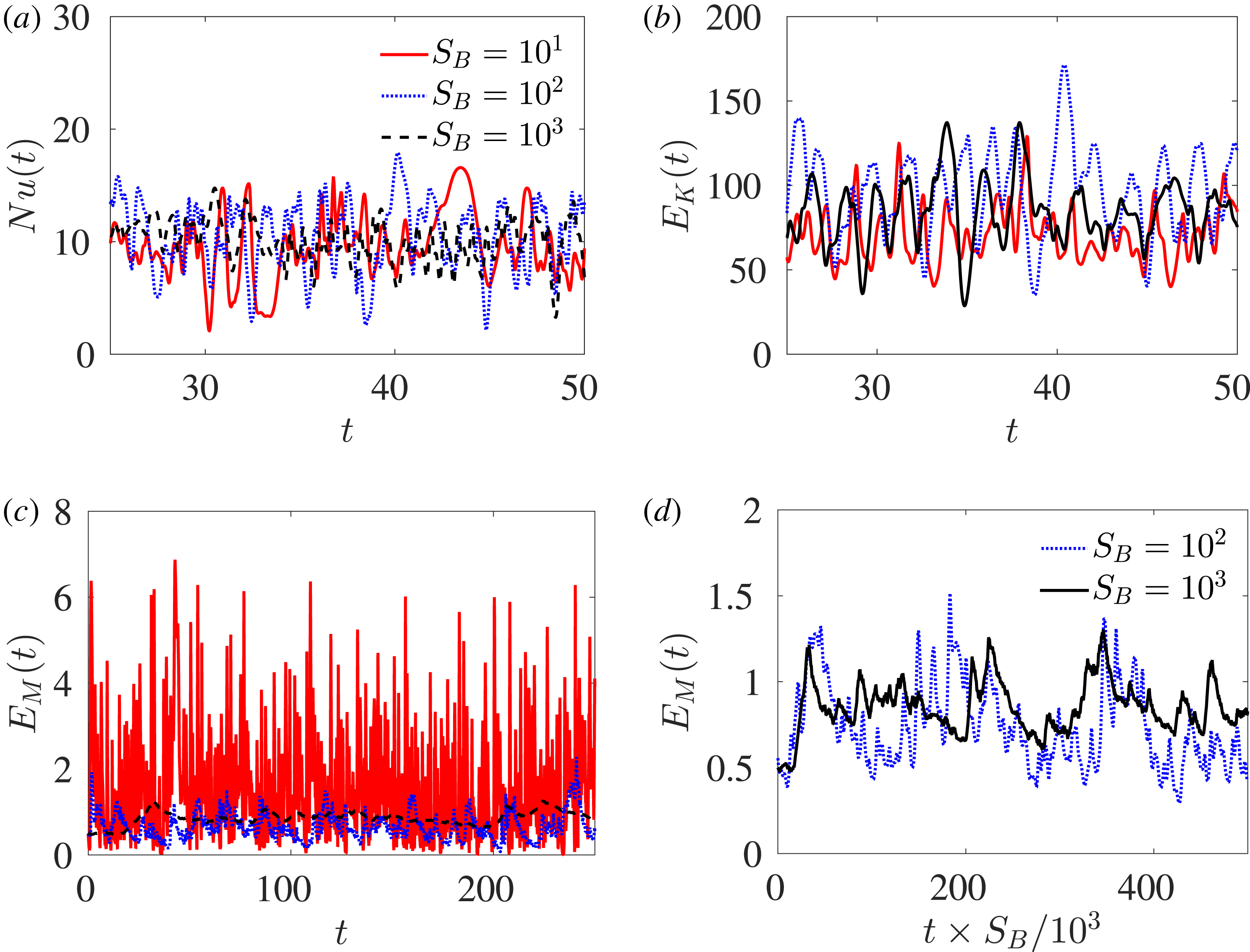
In comparison to the SA model, the results from the MA are more physically rich in both their time dependence and spatial (
 $Z$
) structure (figure 3). Whereas the
 $Nu(t)$
and
 $E_{K}(t)$
results shown in figures 3(a) and 3(b), respectively, exhibit similar behaviour for the three values of
 $S_{B}$
, figure 3(c) shows that significant differences in the magnetic energy
 $E_{M}$
appear for different values of
 $S_{B}$
. These results illustrate that it is insufficient to rely on the behaviour of a single quantity when determining if the results converge, or exhibit self-similar behaviour, with increasing
 $S_{B}$
. Figure 3(d) shows the magnetic energy for only the two largest values of
 $S_{B}$
over scaled time; here we observe similar temporal dependence and amplitudes of
 $E_{M}$
for the two cases, suggesting that
 $S_{B}=10^{2}$
is sufficient to capture the correct dynamics. We attribute these differences to a lack of sufficient temporal scale separation in the sense that the equivalent value of
 $E$
is too large, as was also observed in the
 $\widetilde{Ra}=80$
SA case shown in figure 2. The spatial structure of the solutions confirms this as the time-averaged vertical profiles of the two longer cases agree, while the
 $S_{B}=10$
result shows slight differences in the interior structure.
Results illustrating the influence of
 $S_{B}$
for the mixed amplitude (MA) model. The quantities shown are (a) Nusselt number
 $Nu(t)$
; (b) kinetic energy
 $E_{K}(t)$
; (c) magnetic energy
 $E_{M}(t)$
; and (d) magnetic energy
 $E_{M}(t)$
with rescaled time. The parameters are
 $\widetilde{Ra}=40$
,
 $Pr=1$
and
 $\widetilde{Pm}=0.7$
for
 $S_{B}=10^{1},10^{2}$
and
 $10^{3}$
. While all of the
 $Nu$
and
 $E_{K}$
results appear similar, there is a visible difference in the magnetic energy results between the
 $S_{B}=10^{1}$
results and the larger
 $S_{B}$
cases. Plot (d) highlights similarities in
 $E_{M}$
for the two largest values of
 $S_{B}$
, where the
 $S_{B}=10^{2}$
run time has been scaled by 10 and begins after the initial transient.

In all of the results that follow we set
 $S_{B}=10^{2}$
(see table 1). This value of
 $S_{B}$
was chosen because lower
 $S_{B}$
runs take less time to reach a statistically stationary state, and all of the tested cases show that the
 $S_{B}=10^{2}$
results are similar to the higher
 $S_{B}$
results as the time-averaged quantities agree with higher
 $S_{B}$
metrics.
3.2 Increasing the convective supercriticality
We examine the effect of increasing the convective supercriticality over the range of
 $20\leqslant \widetilde{Ra}\leqslant 200$
(see table 1) for a fixed value of
 $\widetilde{Pm}$
. The magnetic energy
 $E_{M}$
and kinetic energy
 $E_{K}$
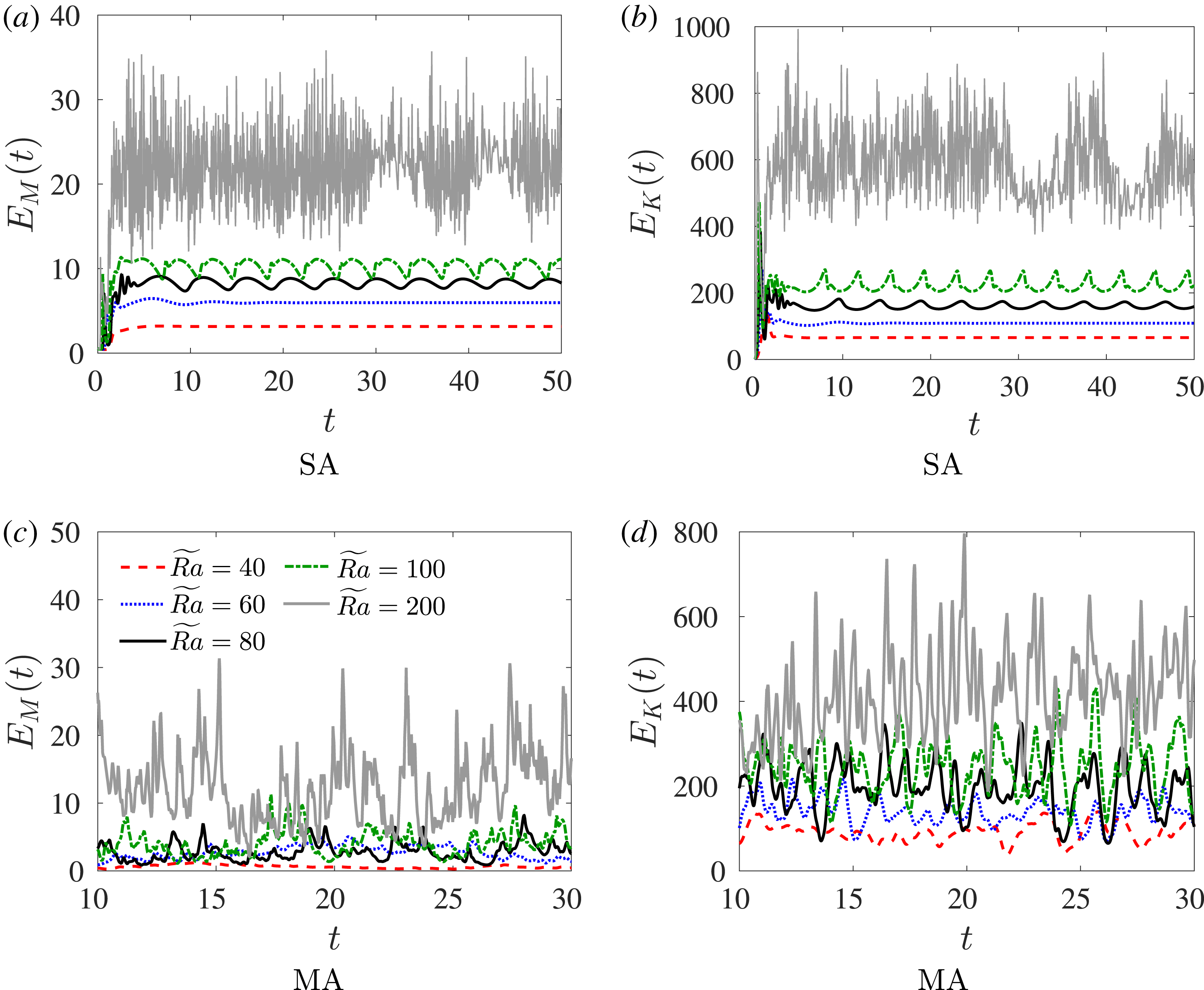
, shown in figure 4, illustrate the oscillations that are found in dynamo solutions as
 $\widetilde{Ra}$
is increased for the SA model (upper row) and the MA model (lower row). Given that
 $E_{M}$
and
 $Nu$
are tied through the
 $\overline{B}_{x}^{2}+\overline{B}_{y}^{2}$
term that contributes to the Lorentz force in the
 $\unicode[STIX]{x1D6F9}$
and
 $W$
equations, oscillations in the convective dynamics naturally lead to oscillations in the magnetic field. Evident from the
 $\widetilde{Ra}=80,100$
results in figure 4(a,b) is the inverse relationship between
 $E_{M}$
and
 $E_{K}$
.
The instantaneous magnetic energy
 $E_{M}(t)$
and kinetic energy
 $E_{K}(t)$
for the SA model (a,b) and MA model (c,d) for various values of
 $\widetilde{Ra}$
. Oscillations appear as
 $\widetilde{Ra}$
is increased in the SA model, losing periodicity for
 $\widetilde{Ra}=200$
, and all the MA model results show large fluctuations. The parameters are
 $Pr=1$
,
 $\widetilde{Pm}=0.7$
and
 $S_{B}=10^{2}$
. Different vertical and horizontal axes ranges are used to more clearly display the MA results.

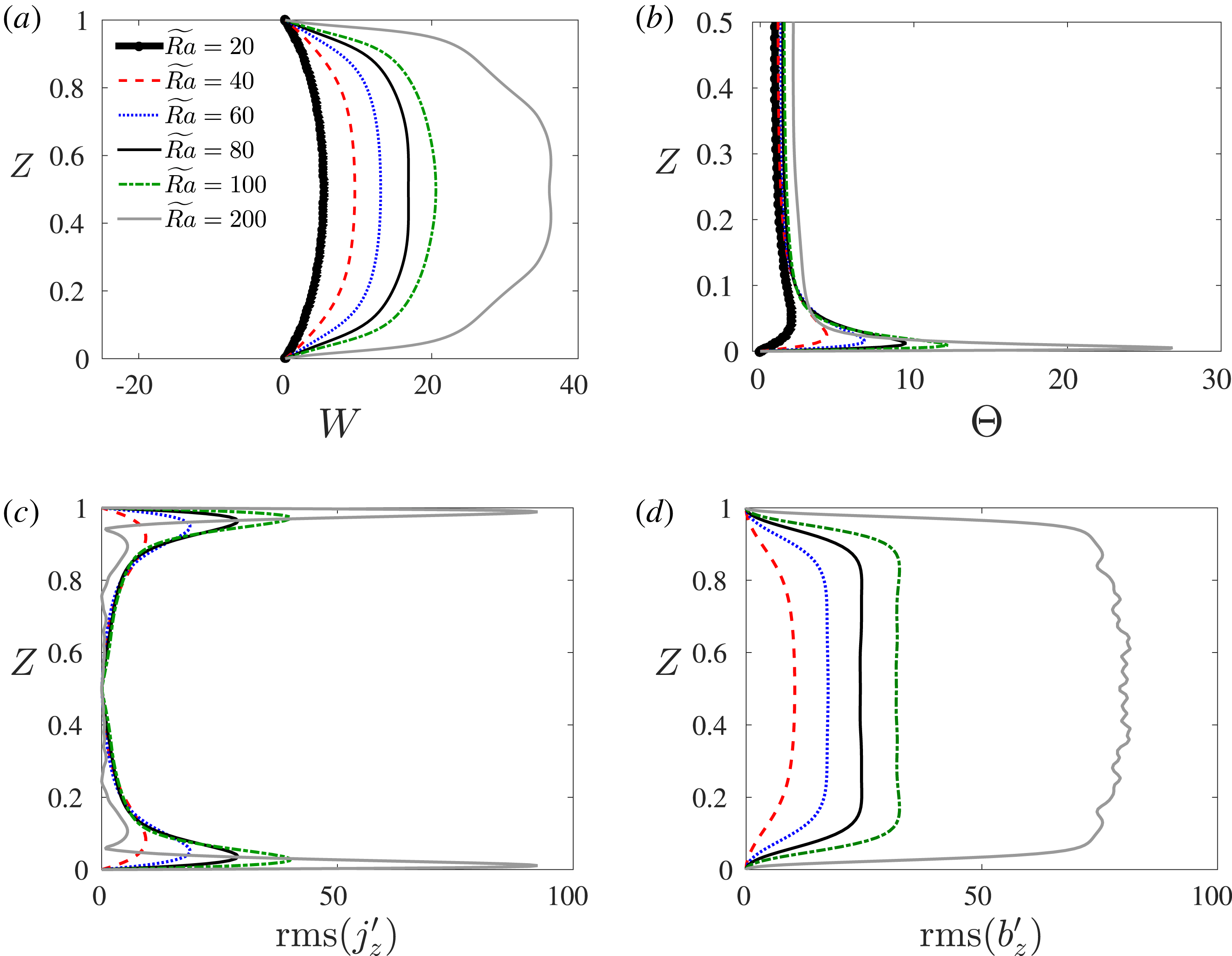
Profiles showing the vertical structure of the fluctuating quantities in the SA model are given in figure 5 for a range of Rayleigh numbers. As expected, both
 $W$
and
 $b_{z}^{\prime }$
show a growing amplitude with
 $\widetilde{Ra}$
, and the fields
 $\unicode[STIX]{x1D6E9}$
and
 $j_{z}^{\prime }$
show the development of boundary layers that decrease in width with increasing
 $\widetilde{Ra}$
. In comparison to non-magnetic convection, the magnitude of all hydrodynamic quantities (
 $W,\unicode[STIX]{x1D6F9},\unicode[STIX]{x1D6E9}$
) is diminished due to the conversion of kinetic energy into magnetic energy.
Vertical profiles for various r.m.s. quantities of the SA model with
 $\widetilde{Pm}=0.7$
,
 $Pr=1$
,
 $S_{B}=10^{2}$
and various
 $\widetilde{Ra}$
; (a) vertical velocity; (b) fluctuating temperature; (c) vertical fluctuating current density; and (d) vertical fluctuating magnetic field. To better display the thermal boundary layers only the lower half of the
 $\unicode[STIX]{x1D6E9}$
profile is shown in (b). Profiles in (c,d) are averaged in time for all
 $\widetilde{Ra}$
and the
 $W,\unicode[STIX]{x1D6E9}$
profiles for
 $\widetilde{Ra}=80,100,200$
are averaged in time.

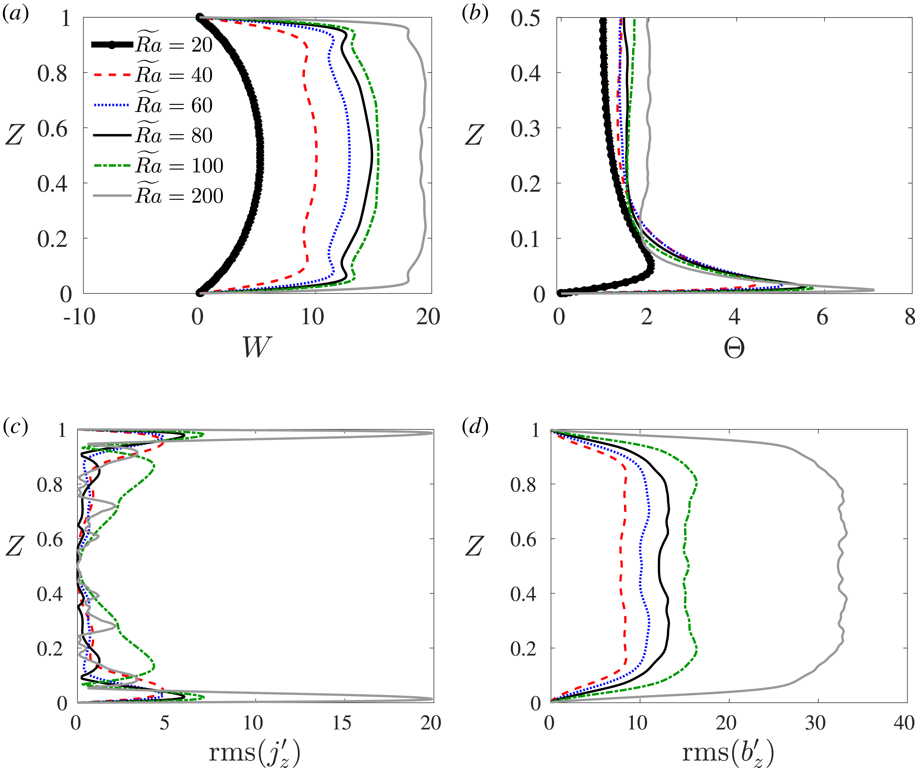
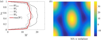
Typical profiles of MA dynamo solutions are shown in figure 6(a,b). The solutions do not settle to an equal amplitude, e.g.
 $W_{1}=W_{2}=W_{3}$
, even when using initial conditions with each component equal to the SA solution. Thus, we observe that the subspace associated with the SA model is unstable. However, due to rotational invariance in the horizontal plane, it is expected that statistically these amplitudes should agree when adequate averaging is performed such that
 $W_{1}\approx W_{2}\approx W_{3}$
. Figure 7(a) shows comparisons of the
 $W$
profiles for the SA and MA dynamo models, including the individual components and the r.m.s. profile. The horizontal structure is displayed for the midplane of
 $W_{1}(Z)h_{1}(x,y)+W_{2}(Z)h_{2}(x,y)+W_{3}(Z)h_{3}(x,y)$
in figure 7(b) where the hexagonal structure is evident, although deviating slightly from a perfect hexagonal pattern.
Vertical profiles for various r.m.s. quantities of the MA model with
 $\widetilde{Pm}=0.7$
,
 $Pr=1$
,
 $S_{B}=10^{2}$
and various
 $\widetilde{Ra}$
; (a) vertical velocity; (b) fluctuating temperature; (c) vertical fluctuating current density; and (d) vertical fluctuating magnetic field. To better display the thermal boundary layers only the lower half of the
 $\unicode[STIX]{x1D6E9}$
profile is shown in (b). All of the profiles have been time averaged.

Comparison of (a) the vertical velocity profile
 $W$
and (b) the horizontal structure of the full
 $w=W(Z)\,h(x,y)$
field for the MA model at the midplane. (a) Shows the vertical profiles for the two classes of dynamo solutions; the separate amplitudes (
 $W_{1,2,3}$
) of the MA model are shown in grey, and the symmetrized r.m.s. profiles for the MA model and the SA are shown by the solid red and solid black curves, respectively. The horizontal structure of
 $w$
is shown in (b), where the hexagonal structure shows slight variations in the shape arising from the different amplitudes in each direction. The parameters are
 $\widetilde{Ra}=100$
,
 $Pr=1$
,
 $\widetilde{Pm}=0.7$
and
 $S_{B}=10^{2}$
.

The time-averaged profiles of the
 $x$
-component of the mean magnetic field are shown in figure 8. The mean magnetic field also forms boundary layers that progressively thin with increasing
 $\widetilde{Ra}$
. The mean magnetic field oscillates in time for all of the cases investigated here; however, as
 $\widetilde{Ra}$
is increased, a broad range of frequencies become excited which gives way to a complex temporal dependence even for these relatively simple single mode convection solutions.
Profiles of the r.m.s.
 $x$
-component of the mean magnetic field vector for (a) the SA model and (b) the MA model. The parameters are
 $\widetilde{Pm}=0.7$
,
 $Pr=1$
and
 $S_{B}=10^{2}$
.

Figure 9 shows the influence of
 $\widetilde{Ra}$
on the helicity for both (a) non-magnetic convection solutions and (b,c) magnetic solutions. As the thermal forcing increases, the anti-symmetric profiles form boundary layers which move closer to the boundaries and become narrower than the non-magnetic counterparts. These results are a clear indication that the convection is significantly modified by the presence of the magnetic field.
Relative helicity
 $\overline{{\mathcal{H}}}_{R}$
profiles for (a) non-magnetic (
 $\overline{\boldsymbol{B}}=0$
) convection and (b,c) dynamo solutions. The parameters are
 $\widetilde{Pm}=0.7$
,
 $Pr=1$
,
 $S_{B}=10^{2}$
and various
 $\widetilde{Ra}$
. The line markings for each
 $\widetilde{Ra}$
as listed in (a) also apply for (b,c). All profiles are anti-symmetric with respect to
 $Z$
so that only the lower half of each profile is displayed.

3.3 Dissipation and heat transfer
Comparison of these runs with non-magnetic convection reveals lower Nusselt numbers and larger magnitude interior mean temperature gradients for a fixed value of
 $\widetilde{Ra}$
(see figure 10
a,b). The non-magnetic case approaches an isothermal interior according to the scaling law
 $|\unicode[STIX]{x2202}_{Z}\overline{\unicode[STIX]{x1D703}}|\sim \widetilde{Ra}^{-1}$
(Sprague et al.
Reference Sprague, Julien, Knobloch and Werne2006), while the SA dynamos show a diminished exponent and the MA dynamos saturate at large Rayleigh numbers. Similarly, the kinetic energy is diminished from non-magnetic rotating convection single mode solutions, as shown in figure 10(c). Given that these results can be tied to the equality of power integrals in (2.57), the exchange and balance of energy can be understood through a comparison of the three figures. Since
 $Nu=\unicode[STIX]{x1D700}_{\unicode[STIX]{x1D6E9}}$
and
 $2k^{2}E_{K}=\unicode[STIX]{x1D700}_{u}$
, a scaling relation of
 $\unicode[STIX]{x1D700}_{\unicode[STIX]{x1D6E9}}^{c}\widetilde{Ra}^{1}\sim \unicode[STIX]{x1D700}_{u}^{c}$
is expected for the non-magnetic case where
 $\unicode[STIX]{x1D700}_{B}=0$
. Scaling
 $2k^{2}E_{K}=\unicode[STIX]{x1D700}_{u}\sim \widetilde{Ra}_{E_{K}}^{\unicode[STIX]{x1D6FC}}$
and
 $Nu=\unicode[STIX]{x1D700}_{\unicode[STIX]{x1D6E9}}\sim \widetilde{Ra}_{Nu}^{\unicode[STIX]{x1D6FD}}$
; figure 10(a,c) confirm the balance with
 $(\widetilde{Ra}_{Nu})^{1.5}\widetilde{Ra}^{1}=(\widetilde{Ra}_{E_{K}})^{2.5}$
. For the magnetic case, there must be a balance between the three terms in (2.57) since
 $\unicode[STIX]{x1D700}_{B}\neq 0$
. The SA model shows
 $\unicode[STIX]{x1D700}_{u}$
and
 $\unicode[STIX]{x1D700}_{\unicode[STIX]{x1D6E9}}$
are diminished from the non-magnetic case with scalings of
 $\widetilde{Ra}_{E_{K}}^{1.5}$
and
 $\widetilde{Ra}_{Nu}^{1.2}$
so that the non-magnetic balance is violated. This implies from (2.57) that
 $\unicode[STIX]{x1D700}_{B}$
must scale around
 $\widetilde{Ra}_{B}^{2.2}$
. The calculated scaling of the ohmic dissipation (not shown) is approximately
 $\unicode[STIX]{x1D700}_{B}\sim \widetilde{Ra}_{B}^{2.5}$
, indicating that ohmic dissipation is dominant over viscous dissipation in the fluid layer for high
 $\widetilde{Ra}$
. Figure 10(d) shows the fraction of ohmic dissipation, where it is observed that
 $\unicode[STIX]{x1D700}_{B}$
dominates over
 $\unicode[STIX]{x1D700}_{u}$
at large
 $\widetilde{Ra}$
for both the SA and MA models.
Heat transfer quantities and volume-integrated energies for the two classes of dynamo solutions and non-magnetic (
 $\overline{\boldsymbol{B}}=0$
) SA results: (a) Nusselt number
 $Nu$
; (b) mean temperature gradient at the vertical midplane
 $\unicode[STIX]{x2202}_{Z}\overline{\unicode[STIX]{x1D703}}(Z=0.5)$
; (c) kinetic energy
 $E_{K}$
; and (d) fraction of ohmic dissipation
 $f_{\text{ohm}}=\unicode[STIX]{x1D700}_{B}/(\unicode[STIX]{x1D700}_{B}+\unicode[STIX]{x1D700}_{u})$
. Results for the SA model are shown by circles, the MA model results are shown by triangles and non-magnetic convection results are denoted with a square. Here
 $Pr=1$
,
 $\widetilde{Pm}=0.7$
and
 $S_{B}=10^{2}$
. The
 $\widetilde{Ra}=20$
results closely align with the non-magnetic result, as it is barely above the critical threshold for dynamo action and the magnetic energy remains small. All other
 $\widetilde{Ra}$
results included are well above the threshold for dynamo action, with critical
 $\widetilde{Pm}_{c}$
values reported in column 5 of table 1.

The mean temperature profiles for a range of
 $\widetilde{Ra}$
are shown in figure 11 for the magnetic SA case (a) and the magnetic MA case (b). The SA cases resemble that of non-magnetic convection in which the mean temperature profiles become increasingly isothermal in the fluid interior and show the development of thin thermal boundary layers as the Rayleigh number is increased. In contrast, the MA cases show a more complicated dependence on
 $\widetilde{Ra}$
, where the interior mean temperature gradient saturates at large
 $\widetilde{Ra}$
, though the thermal boundary layers continue to thin with increasing
 $\widetilde{Ra}$
. Both dynamo solutions highlight the decreased efficiency of thermal mixing in the interior relative to the non-magnetic case. While it is known that the mean temperature gradient for non-magnetic single mode solutions does not saturate with increasing
 $\widetilde{Ra}$
, multimode simulations have demonstrated saturation for
 $Pr\leqslant 1$
(Julien et al.
Reference Julien, Knobloch, Rubio and Vasil2012a
).
Mean temperature profiles
 $\overline{\unicode[STIX]{x1D703}}$
for the (a) SA and (b) MA dynamo solutions and a range of
 $\widetilde{Ra}$
.

The dissipation relations for non-magnetic convection and the dynamo can be compared by setting
 $\widetilde{Ra}/Pr^{2}$
fixed and equal in both expressions (2.54) and (2.55). These expressions can then be rearranged and equated to indicate that
 $$\begin{eqnarray}\frac{\unicode[STIX]{x1D700}_{u}}{Nu-1}+\frac{\unicode[STIX]{x1D700}_{B}}{Nu-1}=\frac{\unicode[STIX]{x1D700}_{u}^{c}}{Nu^{c}-1}.\end{eqnarray}$$
Given that
 $\unicode[STIX]{x1D700}_{B}\geqslant 0$
, this can be written as an inequality
 $$\begin{eqnarray}\frac{\unicode[STIX]{x1D700}_{u}}{Nu-1}\leqslant \frac{\unicode[STIX]{x1D700}_{u}^{c}}{Nu^{c}-1}.\end{eqnarray}$$
To achieve this balance, there are three possibilities: (i)
 $\unicode[STIX]{x1D700}_{u}\leqslant \unicode[STIX]{x1D700}_{u}^{c}$
and
 $Nu\geqslant Nu^{c}$
, (ii)
 $\unicode[STIX]{x1D700}_{u}\boldsymbol{<}\unicode[STIX]{x1D700}_{u}^{c}$
and
 $Nu<Nu^{c}$
or (iii)
 $\unicode[STIX]{x1D700}_{u}>\unicode[STIX]{x1D700}_{u}^{c}$
and
 $Nu\boldsymbol{>}Nu^{c}$
. Here we use the bold
 $\boldsymbol{<}$
symbols to denote that the quantity must increase or decrease an amount large enough to compensate for an opposing increase or decrease; for instance, in the third case the relative increase in
 $\unicode[STIX]{x1D700}_{u}$
(which increases the fraction) must be compensated by the relative increase in
 $Nu$
to make the inequality in (3.2) hold.
In table 2, the decrease in both
 $\unicode[STIX]{x1D700}_{u}$
and
 $Nu$
, relative to the non-magnetic case, can be seen over the entire range of
 $\widetilde{Ra}$
, indicating that these runs are in case (ii). Upon substituting these values in to (3.2), we find the relationship is satisfied. Equality in (3.2) is only achieved when
 $\unicode[STIX]{x1D700}_{B}\approx 0$
as for the
 $\widetilde{Ra}=20$
,
 $\widetilde{Pm}=0.7$
case. These results indicate that in these single mode models dynamo action acts to throttle the heat flux through the layer.
Various quantities from the power integral relations given in (2.54) and (2.57) for a range of
 $\widetilde{Ra}$
with
 $\widetilde{Pm}=0.7$
,
 $Pr=1$
,
 $k=1.3048$
and
 $S_{B}=10^{2}$
. Here
 $\unicode[STIX]{x1D700}_{u}^{c}$
is the total viscous dissipation for non-magnetic convection, and
 $\unicode[STIX]{x1D700}_{u}$
and
 $\unicode[STIX]{x1D700}_{B}$
are the total viscous and ohmic dissipations for dynamo solutions. The fraction of ohmic dissipation is defined by
 $f_{\text{ohm}}=\unicode[STIX]{x1D700}_{B}/(\unicode[STIX]{x1D700}_{B}+\unicode[STIX]{x1D700}_{u})$
. Note that for
 $\widetilde{Ra}=20$
, the critical magnetic Prandtl number is
 $\widetilde{Pm}_{c}\approx 0.65$
.

Experimental studies of non-rotating convection in the presence of an imposed vertical magnetic field report a decrease in the heat transfer from the non-magnetic case (Cioni, Chaumat & Sommeria Reference Cioni, Chaumat and Sommeria2000; Aurnou & Olson Reference Aurnou and Olson2001). However, DNS results from self-consistent rotating dynamos have found that the heat transfer increases in the presence of magnetic forces relative to non-magnetic simulations (Stellmach & Hansen Reference Stellmach and Hansen2004; Christensen & Aubert Reference Christensen and Aubert2006). One possible explanation for the discrepancy between the change in
 $Nu$
of the present asymptotic model and the DNS dynamo results is that the fixed horizontal structure considered here eliminates this phenomenon. Our results indicate that the restructuring of the convective planform in the presence of a magnetic field is crucial for enhancing the heat transfer (Chandrasekhar Reference Chandrasekhar1961; Fearn Reference Fearn1979).
3.4 Intermittency
The Nusselt number (a) and magnetic energy (b) results for an MA run with
 $\widetilde{Ra}=40$
,
 $Pr=1$
,
 $\widetilde{Pm}=0.7$
and
 $S_{B}=10^{3}$
showing the time variability and intermittent bursts of increased
 $E_{M}$
in the runs. For this run, the mean magnetic diffusion time is
 $t=O(10^{3})$
.

Figure 12 shows the heat transfer and magnetic energy results from a MA model run with
 $\widetilde{Ra}=40$
,
 $Pr=1$
,
 $\widetilde{Pm}=0.7$
and
 $S_{B}=10^{3}$
that displays intermittent changes with time. While the results show large variations for the majority of the time, intermittent bursts of nearly periodic patterns appear at some intervals. Whereas the Nusselt number shown in figure 12(a) is characterized by smaller fluctuations during these periods, we observe large variations (bursts) in the magnetic energy (figure 12
b). This behaviour is generally consistent with our findings that the heat transfer is reduced in the presence of strong magnetic field for these single mode solutions. The bursts in activity appear over roughly
 $1/5S_{B}=1/5E^{-1/2}$
diffusion times. Throughout these bursts, the averaged Nusselt number and kinetic energy values decrease and the averaged magnetic energy increases in comparison to averages outside of these intermittent periods. The vertical structure functions show more variation between them during these bursts as well. Similar intermittent behaviour was observed in a recent DNS investigation (Bushby et al.
Reference Bushby, Käpylä, Masada, Brandenburg, Favier, Guervilly and Käpylä2018), though the DNS results were found for parameter values disparate from those considered here.
4 Conclusion
This study investigates the dynamics of the QGDM, which is a fully nonlinear dynamo model that is valid in the limit of low Rossby and low magnetic Prandtl numbers. This regime is relevant to the dynamics of Earth’s liquid outer core and planetary interiors and cannot currently be accessed through direct numerical simulation or laboratory experiments. Using the single mode technique of assuming periodic horizontal planforms characterized by a single horizontal wavenumber
 $k$
, the problem is reduced from three spatial dimensions to a single dimension in the vertical. While single mode solutions are known to be unstable in multimode simulations, they provide a useful comparison for more realistic dynamics (Sprague et al.
Reference Sprague, Julien, Knobloch and Werne2006). The dimensional simplification allows for a detailed examination of time stepping methods to handle the three intrinsic time scales within the QGDM and permits an investigation of self-consistent dynamo action resulting from a specialized class of solutions.
The mean temperature equation is handled instantaneously on the fast convective time scale to avoid the computationally demanding length of the vertical diffusion times that would be needed. This is achieved by factoring the time averaging over
 $t$
from the mean temperature equation (see appendix A). The mean induction equation is then tested with two multiscale methods: the common-in-time stiff approach where the induction time scale is converted to the convective time scale, i.e.
 $\unicode[STIX]{x2202}_{\unicode[STIX]{x1D70F}}=\unicode[STIX]{x1D716}^{-3/2}\unicode[STIX]{x2202}_{t}$
; and the heterogeneous multiscale approach, where the mean induction equations are updated at intervals of fast convective time specified by
 $S_{B}\unicode[STIX]{x0394}t$
and use the fast time averaging of Reynolds, convective and magnetic stresses from that interval. We find that both of these methods provide consistent results. Moreover, varying the time interval
 $S_{B}$
over which the induction equation is averaged shows that self-similar behaviour is reached for longer averaging windows, indicating that sufficient scale separation of the equations is necessary for this model. The dynamics, especially for the MA model, shows strong time dependence and smooth results rely on extensive time averaging of the solutions, despite reaching statistically steady heat transfer and magnetic energy results.
Although the single mode solutions represent a highly simplified class of solutions, they nevertheless yield complex spatio-temporal dynamics. For sufficiently large Rayleigh numbers, both classes of solutions (SA and MA) yield chaotic dynamos with a broad range of time scales. Moreover, in contrast to previous kinematic investigations of the QGDM, the present work demonstrates that the dynamo-generated magnetic field has a strong influence on the structure and dynamics of the convection. The helicity of the flow is strongly modified and gives rise to magnetic fields that differ substantially in both spatial structure and temporal behaviour from the kinematic solutions.
All the dynamo solutions found in the present study show a decrease in the heat transfer relative to non-magnetic solutions at the same Rayleigh number. In contrast, DNS investigations (e.g. Stellmach & Hansen Reference Stellmach and Hansen2004; Christensen & Aubert Reference Christensen and Aubert2006) generally find the opposite effect whereby the heat transfer is increased in the presence of magnetic field. There is no formal proof that either case should be preferred. It is likely that our decreased heat transfer results are a consequence of the single mode, fixed horizontal planform solutions assumed in the present work. Our results therefore suggest that the restructuring of the convective planform (the single wavenumber, hexagonal horizontal structure assumed in the ansatz) plays a critical role in allowing enhanced heat transfer. This restructuring could occur either through the complete restructuring of the planform, modification of the dominant horizontal wavenumber, or a combination of these two effects.
A detailed investigation of the dissipation mechanisms in the single mode solutions shows that at sufficiently large Rayleigh numbers ohmic dissipation dominates over viscous dissipation. The solutions show a monotonic increase of the fraction of ohmic dissipation
 $f_{\text{ohm}}$
with increasing
 $\widetilde{Ra}$
. In general, both plane layer (Tilgner Reference Tilgner2014) and spherical (Christensen & Aubert Reference Christensen and Aubert2006) DNS studies find a non-monotonic dependence of
 $f_{\text{ohm}}$
on the thermal forcing. At present, it is unclear why such behaviour occurs, though we speculate that it may be related to the loss of rotational dominance in some cases due to the finite values of the Ekman numbers employed in DNS. Our results show that viscous dissipation plays a minor role in the heat transfer for increased forcing. Thus, the model is not categorically viscously dominated, despite the presence of a single, viscously selected horizontal scale that induces the dynamo.
By construction, the QGDM is designed to operate in the regime of low
 $Ro$
and low
 $Pm$
, a regime currently challenging for DNS and laboratory experiments to probe. Accordingly, this model provides results that cannot truly be compared with current direct numerical simulations, which remain limited to higher
 $Pm$
values. Connections between the results of the asymptotic model and DNS must come from simulations of an alternative derivation of the QGDM, which features a
 $Pm=O(1)$
and is not an
 $\unicode[STIX]{x1D6FC}^{2}$
dynamo (Calkins et al.
Reference Calkins, Julien, Tobias and Aurnou2015). However, some qualitative comparisons are made, for instance, in regards to the intermittent behaviour of the magnetic energy. This extended regime that the QGDM can access is made possible by the filtering of fast inertial waves and fast Alfvén waves that are of secondary importance to the comparatively slow magneto-convective dynamics resulting from dynamo action. Ultimately, this study provides a foundation for future explorations of the model, where all dynamically active scales are permitted, through diagnostics for time integration strategies, requirements of self-similar behaviour and indications that the magnetic field strongly influences the convective flow.
Acknowledgements
This work was supported by the NASA Earth and Space Science Fellowship program (M.P.) and the National Science Foundation under award numbers DMS-1317666 and EAR-1620649 (M.A.C., K.J.). We thank the anonymous referees for their helpful comments.
Appendix A. Derivation of the instantaneous mean temperature equation
The mean temperature equations (2.7) and (2.8) are deduced from the equation
 $$\begin{eqnarray}\unicode[STIX]{x2202}_{T}\overline{\overline{\unicode[STIX]{x1D703}}}^{\unicode[STIX]{x1D70F}}+\unicode[STIX]{x2202}_{\unicode[STIX]{x1D70F}}\overline{\unicode[STIX]{x1D703}}+\unicode[STIX]{x2202}_{Z}(\overline{w\unicode[STIX]{x1D703}^{\prime }})=\frac{1}{Pr}\unicode[STIX]{x2202}_{ZZ}\overline{\overline{\unicode[STIX]{x1D703}}}^{\unicode[STIX]{x1D70F}},\end{eqnarray}$$
occurring at
 $O(\unicode[STIX]{x1D716}^{2})$
in the asymptotic development (Calkins et al.
Reference Calkins, Julien, Tobias and Aurnou2015). For clarity, we repeat here that the overbar
 $\overline{\,\cdot \,}$
from (2.3) denotes averaging over the small spatial variables and fast convective time
 $t$
, and
 $\overline{\,\cdot \,}^{\unicode[STIX]{x1D70F}}$
denotes averaging over mean magnetic time
 $\unicode[STIX]{x1D70F}$
. Setting
 $\overline{\unicode[STIX]{x1D703}}(Z,\unicode[STIX]{x1D70F},T)=\overline{\overline{\unicode[STIX]{x1D703}}}^{\unicode[STIX]{x1D70F}}(Z,T)+\unicode[STIX]{x1D716}^{1/2}\overline{\unicode[STIX]{x1D703}}(Z,\unicode[STIX]{x1D70F},T)$
, (A 1) can be expressed as a composite equation
 $$\begin{eqnarray}\unicode[STIX]{x1D716}^{-1/2}\unicode[STIX]{x2202}_{\unicode[STIX]{x1D70F}}\overline{\unicode[STIX]{x1D703}}+\unicode[STIX]{x2202}_{Z}(\overline{w\unicode[STIX]{x1D703}^{\prime }})=\frac{1}{Pr}\unicode[STIX]{x2202}_{ZZ}\overline{\unicode[STIX]{x1D703}}+O(\unicode[STIX]{x1D716}^{1/2}).\end{eqnarray}$$
Decomposing the averaging into its spatial and temporal components gives
 $$\begin{eqnarray}\unicode[STIX]{x1D716}^{-1/2}\unicode[STIX]{x2202}_{\unicode[STIX]{x1D70F}}\frac{1}{\unicode[STIX]{x1D6E4}}\int _{0}^{\unicode[STIX]{x1D6E4}}\overline{\unicode[STIX]{x1D703}}^{{\mathcal{V}}}\,\text{d}t+\unicode[STIX]{x2202}_{Z}\frac{1}{\unicode[STIX]{x1D6E4}}\int _{0}^{\unicode[STIX]{x1D6E4}}\overline{(w\unicode[STIX]{x1D703}^{\prime })}^{{\mathcal{V}}}\,\text{d}t=\frac{1}{Pr}\unicode[STIX]{x2202}_{ZZ}\frac{1}{\unicode[STIX]{x1D6E4}}\int _{0}^{\unicode[STIX]{x1D6E4}}\overline{\unicode[STIX]{x1D703}}^{{\mathcal{V}}}\,\text{d}t+O(\unicode[STIX]{x1D716}^{1/2}).\end{eqnarray}$$
Here
 $\overline{\,\cdot \,}^{{\mathcal{V}}}$
denotes averaging over the small spatial scales and
 $\unicode[STIX]{x1D6E4}$
is an interval in time, where
 $O(t)\ll \unicode[STIX]{x1D6E4}\ll O(\unicode[STIX]{x1D70F})$
. Given that
 $\unicode[STIX]{x1D6E4}$
is not a function of
 $\unicode[STIX]{x1D70F}$
,
 $T$
or
 $Z$
, the integral and derivatives can be reordered in each term.
 $$\begin{eqnarray}\frac{1}{\unicode[STIX]{x1D6E4}}\int _{0}^{\unicode[STIX]{x1D6E4}}\left[\unicode[STIX]{x1D716}^{-1/2}\unicode[STIX]{x2202}_{\unicode[STIX]{x1D70F}}\overline{\unicode[STIX]{x1D703}}^{{\mathcal{V}}}+\unicode[STIX]{x2202}_{Z}\overline{(w\unicode[STIX]{x1D703}^{\prime })}^{{\mathcal{V}}}=\frac{1}{Pr}\unicode[STIX]{x2202}_{ZZ}\overline{\unicode[STIX]{x1D703}}^{{\mathcal{V}}}\right]\text{d}t+O(\unicode[STIX]{x1D716}^{1/2}).\end{eqnarray}$$
A similar analysis follows for the mean induction equations. Choosing the strong constraint that the kernel must be zero, we obtain the instantaneous mean temperature equation
 $$\begin{eqnarray}\unicode[STIX]{x1D716}^{-2}\unicode[STIX]{x2202}_{t}\overline{\unicode[STIX]{x1D703}}^{{\mathcal{V}}}+\unicode[STIX]{x2202}_{Z}\overline{(w\unicode[STIX]{x1D703}^{\prime })}^{{\mathcal{V}}}=\frac{1}{Pr}\unicode[STIX]{x2202}_{ZZ}\overline{\unicode[STIX]{x1D703}}^{{\mathcal{V}}}.\end{eqnarray}$$
This equation expresses the slowly varying nature of the mean temperature and, following Sprague et al. (Reference Sprague, Julien, Knobloch and Werne2006), the stationary state approximation is achieved on setting
 $\unicode[STIX]{x1D716}^{-2}\unicode[STIX]{x2202}_{t}\overline{\unicode[STIX]{x1D703}}^{{\mathcal{V}}}=\unicode[STIX]{x2202}_{T}\overline{\unicode[STIX]{x1D703}}^{{\mathcal{V}}}=0$
.
A.1 Single mode model derivations
Utilizing the ansatz for the single amplitude (SA) model, the Lorentz term in the vorticity equation and the Lorentz force in the vertical momentum equation become
 $$\begin{eqnarray}\displaystyle & \displaystyle \overline{\boldsymbol{B}}^{{\mathcal{V}}}\boldsymbol{\cdot }\unicode[STIX]{x1D735}_{\bot }j_{z}^{\prime }=-\widetilde{Pm}\left(\unicode[STIX]{x2202}_{xx}h(\overline{B}_{x}^{{\mathcal{V}}})^{2}+2\unicode[STIX]{x2202}_{x}\unicode[STIX]{x2202}_{y}h\overline{B}_{x}^{{\mathcal{V}}}\overline{B}_{y}^{{\mathcal{V}}}+\unicode[STIX]{x2202}_{yy}h(\overline{B}_{y}^{{\mathcal{V}}})^{2}\right)\unicode[STIX]{x1D6F9}, & \displaystyle\end{eqnarray}$$
 $$\begin{eqnarray}\displaystyle & \displaystyle \overline{\boldsymbol{B}}^{{\mathcal{V}}}\boldsymbol{\cdot }\unicode[STIX]{x1D735}_{\bot }b_{z}^{\prime }=\frac{\widetilde{Pm}}{k^{2}}\left(\unicode[STIX]{x2202}_{xx}h(\overline{B}_{x}^{{\mathcal{V}}})^{2}+2\unicode[STIX]{x2202}_{x}\unicode[STIX]{x2202}_{y}h\overline{B}_{x}^{{\mathcal{V}}}\overline{B}_{y}^{{\mathcal{V}}}+\unicode[STIX]{x2202}_{yy}h(\overline{B}_{y}^{{\mathcal{V}}})^{2}\right)W. & \displaystyle\end{eqnarray}$$
Multiplication by
 $h$
and horizontal averaging (denoted by the overbar for quantities that are not functions of
 $t$
) then gives
 $$\begin{eqnarray}\displaystyle & \displaystyle \overline{h\overline{\boldsymbol{B}}^{{\mathcal{V}}}\boldsymbol{\cdot }\unicode[STIX]{x1D735}_{\bot }j_{z}^{\prime }}^{{\mathcal{V}}}=-\widetilde{Pm}\left(\overline{h\unicode[STIX]{x2202}_{xx}h}(\overline{B}_{x}^{{\mathcal{V}}})^{2}+2\overline{h\unicode[STIX]{x2202}_{x}\unicode[STIX]{x2202}_{y}h}\overline{B}_{x}^{{\mathcal{V}}}\overline{B}_{y}^{{\mathcal{V}}}+\overline{h\unicode[STIX]{x2202}_{yy}h}(\overline{B}_{y}^{{\mathcal{V}}})^{2}\right)\unicode[STIX]{x1D6F9}, & \displaystyle\end{eqnarray}$$
 $$\begin{eqnarray}\displaystyle & \displaystyle \overline{h\overline{\boldsymbol{B}}^{{\mathcal{V}}}\boldsymbol{\cdot }\unicode[STIX]{x1D735}_{\bot }b_{z}^{\prime }}^{{\mathcal{V}}}=\frac{\widetilde{Pm}}{k^{2}}\left(\overline{h\unicode[STIX]{x2202}_{xx}h}(\overline{B}_{x}^{{\mathcal{V}}})^{2}+2\overline{h\unicode[STIX]{x2202}_{x}\unicode[STIX]{x2202}_{y}h}\overline{B}_{x}^{{\mathcal{V}}}\overline{B}_{y}^{{\mathcal{V}}}+\overline{h\unicode[STIX]{x2202}_{yy}h}(\overline{B}_{y}^{{\mathcal{V}}})^{2}\right)W. & \displaystyle\end{eqnarray}$$
The vorticity and momentum equations can then be written as
 $$\begin{eqnarray}\displaystyle & \displaystyle -k^{2}\unicode[STIX]{x2202}_{t}\unicode[STIX]{x1D6F9}-\unicode[STIX]{x2202}_{Z}W=\widetilde{Pm}[\overline{(\unicode[STIX]{x2202}_{x}h)^{2}}(\overline{B}_{x}^{{\mathcal{V}}})^{2}+2\overline{(\unicode[STIX]{x2202}_{x}h\unicode[STIX]{x2202}_{y}h)}\overline{B}_{x}^{{\mathcal{V}}}\overline{B}_{y}^{{\mathcal{V}}}+\overline{(\unicode[STIX]{x2202}_{y}h)^{2}}(\overline{B}_{y}^{{\mathcal{V}}})^{2}]\unicode[STIX]{x1D6F9}+k^{4}\unicode[STIX]{x1D6F9},\qquad & \displaystyle\end{eqnarray}$$
 $$\begin{eqnarray}\displaystyle & \displaystyle \unicode[STIX]{x2202}_{t}W+\unicode[STIX]{x2202}_{Z}\unicode[STIX]{x1D6F9}=\frac{\widetilde{Ra}}{Pr}\unicode[STIX]{x1D6E9}-\frac{\widetilde{Pm}}{k^{2}}[\overline{(\unicode[STIX]{x2202}_{x}h)^{2}}(\overline{B}_{x}^{{\mathcal{V}}})^{2}+2\overline{(\unicode[STIX]{x2202}_{x}h\unicode[STIX]{x2202}_{y}h)}\overline{B}_{x}^{{\mathcal{V}}}\overline{B}_{y}^{{\mathcal{V}}}+\overline{(\unicode[STIX]{x2202}_{y}h)^{2}}(\overline{B}_{y}^{{\mathcal{V}}})^{2}]W-k^{2}W,\qquad & \displaystyle\end{eqnarray}$$
where use has been made of the following identities
 $$\begin{eqnarray}\displaystyle & \displaystyle \overline{h\unicode[STIX]{x2202}_{x}^{2}h}=-\overline{(\unicode[STIX]{x2202}_{x}h)^{2}}, & \displaystyle\end{eqnarray}$$
 $$\begin{eqnarray}\displaystyle & \displaystyle \overline{h\unicode[STIX]{x2202}_{x}\unicode[STIX]{x2202}_{y}h}=-\overline{(\unicode[STIX]{x2202}_{x}h\unicode[STIX]{x2202}_{y}h)}, & \displaystyle\end{eqnarray}$$
 $$\begin{eqnarray}\displaystyle & \displaystyle \overline{h\unicode[STIX]{x2202}_{y}^{2}h}=-\overline{(\unicode[STIX]{x2202}_{y}h)^{2}}. & \displaystyle\end{eqnarray}$$
Upon noting that
 $\overline{\unicode[STIX]{x2202}_{x}h\unicode[STIX]{x2202}_{y}h}=0$
for the single mode solutions, the complete set of equations is given by
 $$\begin{eqnarray}\displaystyle & \displaystyle \unicode[STIX]{x2202}_{t}\unicode[STIX]{x1D6F9}+\frac{1}{k^{2}}\unicode[STIX]{x2202}_{Z}W=-\widetilde{Pm}[c_{1}(\overline{B}_{x}^{{\mathcal{V}}})^{2}+c_{2}(\overline{B}_{y}^{{\mathcal{V}}})^{2}]\unicode[STIX]{x1D6F9}-k^{2}\unicode[STIX]{x1D6F9}, & \displaystyle\end{eqnarray}$$
 $$\begin{eqnarray}\displaystyle & \displaystyle \unicode[STIX]{x2202}_{t}W+\unicode[STIX]{x2202}_{Z}\unicode[STIX]{x1D6F9}=\frac{\widetilde{Ra}}{Pr}\unicode[STIX]{x1D6E9}-\widetilde{Pm}[c_{1}(\overline{B}_{x}^{{\mathcal{V}}})^{2}+c_{2}(\overline{B}_{y}^{{\mathcal{V}}})^{2}]W-k^{2}W, & \displaystyle\end{eqnarray}$$
 $$\begin{eqnarray}\displaystyle & \displaystyle \unicode[STIX]{x2202}_{t}\unicode[STIX]{x1D6E9}+W\unicode[STIX]{x2202}_{Z}\overline{\unicode[STIX]{x1D703}}^{{\mathcal{V}}}=-\frac{k^{2}}{Pr}\unicode[STIX]{x1D6E9}, & \displaystyle\end{eqnarray}$$
 $$\begin{eqnarray}\displaystyle & \displaystyle \unicode[STIX]{x2202}_{T}\overline{\unicode[STIX]{x1D703}}^{{\mathcal{V}}}+\unicode[STIX]{x2202}_{Z}(W\unicode[STIX]{x1D6E9})=\frac{1}{Pr}\unicode[STIX]{x2202}_{ZZ}\overline{\unicode[STIX]{x1D703}}^{{\mathcal{V}}}, & \displaystyle\end{eqnarray}$$
 $$\begin{eqnarray}\displaystyle & \displaystyle \unicode[STIX]{x2202}_{\unicode[STIX]{x1D70F}}\overline{B}_{x}^{{\mathcal{V}}}=-2\widetilde{Pm}c_{2}\unicode[STIX]{x2202}_{Z}(\unicode[STIX]{x1D6F9}WB_{y}^{{\mathcal{V}}})+\frac{1}{\widetilde{Pm}}\unicode[STIX]{x2202}_{ZZ}\overline{B}_{x}^{{\mathcal{V}}}, & \displaystyle\end{eqnarray}$$
 $$\begin{eqnarray}\displaystyle & \displaystyle \unicode[STIX]{x2202}_{\unicode[STIX]{x1D70F}}\overline{B}_{y}^{{\mathcal{V}}}=2\widetilde{Pm}c_{1}\unicode[STIX]{x2202}_{Z}(\unicode[STIX]{x1D6F9}WB_{x}^{{\mathcal{V}}})+\frac{1}{\widetilde{Pm}}\unicode[STIX]{x2202}_{ZZ}\overline{B}_{y}^{{\mathcal{V}}}. & \displaystyle\end{eqnarray}$$
Here (A 18) is obtained from (A 5) and all overbars now denote area averaging over the horizontal spatial variables
 $x,y$
. The averaged values of the derivatives depend on the planform chosen and are denoted as
 $\overline{(\unicode[STIX]{x2202}_{x}h)^{2}}=c_{1}k^{2}$
and
 $\overline{(\unicode[STIX]{x2202}_{y}h)^{2}}=c_{2}k^{2}$
. For the hexagonal planform,
 $c_{1}=c_{2}=1/2$
. A similar analysis results in the MA model. The steady state approximation is achieved on setting
 $\unicode[STIX]{x2202}_{T}\overline{\unicode[STIX]{x1D703}}=0$
.