





1 Introduction
The shallow water (SW) equations have been widely used to study basic mechanisms occurring in geophysical flows (see for example Vallis Reference Vallis2006). The equations are based on the hydrostatic approximation which is extremely well satisfied for a very wide range of scales in the oceans and in the atmosphere. They also rely on a stronger hypothesis regarding the density stratification. The fluid is assumed to be structured in a limited number of thin homogeneous layers, which leads to equations involving only two-dimensional operators. The two-layer SW equations capture the baroclinic instability which is of primary importance for the dynamics of the oceans and of the atmosphere (Vallis Reference Vallis2006; Wirth Reference Wirth2013). The single-layer SW equations are quite similar to the two-dimensional compressible Navier–Stokes equations. The equations do not capture baroclinic instability but they constitute one of the simplest hydrodynamic models with coexisting eigenmodes of the linearised operator with zero linear frequency and with finite non-zero linear frequency,
 $\unicode[STIX]{x1D714}=\pm \sqrt{f^{2}+c^{2}k^{2}}$
, where
 $f$
is the Coriolis parameter,
 $c$
the gravity wave speed and
 $k=|\boldsymbol{k}|$
the wavenumber.
Due to their relative simplicity, the SW equations have been used to study issues like the projection on the balanced manifold (Lorenz Reference Lorenz1980; Mohebalhojeh & Dritschel Reference Mohebalhojeh and Dritschel2000) and the production of waves by balanced flows (Farge & Sadourny Reference Farge and Sadourny1989; Lahaye & Zeitlin Reference Lahaye and Zeitlin2012; Vanneste Reference Vanneste2013). Balanced flows have a dynamics which is very similar to two-dimensional turbulence, with an upscale energy cascade. Small scale energy dissipation vanishes in the limit of zero viscosity. In contrast to this, statistical mechanics indicates that wave energy should be transferred towards small scales (Warn Reference Warn1986). Numerical simulations have shown that long waves lose their energy by transferring it to shorter waves (Sadourny Reference Sadourny1975; Farge & Sadourny Reference Farge and Sadourny1989). Yuan & Hamilton (Reference Yuan and Hamilton1994) showed that statistically stationary shallow water flows can be obtained by forcing quasi-geostrophic modes at large scales and with dissipation only at small scales. They suggested that the
 $k^{-5/3}$
energy spectrum observed at atmospheric mesoscales (Nastrom & Gage Reference Nastrom and Gage1985; Li & Lindborg Reference Li and Lindborg2018) is generated by a downscale cascade of gravity waves which may be captured by the SW equations.
The
 $k^{-5/3}$
spectrum has been reproduced by some general circulation models (GCMs) based on the primitive equations (Koshyk & Hamilton Reference Koshyk and Hamilton2001; Skamarock Reference Skamarock2004; Hamilton, Takahashi & Ohfuchi Reference Hamilton, Takahashi and Ohfuchi2008). Augier & Lindborg (Reference Augier and Lindborg2013) formulated a spectral energy budget of kinetic and available potential energy in terms of spherical harmonics and used this formulation to investigate two GCMs. It was found that one of the models – named the Atmospheric GCM for the Earth Simulator (AFES) model – was able to reproduce a downscale energy cascade with realistic
 $k^{-5/3}$
mesoscale spectra. The result was almost too good, since the AFES model simulation only contained 21 vertical levels, while theoretical arguments based on stratified turbulence theory (Lindborg Reference Lindborg2006) suggest that a much finer vertical resolution would be needed. This leads us to ask what number of vertical levels a model needs in order to reproduce a downscale energy cascade. Was Yuan & Hamilton (Reference Yuan and Hamilton1994) right when they suggested that even a single-layer model, such as the SW equations, could do the job? The original motivation for this study was to investigate this suggestion. A first set of simulations of the SW equations, containing both balanced and gravity wave motions, showed some encouraging results. Indeed, gravity waves were transferring energy towards small scales. However, after a while it became clear that the cascade was not as strong as in the GCM simulation. Moreover, in all the SW simulations we observed shocks with an associated
 $k^{-2}$
-spectrum rather than a
 $k^{-5/3}$
-spectrum. These observations lead us to dismiss the SW equations as a model for the atmospheric downscale cascade. Based on the SW equations we developed another two-dimensional toy model (Lindborg & Mohanan Reference Lindborg and Mohanan2017) that is absent of shocks and can reproduce the energy cascade in the GCM quite well, including a
 $k^{-5/3}$
-spectrum.
The shocks we observed in the SW simulations left us in a state of curiosity. In some simulations they appeared to be rather strong and in others rather weak. In some simulations they were densely packed and in others sparsely distributed. In what way do the input parameters regulate these variations? Will there always be shocks or will they disappear in the limit of weak nonlinearities? Such questions made us to shift our theoretical focus and pursue the investigation, despite the fact that the answer to the question that originally motived it turned out to be negative.
Some predictions based on the weak wave turbulence formalism (Zakharov, L’vov & Falkovich Reference Zakharov, L’vov and Falkovich1992; Nazarenko Reference Nazarenko2011) may be of relevance in the limit of weak nonlinearities. In the case of inertia–gravity waves, Falkovich & Medvedev (Reference Falkovich and Medvedev1992) showed that the exact solutions of the kinetic equation corresponding to a constant downscale energy flux are associated with a spectrum scaling as
 $E(k)\sim k^{-8/3}$
, while Zakharov & Sagdeev (Reference Zakharov and Sagdeev1970) used the weak turbulence formalism to derive a spectrum of the form
 $E(k)\sim k^{-3/2}$
for three-dimensional acoustic turbulence. This prediction is of particular interest, since the acoustic equations and the SW equations are similar to the equations describing acoustic turbulence. However, it is questionable that the weak turbulence formalism is applicable to acoustic and SW wave turbulence, no matter how weak the nonlinearities are supposed to be. Kadomtsev & Petviashvili (Reference Kadomtsev and Petviashvili1973) argued that shocks always will always develop in acoustic turbulence, also in the limit of weak nonlinearities, due to the fact that acoustic waves are non-dispersive.
Shocks have been observed in many simulations of the SW equations (Farge & Sadourny Reference Farge and Sadourny1989; Polvani et al.
Reference Polvani, McWilliams, Spall and Ford1994; Lahaye & Zeitlin Reference Lahaye and Zeitlin2012). As shown by Burgers (Reference Burgers1948) in the one-dimensional case and Kuznetsov (Reference Kuznetsov2004) in the two- and three-dimensional cases, the energy spectrum of a flow dominated by shocks will scale as
 $k^{-2}$
, a prediction which has been confirmed by a great number of simulations of the Burgers equation (for a review, see Frisch & Bec Reference Frisch, Bec, Lesieur, Yaglom and David2001). The shocks also lead to very strong intermittency, as demonstrated by Bouchaud, Mezard & Parisi (Reference Bouchaud, Mezard and Parisi1995) and Weinan et al. (Reference Weinan, Khanin, Mazel and Sinai1997) for Burgers turbulence. Falkovich & Meyer (Reference Falkovich and Meyer1996) simulated acoustic turbulence dominated by shocks and reported spectra scaling as
 $k^{-2}$
. Yuan & Hamilton (Reference Yuan and Hamilton1994) carried out forced dissipative simulations of the SW equations showing similar spectra. However, the resolution in both these studies was quite coarse, (
 $386^{2}$
and
 $101^{2}$
grid points, respectively) so that the scaling range was very narrow. Moreover, Falkovich & Meyer (Reference Falkovich and Meyer1996) used a very particular type of strongly anisotropic forcing with waves in only one direction while Yuan & Hamilton (Reference Yuan and Hamilton1994) forced in geostrophic modes which severely complicates the interpretation. Clearly, a new study of two-dimensional shock dominated wave turbulence can bring some more light on the problem.
In this paper, we study SW wave turbulence as a generic case of a forced–dissipative wave breaking system. Although there may not be any straightforward meteorological or laboratory applications, we believe that the investigation has interesting implications for a general understanding of wave turbulence and that there may be long term applications in different fields, such as acoustics and cosmology. To start with, we present some theory and then we report on a series of simulations of irrotational SW wave turbulence.
2 Theory
In a non-rotating system of reference the SW equations for a thin layer of fluid over a flat bottom and with a free surface can be written as (see for example Vallis Reference Vallis2006)
 $$\begin{eqnarray}\displaystyle & \displaystyle \unicode[STIX]{x2202}_{t}\boldsymbol{u}+\boldsymbol{u}\boldsymbol{\cdot }\unicode[STIX]{x1D735}\boldsymbol{u}=-c^{2}\unicode[STIX]{x1D735}h+\frac{\unicode[STIX]{x1D708}}{h}\unicode[STIX]{x1D6FB}^{2}\boldsymbol{u}, & \displaystyle\end{eqnarray}$$
 $$\begin{eqnarray}\displaystyle & \unicode[STIX]{x2202}_{t}h=-\unicode[STIX]{x1D735}\boldsymbol{\cdot }(h\boldsymbol{u}), & \displaystyle\end{eqnarray}$$
where
 $\boldsymbol{u}$
is the horizontal velocity,
 $h=1+\unicode[STIX]{x1D702}$
the non-dimensional thickness of the fluid layer,
 $\unicode[STIX]{x1D702}$
being the surface displacement,
 $\unicode[STIX]{x1D708}$
the kinematic viscosity and
 $c$
the gravity wave speed. The SW equations conserve mass,
 $h$
, and momentum
 $\boldsymbol{J}=h\boldsymbol{u}$
. As a matter of fact, we have constructed the viscous term in (2.1) in such a way that momentum is conserved and energy dissipation is positive definite. This can only be accomplished by permitting the term to be nonlinear in the flow variables. There are different forms of nonlinear terms that fulfil both conditions and it may be disputed which is the best one. However, in the simulations we will use diffusion terms in both (2.1) and (2.2) that will not fulfil either of these two conditions in a strict sense and we will therefore not discuss this matter further. The inviscid SW equations conserve a local quantity along trajectories of the fluid particles, the Ertel potential vorticity
 ${\mathcal{Q}}=\unicode[STIX]{x1D701}/h$
, where
 $\unicode[STIX]{x1D701}$
is the vorticity, which in a rotating system should be interpreted as absolute vorticity. This conservation law will be of no relevance in the present study in which we only consider irrotational flows for which the velocity can be written as
 $\boldsymbol{u}=\unicode[STIX]{x1D735}\unicode[STIX]{x1D719}$
, where
 $\unicode[STIX]{x1D719}$
is the velocity potential. In a domain with no net fluxes through the boundaries the inviscid equations conserve energy,
 $E=E_{K}+E_{P}$
, where
 $E_{K}=\boldsymbol{J}\boldsymbol{\cdot }\boldsymbol{u}/2$
is kinetic energy and
 $E_{P}=c^{2}h^{2}/2$
is potential energy. The latter can be split into three terms as
 $$\begin{eqnarray}E_{P}=c^{2}/2+c^{2}\unicode[STIX]{x1D702}+c^{2}\unicode[STIX]{x1D702}^{2}/2,\end{eqnarray}$$
where the first term corresponds to the potential energy of a state with no surface displacement. The third term, which is quadratic in the surface displacement, may be named available potential energy (APE),
 $E_{A}=c^{2}\unicode[STIX]{x1D702}^{2}/2$
, a concept introduced by Lorenz (Reference Lorenz1955). As a consequence of mass and energy conservation the SW equations also conserve the sum of kinetic and available potential energy,
 $E_{K}+E_{A}$
. The velocity potential and the displacement of the linearised inviscid SW equations both satisfy the wave equation,
 $$\begin{eqnarray}\frac{\unicode[STIX]{x2202}^{2}\unicode[STIX]{x1D702}}{\unicode[STIX]{x2202}t^{2}}=c^{2}\unicode[STIX]{x1D6FB}^{2}\unicode[STIX]{x1D702},\end{eqnarray}$$
with equipartition between kinetic energy (KE) and APE over a wave period in each Fourier mode.
In order to analyse the spectral flux of energy, we derive the spectral energy budget, i.e. the governing equations for spectral KE and APE functions. This is not as straightforward as in incompressible turbulence since the expression of the kinetic energy is not quadratic. To define the spectral KE function, we use the relation
 $$\begin{eqnarray}\langle E_{K}\rangle =\mathop{\sum }_{\boldsymbol{k}}(\boldsymbol{u},\boldsymbol{J})_{\boldsymbol{k}}/2,\end{eqnarray}$$
where
 $$\begin{eqnarray}(\boldsymbol{a},\boldsymbol{b})_{\boldsymbol{k}}\equiv \text{Re}\{\hat{\boldsymbol{a}}(\boldsymbol{k})^{\ast }\boldsymbol{\cdot }\hat{\boldsymbol{b}}(\boldsymbol{k})\},\end{eqnarray}$$
and
 $\text{Re}$
denotes the real part,
 $\boldsymbol{k}$
is the wavenumber and the hat denotes the Fourier transform. The spectral KE function can therefore be defined as
 $$\begin{eqnarray}E_{K}(\boldsymbol{k})\equiv (\boldsymbol{u},\boldsymbol{J})_{\boldsymbol{k}}/2.\end{eqnarray}$$
Similarly, the APE can be written as the sum over all wavenumbers of the spectral APE function
 $$\begin{eqnarray}E_{A}(\boldsymbol{k})=c^{2}(\unicode[STIX]{x1D702},\unicode[STIX]{x1D702})_{\boldsymbol{ k}}/2.\end{eqnarray}$$
The inviscid equation for the spectral KE and APE functions can be written as
 $$\begin{eqnarray}\displaystyle & \unicode[STIX]{x2202}_{t}E_{K}(\boldsymbol{k})=T_{K}(\boldsymbol{k})-C(\boldsymbol{k}), & \displaystyle\end{eqnarray}$$
 $$\begin{eqnarray}\displaystyle & \unicode[STIX]{x2202}_{t}E_{A}(\boldsymbol{k})=T_{A}(\boldsymbol{k})+C(\boldsymbol{k}), & \displaystyle\end{eqnarray}$$
where
 $$\begin{eqnarray}\displaystyle & T_{K}(\boldsymbol{k})=-(\unicode[STIX]{x1D735}\boldsymbol{\cdot }\boldsymbol{u},E_{K})_{\boldsymbol{k}}-(\boldsymbol{u},\unicode[STIX]{x1D735}E_{K})_{\boldsymbol{k}}, & \displaystyle\end{eqnarray}$$
 $$\begin{eqnarray}\displaystyle & T_{A}(\boldsymbol{k})=-c^{2}(\unicode[STIX]{x1D735}\unicode[STIX]{x1D702},\boldsymbol{J})_{\boldsymbol{k}}-c^{2}(\unicode[STIX]{x1D702},\unicode[STIX]{x1D735}\boldsymbol{\cdot }\boldsymbol{J})_{\boldsymbol{k}}, & \displaystyle\end{eqnarray}$$
are the spectral transfer functions of KE and APE, respectively, and
 $$\begin{eqnarray}C(\boldsymbol{k})=(\boldsymbol{u},\unicode[STIX]{x1D735}E_{P})_{\boldsymbol{k}}\end{eqnarray}$$
is the spectral KE–APE conversion function. The spectral energy flux functions of KE and APE are defined as
 $$\begin{eqnarray}\displaystyle \unicode[STIX]{x1D6F1}_{K}(k)=\mathop{\sum }_{|\boldsymbol{k}^{\prime }|>k}T_{K}(\boldsymbol{k}^{\prime }),\quad \unicode[STIX]{x1D6F1}_{A}(k)=\mathop{\sum }_{|\boldsymbol{k}^{\prime }|>k}T_{A}(\boldsymbol{k}^{\prime }). & & \displaystyle\end{eqnarray}$$
We will now derive an analogue of the so called ‘four-fifths law’ (Kolmogorov Reference Kolmogorov1941) for the third-order velocity structure function of incompressible isotropic turbulence. In the case of irrotational SW wave turbulence the analogous law contains a third-order structure function involving both velocity and displacement increments. In order for such a law to exist it is necessary that the velocity field is either non-divergent (incompressible) or irrotational. To derive the law it is convenient to start from the following equations
 $$\begin{eqnarray}\displaystyle & \unicode[STIX]{x2202}_{t}\boldsymbol{u}=-\unicode[STIX]{x1D735}(\boldsymbol{u}\boldsymbol{\cdot }\boldsymbol{u}/2)-c^{2}\unicode[STIX]{x1D735}h & \displaystyle\end{eqnarray}$$
 $$\begin{eqnarray}\displaystyle & \unicode[STIX]{x2202}_{t}\boldsymbol{J}=-\unicode[STIX]{x2202}_{j}(u_{j}\,\boldsymbol{J})-\unicode[STIX]{x1D735}E_{p}, & \displaystyle\end{eqnarray}$$
 $$\begin{eqnarray}\displaystyle & \unicode[STIX]{x2202}_{t}h=-\unicode[STIX]{x1D735}\boldsymbol{\cdot }\boldsymbol{J}, & \displaystyle\end{eqnarray}$$
where we have used the assumption that the velocity field is irrotational in (2.15). We consider two points, positioned at
 $\boldsymbol{x}$
and
 $\boldsymbol{x}^{\prime }$
, separated by the vector
 $\boldsymbol{r}=\boldsymbol{x}^{\prime }-\boldsymbol{x}$
. Using Cartesian tensor notation we denote derivates with respect to
 $\boldsymbol{x}$
as
 $\unicode[STIX]{x2202}_{i}$
and derivatives with respect to
 $\boldsymbol{x}^{\prime }$
as
 $\unicode[STIX]{x2202}_{i}^{\prime }$
. Treating
 $\boldsymbol{x}$
and
 $\boldsymbol{x}^{\prime }$
as independent variables we find
 $$\begin{eqnarray}\unicode[STIX]{x2202}_{t}(J_{i}^{\prime }u_{i})=-\unicode[STIX]{x2202}_{i}(J_{i}^{\prime }|\boldsymbol{u}|^{2}/2)-\unicode[STIX]{x2202}_{i}^{\prime }(u_{j}J_{j}^{\prime }u_{i}^{\prime })-\unicode[STIX]{x2202}_{i}(J_{i}^{\prime }c^{2}h)-\unicode[STIX]{x2202}_{i}^{\prime }(u_{i}E_{p}^{\prime }),\end{eqnarray}$$
and
 $$\begin{eqnarray}\unicode[STIX]{x2202}_{t}(h^{\prime }h)=-\unicode[STIX]{x2202}_{i}(h^{\prime }J_{i})-\unicode[STIX]{x2202}_{i}^{\prime }(hJ_{i}^{\prime }),\end{eqnarray}$$
which gives
 $$\begin{eqnarray}\displaystyle \unicode[STIX]{x2202}_{t}(\boldsymbol{J}^{\prime }\boldsymbol{\cdot }\boldsymbol{u}+\boldsymbol{J}\boldsymbol{\cdot }\boldsymbol{u}^{\prime }+2c^{2}h^{\prime }h) & = & \displaystyle -\unicode[STIX]{x2202}_{i}(J_{i}^{\prime }|\boldsymbol{u}|^{2}/2)-\unicode[STIX]{x2202}_{i}^{\prime }(J_{i}|\boldsymbol{u}^{\prime }|^{2}/2)-\unicode[STIX]{x2202}_{i}^{\prime }(u_{j}J_{j}^{\prime }u_{i}^{\prime })-\unicode[STIX]{x2202}_{i}(u_{j}^{\prime }J_{j}u_{i})\nonumber\\ \displaystyle & & \displaystyle -\,c^{2}\unicode[STIX]{x2202}_{i}(J_{i}^{\prime }h)-c^{2}\unicode[STIX]{x2202}_{i}^{\prime }(J_{i}h^{\prime })-\unicode[STIX]{x2202}_{i}^{\prime }(u_{i}E_{p}^{\prime })-\unicode[STIX]{x2202}_{i}(u_{i}^{\prime }E_{p})\nonumber\\ \displaystyle & & \displaystyle -\,2c^{2}\unicode[STIX]{x2202}_{i}^{\prime }(J_{i}^{\prime }h)-2c^{2}\unicode[STIX]{x2202}_{i}(J_{i}h^{\prime }).\end{eqnarray}$$
We then assume homogeneity and take the average denoted by
 $\langle \,\rangle$
. For every function
 $g(\boldsymbol{x},\boldsymbol{x}^{\prime })$
, we have
 $\unicode[STIX]{x2202}_{i}^{\prime }\langle g\rangle =-\unicode[STIX]{x2202}_{i}\langle g\rangle =\unicode[STIX]{x1D735}_{\boldsymbol{r}}\langle g\rangle |_{i}$
. We thus obtain
 $$\begin{eqnarray}\displaystyle \unicode[STIX]{x2202}_{t}\langle \boldsymbol{J}^{\prime }\boldsymbol{\cdot }\boldsymbol{u}+\boldsymbol{J}\boldsymbol{\cdot }\boldsymbol{u}^{\prime }+2c^{2}h^{\prime }h\rangle & = & \displaystyle +\unicode[STIX]{x1D735}_{\boldsymbol{r}}\boldsymbol{\cdot }\langle \boldsymbol{J}^{\prime }|\boldsymbol{u}|^{2}/2-\boldsymbol{J}|\boldsymbol{u}^{\prime }|^{2}/2\rangle \nonumber\\ \displaystyle & & \displaystyle -\,\unicode[STIX]{x1D735}_{\boldsymbol{r}}\boldsymbol{\cdot }\langle u_{j}J_{j}^{\prime }\boldsymbol{u}^{\prime }-u_{j}^{\prime }J_{j}\boldsymbol{u}\rangle \nonumber\\ \displaystyle & & \displaystyle -\,\unicode[STIX]{x1D735}_{\boldsymbol{r}}\boldsymbol{\cdot }\langle \boldsymbol{u}E_{p}^{\prime }-\boldsymbol{u}^{\prime }E_{p}\rangle \nonumber\\ \displaystyle & & \displaystyle -\,c^{2}\unicode[STIX]{x1D735}_{\boldsymbol{r}}\boldsymbol{\cdot }\langle \boldsymbol{J}^{\prime }h-\boldsymbol{J}h^{\prime }\rangle .\end{eqnarray}$$
We then introduce the structure functions and the operator
 $\unicode[STIX]{x1D6FF}$
returning the increment of a variable between two points separated by
 $\boldsymbol{r}$
, for example
 $\unicode[STIX]{x1D6FF}h(\boldsymbol{x},\boldsymbol{r})=h(\boldsymbol{x}+\boldsymbol{r})-h(\boldsymbol{x})$
. Using homogeneity again, we obtain
 $$\begin{eqnarray}\langle (\unicode[STIX]{x1D6FF}h)^{2}\unicode[STIX]{x1D6FF}\boldsymbol{u}\rangle =-\langle h^{\prime 2}\boldsymbol{u}\rangle +\langle h^{2}\boldsymbol{u}^{\prime }\rangle +2\langle hh^{\prime }\boldsymbol{u}\rangle -2\langle hh^{\prime }\boldsymbol{u}^{\prime }\rangle ,\end{eqnarray}$$
and
 $$\begin{eqnarray}\langle |\unicode[STIX]{x1D6FF}\boldsymbol{u}|^{2}\unicode[STIX]{x1D6FF}\boldsymbol{J}\rangle =\langle |\boldsymbol{u}|^{2}\boldsymbol{J}^{\prime }\rangle -\langle |\boldsymbol{u}^{\prime }|^{2}\boldsymbol{J}\rangle +\langle u_{j}u_{j}^{\prime }\boldsymbol{J}^{\prime }\rangle -\langle u_{j}u_{j}^{\prime }\boldsymbol{J}\rangle ,\end{eqnarray}$$
which gives
 $$\begin{eqnarray}2\unicode[STIX]{x2202}_{t}\langle \boldsymbol{J}^{\prime }\boldsymbol{\cdot }\boldsymbol{u}+\boldsymbol{J}\boldsymbol{\cdot }\boldsymbol{u}^{\prime }+2c^{2}h^{\prime }h\rangle =\unicode[STIX]{x1D735}_{\boldsymbol{ r}}\boldsymbol{\cdot }(\langle |\unicode[STIX]{x1D6FF}\boldsymbol{u}|^{2}\unicode[STIX]{x1D6FF}\boldsymbol{J}\rangle +c^{2}\langle (\unicode[STIX]{x1D6FF}h)^{2}\unicode[STIX]{x1D6FF}\boldsymbol{u}\rangle ).\end{eqnarray}$$
For separations that are considerably larger than dissipative scales of motion and considerably smaller than forcing scales a standard argument (see for example Frisch Reference Frisch1995) gives that the left-hand side is approximately equal to
 $-8\unicode[STIX]{x1D716}$
, where
 $\unicode[STIX]{x1D716}$
is the mean dissipation rate. It is interesting to note that a factor of 8 appears in the case when the velocity field is irrotational while a corresponding factor of 4 appears in the case when the velocity field is non-divergent. Assuming isotropy and integrating yield the Kolmogorov law for irrotational shallow water wave turbulence
 $$\begin{eqnarray}\langle |\unicode[STIX]{x1D6FF}\boldsymbol{u}|^{2}\unicode[STIX]{x1D6FF}J_{L}\rangle +c^{2}\langle (\unicode[STIX]{x1D6FF}h)^{2}\unicode[STIX]{x1D6FF}u_{L}\rangle =-4\unicode[STIX]{x1D716}r,\end{eqnarray}$$
where
 $J_{L}\equiv \boldsymbol{J}\boldsymbol{\cdot }\boldsymbol{r}/|\boldsymbol{r}|$
and
 $u_{L}\equiv \boldsymbol{u}\boldsymbol{\cdot }\boldsymbol{r}/|\boldsymbol{r}|$
are longitudinal increments.
We will now use (2.25) together with straightforward geometrical and statistical arguments to construct a model for velocity and displacement structure functions of any order above a certain minimum. Our analysis has some similarities with the analyses by Bouchaud et al. (Reference Bouchaud, Mezard and Parisi1995), Weinan et al. (Reference Weinan, Khanin, Mazel and Sinai1997) and Weinan & Eijnden (Reference Weinan and Eijnden1999) for Burgers equation. We consider a domain with total area
 ${\mathcal{A}}$
occupied by shocks which we consider as smooth lines. We denote the total length of all shocks by
 $L_{s}$
. The mean distance between the shocks within the domain can be estimated as
 $$\begin{eqnarray}d\simeq \frac{{\mathcal{A}}}{L_{s}}.\end{eqnarray}$$
A structure function of a flow variable is defined as the area average of increments between two points separated by a distance
 $r$
. Assuming that the contribution from increments where the two points are not separated by a shock is negligible for higher-order structure functions we obtain
 $$\begin{eqnarray}\displaystyle \langle |\unicode[STIX]{x1D6FF}h|^{p}\rangle =\frac{1}{{\mathcal{A}}}\int _{{\mathcal{A}}}d^{2}\boldsymbol{x}|\unicode[STIX]{x1D6FF}h(\boldsymbol{x})|^{p}\simeq \frac{r}{{\mathcal{A}}}\int _{\mathit{shocks}}\,\text{d}s|\text{cos}\,\unicode[STIX]{x1D703}|\,|\unicode[STIX]{x0394}h(s)|^{p}, & & \displaystyle\end{eqnarray}$$
where
 $\unicode[STIX]{x1D703}$
is the angle between the shock normal unit vector and the separation vector
 $\boldsymbol{r}$
and
 $\unicode[STIX]{x0394}h(s)$
is the shock displacement amplitude. Assuming isotropy, the integral can be split and we get
 $$\begin{eqnarray}\langle |\unicode[STIX]{x1D6FF}h|^{p}\rangle \simeq r\frac{L_{s}}{{\mathcal{A}}}\langle |\text{cos}\,\unicode[STIX]{x1D703}|\rangle _{\unicode[STIX]{x1D703}}\langle |\unicode[STIX]{x0394}h|^{p}\rangle _{s}\simeq \frac{2}{\unicode[STIX]{x03C0}}\langle |\unicode[STIX]{x0394}h|^{p}\rangle _{s}\frac{r}{d},\end{eqnarray}$$
where
 $\langle \,\rangle _{\unicode[STIX]{x1D703}}$
is the mean over
 $\unicode[STIX]{x1D703}$
and
 $\langle \,\rangle _{s}$
is the mean over all shocks.
For velocity increments, we can also use a characteristic of the velocity singularities. The step in velocity is confined to the component perpendicular to the shocks, which implies that the longitudinal and transverse increments can be written as
 $\unicode[STIX]{x1D6FF}u_{L}=\unicode[STIX]{x1D6FF}u\cos \unicode[STIX]{x1D703}$
,
 $\unicode[STIX]{x1D6FF}u_{T}=\unicode[STIX]{x1D6FF}u\sin \unicode[STIX]{x1D703}$
. Applying the same averaging method, we obtain
 $$\begin{eqnarray}\langle |\unicode[STIX]{x1D6FF}u_{L}|^{p}\rangle \simeq \langle |\text{cos}\,\unicode[STIX]{x1D703}|^{1+p}\rangle _{\unicode[STIX]{x1D703}}\langle |\unicode[STIX]{x0394}u|^{p}\rangle _{s}\frac{r}{d},\end{eqnarray}$$
and
 $$\begin{eqnarray}\langle |\unicode[STIX]{x1D6FF}u_{T}|^{p}\rangle \simeq \langle |\text{cos}\,\unicode[STIX]{x1D703}|\,|\text{sin}\,\unicode[STIX]{x1D703}|^{p}\rangle _{\unicode[STIX]{x1D703}}\langle |\unicode[STIX]{x0394}u|^{p}\rangle _{s}\frac{r}{d},\end{eqnarray}$$
where
 $\unicode[STIX]{x0394}u$
is the shock velocity amplitude. These assumptions completely determine the ratio between the longitudinal and transverse structure functions, which can be computed as
 $$\begin{eqnarray}\displaystyle R_{p}(r)\equiv \frac{\langle |\unicode[STIX]{x1D6FF}u_{L}|^{p}\rangle }{\langle |\unicode[STIX]{x1D6FF}u_{T}|^{p}\rangle }=\frac{\langle |\text{cos}\,\unicode[STIX]{x1D703}|^{1+p}\rangle _{\unicode[STIX]{x1D703}}}{\langle |\text{cos}\,\unicode[STIX]{x1D703}|\,|\text{sin}\,\unicode[STIX]{x1D703}|^{p}\rangle _{\unicode[STIX]{x1D703}}}, & & \displaystyle\end{eqnarray}$$
giving the numerical values
 $R_{2}=2$
,
 $R_{3}=6\unicode[STIX]{x03C0}/8$
and
 $R_{4}=8/3$
. Interestingly, for an isotropic and irrotational velocity field, the longitudinal and transverse second-order structure functions are exactly related by
 $\langle (\unicode[STIX]{x1D6FF}u_{L})^{2}\rangle =\unicode[STIX]{x2202}_{r}(r\langle (\unicode[STIX]{x1D6FF}u_{T})^{2}\rangle )$
(Lindborg Reference Lindborg2007). If we further assume than both second-order structure functions follow the same scaling law
 $\langle (\unicode[STIX]{x1D6FF}u_{L})^{2}\rangle \propto \langle (\unicode[STIX]{x1D6FF}u_{T})^{2}\rangle \propto r^{\unicode[STIX]{x1D6FC}}$
, then we have
 $\langle (\unicode[STIX]{x1D6FF}u_{L})^{2}\rangle =(1+\unicode[STIX]{x1D6FC})\langle (\unicode[STIX]{x1D6FF}u_{T})^{2}\rangle$
, which gives
 $R_{2}=2$
for
 $\unicode[STIX]{x1D6FC}=1$
. In the limit
 $r\rightarrow 0$
we have
 $\unicode[STIX]{x1D6FC}=2$
and
 $R_{2}=3$
.
In order for (2.28)–(2.30) to match with the third-order structure function law (2.25) the shock amplitudes should scale as
 $$\begin{eqnarray}|\unicode[STIX]{x0394}u|\sim |c\unicode[STIX]{x0394}h|\sim (\unicode[STIX]{x1D716}d)^{1/3},\end{eqnarray}$$
and the structure functions of order
 $p$
will consequently scale as
 $$\begin{eqnarray}\langle |\unicode[STIX]{x1D6FF}u|^{p}\rangle \sim \langle (c|\unicode[STIX]{x1D6FF}h|)^{p}\rangle \sim (\unicode[STIX]{x1D716}d)^{p/3}\frac{r}{d}.\end{eqnarray}$$
Assuming that (2.33) is valid for second-order moments and that the non-quadratic contribution to the KE spectrum is negligible the corresponding scaling law for the energy spectra reads
 $$\begin{eqnarray}E_{K}(k)\sim E_{A}(k)\sim \unicode[STIX]{x1D716}^{2/3}d^{-1/3}k^{-2}.\end{eqnarray}$$
The model provides the following predictions for the flatness factors of velocity increments
 $$\begin{eqnarray}\displaystyle & \displaystyle F_{L}=\frac{\langle |\unicode[STIX]{x1D6FF}u_{L}|^{4}\rangle }{\langle |\unicode[STIX]{x1D6FF}u_{L}|^{2}\rangle ^{2}}\propto \frac{\langle |\text{cos}\,\unicode[STIX]{x1D703}|^{5}\rangle _{\unicode[STIX]{x1D703}}}{\langle |\text{cos}\,\unicode[STIX]{x1D703}|^{3}\rangle _{\unicode[STIX]{x1D703}}^{2}}\frac{d}{r}=\frac{9\unicode[STIX]{x03C0}}{15}\frac{d}{r} & \displaystyle\end{eqnarray}$$
 $$\begin{eqnarray}\displaystyle & \displaystyle F_{T}=\frac{\langle |\unicode[STIX]{x1D6FF}u_{T}|^{4}\rangle }{\langle |\unicode[STIX]{x1D6FF}u_{T}|^{2}\rangle ^{2}}\propto \frac{\langle |\text{cos}\,\unicode[STIX]{x1D703}|\,|\text{sin}\,\unicode[STIX]{x1D703}|^{4}\rangle _{\unicode[STIX]{x1D703}}}{\langle |\text{cos}\,\unicode[STIX]{x1D703}|\,|\text{sin}\,\unicode[STIX]{x1D703}|^{2}\rangle _{\unicode[STIX]{x1D703}}^{2}}=\frac{9\unicode[STIX]{x03C0}}{10}\frac{d}{r}. & \displaystyle\end{eqnarray}$$
The ratio between the two flatness factors is equal to
 $F_{T}/F_{L}=3/2$
according to the model.
We now turn to the question of how the shock width,
 $\unicode[STIX]{x1D6FF}x$
, can be estimated. One suggestion would be that
 $\unicode[STIX]{x1D6FF}x$
is equal to the Kolmogorov length scale,
 $\unicode[STIX]{x1D708}^{3/4}/\unicode[STIX]{x1D716}^{1/4}$
. However, exact solutions of Burgers equation (see for example Whitham Reference Whitham1974) suggest that
 $\unicode[STIX]{x1D6FF}x\propto \unicode[STIX]{x1D708}$
rather than
 $\unicode[STIX]{x1D6FF}x\propto \unicode[STIX]{x1D708}^{3/4}$
. The scaling of the energy spectra (2.34) also suggests that
 $d$
should enter into the expression for
 $\unicode[STIX]{x1D6FF}x$
, apart from
 $\unicode[STIX]{x1D708}$
and
 $\unicode[STIX]{x1D716}$
. Dimensional analysis thus gives
 $$\begin{eqnarray}\unicode[STIX]{x1D6FF}x\sim \frac{\unicode[STIX]{x1D708}}{(d\unicode[STIX]{x1D716})^{1/3}},\end{eqnarray}$$
which is considerably smaller than the Kolmogorov length scale. This result can also be derived in the following way. Assuming that all dissipation takes place at the shocks, whose total area is equal to
 $L_{s}\unicode[STIX]{x1D6FF}x$
, and remembering that
 $\unicode[STIX]{x1D716}$
is defined as the mean over the domain area
 ${\mathcal{A}}$
, we find
 $$\begin{eqnarray}\unicode[STIX]{x1D716}\sim \unicode[STIX]{x1D708}\frac{|\unicode[STIX]{x0394}u|^{2}}{\unicode[STIX]{x1D6FF}x^{2}}\frac{L_{s}\unicode[STIX]{x1D6FF}x}{{\mathcal{A}}}\sim \unicode[STIX]{x1D708}\frac{\unicode[STIX]{x1D716}^{2/3}}{\unicode[STIX]{x1D6FF}xd^{1/3}},\end{eqnarray}$$
again giving (2.37). Applying the same averaging method we obtain the following estimates for the skewness and flatness of the velocity derivative,
 $\unicode[STIX]{x2202}_{x}u$
,
 $$\begin{eqnarray}\displaystyle & \displaystyle S_{\unicode[STIX]{x2202}_{x}u}\sim \left(\frac{d}{\unicode[STIX]{x1D6FF}x}\right)^{1/2}\sim \frac{d^{2/3}\unicode[STIX]{x1D716}^{1/6}}{\unicode[STIX]{x1D708}^{1/2}}, & \displaystyle\end{eqnarray}$$
 $$\begin{eqnarray}\displaystyle & \displaystyle F_{\unicode[STIX]{x2202}_{x}u}\sim \frac{d}{\unicode[STIX]{x1D6FF}x}\sim \frac{d^{4/3}\unicode[STIX]{x1D716}^{1/3}}{\unicode[STIX]{x1D708}}, & \displaystyle\end{eqnarray}$$
where the skewness is negative. For Kolmogorov turbulence observations indicate that
 $F_{\unicode[STIX]{x2202}_{x}u}\propto \unicode[STIX]{x1D708}^{-1/6}$
(Atta & Antonia Reference Atta and Antonia1980), a dependence which is well capture by the multifractal model of Meneveau & Sreenivasan (Reference Meneveau and Sreenivasan1987). In SW wave turbulence there is a much stronger increase of the flatness factor with decreasing
 $\unicode[STIX]{x1D708}$
, which can be explained by the fact that dissipation takes place only at the shocks.
Finally, we estimate the Mach number,
 $M=U/c$
, where
 $U$
is the shock propagation velocity in the frame of reference where the fluid velocity in front of the shock is zero. Mass and momentum conservation give (see Baines Reference Baines1998)
 $$\begin{eqnarray}M=\sqrt{\frac{h_{+}}{h_{-}}\frac{h_{+}+h_{-}}{2}},\end{eqnarray}$$
where
 $h_{-}$
and
 $h_{+}$
are the non-dimensional layer thickness before and after the shock, respectively. Noting that
 $h_{+}-h_{-}=\unicode[STIX]{x0394}h$
, expanding in small
 $\unicode[STIX]{x0394}h$
and using (2.32) the Mach number can be estimated as
 $$\begin{eqnarray}M\sim 1+\frac{3}{4}\frac{(\unicode[STIX]{x1D716}d)^{1/3}}{c},\end{eqnarray}$$
and is only slightly larger than unity for all relevant applications.
The analysis we have developed has, of course, some limitations. First, it is obvious that the linear scaling of the structure functions only can be valid for separations that fulfil the condition
 $\unicode[STIX]{x1D6FF}x\ll r\ll d$
. Second, it is obvious that it cannot be valid for low-order moments or structure functions. According to arguments given by Bouchaud et al. (Reference Bouchaud, Mezard and Parisi1995) and Weinan & Eijnden (Reference Weinan and Eijnden1999), it should be valid for structure functions of all orders
 $p\geqslant 1$
, in the asymptotic limit of large scale separation. It is quite easily argued, however, that the shocks cannot determine the scaling of the structure functions of order
 $p=1$
. To see this, consider the first order moment of the absolute value of
 $\unicode[STIX]{x1D6FF}u_{L}$
. The longitudinal velocity increment is always negative over a shock, that is to say that the difference of the projection of the velocity on the direction over which the shock is crossed is always negative. In a domain with periodic boundary conditions the mean value of
 $\unicode[STIX]{x1D6FF}u_{L}$
is zero. The negative values of
 $\unicode[STIX]{x1D6FF}u_{L}$
for separations where a shock is crossed must therefore be compensated by positive values for separations where no shock is crossed. There is no reason to believe that these values are all positive, but they are only positive on average. Thus,
 $\langle |\unicode[STIX]{x1D6FF}u_{L}|\rangle _{s}<\langle |\unicode[STIX]{x1D6FF}u_{L}|\rangle _{ns}$
, where the left-hand side is the mean value over all separations where a shock is crossed and the right-hand side is the mean value over separations where no shock is crossed. Therefore, the analysis is not valid for first-order moments. In the following, we will compare the predictions with structure functions of second and higher orders calculated from simulations.
3 Simulations
We have carried out a set of twenty forced–dissipative simulations of the SW equations in a quadratic domain with periodic boundary conditions using the standard open-source pseudo-spectral code FluidSim (Augier, Mohanan & Bonamy Reference Augier, Mohanan and Bonamy2019; Mohanan, Bonamy & Augier Reference Mohanan, Bonamy and Augier2019a ,Reference Mohanan, Bonamy and Augier b ). In these twenty simulations we used an eighth-order diffusion operator to act as the agent of dissipation. On the request from the reviewers we have also carried out a set of nineteen simulations with Laplacian diffusion. The results from the latter set, which are similar to the results from the first set, are presented in appendix A.
The simulations were started from zero initial conditions and were run till a statistically stationary state was reached. The equations were reformulated in terms of the three eigenmodes of the linearised equations in Fourier space. One of these eigenmodes is zero for an irrotational flow. We first carried out a few test simulations in which all three eigenmodes were allowed to evolve in time. However, when only the two wave modes are forced vorticity remains very small throughout the simulations and does not affect the wave dynamics. Therefore, we chose to solve the equations only for the two wave modes. As discussed in the previous section, a linear viscous term in (2.1) will not conserve momentum exactly and does not give a strictly positive definite expression for energy dissipation. We have relaxed the requirements of exact momentum conservation and positive definite energy dissipation. Instead of using the nonlinear form of the viscous term in (2.1) we have used a higher-order linear operator
 $\unicode[STIX]{x1D708}_{8}\unicode[STIX]{x1D6FB}^{8}$
both in (2.1) and (2.2), where
 $\unicode[STIX]{x1D708}_{8}$
is a ‘hyperdiffusion’ or a ‘hyperviscosity’. There is no strong physical motivation for this modification but, as discussed by Farge & Sadourny (Reference Farge and Sadourny1989), a molecular viscous operator of the form
 $\unicode[STIX]{x1D708}\unicode[STIX]{x1D6FB}^{2}$
is not necessarily a relevant model of the actual small-scale dissipation for SW flows, which should rather be described as a transition from two-dimensional to three-dimensional motions before reaching the scales where dissipation actually occurs. From a numerical point of view it is very beneficial to introduce a direct sink of APE of equal magnitude as the sink of KE. The addition of a hyperdiffusion term in (2.2) will provide such a sink without seriously affecting mass conservation, which will be extremely well fulfilled, even when a high-order hyperdiffusion term is added.
Time advancement is carried out by a classical fourth-order Runge–Kutta scheme for the nonlinear term and an exact integration for the linear and dissipative terms. This explicit integration is especially useful at very high resolution and very large
 $c$
when the shortest waves are very fast. We use an adaptable time step method which maximises the time step over a standard Courant–Friedrichs–Lewy condition (Lundbladh et al.
Reference Lundbladh, Berlin, Skote, Hildings, Choi, Kim and Henningson1999; Augier, Chomaz & Billant Reference Augier, Chomaz and Billant2012). Most of the aliasing is removed by truncating
 $8/9$
of the modes along each direction (for a detailed discussion on the issues of the non-conservation of the non-quadratic energy and the aliasing errors in the truncated one-layer shallow water model, see Farge & Sadourny Reference Farge and Sadourny1989). The resolution is characterised by the number of nodes,
 $n$
, in each direction and has been varied from 960 to 7680. The wave speed
 $c$
has been varied over almost two orders of magnitude from 10 to 700. The wave modes are forced in a shell in spectral space corresponding to relatively small wavenumbers,
 $5\unicode[STIX]{x1D6FF}k<|\boldsymbol{k}|<8\unicode[STIX]{x1D6FF}k$
, where
 $\unicode[STIX]{x1D6FF}k=2\unicode[STIX]{x03C0}/L$
and
 $L$
is the length of the side of the quadratic domain. We define the forcing wavenumber as
 $k_{f}=6\unicode[STIX]{x1D6FF}k$
. To obtain as broad scaling range as possible it is preferable to choose the forcing scale,
 $L_{f}=\unicode[STIX]{x03C0}/k_{f}$
, as large as possible. On the other hand, if
 $L_{f}$
is too large, there is a risk that standing waves will be induced by the periodic boundary conditions and also that isotropy will be broken due to alignment of the shocks with the boundaries. We have found that
 $L_{f}/L=1/12$
is sufficient to avoid these two problems. The forcing is white noise in time and designed so that the energy injection rate is normalised to unity at each time step. Therefore, when the flow has reached a stationary state, dissipation should be equal to unity. The strength of the stratification is characterised by a Froude number, defined as
 $$\begin{eqnarray}F_{f}=\frac{(\unicode[STIX]{x1D716}L_{f})^{1/3}}{c},\end{eqnarray}$$
a parameter that can be determined from the start of each simulation. Energy is dissipated at the smallest resolved scales by hyperviscosity. An intricate question is how the value of
 $\unicode[STIX]{x1D708}_{8}$
should be chosen so that the shocks are resolved. The standard resolution requirement in turbulence simulations of this type is that the hyperviscosity analogue to the Kolmogorov scale
 $$\begin{eqnarray}\unicode[STIX]{x1D702}_{8}=\left(\frac{{\unicode[STIX]{x1D708}_{8}}^{3}}{\unicode[STIX]{x1D716}}\right)^{1/22},\end{eqnarray}$$
should be resolved. However, our estimate (2.37) of the shock width suggests that this may not be a sufficient condition, since
 $d$
is likely to enter the expression for
 $\unicode[STIX]{x1D6FF}x$
also in the case when we use hyperviscosity. A similar estimate as in (2.38) gives
 $$\begin{eqnarray}\unicode[STIX]{x1D6FF}x\sim \unicode[STIX]{x1D702}_{8}\left(\frac{\unicode[STIX]{x1D702}_{8}}{d}\right)^{1/21}.\end{eqnarray}$$
Thus, the shock width dependence on
 $d$
can be expected to be extremely weak when hyperviscosity is used. Therefore we simply use the standard resolution requirement that (3.2) should be resolved. We have found that setting
 $k_{d}\simeq k_{max}/2.5$
, where
 $k_{d}=1/\unicode[STIX]{x1D702}_{8}$
and
 $k_{max}=(8/9)\unicode[STIX]{x03C0}n/L$
is the maximum wavenumber, is sufficient to resolve the shocks. Since the energy injection rate is normalised to unity and all simulations reach a stationary state in which dissipation is equal to the injection rate,
 $\unicode[STIX]{x1D708}_{8}$
can be chosen already from the start so that this condition will be fulfilled in the stationary state. The simulation parameters are listed in table 1.
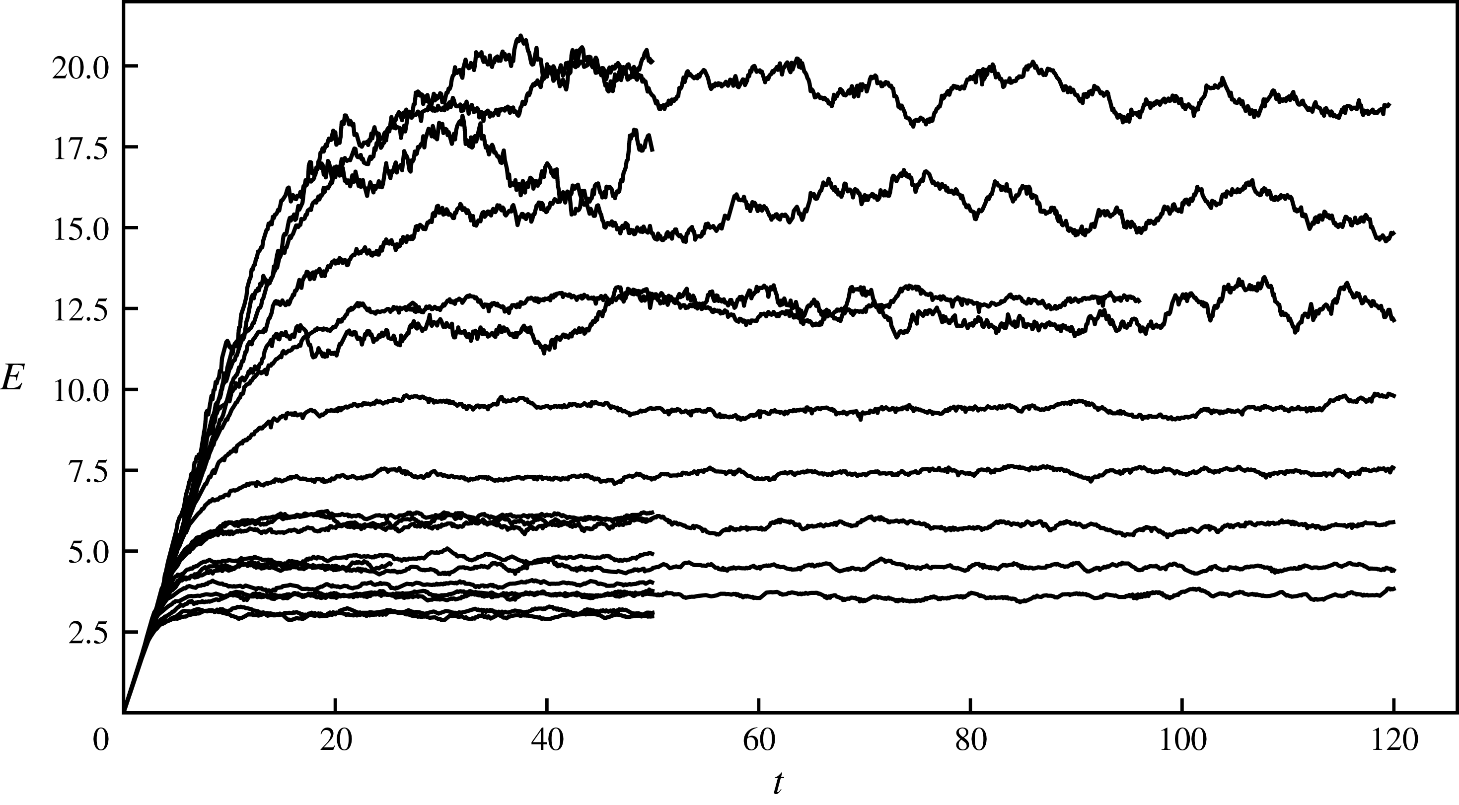
Space averaged energy,
 $E=E_{K}+E_{A}$
, versus time for all simulations.
Parameters for all simulations.
 $n$
, number of nodes in each direction,
 $c$
, wave speed,
 $\unicode[STIX]{x1D708}_{8}$
, hyperviscosity,
 $\unicode[STIX]{x1D716}$
, time averaged mean energy dissipation in the stationary state,
 $k_{d}/k_{f}$
, ratio between dissipation wavenumber and forcing wavenumber,
 $F_{f}$
, Froude number,
 $t_{max}$
, end time of simulation.

(a) Mean energy in the stationary state versus
 $c$
for different resolutions. The lines have slope 0.5, corresponding to
 $E\propto c^{1/2}$
. (b) Normalised mean energy in the stationary state versus resolution
 $n$
for different
 $c$
.

The time evolution of mean energy is shown in figure 1 for all twenty simulations. After an initial period of growth, mean energy is levelling out at different values for different runs. This is not the same picture as we see in simulations of three-dimensional incompressible turbulence or stratified turbulence, where all curves would have levelled out more or less at the same value. We find that mean energy in the stationary state is a function of both
 $c$
(or the Froude number) and resolution
 $n$
and that the functional dependence can be approximately written as
 $$\begin{eqnarray}E\sim \sqrt{\unicode[STIX]{x1D716}L_{f}c}n^{\unicode[STIX]{x1D6FC}}.\end{eqnarray}$$
In figure 2(a), we see
 $E/\sqrt{\unicode[STIX]{x1D716}}$
as a function of
 $c$
for different resolutions
 $n$
. For each resolution the points are approaching a power law
 $C_{n}c^{1/2}$
with increasing values of
 $C_{n}$
for increasing
 $n$
. In figure 2(b) we see
 $E/\sqrt{\unicode[STIX]{x1D716}L_{f}c}$
for different values of
 $c$
. For each
 $c$
the points follow a power law
 $n^{\unicode[STIX]{x1D6FC}}$
, where
 $\unicode[STIX]{x1D6FC}$
is becoming slightly larger with increasing
 $c$
, approaching almost the same value
 $\unicode[STIX]{x1D6FC}\approx 0.33$
for the three highest values of
 $c$
. The relation (3.4) can be reformulated as
 $$\begin{eqnarray}\frac{\unicode[STIX]{x1D716}}{(E^{3/2}/L_{f})}\sim \frac{E^{1/2}}{c}n^{-2\unicode[STIX]{x1D6FC}}.\end{eqnarray}$$
Since the simulations are well resolved the dependence on resolution should not be interpreted as consequence of the numerics but rather as a Reynolds number effect, although it is not hundred per cent clear how a Reynolds number should be defined in our case. We may note, however, that
 $n\sim L_{f}/\unicode[STIX]{x1D6FF}x$
and in the case of Navier–Stokes viscosity we should have
 $\unicode[STIX]{x1D6FF}x\propto \unicode[STIX]{x1D708}$
, according to (2.37). Therefore,
 $n$
may be substituted by a Reynolds number. The normalised energy dissipation on the left-hand side of (3.5) will thus go to zero in the limit of large Reynolds number. This is very different from three-dimensional turbulence where there is a local Richardson–Kolmogorov cascade, in which energy is successively transferred from large to small scales of motion. That the cascade is local means that eddies of a particular scale are not directly influenced by eddies of widely different scales. As a consequence, the normalised dissipation is of the order of unity independent of Reynolds number (Tennekes & Lumley Reference Tennekes and Lumley1972; Pope Reference Pope2000). A review of the experimental evidence and theoretical implications of this fundamental law of Kolmogorov turbulence is given by Vassilicos (Reference Vassilicos2015). Our result (3.5) suggests that SW wave turbulence does not fit into the paradigm of a local Richardson–Kolmogorov cascade. Moreover, it is not only in the limit of large Reynolds number the normalised dissipation will go to zero but also in the limit of strong stratification,
 $E^{1/2}/c\rightarrow 0$
. This is different from three-dimensional stratified turbulence where the ratio on the left-hand side of (3.5) is of the order of unity in the limit of strong stratification (Lindborg Reference Lindborg2006; Brethouwer et al.
Reference Brethouwer, Billant, Lindborg and Chomaz2007).
That the energy transfer is not local in a system where the agent of dissipation is wave breaking or shock formation may be expected. According to the theory of ocean waves by Phillips (Reference Phillips1965), ‘wave interactions are usually incapable of transferring energy from a given wavenumber band as rapidly as it is supplied by the wind’. Instead, energy is fed into each wave mode by the wind field and sucked out from the same mode in ‘intermittent patches of foaming’ or ‘white horses’. This may be a too simplified picture of SW water turbulence, since a broad band energy spectrum develops between the forcing and the dissipation wavenumbers. Nevertheless, shock formation suggests that there is a considerable direct energy transfer from large to very small wavelengths, without any intermediate steps.
The ‘four-fifths law’ for the third-order structure function of Kolmogorov turbulence is often derived using the assumption of a local cascade (Vassilicos Reference Vassilicos2015) or the assumption that dissipation stays finite in the limit of large Reynolds number (Frisch Reference Frisch1995). As we just discussed, these assumptions seem to be violated in the case of SW wave turbulence. Nevertheless, the analogous law (2.25) is satisfied with a high degree of accuracy in our simulations. In figure 3 we see the spectral energy flux from run W7 to the left and the third-order structure function to the right. There is a broad constant flux range with equipartition between KE and APE flux and an almost equally broad range where (2.25) is satisfied, with equipartition between the two third-order structure functions associated with KE and APE. The assumptions of a local cascade and finite dissipation do not seem to be necessary in order for the third-order structure function law (2.25) to be valid.
(a) Time averaged normalised spectral energy fluxes versus
 $k/k_{f}$
. (b) Time averaged normalised third-order structure functions versus
 $r/L_{f}$
. From run W7.

Frequency spectra of KE and APE for different
 $k=|\boldsymbol{k}|$
, from run W7. The spectra are plotted as functions of
 $\unicode[STIX]{x1D714}/\unicode[STIX]{x1D714}_{l}$
, where
 $\unicode[STIX]{x1D714}_{l}=ck$
. From top to bottom:
 $k/\unicode[STIX]{x1D6FF}k=12$
, 27, 62, 143, 327 and 746.

The equipartition of the KE and APE spectral fluxes suggests that the flow to leading order may be described as a collection of linear gravity waves with energy equipartition in each mode. To investigate this further we have collected time series of the flow variables from Fourier modes whose magnitudes fall within certain shells,
 $|\boldsymbol{k}|\in [k-\unicode[STIX]{x1D6FF}k/2,k+\unicode[STIX]{x1D6FF}k/2]$
, and computed temporal power law spectra from these time series and averaged over all wavenumbers in each shell. In other words, we have computed KE and APE frequency spectra corresponding to different magnitudes of modes. Figure 4 presents such spectra plotted as functions of the normalised frequency
 $\unicode[STIX]{x1D714}/\unicode[STIX]{x1D714}_{l}$
, where
 $\unicode[STIX]{x1D714}_{l}=ck$
is the linear wave frequency. The spectra are strongly dominated by peaks at
 $\unicode[STIX]{x1D714}=\unicode[STIX]{x1D714}_{l}$
. As can be seen, there is equipartition between KE and APE in each shell. Although the widening of the peaks around the linear frequency most likely is an effect of nonlinearities, we can quite safely conclude that the time evolution of the flow variables in each Fourier mode to leading order can be described as a linear wave.
(a,c) Divergence
 $\unicode[STIX]{x1D735}\boldsymbol{\cdot }\boldsymbol{u}$
. (b,d) Velocity component in the
 $y$
-direction:
 $u_{y}$
. (a,b) Run W6. (c,d) Run W17.

Visualisations of the flow field give a completely different picture from what may be expected from a collection of linear gravity waves. They are totally dominated by the appearance of shock waves. In figure 5 we see the divergence,
 $\unicode[STIX]{x1D735}\boldsymbol{\cdot }\boldsymbol{u}$
, to the left and the velocity component in the
 $y$
-direction,
 $u_{y}$
, to the right. Note that the total area of the computational domain is sixteen times larger than the area of the outcuts shown in the figures, since the side of the figures is
 $3L_{f}$
, while the side of the computational domain is
 $12L_{f}$
. The two figures at the top are from run W6 while the two figures at the bottom are from run W17. The difference between the two runs is that
 $c$
is larger by a factor of 20 in W17 as compared to W6. To the left we see the shocks displayed as elongated bands of negative divergence. That the divergence is negative at the shocks can be understood from the fact that the velocity component perpendicular to the shock always has a negative jump in the direction of shock propagation. Apparently, the mean distance between the shocks is considerably smaller in run W17 with the larger value of
 $c$
compared to run
 $W6$
with the smaller value of
 $c$
. The shocks are also visible in the figures to right where
 $u_{y}$
is displayed. It may be interesting to note that the shocks along the
 $x$
-axis appear as extra sharp in this plot, since there is a strong jump of
 $u_{y}$
over these shocks, while the shocks along the
 $y$
-axis are hardly visible, since there is no jump of
 $u_{y}$
over these. In the two figures to the right we see a variation of the flow field over the length scale
 $L_{f}$
which is not seen in the two figures to the left. This variation is evidently a footprint of the random forcing. Although the forcing length scale
 $L_{f}$
is the same in the two simulations the mean distance,
 $d$
, between the shocks is much smaller in run
 $W17$
than in run
 $W6$
, which may come as a surprise. Another interesting observation is that the shocks in run W17 (lower figures) appear to have smaller curvature on average than the shocks in run W6 (upper figures). In both runs, the shocks are weak in the sense that the Mach number is close to unity and the interaction between the shocks should therefore be weak (see Apazidis & Eliasson Reference Apazidis and Eliasson2018). However, as measured by the Mach number (2.42), the shocks are much weaker in run W17, where
 $c$
is larger by a factor of 20 as compared to run W6 and
 $d$
also is smaller. The shock interaction should therefore be weaker in run W17, which may explain the observation that the curvature of the shocks is smaller in run W17 than in run W6. We have calculated the mean distance,
 $d$
, between the shocks by counting the number of negative spikes of the divergence along two hundred lines parallel to the
 $x$
-axis and equally many parallel to the
 $y$
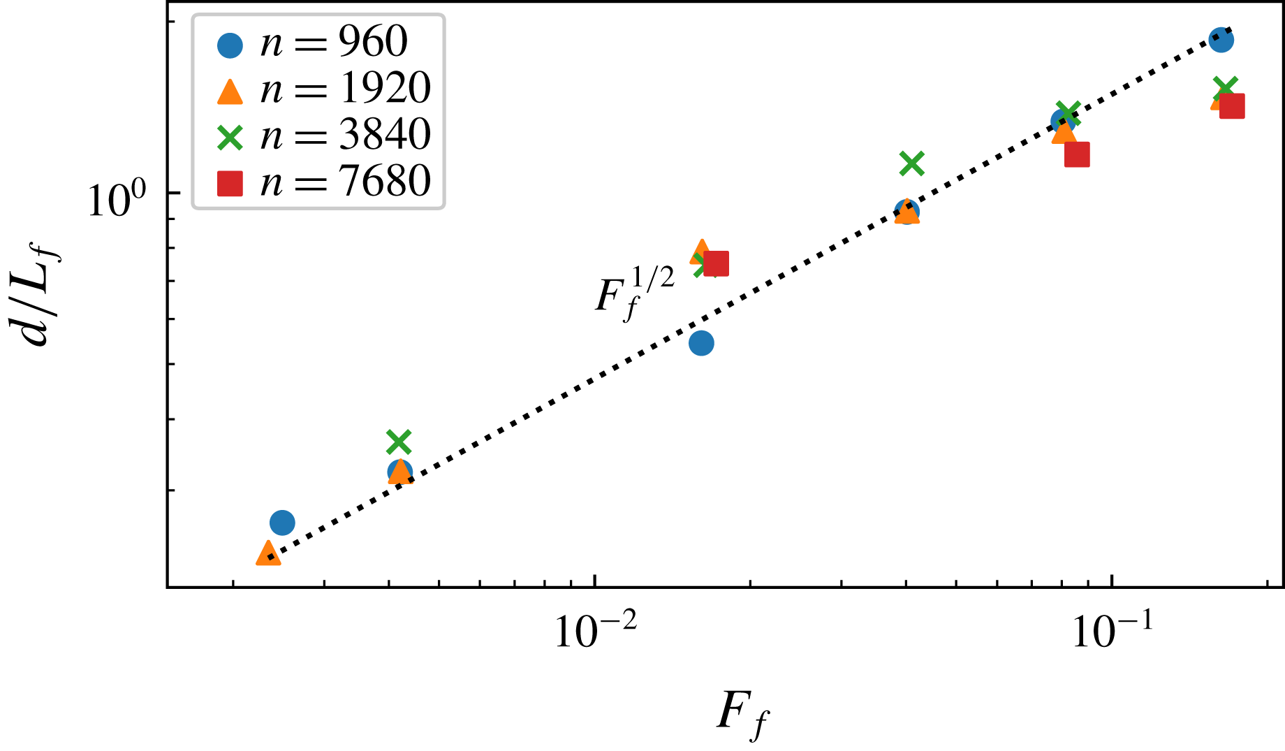
-axis and then divided total length of all the lines by the number of spikes. Generally, we found that
 $d\propto c^{-1/2}$
, or
 $$\begin{eqnarray}d\sim L_{f}F_{f}^{1/2},\end{eqnarray}$$
independent of resolution
 $n$
. In figure 6 we have plotted
 $d/L_{f}$
versus Froude number for all twenty runs. As can be seen, the points follow the
 $F_{f}^{1/2}$
-curve quite well, although there seems to be a slight systematic deviation at the highest
 $F_{f}$
.
Mean distance between the shocks as function of Froude number.
We will now present the results for the structure functions. Substituting (3.6) into (2.33) we find that the structure functions are expected to scale as
 $$\begin{eqnarray}\langle |\unicode[STIX]{x1D6FF}u|^{p}\rangle \sim \langle (c|\unicode[STIX]{x1D6FF}h|)^{p}\rangle \sim (L_{f}F_{f}^{1/2})^{p/3-1}\unicode[STIX]{x1D716}^{p/3}r,\end{eqnarray}$$
for separation distances that fulfil the condition
 $\unicode[STIX]{x1D6FF}x\ll r\ll d$
. The scaling (3.7) is expected to become better and better fulfilled with decreasing
 $c$
(or increasing
 $F_{f}$
). According to (3.6)
 $d$
is increasing with
 $F_{f}$
, and the scaling range is therefore becoming wider for decreasing
 $c$
, if
 $\unicode[STIX]{x1D6FF}x$
or the resolution is kept constant. The scaling (3.7) is also expected to become better and better fulfilled with increased resolution
 $n$
, since
 $\unicode[STIX]{x1D6FF}x$
is decreasing with increasing
 $n$
.
From top to bottom: second-, fourth- and sixth-order compensated and normalised longitudinal structure functions. (a,c,e) Runs with
 $n=3840$
; W3, W7, W11, W14 and W18. (b,d,f) Runs with
 $n=7860$
; W4, W8 and W15.

Ratio of the structure functions
 $R_{p}(r)=\langle |\unicode[STIX]{x1D6FF}u_{L}|^{p}\rangle /\langle |\unicode[STIX]{x1D6FF}u_{T}|^{p}\rangle$
from run W8, for
 $p=2$
, 3, 4, 5, 6. The dotted straight lines indicate the values predicted by (2.31):
 $R_{2}=2$
,
 $R_{3}=3\unicode[STIX]{x03C0}/4$
,
 $R_{4}=8/3$
,
 $R_{5}=15\unicode[STIX]{x03C0}/16$
and
 $R_{6}=16/5$
.

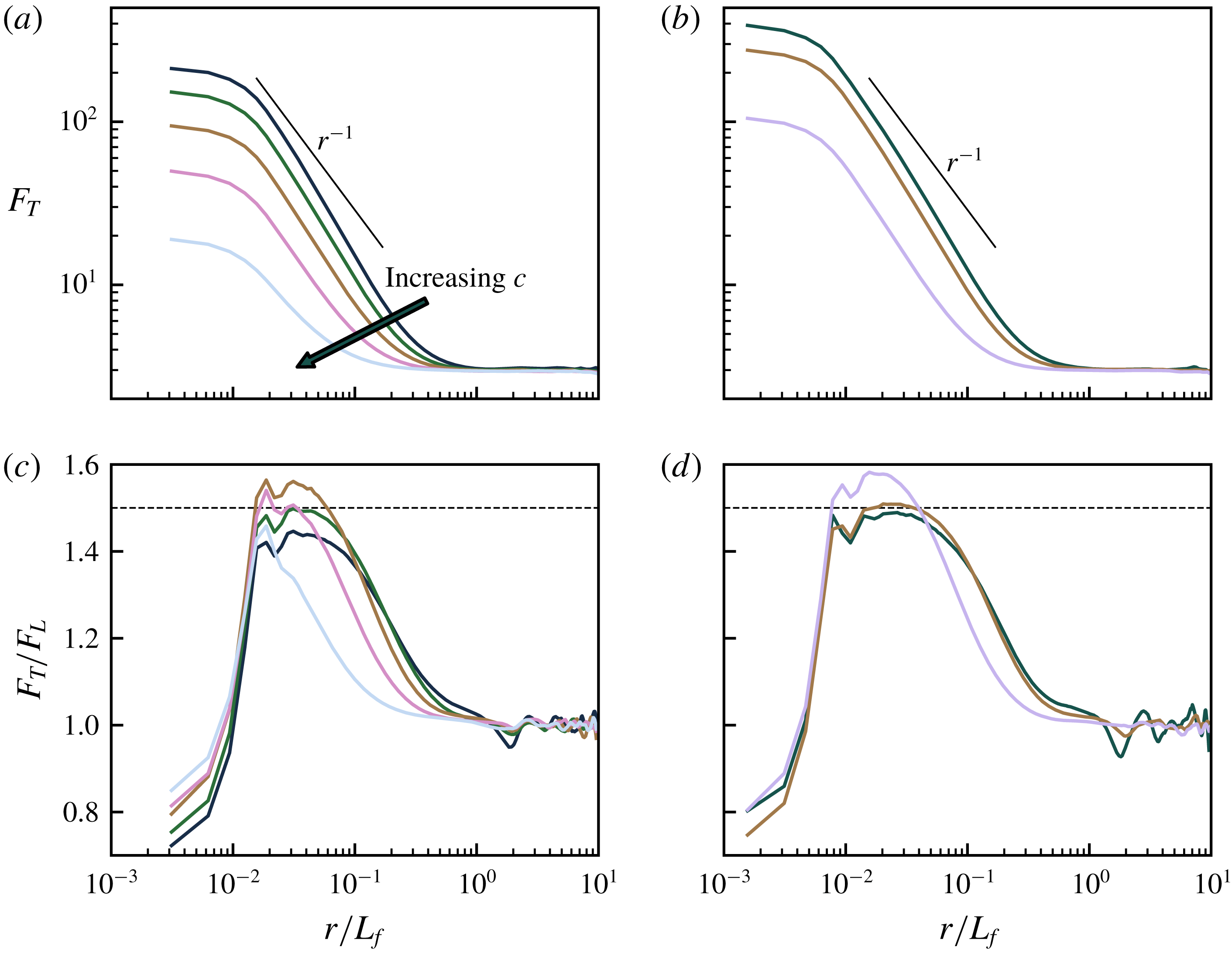
(a,b) Flatness factor of transverse velocity increments. (c,d) Ratio between transverse and longitudinal flatness factors. (a,c) Runs with
 $n=3840$
; W3, W7, W11, W14 and W18. (b,d) Runs with
 $n=7860$
; W4, W8 and W15. The dotted straight lines indicate the value 1.5 predicted by the shock model.
As expected, we have found that the displacement structure functions scale exactly in the same way as the velocity structure functions, and for this reason we only plot velocity structure functions. In figure 7 we see the compensated and normalised second-, fourth- and sixth-order longitudinal structure functions from the five simulations with
 $n=3840$
to the left and the three simulations with
 $n=7860$
to the right. At small separation,
 $r<\unicode[STIX]{x1D6FF}x$
, the structure functions have the dependence
 ${\sim}r^{p}$
, which is characteristic of a smooth velocity field, indicating that the shocks are reasonably well resolved. There is a small bump around the shock width,
 $r\approx \unicode[STIX]{x1D6FF}x$
, and at
 $r>\unicode[STIX]{x1D6FF}x$
, there is a range where the compensated structure functions are flat, or almost flat. As expected, this range is becoming broader for smaller
 $c$
(or larger
 $F_{f}$
). The range is also broader in the higher resolution runs to the right as compared to the lower resolution simulations to the left. There is clearly a better collapse of the curves for the sixth-order structure functions compared to the second-order structure functions. This is not surprising, since the shock contribution to the structure functions should become increasingly dominant with increasing order. Plots of the transverse structure functions are very similar to the plots of the longitudinal structure functions, with the difference that the transverse structure functions are somewhat smoother at
 $r\approx \unicode[STIX]{x1D6FF}x$
. In figure 8 we see the ratio
 $R_{p}(r)=\langle |\unicode[STIX]{x1D6FF}u_{L}|^{p}\rangle /\langle |\unicode[STIX]{x1D6FF}u_{T}|^{p}\rangle$
for
 $p=2$
, 3, 4, 5, 6 from run W8, together with dotted straight lines, indicating the values predicted by (2.31). As can be seen, there is a quite good agreement with the predicted values in a limited range of separations,
 $r>\unicode[STIX]{x1D6FF}x$
. Somewhat unexpectedly, the range in which there is a good agreement becomes more narrow with increasing
 $p$
, an observation that we cannot explain. It may also be noted that
 $R_{2}\rightarrow 3$
in the limit of small
 $r$
, which is the theoretical single point limit for an irrotational isotropic field. In figure 9 we see the flatness factor,
 $F_{T}$
, of the transverse structure functions at the top and the ratio,
 $F_{T}/F_{L}$
, at the bottom. The figures to the left show the results from the five simulations with
 $n=3840$
and the figures to the right show the results from the three simulations with
 $n=7860$
. The flatness factor shows increasingly large values for decreasing
 $r$
with a dependence that is rather close to but somewhat steeper than
 $r^{-1}$
. At small
 $r$
the curves are levelling out at very large values. For
 $n=7869$
and
 $c=10$
we see that
 $F_{T}\approx 400$
at small
 $r$
. The degree to which the flatness factor is increasing with decreasing scale is by some authors defined as the most appropriate measure of spatial intermittency (see for example Frisch Reference Frisch1995). If this measure is used, SW wave turbulence is, indeed, extremely intermittent. In the two figures at the bottom we see that
 $F_{T}/F_{L}\approx 1.5$
in a limited range of separations,
 $r>\unicode[STIX]{x1D6FF}x$
, which is becoming somewhat broader as
 $c$
is increasing and is also somewhat broader in the higher resolution runs shown to the right as compared to the lower resolution runs shown to the left. This is in accordance with the shock model predictions (2.35) and (2.36).
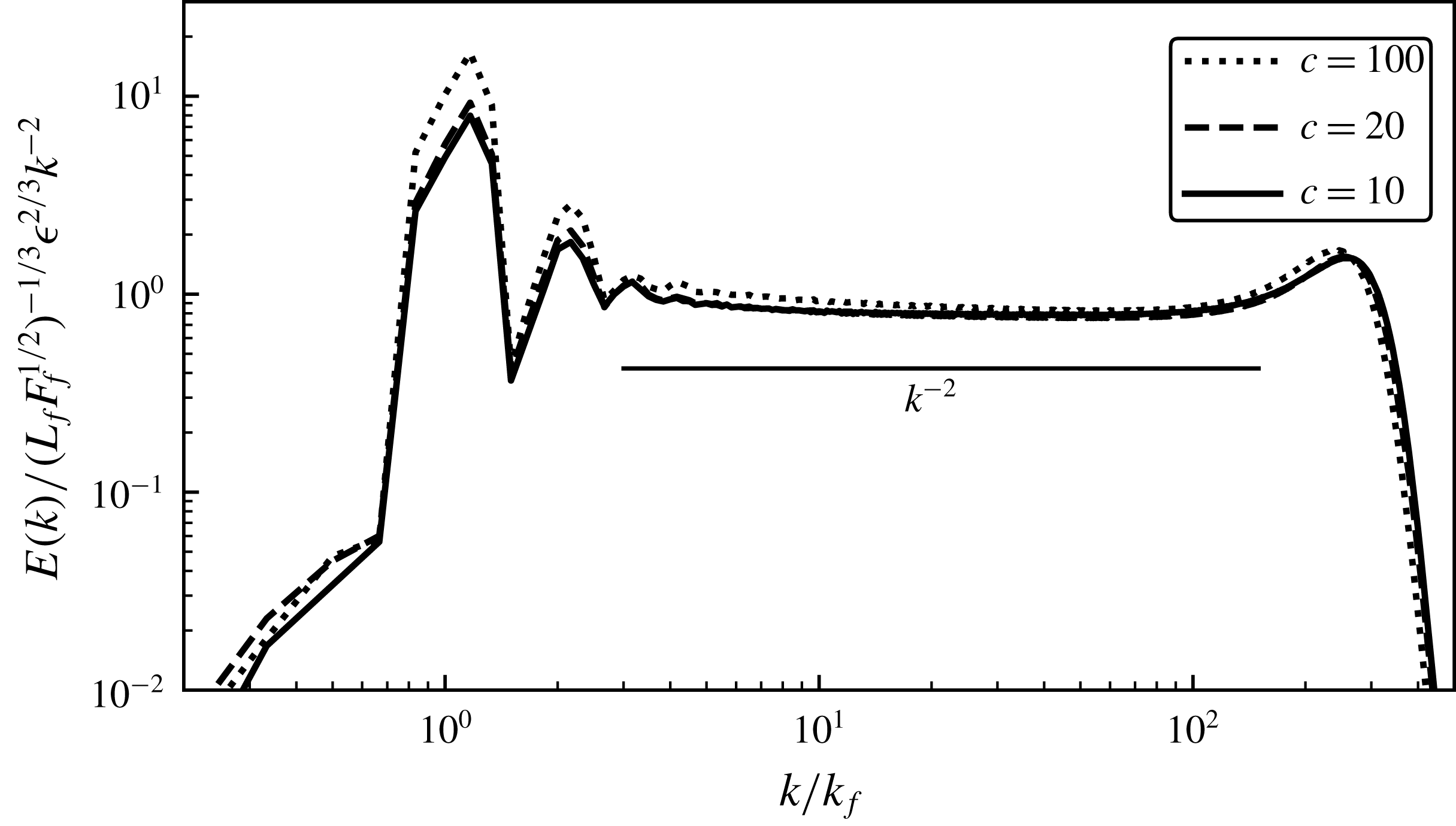
Time averaged compensated and normalised energy spectra from runs with
 $n=7680$
: W4, W8 and W15.
Time averaged normalised dissipation spectra. (a) Constant
 $c=20$
and varying
 $n$
, runs W5, W6, W7 and W8. (b) Constant
 $n=1920$
and varying
 $c$
, runs W2, W6, W10, W13, W17 and W20. The vertical lines indicate the wavenumbers of the maxima.
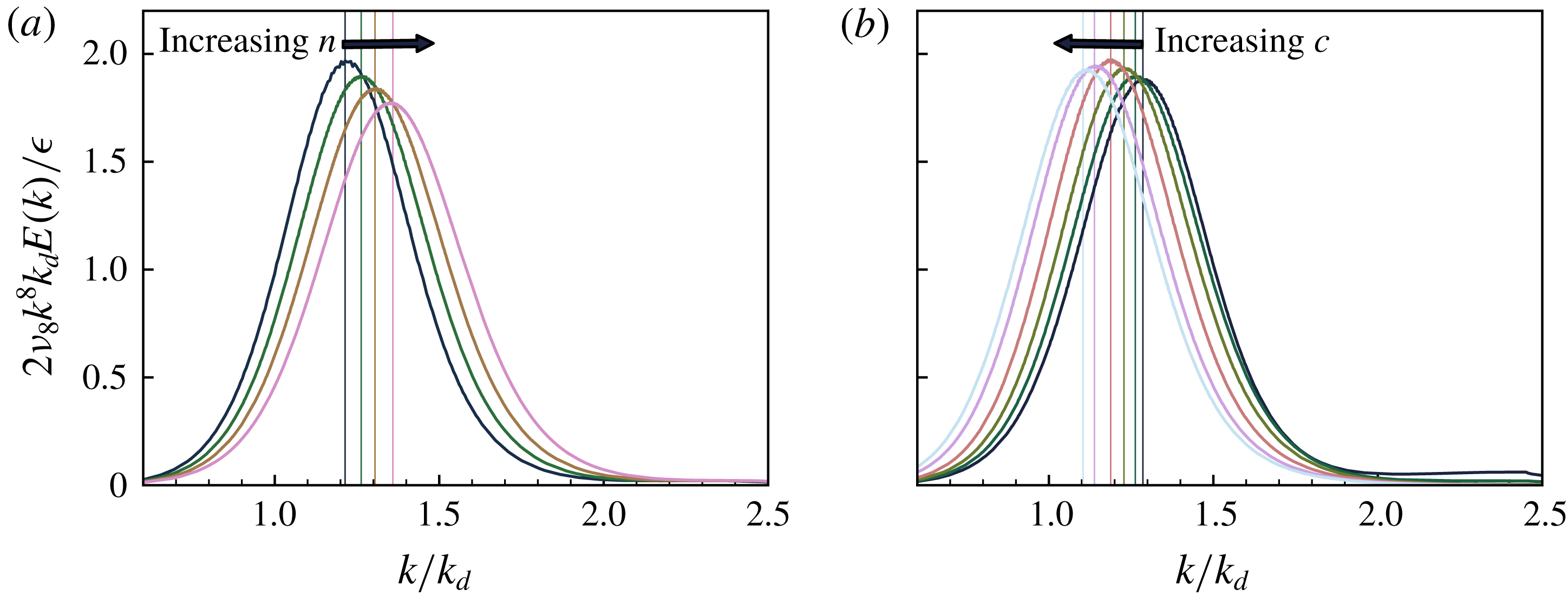
Finally, we present energy and dissipation spectra. As expected, we found that APE and KE spectra were almost identical, Therefore, we only plot the total spectra. In figure 10 we see compensated and normalised energy spectra from the three highest resolution runs. The compensated spectra are almost flat in a broad range. At the high wavenumber end the compensated spectra show a ‘bottleneck’, which we interpret as a signature of the shocks. The
 $k^{-2}$
-dependence and the associated scaling predicted by (2.34) are very well satisfied in a limited range of high wavenumbers close to the bottleneck. At smaller wavenumbers the spectra are becoming somewhat steeper than
 $k^{-2}$
and the spectrum from the run with largest
 $c$
does not collapse perfectly onto the other two spectra. In figure 11 we see normalised dissipation spectra for fixed
 $c=20$
and different
 $n$
to the left, and fixed
 $n=1920$
and different
 $c$
to the right. First, we note that the spectra go to zero quite nicely for large
 $k$
, indicating that the shock width
 $\unicode[STIX]{x1D6FF}x$
is well resolved. Second, we note that there is a slight shift of the maximum in both figures, even though we have normalised the wavenumber by
 $k_{d}=1/\unicode[STIX]{x1D702}_{8}$
. These shifts may be explained by the estimate (3.3) predicting that
 $\unicode[STIX]{x1D6FF}x$
should vary slightly with
 $d$
. If the maximum of the dissipation spectra is associated with
 $\unicode[STIX]{x1D6FF}x$
, there should be a shift of the maximum to the right with increasing
 $n$
and to the left with increasing
 $c$
, since
 $d\propto c^{-1/2}$
. The ratio between the maximum and the minimum
 $n$
in the left figure is equal to 8 and according to (3.3) the corresponding ratio between the wavenumbers at which the maxima are observed should be
 $8^{1/21}\approx 1.1$
, which is exactly the value we observe. The ratio between the maximum and minimum
 $c$
in the right figure is equal to 70. Assuming that
 $d\propto c^{-1/2}$
the ratio between the wavenumbers at which the maxima are observed should be
 $70^{1/42}\approx 1.1$
, while the observed ratio is equal to 1.16. In the latter case, there is no exact quantitative agreement between the predicted trend and the numerical results.
4 Conclusions and discussion
We have carried out a theoretical and numerical investigation of SW wave turbulence. First, we derived the SW analogue (2.25) of the ‘four-fifths’ law of Kolmogorov turbulence. Using this relation and straightforward statistical and geometrical arguments we developed a simple shock model predicting that the shock amplitude scales as
 $(\unicode[STIX]{x1D716}d)^{1/3}$
, where
 $d$
is the mean distance between the shocks, and that the
 $p$
th-order structure function above a certain minimum will scale as
 $(\unicode[STIX]{x1D716}d)^{p/3}r/d$
. Then, we carried out a series of forced-dissipative simulations, varying the Froude number and the resolution. In all simulations, a statistically stationary state was reached and in all simulations we observed shocks. The flow variables in each Fourier mode were found to evolve in accordance with linear wave dynamics, with equipartition between APE and KE over a period. The third-order structure function relation was fulfilled with a high degree of accuracy. From the simulations we made two interesting observations that fall outside the predictive scope of the model. The first observation was that mean energy in the stationary state approximately scales as (3.4), suggesting that the normalised dissipation (3.5) will go to zero both in the limit of small viscosity and large wave speed. A similar observation was made when we used a second-order diffusion operator instead of hyper diffusion (see appendix A). This is different from three-dimensional Kolmogorov turbulence as well as strongly stratified turbulence, where, in both cases, dissipation is finite in the limit of small viscosity, and in the latter case also is independent of the degree of stratification. This observation suggests that SW wave turbulence does not fit into the paradigm of a local Richardson–Kolmogorov cascade. It remains a theoretical challenge to give a quantitative explanation of the growth of energy with increased Reynolds number. As far as we can see, such an explanation would require a completely novel theoretical development. The second observation we made was that the mean distance between the shocks scales as
 $c^{-1/2}$
, if the other parameters are held constant. As we increased
 $c$
, the shocks were thus becoming denser. Using this observation we tested the shock model by plotting the normalised and compensated structure functions of different orders. Generally we found that there was a quite good agreement between the simulation results and the model predictions, becoming better with decreasing wave speed and increasing resolution.
Combining the model and the observations we can get a quite good picture of the dynamics in the limit of weak nonlinearities,
 $F_{f}\rightarrow 0$
. The picture may become more vivid if we say ‘wave breaking’ where we previously have talked about shock formation, and also say ‘wavelengths’ were we previously have talked about length scales. We identify the longest wavelength,
 $\unicode[STIX]{x1D706}_{l}$
, with the forcing scale
 $L_{f}$
and the breaking wavelength,
 $\unicode[STIX]{x1D706}_{b}$
, with the mean distance,
 $d$
, between the shocks. There are two dynamically different regimes, the short wave regime,
 $[\unicode[STIX]{x1D6FF}x,\unicode[STIX]{x1D706}_{b}]$
, and the long wave regime,
 $[\unicode[STIX]{x1D706}_{b},\unicode[STIX]{x1D706}_{l}]$
. We first consider the latter, whose width scales
 $\unicode[STIX]{x1D706}_{l}/\unicode[STIX]{x1D706}_{b}\sim F_{f}^{-1/2}$
. Identifying the amplitude of the breaking waves with the shock amplitude,
 $(\unicode[STIX]{x1D716}d)^{1/3}$
, we find that the ratio between the amplitude of the longest waves and the breaking waves scales as
 $E^{1/2}/(\unicode[STIX]{x1D716}d)^{1/3}\sim F_{f}^{-5/12}n^{\unicode[STIX]{x1D6FC}/2}$
, where we may substitute
 $n$
with a Reynolds number. Thus, for small
 $F_{f}$
and large Reynolds numbers the longest waves are not directly influenced by wave breaking. The Reynolds number dependence of the amplitude ratio makes it unlikely that a general similarity theory can be easily formulated for this range. Therefore, predictions from weak turbulence theory (for example Zakharov & Sagdeev Reference Zakharov and Sagdeev1970) are not likely to hold for this range, although it is not directly influenced by wave breaking. The exact values of the power law exponents in the argument leading to this conclusion are, of course, not important. As for the short wave regime, the width scales as
 $\unicode[STIX]{x1D706}_{b}/\unicode[STIX]{x1D6FF}x\sim F_{f}^{1/2}$
for fixed
 $\unicode[STIX]{x1D6FF}x$
or fixed Reynolds number. As
 $F_{f}\rightarrow 0$
the range will eventually become so narrow so that breaking will disappear. As argued in appendix A, the condition
 $\unicode[STIX]{x1D706}_{b}\gg \unicode[STIX]{x1D6FF}x$
leads to a wave breaking condition involving both the Reynolds number,
 $Re\equiv \unicode[STIX]{x1D716}^{1/3}L_{f}^{4/3}/\unicode[STIX]{x1D708}$
, and the Froude number. If
 $\unicode[STIX]{x1D706}_{b}\propto F_{f}^{m}$
we obtain the condition
 $Re\,F_{f}^{4m/3}\gg 1$
and in the special case when
 $m=1/2$
, the condition is
 $$\begin{eqnarray}Re\,F_{f}^{2/3}\gg 1.\end{eqnarray}$$
Thus, for a given Reynolds number, no matter how large, wave breaking will be absent provided that
 $F_{f}$
is sufficiently small. On the other hand, if (4.1) not only is a necessary but also a sufficient condition, wave breaking will be present for any given
 $F_{f}$
, no matter how small, provided that
 $Re$
is sufficiently large. The condition (4.1) is analogous to the condition for the presence of turbulence in a stratified fluid, also involving both the Reynolds number and a Froude number (Brethouwer et al.
Reference Brethouwer, Billant, Lindborg and Chomaz2007). The horizontal and vertical length scales of stratified turbulence scale as
 $l_{h}\sim u^{3}/\unicode[STIX]{x1D716}$
and
 $l_{v}\sim u/N$
, respectively, where
 $u$
is a characteristic horizontal velocity and
 $N$
is the Brunt–Väisälä frequency. As stratification becomes stronger (
 $N$
is increasing),
 $l_{v}$
is becoming smaller. However, in order for turbulence to be present
 $l_{v}$
must be much larger than the Kolmogorov scale,
 $\unicode[STIX]{x1D708}^{3/4}/\unicode[STIX]{x1D716}^{1/4}$
, which leads to the condition
 $ReF_{h}^{2}\gg 1$
, where
 $F_{h}=u/(l_{h}N)$
is a Froude number based on the horizontal length scale.
The present study makes some advancement of the understanding of compressible turbulence. Previously, energy flux relations have been derived for a compressible and barotropic fluid by Falkovich, Fouxon & Oz (Reference Falkovich, Fouxon and Oz2010) and Galtier & Banarjee (Reference Galtier and Banarjee2011). Unlike (2.24) these flux relations are not exclusively expressed in terms of third-order structure functions, i.e. third-order moments of increments of flow variables. As is clear from our analysis, in the general case of a compressible and irrotational fluid the KE flux can be expressed in this way. It seems to be more of a specific property that the APE flux also can be expressed in terms of a third-order structure function, a property that the SW system shares with the Boussinesq system with constant Brunt–Väisälä frequency, in which case APE also is quadratic in buoyancy (Augier, Galtier & Billant Reference Augier, Galtier and Billant2012). In this context, a comparison between our analysis and the analysis by Galtier & Banarjee (Reference Galtier and Banarjee2011) of isothermal compressible turbulence is revealing. In the latter case, the pressure is linear in density,
 $p=c_{t}^{2}\unicode[STIX]{x1D70C}$
, where
 $c_{t}$
is the isothermal speed of sound, and the internal energy per unit volume is equal to
 $c_{t}^{2}\unicode[STIX]{x1D70C}\ln (\unicode[STIX]{x1D70C}/\unicode[STIX]{x1D70C}_{0})$
, where
 $\unicode[STIX]{x1D70C}_{0}$
is an ambient reference density. Due to this logarithmic dependence, the internal energy flux is not expressible in terms of a structure function. However, an equation system which is equivalent to the SW equations can be obtained by replacing the pressure term,
 $\unicode[STIX]{x1D70C}^{-1}\unicode[STIX]{x1D735}p=\unicode[STIX]{x1D70C}^{-1}c_{t}^{2}\unicode[STIX]{x1D735}\unicode[STIX]{x1D70C}$
, in the isothermal momentum equation, by
 $\unicode[STIX]{x1D70C}_{0}^{-1}c_{t}^{2}\unicode[STIX]{x1D735}\unicode[STIX]{x1D70C}$
, which may be motivated if density fluctuations are small. The expression for the internal energy per unit volume of the modified system is
 $c_{t}^{2}\unicode[STIX]{x1D70C}^{2}/2\unicode[STIX]{x1D70C}_{0}$
, which is equivalent to the SW potential energy. (To see how the logarithmic and quadratic expressions for the internal energy are related, write
 $\unicode[STIX]{x1D70C}=\unicode[STIX]{x1D70C}_{0}(1+\unicode[STIX]{x1D702})$
, expand in
 $\unicode[STIX]{x1D702}$
and keep terms up to second order:
 $c_{t}^{2}\unicode[STIX]{x1D70C}\ln (\unicode[STIX]{x1D70C}/\unicode[STIX]{x1D70C}_{0})\approx c_{t}^{2}\unicode[STIX]{x1D70C}_{0}(1+\unicode[STIX]{x1D702})(\unicode[STIX]{x1D702}-\unicode[STIX]{x1D702}^{2}/2)\approx c_{t}^{2}\unicode[STIX]{x1D70C}^{2}/2\unicode[STIX]{x1D70C}_{0}-c_{t}^{2}\unicode[STIX]{x1D70C}_{0}/2$
. For small density fluctuations the two expressions only differ by a constant.) As a consequence of this quadratic dependence, the internal energy flux is expressible in terms of a structure function. It may be conjectured that the modified equation system is a good model for isothermal acoustic turbulence and that a flux relation which equivalent to (2.24) also should hold for this case. In the three-dimensional case we then obtain
 $$\begin{eqnarray}\langle \unicode[STIX]{x1D6FF}(\unicode[STIX]{x1D70C}u_{L})|\unicode[STIX]{x1D6FF}\boldsymbol{u}|^{2}\rangle +c_{t}^{2}\langle \unicode[STIX]{x1D6FF}u_{L}(\unicode[STIX]{x1D6FF}\unicode[STIX]{x1D70C})^{2}\rangle /\unicode[STIX]{x1D70C}_{0}=-{\textstyle \frac{8}{3}}\unicode[STIX]{x1D716}r,\end{eqnarray}$$
where
 $\unicode[STIX]{x1D716}$
here is the mean energy dissipation rate per unit volume.
While isothermal acoustic turbulence may have some interesting application for a radiating gas (Stein & Spiegel Reference Stein and Spiegel1967), standard text book acoustics is not isothermal but isentropic. The condition of constant entropy puts us in a dilemma when we analyse an acoustic field as a forced–dissipative system, since dissipation inevitably is associated with entropy production. According to arguments of Kadomtsev & Petviashvili (Reference Kadomtsev and Petviashvili1973), an acoustic field is always dissipated by weak shocks if the Reynolds number is sufficiently large, and this should be true in two as well as in three dimensions. Given the numerical results of the present study such a hypothesis seems reasonable, since shock waves have similar stability properties in two and three dimensions (Liverts & Apazidis Reference Liverts and Apazidis2016; Apazidis & Eliasson Reference Apazidis and Eliasson2018). The shock wave hypothesis offers an elegant way out of the isentropic dilemma, since it implies that entropy production is concentrated at the shocks, while the rest of the field can be treated as isentropic. In a companion paper (Lindborg Reference Lindborg2019), scaling relations for such an acoustic field are derived, using the weak shock relations and the entropy equation. It turns out that these scaling relations are analogous to the relations for shallow water wave turbulence, with the difference that the mean energy dissipation rate,
 $\unicode[STIX]{x1D716}$
, is replaced by
 $\unicode[STIX]{x1D716}+\unicode[STIX]{x1D712}$
, where
 $\unicode[STIX]{x1D712}$
is a quantity associated with entropy production due to heat conduction. If the Prandtl number is of the order of unity,
 $\unicode[STIX]{x1D712}$
is of the same order as
 $\unicode[STIX]{x1D716}$
. The shock amplitude scales as
 $\unicode[STIX]{x0394}u\sim (\unicode[STIX]{x1D716}+\unicode[STIX]{x1D712})^{1/3}d^{1/3}$
, where
 $d$
is the characteristic distance between the shocks and the third-order longitudinal structure function scales as
 $\langle \unicode[STIX]{x1D6FF}u_{L}^{3}\rangle =-C(\unicode[STIX]{x1D716}+\unicode[STIX]{x1D712})r$
, where
 $C$
is a constant of the order of unity, which can be determined exactly in the weak shock limit.
Acoustic turbulence is an example of a wave breaking system where the concepts and methods we have developed to analyse SW water turbulence can be applied in a fruitful way. We believe that there may be other such examples.
Acknowledgements
The authors would like to thank G. Falkovich and S. Nazarenko for fruitful criticism of an early version of the manuscript, S. Galtier for making a check of the final manuscript and three anonymous reviewers for useful comments. Financial support from the Swedish Research Council (VR) is gratefully acknowledged (grant no. D0519101). The simulations were performed on resources provided by the Swedish National Infrastructure for Computing (SNIC) at PDC.
Appendix A. Simulations with Laplacian diffusion
On the request from the reviewers we have carried out a set of simulations using Laplacian diffusion,
 $\unicode[STIX]{x1D708}\unicode[STIX]{x1D6FB}^{2}$
, to check that similar results are obtained in this case as when we use higher-order diffusion
 $\unicode[STIX]{x1D708}_{8}\unicode[STIX]{x1D6FB}^{8}$
. A number of test simulations with resolution
 $n=960$
and
 $c=10$
were first carried out using different values of the viscosity, until we determined a value which was sufficiently large for the shocks to be resolved, but not unnecessarily large. This value was then used for all simulations with
 $n=960$
. For the more highly resolved simulations the viscosity was then set as
 $\unicode[STIX]{x1D708}\propto n^{-1}$
, in accordance with the prediction (2.37) for the shock width. We define the Reynolds number as
 $Re\equiv \unicode[STIX]{x1D716}^{1/3}L_{f}^{4/3}/\unicode[STIX]{x1D708}$
, which is proportional to
 $n$
, since
 $~\unicode[STIX]{x1D708}\propto n^{-1}$
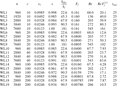
. The simulations are listed in table 2.
Parameters for all the simulations executed with Laplacian viscosity.
 $n$
, number of nodes in each direction,
 $c$
, wave speed,
 $\unicode[STIX]{x1D708}$
, viscosity,
 $\unicode[STIX]{x1D716}$
, time averaged mean energy dissipation in the stationary state,
 $k_{d}/k_{f}$
, ratio between dissipation wavenumber and forcing wavenumber,
 $F_{f}$
, Froude number,
 $Re$
, Reynolds number,
 $t_{max}$
, end time of simulation.
The dynamics of the runs with Laplacian diffusion was similar to the runs with higher-order diffusion. In figure 12 we see mean energy in the stationary state versus
 $c$
to the left and versus
 $n$
to the right. The variation of mean energy with
 $c$
seems to be a little bit weaker for these runs as compared to the runs with hyper diffusion. However, the higher resolution runs are relatively close to approaching the
 $c^{1/2}$
-scaling. The variation of mean energy with resolution, or Reynolds number, is quite similar to what is seen in the corresponding figure 2. For each
 $c$
there is a monotonic increase of mean energy with resolution, and the increase is becoming stronger as
 $c$
is increased, with comparable but not equal values of the exponent
 $\unicode[STIX]{x1D6FC}$
.
(a) Mean energy in the stationary state versus
 $c$
for different resolutions. The lines have slope 0.5, corresponding to
 $E\propto c^{1/2}$
. (b) Normalised mean energy in the stationary state versus resolution
 $n$
for different
 $c$
.

Mean distance between the shocks as function of Froude number.
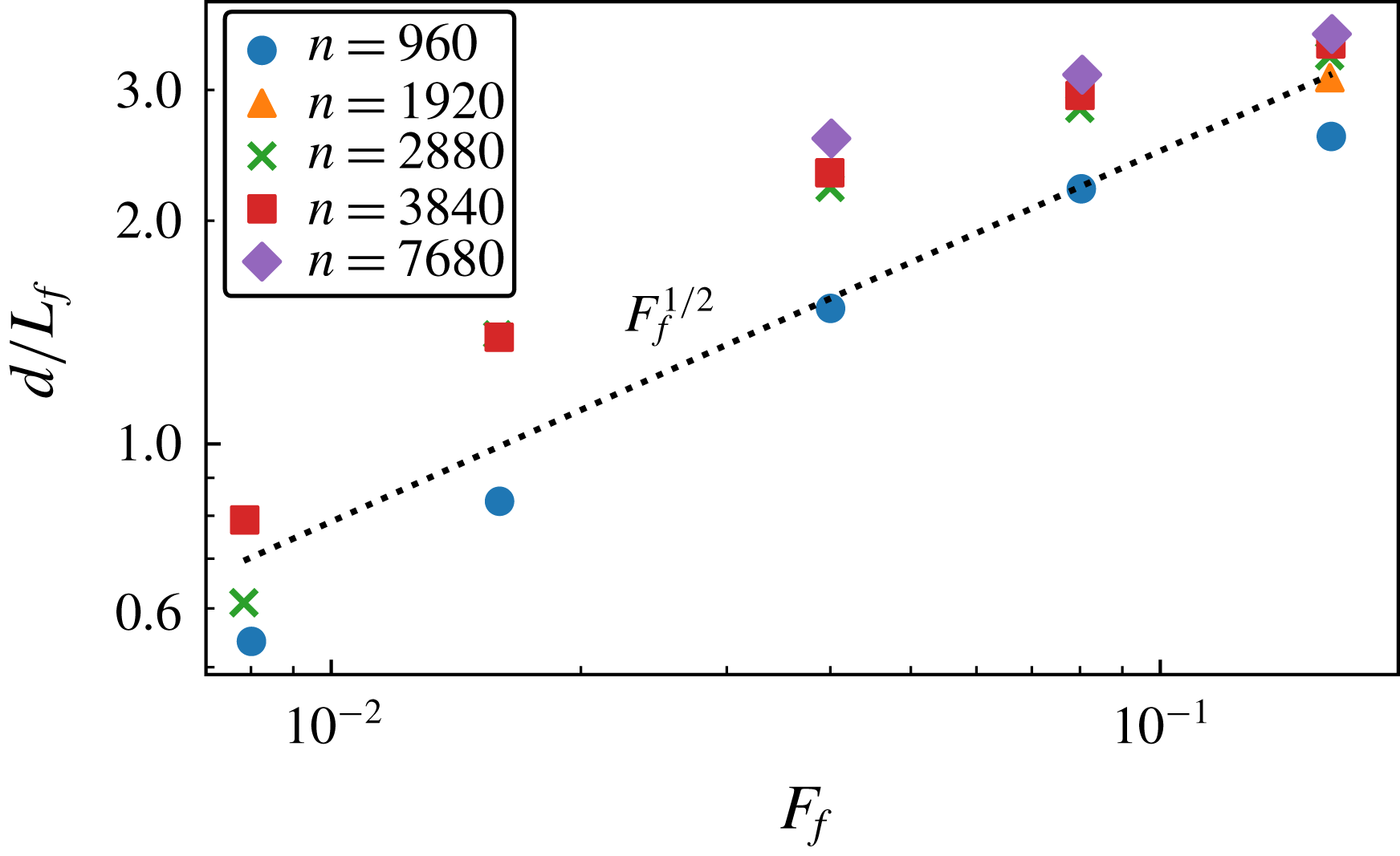
Flatness of divergence
 $\unicode[STIX]{x1D735}\boldsymbol{\cdot }\boldsymbol{u}$
times viscosity
 $\unicode[STIX]{x1D708}$
, versus
 $F_{f}$
. Dotted straight line indicates
 $F_{f}^{2/3}$
.
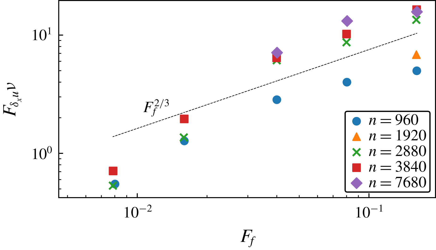
Value of
 $\unicode[STIX]{x1D735}\boldsymbol{\cdot }\boldsymbol{u}$
for four different runs. (a) WL1,
 $Re=68$
,
 $F_{f}=0.16$
; (b) WL3,
 $Re=203$
,
 $F_{f}=0.16$
; (c) WL17,
 $Re=68$
,
 $F_{f}=0.008$
; (d) WL18,
 $Re=199$
,
 $F_{f}=0.008$
.
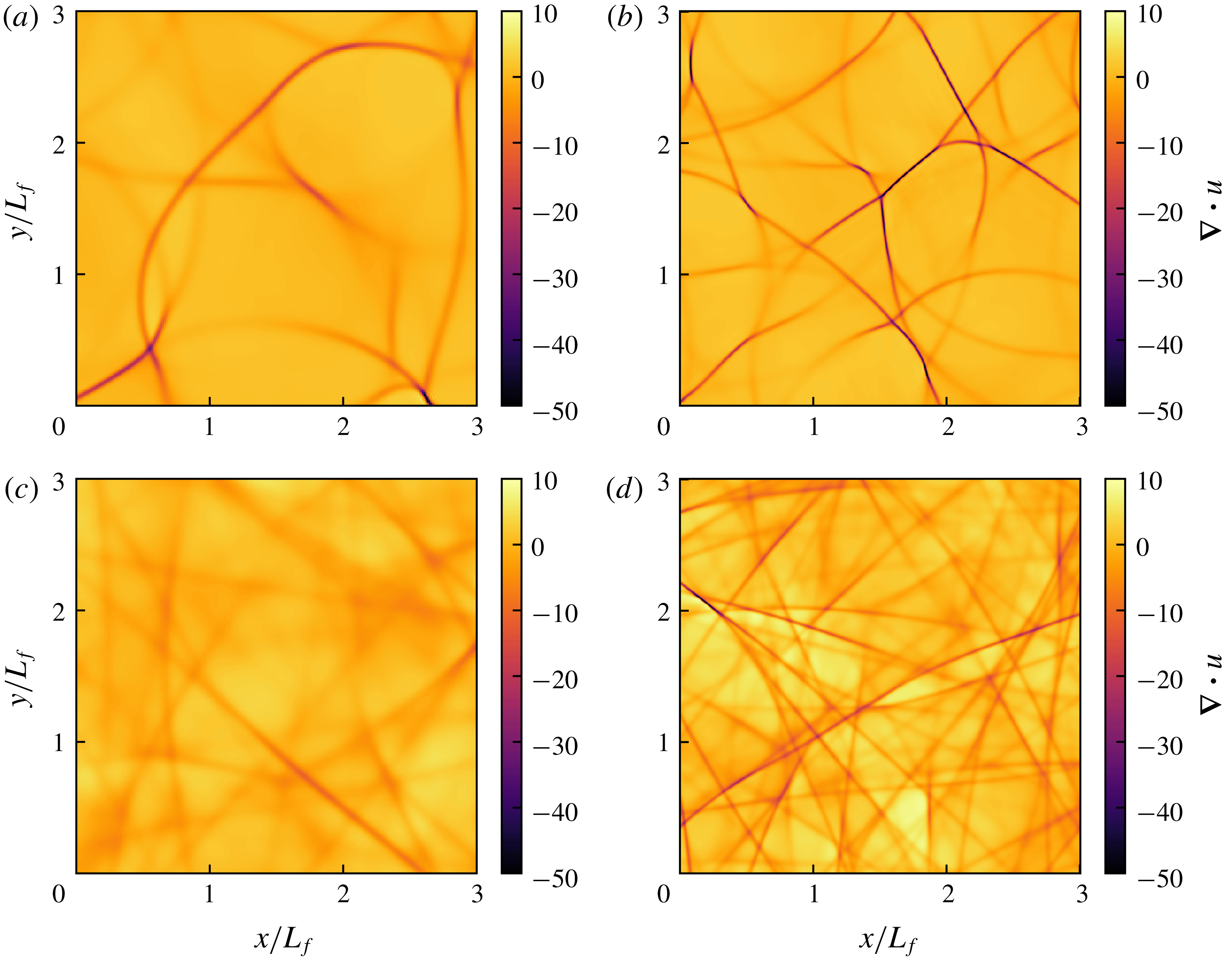
In figure 13 we see the mean distance between the shocks as a function of
 $F_{f}$
, together with a straight line indicating
 $F_{f}^{1/2}$
. As compared to the runs with hyperviscosity there is a larger spread of the points and the
 $F_{f}^{1/2}$
scaling is not as clear. The lower Reynolds number series (
 $Re\approx 70$
blue dots) falls below the higher Reynolds number series. This may be explained by the fact that the shock detection algorithm is much more sensitive to the threshold value which is used for
 $\unicode[STIX]{x1D735}\boldsymbol{\cdot }\boldsymbol{u}$
in these simulations than in the simulations with hyperviscosity. In particular, this is true in the lower Reynolds number runs. In figure 14 we see the flatness of the divergence, multiplied by
 $\unicode[STIX]{x1D708}$
, versus
 $F_{f}$
. According to (2.40) we should have
 $F_{\unicode[STIX]{x2202}u}\unicode[STIX]{x1D708}\propto d^{4/3}$
and if
 $d\propto Fr^{1/2}$
, the points should collapse on a single line,
 $F_{f}^{2/3}$
. For the three largest
 $F_{f}$
, there is a relatively good collapse of the points from the three highest Reynolds numbers series, supporting both the
 $\unicode[STIX]{x1D708}^{-1}$
-scaling and the
 $F_{f}^{2/3}$
-scaling. The lower Reynolds number runs (blue dots) fall below the higher Reynolds number runs, which we interpret as a low Reynolds number effect. The points corresponding to the two lowest values of
 $F_{f}$
fall below the prediction
 $F_{f}^{2/3}$
. This can be explained by the fact that the shocks are on the verge of fading away in these runs. Clearly, a necessary condition for shocks to be present is that the mean distance between them is much larger than their width, that is
 $$\begin{eqnarray}\frac{d}{\unicode[STIX]{x1D6FF}x}\gg 1.\end{eqnarray}$$
Since
 $F_{\unicode[STIX]{x2202}u}\propto d/\unicode[STIX]{x1D6FF}x$
, this means that the flatness of divergence must be much larger than unity. Substituting (2.37) into (A 1) and assuming that (3.6) is valid we can formulate the condition as
 $$\begin{eqnarray}Re\,F_{f}^{2/3}\gg 1.\end{eqnarray}$$
If this condition is not fulfilled the shocks will fade away. In figure 15 we have plotted the divergence for four different runs with different
 $Re$
and
 $F_{f}$
. It should be pointed out again, that the area of the computational domain is sixteen times larger than area of the outcuts shown in the figures. (a,b) are from simulations with
 $F_{f}=0.16$
but different
 $Re$
(
 $Re=68$
(a) and
 $Re=203$
(b)). As can be seen, the shocks are wider in the lower Reynolds number run (a) than in the higher Reynolds number run (b), as expected. (c) is from a simulation with the same
 $Re$
as in (a), but with a much smaller
 $F_{f}$
. In this simulation we have
 $Re\,F_{f}^{2/3}=2.7$
, so the condition (A 2) is not fulfilled, and the shocks have almost faded away. (d) is from a simulation with the same
 $F_{f}$
as in (c), but with a higher
 $Re=199$
. Here,
 $Re\,F_{f}^{2/3}=7.8$
and the shocks are clearly discernible. Comparing (b) and (d) with each other, they have approximately the same
 $Re$
, while the lower one has a considerably lower
 $F_{f}$
. In this run the shocks are denser and straighter as compared to the higher
 $F_{f}$
-run.


 Open access

