





1. Introduction
Over recent decades, as knowledge of automotive aerodynamics has grown, the design of most vehicle classes, such as cars, has moved in favour of more streamlined, aerodynamically efficient bodies. While this has occurred to some extent for the fronts of trucks, given practical and regulatory limitations of the rear of truck exteriors, such as the need for rectangular trailers to maximise storage capacity, traditional streamlining is often not practical. Active flow control is an attractive alternative that retains the potential to reduce drag while maintaining the required shape of the vehicle.
Due to the relatively complex shapes of the frontal section of trucks and the potential differences between makes and models, it is generally beneficial to consider simplified, reduced-feature models with the aim of gaining more generalised, widely applicable knowledge. These models tend to consist of a square or rectangular base extruded upstream, with a frontal surface incorporating curved edges to some degree, such as the Ahmed body (Ahmed et al. Reference Ahmed, Ramm and Faltin1984) or the ground transportation system (GTS) model. However, even these simplified geometries can have a relatively complex wake dynamics (Grandemange et al. Reference Grandemange, Gohlke and Cadot2013), leading researchers to simplify the geometry further by considering a two-dimensional cross-section of these geometries (e.g. Pastoor et al. Reference Pastoor, Henning, Noack, King and Tadmor2008; Parkin et al. Reference Parkin, Thompson and Sheridan2013).
Pastoor et al. (Reference Pastoor, Henning, Noack, King and Tadmor2008) examined wake control and drag reduction for a two-dimensional (2-D) reverse-D-shaped cylinder (based on an Ahmed-body cross-section) using open- and closed-loop active control. They found that periodic control with in-phase zero-net-mass-flux jets angled outwards at 45
 $^\circ$
at the rear corners could maintain wake symmetry of the separating shear layers, effectively increasing the formation length (or mean recirculation bubble size –
 $L_{wake}$
) and decreasing drag by up to 15 %. Using active control based on sensing the behaviour of the opposite shear layer to drive the perturbation of the other shear layer achieved similar gains, but with lower energy input. A similar investigation based on large eddy simulations but only looking at open-loop control was conducted by Parkin et al. (Reference Parkin, Thompson and Sheridan2013). They used vertical jets at the top and bottom surfaces and horizontal jets on the rear surface, with the jets positioned adjacent to the corners. Again, the roll-up of the separating shear layers could be symmetrised, leading to formation length extension and drag reduction. In this case, the optimum forcing frequency was slightly lower (
 $\textit{St} = 0.11$
) than that found by Pastoor et al. (Reference Pastoor, Henning, Noack, King and Tadmor2008) (
 $\textit{St}=0.15$
). These frequencies are approximately half of the shedding frequency.
Parezanović & Cadot (Reference Parezanović and Cadot2012) used a small control cylinder to influence the wake formation from a reverse-D-shaped cylinder. They generated a sensitivity map showing how cylinder position affected the wake flow and the effect on drag. Their smallest control cylinder has been chosen to have a diameter similar to the shear-layer thickness – thereby causing a forcing at the shear-layer frequency rather than the natural shedding frequency. This follows on from the classical study of Strykowski & Sreenivasan (Reference Strykowski and Sreenivasan1990) on experimental control of a circular cylinder wake and theoretical analysis of wake sensitivity and mode suppression of Giannetti & Luchini (Reference Giannetti and Luchini2007) and Marquet et al. (Reference Marquet, Sipp and Jacquin2008) for laminar flow. Higher forcing frequencies deflect and stabilise the separating shear layers, reducing turbulent entrainment, which leads to lower drag. For an axisymmetric bullet-shaped body, Oxlade et al. (Reference Oxlade, Morrison, Qubain and Rigas2015) found that high-frequency oscillatory jets placed around the rear surface close to the separation point could be used to increase the base pressure by up to 35 %, possibly limited by experimental constraints.
Many of these studies tend to concentrate on standalone geometries in the free stream without considering the influence of the ground, which is an aspect that the present study includes.
Parkin et al. (Reference Parkin, Sheridan and Thompson2015) found that including a moving ground plane close to a 2-D, square-backed Ahmed body diminished the effect of the periodic open-loop control method used by Pastoor et al. (Reference Pastoor, Henning, Noack, King and Tadmor2008) and Parkin et al. (Reference Parkin, Thompson and Sheridan2013). That control mechanism targeted the Kármán-like shedding in the wake of the body by attempting to force the vortices from each shear layer to be shed synchronously, thereby resulting in the cross-annihilation of the vortices. The ground plane was found to limit the formation of coherent large-scale vortical structures in the natural flow, and as a result, nullified the effectiveness of that control mechanism. However, Easanesan et al. (Reference Easanesan, Burton and Thompson2020) found that the significant flow separation over the Ahmed-body nose contributed to the reduction in coherent shedding and that more streamlined nose shapes, such as a half-ellipse, continued to produce coherent, albeit asymmetrical, large-scale vortices in the presence of a ground plane, which may remain a valid target for flow control.
For 3-D square-backed bodies, Grandemange et al. (Reference Grandemange, Gohlke and Cadot2013) found that vortex shedding stemming from the interactions of opposing top and bottom shear layers was still present, but weaker. This has implications for methods targeting vortex shedding. For example, Whiteman (Reference Whiteman2016) found that constant suction on the top rear edge and blowing at the rear centre on a 2-D square-backed Ahmed body resulted in the cessation of vortex shedding and large reductions in drag, albeit in planar, 2-D unsteady Reynolds-averaged Navier–Stokes simulations. However, this behaviour did not extend to 3-D geometries.
In this context, instead of vortex shedding, it is useful to consider other avenues for reducing wake entrainment. These efforts have often focused on the manipulation of the bulk wake flow topology, particularly the wake length and aspect ratio. A common approach to this is to divert the separating shear layer in some manner. For example, some success in reducing the drag was seen by Englar (Reference Englar2001), who used constant jets and geometric modifications to generate jet turning angles on a GTS model. In that case, the geometric modifications may have independently contributed to the drag reduction by providing a ‘boat-tailing’ effect. A similar approach was used by Eichinger (Reference Eichinger2012), except with angled jets and no geometric modifications. They found that an angle of 45
 $^\circ$
resulted in the greatest reduction in drag. A similar finding was also made by Rouméas et al. (Reference Rouméas, Gilliéron and Kourta2009). Angled jets were also utilised by Peres & Pasquetti (Reference Peres and Pasquetti2013), who tested cases where the jet velocity varied sinusoidally as well as constant-velocity jets. For the cases tested, they found that the steady jets produced a greater reduction in drag than periodic jets, with a correspondingly larger decrease in wake recirculation length also observed.
Barros et al. (Reference Barros, Borée, Noack, Spohn and Ruiz2016a
) also applied both steady and periodic jets on a 3-D body similar to the Ahmed body. They employed both jets in conjunction with a curved surface attached to the trailing edges of the body, with the periodic jets providing the greatest reduction in drag, and with a smaller reduction observed in the absence of the curved surface. These reductions were partly attributed to a stabilisation of the shear layers, in particular for high actuation frequencies peaking at
 $\textit{St} = 12$
, reducing entrainment of high-momentum flow into the wake. This behaviour was complemented by a deviation of the separating shear layer due to the Coanda effect induced by the curved geometry used, termed a ‘fluidic boat-tailing’ effect by the authors of that study. Notably, the authors found that, for lower-frequency actuation (
 $0.1\lt St\lt 4$
in the absence of the curved surface), the base pressure decreased. This was in part due to the synchronisation of the control method with the wake vortex shedding, which was also observed to reduce the wake length.
Similar curved surfaces were also employed by Haffner et al. (Reference Haffner, Borée, Spohn and Castelain2020b ). Drag reductions of up to 12 % were observed, with two potential mechanisms identified by the authors. Firstly, a narrowing of the wake was observed, consistent with more classical literature on bluff bodies (e.g. Roshko Reference Roshko1955). Interestingly, a reduction in the length of the wake was also observed, which is not in line with the observations of some past studies (Gerrard Reference Gerrard1966). Secondly, an inversion of the wake separatrix was observed close to the curved surface. The authors of that study suggested that this inversion was linked to a local inversion of the pressure gradient across the separatrix, resulting in an increase in the pressure within the separatrix–hence lowering the drag. Haffner et al. also noted the presence of a region of very low pressure close to the jet, which extended over the curved surface, thereby slightly counteracting the reduction in drag. The use of pulsed jets and Coanda surfaces has also been applied to 2-D square-backed bodies by Shaqarin et al. (Reference Shaqarin, Oswald, Noack and Semaan2021), who saw drag reductions of up to 40 % on a free-standing D-shaped body by suppressing vortex shedding.
Note that, in the previous discussions on manipulating the wake dynamics of 3-D bodies, we are not trying to assert that results for 3-D bodies carry across generally to 2-D ones or vice versa. For one thing, the drag coefficients of 2-D bodies are much higher than those of 3-D bodies with similar cross-sections–presumably because the flow must entirely pass over the body, rather than some of it passing around it, and, of course, the rear top and side shedding and possible trailing corner vortices present a much more complex wake. However, many studies of controlling 3-D body wakes base their analyses and understanding on 2-D cross-sectional flows, for example, Haffner et al. (Reference Haffner, Borée, Spohn and Castelain2020b ).
This study attempts to use tandem injection and suction, without geometric modifications, to reduce drag on a 2-D square-backed body. We focus on a body with an elliptical leading edge, which helps to limit the formation of separated flow as the fluid passes over the front section at the Reynolds number chosen for this investigation. Some success in reducing drag has been recorded by separately utilising suction (e.g. Whiteman Reference Whiteman2016) and injection (e.g. Peres & Pasquetti Reference Peres and Pasquetti2013) close to the separation point. While the systems individually require an additional external component to supply/extract the fluid (e.g. a compressed air tank), the combination of both can potentially remove the need for this. As both approaches induce changes to the broader wake flow behaviour which are linked to the changes in drag, it was hypothesised that the approaches will complement each other whilst reducing the overall energy cost of the system.
2. Methodology
2.1. Coordinate system
Throughout this document,
 $X$
is taken as the streamwise direction,
 $Y$
as the vertical direction and
 $Z$
as the spanwise direction relative to the body. The origin is taken at the surface of the ground plane at the location of the base (rear) of the model unless specified otherwise.
2.2. Numerical domain and boundary conditions
This study utilises a bluff body with a half-elliptical front end. This elliptical-nosed body possessed a 3 : 1 length-to-height primary axis ratio (i.e.
 $X$
–
 $Y$
) and an overall body length of
 $4.8H$
, where
 $H$
is the height of the body. The numerical domain used for the study was based on that used by Parkin et al. (Reference Parkin, Sheridan and Thompson2015), albeit with an increase to the domain height (i.e. in the
 $Y$
-direction) and inflow region length (i.e. distance from inlet to body). The increase in height was made to reduce the effects of blockage, which the authors of the aforementioned study had found to amplify fluctuations in the forebody pressure, amongst other more well-studied blockage effects. In the present study, the blockage was 5 %, which was a compromise between the computational resources required and reducing the blockage effects. Note that no blockage corrections have been made to the force and pressure coefficients reported in this paper. The inflow length was increased after preliminary simulations indicated that the proximity of the model to the inlet was distorting the inlet pressure field and subsequently altering the flow over the body.
A constant streamwise velocity was applied at the inlet. Based on this inlet velocity and the model height, the Reynolds number was set to 20 000 for all simulations in order to facilitate validation against previous experiments. At the domain outlet, a zero-pressure, zero-normal velocity gradient condition was imposed. This zero outlet pressure is used as the reference datum for all numerical pressure magnitudes and coefficients presented in this work, unless otherwise stated.
In order to minimise artificial spanwise constraints on the flow, the sidewalls of the domain were modelled using periodic boundary conditions, while the top boundary was modelled as a free-slip wall to avoid resolving the boundary layer in its vicinity. The ground plane was modelled as a no-slip wall moving at the inlet velocity.
(
 $a$
) Diagram of the numerical domain used for simulations. Not to scale. (
 $b$
) Diagram of the rear surface of the model depicting the control surface positions.

When selecting the domain for their simulations, Parkin (Reference Parkin2014) conducted an analysis of the domain width, finding that
 $1.74H$
produced a good balance between computational cost and the impact of the boundaries on the solution. The use of periodic boundary conditions in the present study instead of free-slip walls reduces the influence imposed by the boundary conditions at the sidewalls. Despite this, to further gain confidence in the results and ensure that the domain width does not affect the results significantly, a simulation was conducted using the elliptical-nosed geometry with a domain that was 50 % wider, i.e. 2.61
 $H$
. This resulted in a reduction in the time-averaged drag coefficient of
 ${\lt} 1\,\%$
. This further suggests that a domain width of
 $1.74H$
is sufficient in this case. This value was used for all simulations in this work. The final geometry used for this study is depicted in figure 1(a).
2.3. Numerical models
The improved delayed detached eddy simulation (DES) model was utilised for this study. This model functions as a hybrid of a Reynolds-averaged Navier–Stokes (RANS) near-wall model and the large eddy simulation (LES) outer-flow model. All simulations were conducted using the computational fluid dynamics codes contained in the commercial software package ANSYS Fluent. Simulations were conducted using a transient, pressure-based solver. Both temporal and spatial discretisations utilise second-order schemes, with bounded central differencing used for the convective terms of the momentum equation, and the second-order upwind scheme used for the
 $k$
(turbulent kinetic energy) and
 $\omega$
(specific dissipation rate) equations. The non-iterative fractional-step method was used as the time-stepping method for the present study.
2.4. Control method
The flow-control method used in this study utilises suction normal to the surface at the rear of the top surface and injection angled
 $45^\circ$
downwards at the top of the base, as depicted in figure 1(b). The control surfaces spanned the width of the body and were both 0.03
 $H$
wide. A constant-velocity profile was used across the width of the control surfaces. The momentum coefficient,
 $C_{\kern-1pt \mu}$
, for all cases was 0.006 (discussed further below), with the momentum coefficient defined as
 \begin{equation} C_{\kern-1pt \mu} = \frac {\dot {m}_{\textit{top}}V_{c,\textit{top}}+\dot {m}_{\textit{base}}V_{c,\textit{base}}}{\rho WH U_{\infty }^2}, \end{equation}
where
 $\dot {m}$
is the effective mass flow rate through the control surface,
 $\rho$
is the fluid density,
 $V_{c, \textit{eff}}$
is the effective control velocity and the subscripts
 $top$
and
 $base$
denote the top and base control surfaces, respectively. Thus, this coefficient is the ratio of momentum flux issuing from the control jets and the momentum flux passing through the equivalent frontal area of the bluff body.
There are different measures of forcing efficiency provided in the literature. Barros et al. (Reference Barros, Borée, Noack, Spohn and Ruiz2016a
) uses the power ratio,
 $\zeta$
, which quantifies the power input reduction associated with towing the body through the fluid relative to the input power to drive the forcing
 \begin{equation} \zeta = (C_{\kern-1pt D,{\textit{nat}}}-C_{\kern-1pt D,{\textit{forced}}})\frac {\frac {1}{2}\rho WH U_{\infty }^3}{\frac {1}{2}\dot {m}_{\textit{top}}V^2_{c,\textit{top}}+\frac {1}{2}\dot {m}_{\textit{base}}V^2_{c,\textit{base}}}. \end{equation}
Here,
 $C_{\kern-1pt D}$
is the drag force coefficient. On the other hand, Pfeiffer & King (Reference Pfeiffer and King2018) provide a different measure of efficiency,
 $P/P_{\textit{nat}}$
, the power reduction ratio including the power cost of actuation, scaled by the input power for the unforced case. Here,
 $P$
is the power reduction relative to the power required to overcome drag in the natural case,
 $P_{nat}$
. Their analysis gives
 \begin{equation} \frac {P}{P_{\textit{nat}}} = \frac {\Delta C_{\kern-1pt D}}{C_{D,\textit{nat}}} - \frac {P_{\textit{top}}}{P_{\textit{nat}}} - \frac {P_{\textit{base}}}{P_{\textit{nat}}}, \end{equation}
where
 $P_{\textit{top}} = ({1}/{2})\dot {m}_{\textit{top}}V_{\textit{top}}^2$
,
 $P_{\textit{base}} = ({1}/{2})\dot {m}_{\textit{base}}V_{\textit{base}}^2$
and
 $P_{\textit{nat}} = ({1}/{2})C_{\kern-1pt D, \textit{nat}} \rho U_\infty ^3 H W$
. For the current set-up, the two are related by
 \begin{equation} \frac {P}{P_{\textit{nat}}} = \frac {\Delta C_{\kern-1pt D}}{C_{\kern-1pt D, \textit{nat}}}\left(1 - \frac {1}{\zeta }\right)\!. \end{equation}
The effective control velocity is defined as
 \begin{equation} V_{c, \textit{eff}} = \sqrt {\overline {V_c^2}} \left (= \sqrt {\overline {V_c}^2+\sigma _{V_c}^2}\right )\!, \end{equation}
where
 $\overline {V_c}$
and
 $\sigma _{V_c}$
are the mean and standard deviation of the control velocity, respectively. This approach also extends to the effective mass flow rate. For cases with periodic control enabled, a sinusoidal velocity signal was used with minimum amplitude zero (i.e. the amplitude was set to
 $\overline {V_c}$
) and with suction and injection applied in phase, maintaining an overall zero-net-mass flow rate through the surfaces at all times.
The use of suction and the 45
 $^\circ$
angled injection were partly inspired by the work of Eichinger (Reference Eichinger2012) and Whiteman (Reference Whiteman2016), respectively. The positioning and size of the control surfaces were also based on preliminary simulations, during which angled injection produced greater reductions in drag than injection perpendicular to the base and injection along the model centreline. The momentum coefficient was also selected based on preliminary simulations, which found that reducing the momentum coefficient from 0.06 to the present 0.006 increased the efficiency of the control method (as measured by the power ratio following Barros et al. Reference Barros, Borée, Noack, Spohn and Ruiz2016a
), while still producing an identifiable reduction in the drag and changes to the flow field.
2.5. Mesh
The domain was split into different regions to allow for finer control of the mesh where required, with a structured mesh used near the body. Hexahedral elements were used throughout the domain due to their typically superior accuracy over comparably sized tetrahedral elements. A 2-D mesh was generated with increasingly fine elements close to the body, particularly near the rear separation points and separating shear layers. The 2-D mesh was then swept in the spanwise direction for a selected number of elements. This approach results in a constant mesh cross-section across the spanwise direction of the geometry and aids in the deployment of periodic boundary conditions on the sidewalls, since the nodes on each side match.
As part of the validation of the numerical modelling employed here, grid independence studies were conducted using three meshes, with the key convergence parameter being the drag coefficient. True grid independence is not strictly possible for DES models due to the reliance on cell size as one of the inputs for determining the RANS–LES transition point. Nevertheless, this is a useful process for identifying the suitability of the mesh resolution to resolve the flow to an acceptable extent. In order to assess the performance of the grids with control enabled, the grid independence study was conducted with steady flow control enabled.
As shown in table 1, the three meshes agree well on the prediction of the dominant shedding frequency, represented here by the Strouhal number (
 $\textit{St} = \textit{fH}/{U_\infty }$
, where
 $f$
is the frequency and
 $U_\infty$
is the inlet free-stream velocity), while the two finer meshes produce similar wake lengths (denoted by
 $L_{wake}$
) and drag coefficients. Note that the recirculation length is determined by the position where the top and bottom separating streamlines meet. This can be subjective–see separatrix plots in later figures–so it has been done by eye. Based on these results, the finest mesh was selected for use throughout the rest of this work. Images of the final mesh are presented in figure 2. The final mesh was extruded 70 cells in the spanwise direction, and the
 $y^+$
value did not exceed 1 on the body surface.
Flow parameters for each grid size for the elliptical-nosed body. The
 $\Delta C_{\kern-1pt D}$
values are relative to the next coarsest mesh. These results apply to the steady forced case.

Table 1. Long description
A table with four columns and three rows. The columns are labeled Cells (millions), L wake, St, C D, and ΔC D. The row labels are 2.39, 7.55, and 16.60 under the Cells (millions) column. The values in the table are as follows: Row 1: Cells (millions), 2.39; L wake, 1.8H; St, 0.31; C D, 0.411; ΔC D, —. Row 2: Cells (millions), 7.55; L wake, 2.0H; St, 0.31; C D, 0.391; ΔC D, -5.1 percent. Row 3: Cells (millions), 16.60; L wake, 2.0H; St, 0.31; C D, 0.388; ΔC D, -0.8 percent.
To further assess the suitability of the mesh, the local mesh element size was compared with the Kolmogorov length scale to ensure that the turbulent length scales in the flow were sufficiently captured. Here, the mesh sizing,
 $\varDelta$
, is taken as one third of the volume of the cell and, following Jiang & Cheng (Reference Jiang and Cheng2021), the Kolmogorov length scale,
 $\eta$
, is estimated as
 \begin{equation} \eta = \left (\frac {\nu ^{3}}{\epsilon }\right )^{\frac {1}{4}}\!, \end{equation}
where
 $\nu$
is the kinematic viscosity and
 $\epsilon$
is the turbulent dissipation rate. As seen in figure 3, the ratio of the grid size to the Kolmogorov scale is typically below 5 in the near wake (and below 10 throughout the domain), indicating that the cell size near the body and in the near wake is within an order of magnitude of the local Kolmogorov scale, as recommended by Zahtila et al. (Reference Zahtila, Lu, Chan and Ooi2023) and indicating that the turbulent spectral content should be reasonably captured by the simulations.
Close-up of the final mesh selected.

Ratio of cell size to Kolmogorov length scale for the finest mesh.

2.6. Time-step convergence
Careful selection of the time step is vital to ensure that the flow is also adequately resolved temporally. To ensure that the time-step selection does not alter the results significantly, simulations were conducted in unforced flow with different time steps. This resulted in a difference in the time-averaged drag coefficient of
 ${\lt} 1\,\%$
across the three time steps tested (table 2), while the coarsest time step produced a Strouhal number slightly higher than the two finer cases.
Flow parameters for each non-dimensional time step,
 $\Delta t$
, in unforced flow. This study applies to the natural flow case.

Table 2. Long description
A table with three rows and three columns comparing flow parameters for different time steps in unforced flow. The columns are labeled Time step (Δt), Drag coefficient (C_D), and Strouhal number (S_t). Row 1: Time step (Δt), 0.006; Drag coefficient (C_D), 0.52; Strouhal number (S_t), 0.30. Row 2: Time step (Δt), 0.003; Drag coefficient (C_D), 0.51; Strouhal number (S_t), 0.28. Row 3: Time step (Δt), 0.0015; Drag coefficient (C_D), 0.52; Strouhal number (S_t), 0.28.
As part of the present study, active flow control was utilised at frequencies an order of magnitude higher than the natural vortex-shedding frequency. To ensure that the flow was adequately resolved, the simulations with different time steps were repeated with flow control enabled at
 $\textit{St} = 5$
(which was the highest
 $\textit{St}$
tested). The comparison is shown in table 3.
Flow parameters for each non-dimensional time step for the elliptical-nosed geometry with periodic control enabled.

Table 3. Long description
The table presents flow parameters for various non-dimensional time steps in an elliptical-nosed geometry with periodic control enabled. It has 6 columns and 5 rows, including a header row. The columns are labeled as follows: Control frequency (St_c), C_D, C_L, C_pb, St_mp, L_wake/H, ζ, P/P_nat, and u'v'/|u'v'|_max. The rows provide data for different control frequencies: Natural, 0 (Steady control), 0.1, 0.28, 1, 5, and 0 (Steady control)*. Each row lists specific values for the flow parameters under the respective control frequency. The table captures the variations in these parameters across different control frequencies.
The results from these simulations indicated that the two finest time steps were in good agreement concerning the drag coefficient, which was the main parameter of interest in this study. Subsequently, the finest time step was selected for use across all simulations, allowing for a consistent simulation set-up to be used across all cases. The Courant number was below 1 throughout the domain. The force and pressure coefficients presented in this paper were obtained by averaging over a minimum period of 60 non-dimensional time units. However, most cases were averaged over 90 non-dimensional time units (approximately two full flow-through periods). Time averages of the velocity and pressure fields were obtained using ANSYS Fluent’s built-in averaging tool over the same period. Convergence of the mean force and pressure coefficients to within 2 % of the final average (equivalent to a typical drag and base-pressure coefficient of approximately 0.01) was generally found to occur within 30 non-dimensional time units.
2.7. Validation against experimental results
To validate the numerical results, comparisons were made with experimental results, obtained through particle image velocimetry (PIV), presented in Easanesan et al. (Reference Easanesan, Burton and Thompson2020). For this comparison only, a simulation was conducted with a stationary ground plane to better resemble the experimental set-up. This did not attempt to replicate the conditions and dimensions in the experiments exactly, but used the existing domains and meshes developed for the rest of the study, with alterations to the ground plane. A symmetry boundary condition was used for the initial portion of the ground plane originating at the inlet, with a no-slip wall boundary condition then applied to the ground plane beginning
 $4.3H$
upstream of the nose of the bodies and extending downstream to the outlet. This distance was selected following an empty domain (no bluff body) simulation such that the boundary-layer height at the body nose matched that of the experiments.
The velocity profiles above the body for the stationary ground case, presented in figure 4(a), are generally in good agreement with the experimental results. However, a thicker boundary layer was observed for the numerical case, particularly at the profiles further upstream. This is due to the numerical simulation producing a larger recirculation region above the nose in comparison with that observed during the experiments, which may be influenced by changes between the numerical and experimental set-ups (e.g. the presence of the side endplates in the experiments), given the likely sensitivity of this flow structure to subtle changes in the flow conditions. Further, the wake velocity profiles presented in figure 4(b) also indicate reasonable agreement with the experimental results.
Comparison of velocity profiles between numerical simulations with a stationary ground plane and experimental results from Easanesan et al. (Reference Easanesan, Burton and Thompson2020); (
 $a$
) above the body at different positions upstream of the trailing edge, and (
 $b$
) in the wake of the body at different downstream positions.

The dynamics from the numerical simulations also agrees well with the experimental results. Proper orthogonal decomposition (POD) was conducted on the wake vorticity fields and compared with the experimental study. The application of POD to turbulent flows is discussed in some detail by Berkooz et al. (Reference Berkooz, Holmes and Lumley1993). The present work utilises singular value decomposition to extract the POD modes in a similar manner to Chatterjee (Reference Chatterjee2000).
The spatial structure of the first two wake POD modes (figure 5) closely resembles in structure and downstream evolution those from the corresponding experiments, as does the dominant frequency of
 $\textit{St} = 0.24$
(compared with 0.25 for the experiments). The experimental modes are presented in figure 11 of Easanesan et al. (Reference Easanesan, Burton and Thompson2020).
(a) First two vorticity POD modes in the wake of the body from numerical simulations with a stationary ground plane and without control enabled, and (b) the power spectral densities (PSD) of their temporal content. The contours visualise the relative strength, with red signifying values above a positive threshold and blue, below a negative threshold. The dashed lines indicate the wake separatrix.

Figure 5. Long description
Panel A: Two contour plots show the first two vorticity POD modes in the wake of a body from numerical simulations with a stationary ground plane and without control enabled. The x-axis is labeled X/H and the y-axis is labeled Y/H. Red contours signify values above a positive threshold, and blue contours signify values below a negative threshold. The dashed lines indicate the wake separatrix. Panel B: Two line graphs display the spectra of the temporal content of the first two vorticity POD modes. The x-axis is labeled St and the y-axis is labeled PSD. Both graphs show a prominent peak around St = 1.
Time-averaged streamlines around the body in natural flow superimposed on contours of the time-averaged pressure coefficient.

3. Results and discussion
All results presented in this section were obtained from numerical simulations. All subsequent results and discussion concern simulations which include a moving ground plane.
3.1. Natural flow
In the absence of flow control (i.e. natural flow), the broad characteristics of the flow topology upstream of the body and in the wake (figure 6) are similar to the experimental study of Easanesan et al. (Reference Easanesan, Burton and Thompson2020) despite the presence of a moving ground plane in the present study.
The acceleration of the flow over the body leads to a top-to-bottom pressure differential across the body. This is further exaggerated by the position of the stagnation points below the body centreline, resulting in a mean lift coefficient of 1.99. The mean drag coefficient of 0.47 is dominated by the base pressure (−0.44) contribution.
The distribution of the horizontal Reynolds stress component, seen in figure 7, shows a clear asymmetry, with higher magnitude stresses observable close to the ground plane. The vertical stress component is more symmetric, although the peak stress still falls below the model centreline. These asymmetries are to be expected given the presence of the ground plane.
The spectra of the time-dependent force and base-pressure coefficients, seen in figure 8, produce clear peaks at a frequency of
 $\textit{St} = 0.28$
. The peaks coinciding in the lift and drag spectra are indicative of the ground plane disrupting the symmetry of the shedding process, as for symmetric vortex shedding, the drag frequency peak would be twice that of the lift (e.g. Parkin et al. Reference Parkin, Thompson and Sheridan2013).
Near-wake Reynolds stress distributions, (
 $a$
)
 $\overline {u'u'}/U_\infty ^2$
, (
 $b$
)
 $\overline {v'v'}/U_\infty ^2$
and (
 $c$
)
 $\overline {u'v'}/U_\infty ^2$
in natural flow. Dashed lines represent negative values.

PSD of force and base-pressure coefficients for the body in natural flow.

The first two vorticity modes (a) and their associated spectra (b) for the body in natural flow. The contours visualise the relative strength, with red signifying values above a positive threshold and blue, below a negative threshold. The dashed lines indicate the wake separatrix.

Figure 9. Long description
Panel A: Two contour plots show vorticity modes for a body in natural flow. The horizontal axis is labeled X/H and the vertical axis is labeled Y/H. Red contours indicate values above a positive threshold, while blue contours indicate values below a negative threshold. Dashed lines represent the wake separatrix. Panel B: Two line graphs display the associated spectra of the vorticity modes. The horizontal axis is labeled St and the vertical axis is labeled PSD. Each graph shows a peak at St = 0.28.
Full cycle of phase-averaged vorticity contours in the wake of the body in natural flow. The time sequence for the cycle is left-to-right (columns) and then top to bottom (rows). Eight equally sized bins were used in the phase-averaging process.

The POD conducted on the vorticity fields in the wake of the body yields modes that are spatially coherent, with the first two modes, shown in figure 9, forming a mode pair. The temporal content of these modes reveals a clear peak at
 $\textit{St} = 0.28$
, in line with the force coefficients. Phase-averaged vorticity fields are constructed from these modes and presented in figure 10. These clearly indicate that the modes are associated with large-scale coherent vortex shedding and, consequently, demonstrate the close relationship between this vortex-shedding behaviour and the aerodynamic forces acting on the body, given the alignment of dominant frequencies between the shedding and force coefficients. The shedding depicted in figure 10 is asymmetric, with a smaller lower vortex relative to the upper vortex. As seen in the work of Parkin et al. (Reference Parkin, Thompson and Sheridan2013), for example, the default state for similar bodies in the absence of a ground plane is symmetric Kármán shedding driven by the interaction between the two shear layers. In addition to differences between the boundary layers on the top and bottom surfaces, the asymmetry in the present case is in part driven by interaction between the lower vortex and the ground plane, as a thin boundary layer is present along the ground with opposite-signed vorticity and can be observed interacting with the lower vortex.
3.2. Steady control
Implementing steady (i.e. time-invariant) flow control produces a reduction in the drag coefficient to 0.39, driven by an increase in the time-mean spatially averaged base-pressure coefficient to −0.37. (The base pressure varied minimally over the rear surface, except close to the forcing slots.) This appears to be linked to significant changes to the time-averaged wake flow topology (figure 11). Primarily, the length of the wake is reduced, and this is accompanied by a reduction in the cross-sectional area of the separated flow region (i.e. the wake width), particularly further downstream. These changes in the wake flow field are driven by an increase in the steepness of the separation angle induced by the control method, which lends itself to interactions between the two shear layers occurring closer to the body than in the natural flow case. The resulting reduction in the cross-section of the wake reduces the momentum deficit within the wake, increasing the base pressure and resulting in a decrease in the pressure drag. While the shorter wake is somewhat at odds with more classical literature, reductions in wake length were also observed as a consequence of drag reduction methods on square-backed bodies by Haffner et al. (Reference Haffner, Borée, Spohn and Castelain2020b ). In the present study, this appears to be an inevitable side effect of shear-layer deflection and likely does not directly contribute to the base-pressure increase, whereas a shorter wake length typically results from increased shear-layer spread, leading to higher drag.
The asymmetry in the wake is also exaggerated due to the increased steepness of the initial separation angle of the shear layer, leading to the upper recirculation region extending further below the centreline. The mean separation line also shows a local inversion in curvature, similar to Haffner et al. (Reference Haffner, Borée, Spohn and Castelain2020b ), who linked this to an inversion of the pressure gradient across the separation line and, subsequently, an increase in base pressure.
Time-averaged streamlines around the body with steady flow control enabled, superimposed on contours of the time-averaged pressure coefficient.

The Reynolds stresses see minimal reduction in peak stress magnitudes (although the peak location does move closer to the body). Instead, an increase in Reynolds stresses along the jet shear layer is apparent in figure 12, which also extends to the centre of the wake for the
 $\overline {v'v'}$
distribution, indicating greater shear-layer interaction.
Near-wake Reynolds stress distributions for the steady control case; (
 $a$
)
 $\overline {u'u'}$
, (
 $b$
)
 $\overline {v'v'}$
and (
 $c$
)
 $\overline {u'v'}$
.

This interaction between the shear layers is expected to continue manifesting vortex shedding in the wake, as shown by the first two vorticity POD modes in the wake of this case in figure 13. The dominant frequency of these modes, along with the spectra of the force coefficients, indicates a slight increase in the shedding frequency to 0.31. This result, taken with the increased vertical Reynolds stresses, suggests that the deflection of the shear layer facilitates greater interaction between the top and bottom shear layers, resulting in more frequent vortex shedding. Therefore, the reduction in drag for this case is not driven by inhibition of the vortex-shedding process à la Parkin et al. (Reference Parkin, Thompson and Sheridan2013). Instead, the mechanism of drag reduction is through both bulk flow topology changes to the wake shape, specifically a reduction in the wake cross-sectional area due to the control method diverting the top shear layer, and a recompression of the recirculation region indicated by an inversion of the local flow curvature close to the control surface.
First two POD vorticity modes (a) and their associated power spectra (b) with steady control enabled. The contours visualise the relative strength, with red signifying values above a positive threshold and blue below a negative threshold. The dashed lines indicate the wake separatrix.

3.3. Periodic control
Past studies involving the use of periodic control with injection or suction near rear separation points (e.g. Barros et al. Reference Barros, Borée, Noack, Spohn and Ruiz2016a
) have found that the observed increases in base pressure are greatest for high-frequency forcing, but that very low-frequency forcing (
 $\textit{St} \lt 0.1$
) can also increase base pressure. By contrast, frequencies close to the shedding frequency (
 $\textit{St} \approx 0.2{-}0.4$
) were found to decrease the base pressure substantially, presumably because forcing at the natural shedding frequency leads to stronger rollup in the near wake and more coherent shedding of vortices into the wake. Based on these observations, to study the influence of control frequency,
 $\textit{St}_c$
, for the present control method, simulations were conducted on the elliptical-nosed body at four discrete frequencies:
 $\textit{St}_c = 0.1$
, 0.28, 1 and 5, in an attempt to capture a broad range of flow regimes. Respectively, these were: forcing below the natural wake frequency, forcing at the wake frequency and forcing above and well above the wake frequency, each targeting the control of different aspects of the wake flow physics.
The results presented in table 4 show that forcing clearly has a non-negligible effect on the lift coefficient. The lift coefficient is higher than the natural flow when control is applied, and some variation between the different frequency cases is also apparent. The overall increase in lift relative to the natural flow is attributable to the low pressure generated by the control surfaces (figure 14), and consistent with the angling of the flow momentum in the wake downwards relative to the natural case. However, aside from small differences around the top recirculation bubble due to its sensitivity to small changes to the flow, the different control methods produce similar surface pressure distributions on the top surface of the body. Instead, as figure 14 clearly shows, the main contribution to the variation in lift stems from changes to the underbody flow. On the bottom surface, the surface pressure distributions are similarly shaped across the different cases, but offset from each other. This then appears to be driven by changes in the wake pressure fields (the order of the offset pressure profiles closely corresponds to the base pressures) propagating upstream, while the pressure gradient remains consistent.
Force and base-pressure coefficients for different control frequencies applied to the elliptical-nosed body. Here,
 $\textit{St}_{mp}$
represents the frequency of the highest peak of the POD mode pair corresponding to vortex shedding. The table also includes the formation length (
 $L_{wake}$
), power ratio (
 $\zeta$
) and power reduction ratio (
 $P/P_{\textit{nat}})$
comparisons for the different cases, and the maximum Reynolds stresses associated with the roll-up of the upper separating shear layer (
 $\overline {u'v'}$
), which are further discussed in subsequent sections. The
 $^*$
indicates
 $C_{\kern-1pt \mu} =0.06$
, all other cases are for
 $C_{\kern-1pt \mu} =0.006$
.

Table 4. Long description
A table with four columns and three rows. The columns are labeled as follows: Delta t, C D, St, and Time steps per control period. The row labels and values are: Row 1: Delta t, 0.006; C D, 0.40; St, 5; Time steps per control period, 33.3. Row 2: Delta t, 0.003; C D, 0.37; St, 5; Time steps per control period, 66.7. Row 3: Delta t, 0.0015; C D, 0.37; St, 5; Time steps per control period, 133.3.
Pressure coefficient along the (
 $a$
) upper and (
 $b$
) lower flat surfaces of the elliptical-nosed body for each control frequency.

In terms of drag, as seen in table 4, the control frequency closest to the shedding frequency (
 $\textit{St}_c = 0.28$
) produces the highest drag, and the highest frequency tested (
 $\textit{St}_c = 5$
) produces the lowest. This is consistent with the findings of Barros et al. (Reference Barros, Borée, Noack, Spohn and Ruiz2016a
). Additionally, the trend of increased drag in the range of
 $\textit{St} \approx 0.2-0.4$
is also present in other cases where trailing-edge control is applied to square-backed geometries (e.g. Chaligné et al. Reference Chaligné, Castelain, Michard and Juvé2013, Reference Chaligné, Castelain, Michard, Chacaton and Juvé2014; Barros et al. Reference Barros, Ruiz, Borée and Noack2014, Reference Barros, Borée, Noack, Spohn and Ruiz2016a
; McQueen et al. Reference McQueen, Burton, Sheridan and Thompson2022). This comparison is shown in figure 15. This includes different control types, momentum coefficients and geometries, including those where the von Kármán instability is absent or effectively absent. The relatively large changes to the drag coefficients with frequency, and their distinct underlying control mechanisms, warrant further examination of each of the flow regimes individually.
Comparison of the effect on base pressure of trailing-edge control frequencies applied to various square-backed geometries. Here, BFS refers to the backward-facing step. For studies with multiple
 $C_{\kern-1pt \mu}$
cases, the case with the highest
 $C_{\kern-1pt \mu}$
is presented here.

3.3.1. Low-frequency forcing
The drag reduction for the
 $\textit{St}_c = 0.1$
case is similar to the steady control case. As seen in figure 16, control at
 $\textit{St}_c = 0.1$
results in a slightly longer wake recirculation region than the steady control case, due to an increase in the size of the dead-water region immediately downstream of the base. A reduction in the shear-layer separation deflection angle is also observable. However, the time-averaged flow topologies are otherwise similar across the two cases.
Time-averaged streamlines around the elliptical-nosed body with periodic flow control enabled, superimposed on contours of the time-averaged pressure coefficient for
 $\textit{St}_c = 0.1$
. Thick lines indicate the separatrix for natural flow (- - -) and steady control (-
 $\boldsymbol{\cdot}$
-
 $\boldsymbol{\cdot}$
).

Near-wake Reynolds stress distributions with control active at
 $\textit{St}_c = 0.1$
; (
 $a$
)
 $\overline {u'u'}/U_\infty ^2$
, (
 $b$
)
 $\overline {v'v'}/U_\infty ^2$
and (
 $c$
)
 $\overline {u'v'}/U_\infty ^2$
. Dashed lines represent negative values.

The Reynolds stress distributions for the
 $\textit{St}_c = 0.1$
case (figure 17) show a reduction in the vertical stress centred at
 $X/H \sim 2$
, which is consistent with a reduction in the strength/coherence of vortex shedding associated with the low-frequency forcing of the shear layer. There is also an increase in the horizontal stress along the top shear layer, which is expected from the imposed shear-layer velocity fluctuations induced by the periodic forcing.
In general, regardless of the control frequency, the force coefficients show strong periodicity at the control frequency when periodic control is used. The extent to which this tendency manifests varies across the frequencies. When
 $\textit{St}_c = 0.1$
, the peak-to-peak drag cycle, shown in figure 18, varies by over 40 % of the mean drag when phase averaging over the control cycle. Phase averaging in this case was conducted over 64 bins and is based on the control signal. This smooths out smaller fluctuations in the drag signal not corresponding to the control frequency, noting that instantaneous drag does not produce a smooth sinusoidal curve. Notably, the peak drag in this case does not occur at the minimum control velocity, but instead occurs slightly before it. This is also true for the relationship between the local drag minimum and control velocity maximum. The peak drag value over the forcing cycle is close to the mean natural flow drag value (0.47). This, taken alongside the low forcing frequency, is an indication that the flow behaviour approaches the natural flow state for low control velocities.
(
 $a$
) Drag cycle (bottom) phase averaged using the control velocity (top) with 64 equispaced bins, and (
 $b$
) power spectra for base pressure and force coefficients with control at
 $\textit{St}_c = 0.1$
.

First three POD vorticity modes (a) and their associated power spectra (b) for the wake of the body with control at
 $\textit{St}_c = 0.1$
. The contours visualise the relative strength, with red signifying values above a positive threshold and blue, below a negative threshold. The dashed lines indicate the wake separatrix.

Figure 19. Long description
Panel A: Three contour plots display vorticity modes. The x-axis is labeled X/H and the y-axis is labeled Y/H. Red contours indicate values above a positive threshold, and blue contours indicate values below a negative threshold. Dashed lines represent the wake separatrix. Panel B: Three line graphs show the power spectra associated with the vorticity modes. The x-axis is labeled St and the y-axis is labeled PSD. Each graph shows a peak indicating the dominant frequency component.
The POD conducted on the wake vorticity fields of this case (figure 19) produces a lowest-order mode dominated by the control frequency, with the two subsequent modes likely depicting coherent vortex shedding. The latter two modes produce spectra with a clear peak at
 $\textit{St} = 0.29$
, which is close to the natural shedding frequency (
 $\textit{St} = 0.28$
). In addition to the presence of the control frequency mode, the vortex-shedding modes also appear to be spatially less coherent compared with the steady control case. While this would typically be expected to result in a greater reduction in drag for this case, the presence of other large-scale activity, as evidenced by the control frequency mode, appears to counteract this, resulting in a similar drag reduction to steady control.
3.4. Forcing close to the shedding frequency
Time-averaged streamlines around the body with periodic flow control enabled, superimposed on contours of the time-averaged pressure coefficient for
 $\textit{St}_c = 0.28$
. Thick lines indicate the separatrix for natural flow (- - -) and steady control (-
 $\boldsymbol{\cdot}$
-
 $\boldsymbol{\cdot}$
).

The highest drag and shortest wake (figure 20) are generated when the control method is applied at a frequency of
 $\textit{St}_c = 0.28$
. The
 $\textit{St}_c = 0.28$
case also sees higher Reynolds stresses across all components (figure 21), with the high peak
 $\overline {v'v'}$
stress in particular, indicative of strong shear-layer interaction and vortex shedding. This case also sees a pocket of opposite-signed
 $\overline {u'v'}$
stress in the top half of the wake close to the base, similar to the isolated natural flow case observed by Parkin et al. (Reference Parkin, Thompson and Sheridan2013). However, this is not replicated in the lower half of the wake, possibly due to the absence of flow control at the lower trailing edge.
Near-wake Reynolds stress distributions with control active at
 $\textit{St}_c = 0.28$
; (
 $a$
)
 $\overline {u'u'}/U_\infty ^2$
, (
 $b$
)
 $\overline {v'v'}/U_\infty ^2$
and (
 $c$
)
 $\overline {u'v'}/U_\infty ^2$
. Dashed lines represent negative values.

These changes to the wake topology and Reynolds stresses are consistent with more prominent coherent shedding, which is supported by the dominant vorticity POD modes in this case, as shown in figure 22. They display spatial coherence across the wake, extending beyond
 $4H$
downstream of the base. The temporal evolution of these modes is clearly dominated by the control frequency, which is to be expected given that the control frequency was selected to match the natural shedding frequency. As such, control at this frequency clearly amplifies the natural shedding, which contributes to the increase in drag. This drag increase is expected from the analyses of Barros et al. (Reference Barros, Borée, Noack and Spohn2016b
) and Rigas et al. (Reference Rigas, Morgans and Morrison2017), which show that forcing close to the resonant frequency locks onto (and strengthens) the vortex-shedding mode. Consistent with this, table 4 shows that the formation length is reduced from 2.42 to 1.51 at this resonant forcing frequency.
First two POD vorticity modes (a) and their associated power spectra (b) for the wake of the body with control at
 $\textit{St}_c = 0.28$
. The contours visualise the relative strength, with red signifying values above a positive threshold and blue below a negative threshold. The dashed lines indicate the wake separatrix.

Time-averaged streamlines with periodic flow control enabled, superimposed on contours of the time-averaged pressure coefficient for
 $\textit{St}_c = 1$
. Thick lines indicate the separatrix for natural flow (- - -) and steady control (-
 $\boldsymbol{\cdot}$
-
 $\boldsymbol{\cdot}$
).

Time-averaged streamlines with periodic flow control enabled, superimposed on contours of the time-averaged pressure coefficient for
 $\textit{St}_c = 5$
. Thick lines indicate the separatrix for natural flow (- - -) and steady control (-
 $\boldsymbol{\cdot}$
-
 $\boldsymbol{\cdot}$
).

3.5. Forcing at higher frequencies
While the drag of the two highest-frequency cases may appear to be part of the same trend, analysis of the flow behaviour reveals significant differences between the two cases. Both the drag and the overall dimensions of the wake (figure 23) are similar between the
 $\textit{St}_c = 1$
and steady control case. However, the upper recirculation region is larger relative to the lower, increasing topological asymmetry, and the core of the upper recirculation region is noticeably closer to the base, indicating different underlying flow mechanisms. The latter feature is not present for
 $\textit{St}_c = 5$
(figure 24), which instead sees an elongation of the wake accompanying a greater reduction in drag. Notably, this trend of the drag decreasing with increasing wake length is better aligned with classical literature on the links between the wake length and drag, compared with the results from the steady control cases, where the deflection of the shear layer inevitably decreases the wake length regardless of other effects on the flow.
In the
 $\textit{St}_c = 1$
case (figure 25), a region of high vertical Reynolds stress exists close to the top shear layer, extending well downstream of the base. A smaller increase is also observable close to the lower shear layer. Interestingly, this region of high stress is absent from the
 $\textit{St}_c = 5$
case (figure 26). Both high-frequency configurations see reductions in the Reynolds stress distributions through the central portion of the wake. This reduction, particularly of the vertical Reynolds stress, combined with the longer wake, is an indication that the increased drag reduction from the
 $\textit{St}_c = 5$
case may be due to changes to the Kármán-like vortex shedding. A longer formation length moves the low-pressure vortices away from the base of the body, while a reduction in the vertical Reynolds stress is indicative of a reduction in shedding coherence.
Near-wake Reynolds stress distributions with control active and
 $\textit{St}_c = 1$
; (
 $a$
)
 $\overline {u'u'}/U_\infty ^2$
, (
 $b$
)
 $\overline {v'v'}/U_\infty ^2$
and (
 $c$
)
 $\overline {u'v'}/U_\infty ^2$
. Dashed lines represent negative values.

Near-wake Reynolds stress distributions with control active at
 $\textit{St}_c = 5$
; (
 $a$
)
 $\overline {u'u'}/U_\infty ^2$
, (
 $b$
)
 $\overline {v'v'}/U_\infty ^2$
and (
 $c$
)
 $\overline {u'v'}/U_\infty ^2$
. Dashed lines represent negative values.

(
 $a$
) Drag cycle (bottom) phase averaged using the control velocity (top) and 64 equispaced bins. The letters in brackets indicate the bins used for phase averaging in figure 28. (
 $b$
) Spectra for base pressure and force coefficients for the elliptical-nosed body with control at
 $\textit{St}_c = 1$
.

Full cycle of phase-averaged contours of vorticity close to the top separation point (top rows) and pressure coefficients in the wake (bottom rows) for the
 $\textit{St}_c = 1$
case. The dashed rectangle on the pressure plots denotes the area used for the vorticity plots. Phase averaging was conducted using the control velocity as per figure 27.

Similar to the
 $\textit{St}_c = 0.1$
case, the drag signal displays strong periodicity at the control frequency for the
 $\textit{St}_c = 1$
case. However, the drag minima again do not coincide with the peak velocity, instead lagging it slightly (figure 27). Phase averaging on the wake vorticity and pressure fields was conducted using 9 bins, based on the control signal, and is presented in figure 28 (the bins are denoted a–i as marked on figure 27). The phase averages indicate that these vortices correspond to localised low pressure, and their development and advection drive the periodic drag cycle. This behaviour, coupled with the band of high vertical Reynolds stresses in the top shear layer, suggests that control at this frequency amplifies the shear-layer instability. Similar small structures are also observable in the wake of the lower separation point, which also display some periodicity at the control frequency, implying a level of ‘lock-in’ with the control frequency, despite flow control only being applied adjacent to the top trailing edge. However, the local pressure minima associated with these structures are substantially lower than those of the top shear layer.
Prominent larger-scale vortex shedding was not readily apparent from the force spectra (figure 27 b), suggesting a diminished role for regular large-scale shedding in the wake. This was confirmed by the observation of the leading vorticity POD modes for this case, with the first two modes prominently featuring smaller-scale structures in the shear layer. The replacement of large-scale coherent shedding by the excitation of the shear-layer vortices is likely a driver of the reduction in drag observed at this frequency.
While the drag for the
 $\textit{St}_c = 5$
case retains its periodicity, the amplitude of the drag fluctuations is around half that of the
 $\textit{St}_c = 0.1$
and
 $\textit{St}_c = 1$
cases, indicating a reduction in direct influence from the control method. Additionally, as seen in figure 29, the previously sinusoidal form of the fluctuations are somewhat distorted.
(
 $a$
) Drag cycle (bottom) phase averaged using the control velocity (top) and 64 equispaced bins. The letters in brackets indicate the bins used for phase averaging in figure 31. (
 $b$
) Spectra for base pressure and force coefficients for the elliptical-nosed body with control at
 $\textit{St}_c = 5$
.

Figure 29. Long description
Panel A: Two line graphs. The top graph shows the normalized control velocity (Vcl/Vc,max) over time (t*). The bottom graph shows the drag coefficient (CD) over the same time period. Both graphs are divided into nine bins labeled (a) through (i). Panel B: One PSD graph. The x-axis represents the Strouhal number (St) on a logarithmic scale, and the y-axis represents the PSD on a logarithmic scale. Three lines represent different coefficients: Cp,b (red), Cd (green dashed), and Cl (blue dashed).
For
 $\textit{St}_c = 5$
, the lowest-order POD mode again represents small-scale structures at the control frequency (figure 30). This is similar to when
 $\textit{St}_c = 1$
; however, in this case, the larger-scale vortex-shedding modes also feature prominently. Phase averaging using 9 bins, with the control signal as the basis, indicates that local pressure synchronisation with the control frequency extends to a much smaller region than for
 $\textit{St}_c = 1$
in the top shear layer and does not occur in the bottom shear layer, as shown in figure 31. It is therefore clear that this frequency does not excite the shear layer in the same manner as when
 $\textit{St}_c = 1$
, and the time-varying drag remains more stable as a result.
First four POD vorticity modes (a) and their associated power spectra (b) for the wake of the body with control at
 $\textit{St}_c = 5$
. The contours visualise the relative strength, with red signifying values above a positive threshold and blue below a negative threshold. The dashed lines indicate the wake separatrix.

Figure 30. Long description
Panel A: Four vertical line graphs showing the first four POD vorticity modes for the wake of the body with control. The x-axis is labeled X/H and the y-axis is labeled Y/H. The contours visualize the relative strength, with red signifying values above a positive threshold and blue below a negative threshold. The dashed lines indicate the wake separatrix. Panel B: Four line graphs showing the power spectra associated with the vorticity modes. The x-axis is labeled St and the y-axis is labeled PSD. Each graph shows a peak at a specific frequency.
Full cycle of phase-averaged contours of vorticity close to the top separation point (top rows) and pressure coefficients in the wake (bottom rows) with
 $\textit{St}_c = 5$
. The dashed rectangle on the pressure plots denotes the area used for the vorticity plots. Phase averaging was conducted using the control velocity as per figure 29.

Phase averages constructed using the larger-scale vortex-shedding modes (figure 32) produce spatially coherent structures, but not to the extent of the natural flow or steady control cases. This, along with the reduced spatial coherence of the POD modes, agrees well with the vertical Reynolds stress distributions already discussed; an observation which also applies when
 $\textit{St}_c = 0.1$
and
 $\textit{St}_c = 1$
. As such, it would appear that for these frequencies at least, periodic control can be linked to reduced prominence in coherent large-scale shedding. Additionally, given the increased coherence of large-scale vortex shedding when
 $\textit{St}_c = 5$
relative to when
 $\textit{St}_c = 1$
, the excitation of the shear layer is likely responsible for the increased suppression of this feature for the latter case. This would also suggest that drag reductions in this case are driven only partly by changes to vortex shedding specifically, and instead broader changes to the wake topology play a significant role; as mentioned previously, the drag is at its lowest, and the wake recirculation length at its greatest when
 $\textit{St}_c = 5$
. Additionally, the prominent shear-layer vortices for the
 $\textit{St}_c = 1$
case would contribute to the drag, and their absence for the
 $\textit{St}_c = 5$
case partially explains the lower drag in that case.
Full cycle of phase-averaged vorticity contours in the wake of the body for
 $\textit{St}_c = 5$
. The time sequence for the cycle is left-to-right (columns) and then top to bottom (rows). Eight equally sized bins were used in the phase-averaging process.

Figure 32. Long description
Panel A: Vorticity contours in the wake of the body. The horizontal axis is labeled X/H and the vertical axis is labeled Y/H. The contours range from -6 to 6. Panel B: Similar vorticity contours with slight variations in the wake structure. Panel C: Further changes in the wake structure are observed. Panel D: Continued evolution of the wake structure. Panel E: The wake structure shows more pronounced changes. Panel F: The wake structure continues to evolve. Panel G: Further evolution of the wake structure is visible. Panel H: The final stage of the wake structure evolution is shown.
The separating streamlines (figure 33) for the different frequencies are all closely clustered immediately after separation, only beginning to visibly diverge around
 $0.15H$
downstream of the base. However, some variation in the streamline curvature is observable. Here, this is quantified using a similar approach to Haffner et al. (Reference Haffner, Borée, Spohn and Castelain2020b
). For that study, the streamline curvature term,
 $\kappa U_s^2$
, was found to be the dominant term in determining the pressure gradient normal to the wake separatrix when considering the normal momentum balance along the streamline given by
 \begin{equation} \frac {1}{\rho }\frac {\partial p}{\partial n} = \kappa U_s^2 - \frac {\partial \overline {u_s'v_n'}}{\partial s} - \frac {\partial \overline {v_n'v_n'}}{\partial n}. \end{equation}
Here,
 $\kappa$
is the streamline curvature,
 $U_s$
is the mean velocity tangential to the streamline and the subscripts
 $s$
and
 $n$
represent the tangential and normal components, respectively. This term is calculated here largely using the same approach as that study. However, due to the prominent separation above the body and the effects of the suction control on the boundary layer, Haffner et al’.s approach of using the momentum thickness above the body as the origin point of the separatrix was not feasible here. Instead, an appropriate starting point for the streamline was approximated by inspection of the mean flow field for each case. This was typically in the range of (0.005–0.025)
 $H$
above the trailing edge.
(
 $a$
) Separating streamlines and (
 $b$
) streamline curvature term for each control frequency.

Figure 33. Long description
Panel A: A contour plot shows the distribution of a variable in a flow field. The horizontal axis is labeled X/H and ranges from 0 to 0.45. The vertical axis is labeled Y/H and ranges from 1.00 to 1.30. The color scale on the right indicates the magnitude of the variable, with red representing positive values and blue representing negative values. The plot shows a region of high positive values extending horizontally, with a gradient indicating the flow direction. Panel B: A line graph compares the variable across different control frequencies. The horizontal axis is labeled X/H and ranges from 0 to 0.20. The vertical axis is labeled kU^2_s and ranges from -6 to 4. Different lines represent natural, steady, and various control frequencies (St_c = 0.1, 0.28, 1, 5). The lines show how the variable changes with X/H for each condition, with notable differences in trends and peaks.
None of the periodic control cases has peak
 $\kappa U_s^2$
values above the steady control case, with the
 $\textit{St}_c = 5$
case coming closest. Despite the significant difference in overall recirculation length, the
 $\textit{St}_c = 0.28$
and
 $\textit{St}_c = 0.1$
cases both produce similar curvature profiles close to the base and only diverge further downstream. The peaks for the highest frequency occur furthest downstream, while the
 $\textit{St}_c = 1$
case also displays a second, broader increase further downstream about
 $X/H \approx 0.1$
. It is difficult to discern any clear trends from these results with regard to the influence on the base pressure, likely due to control at different frequencies altering the local flow topology in substantially different ways. This suggests that the ability to draw a causal link between the streamline curvature inversion and the extent of drag reduction appears to be relatively subtle in the present case. However, given that both the curvature inversion and reduction in wake width are present across all frequencies, the mechanisms driving the reduction in drag appear to be consistent with those from the steady control case, and despite the differences in geometry, continue to bear some similarities to Haffner et al’.s (Reference Haffner, Borée, Spohn and Castelain2020b
) drag-reducing approaches applied to 3-D geometries. However, it is worth noting that the small-scale vortices observed for the lowest drag case here (
 $\textit{St}_c = 5$
) predominantly display negative-signed vorticity, unlike the opposite-signed vortex pairs observed by Haffner et al. This shows that while the broader changes to the wake topology may be similar, the detailed manner in which the control method affects them is not necessarily so.
Despite this, the formation region length variations, as shown in table 4, for all the forced cases are broadly consistent with the observed changes in drag. However, the natural flow case shows the largest formation length; consistent with other studies, this shows that wake deflection, streamline curvature and reduced entrainment are important for understanding drag changes; i.e. formation length is not the sole predictor of drag. All the forced cases show significant and relatively similar upper separatrix deflection (figure 33 a). The reduction in turbulent mixing for the forced flows is also demonstrated by the reduced maximum cross-stream Reynolds stress associated with the top half of the wake, also tabulated in table 4. Apart from the steady forced case, the stresses are reduced relative to the natural flow wake. For steady forcing, this is not true; however, the maximum occurs much further downstream. So this forcing type also appears to delay the development of strong near-wake shedding and turbulent entrainment.
Balachandar et al. (Reference Balachandar, Mittal and Najjar1997), Barros et al. (Reference Barros, Borée, Noack, Spohn and Ruiz2016a
) and Haffner et al. (Reference Haffner, Borée, Spohn and Castelain2020b
), in their analysis of drag variation subject to forcing, also use the streamwise momentum balance involving integrals along the mean recirculation zone separatrix, which connects the base pressure to the line integrals of
 $\overline {u'u'}$
and
 $\overline {u'v'}$
Reynolds stress components, and the integral of the mean pressure, given by the equation
 \begin{equation} \langle \overline {C_{\kern-1pt Pb}}\rangle H = \int \overline {C_{\kern-1pt P}} (\boldsymbol{n}\boldsymbol{\cdot }\boldsymbol{x})\, {\mathrm{d}}{s} + 2\int \overline {u'u'}(\boldsymbol{n}\boldsymbol{\cdot }\boldsymbol{x})\, {\mathrm{d}}{s} + 2\int \overline {u'v'}(\boldsymbol{n}\boldsymbol{\cdot }\boldsymbol{y})\, {\mathrm{d}}{s}. \end{equation}
Here,
 $\boldsymbol{x}$
and
 $\boldsymbol{y}$
are normal vectors of the reference frame,
 $\boldsymbol{n}$
is the local normal vector to the separatrix and the integrals are along the separatrix. They use the pressure gradient curvature equation, presented above, to connect the pressure variation along the separatrix, given by the first term on the right-hand side, to the changes to the base pressure. An alternative to this is to use the approach of Oxlade et al. (Reference Oxlade, Morrison, Qubain and Rigas2015) to examine the effect on the pressure from modifications to the Poisson pressure equation source term due to forcing.
Oxlade et al. (Reference Oxlade, Morrison, Qubain and Rigas2015) give the governing equation for the pressure (following Bradshaw & Koh Reference Bradshaw and Koh1981) as
 \begin{equation} {-}\frac {\boldsymbol{\nabla} ^2 \! p}{\rho } = -2 Q = s_{\textit{ij}}s_{\textit{ij}} - \frac {1}{2} \omega _i\omega _i = \left (\frac {\partial u}{\partial x}\right )^2 + \frac {1}{2}\left (\frac {\partial u}{\partial y} + \frac {\partial v}{\partial x}\right )^2 + \left (\frac {\partial v}{\partial y}\right )^2 - \frac {1}{2}\left (\frac {\partial u}{\partial y} - \frac {\partial v}{\partial x}\right )^2 \!, \end{equation}
with the right-hand definition applying to the 2-D case. Here,
 $p$
is the pressure and
 $\rho$
the density, while
 $s_{\textit{ij}}$
are components of the rate of strain tensor and
 $\omega _i$
are components of the vorticity vector. The source term in the pressure equation depends on the
 $Q$
field. This is positive for rotation-dominated strain and negative for shear-dominated strain. As an aside, this field is often used to distinguish rotation-dominated vortical structures in flows and is a common isosurface visualisation variable to identify coherent flow structures (Hunt et al. Reference Hunt, Wray and Moin1988).
(a) The
 $-2 \langle Q \rangle$
field near the top separation point for the natural shedding case. (b) The
 $-2 \langle Q \rangle$
field for the
 $\textit{St}=5$
control case. Note the much stronger source field associated with the forced case.

The deflection of the shear layer downwards and the excitation of shear-layer vortices strongly influence the
 $Q$
-field source term, as found by Oxlade et al. (Reference Oxlade, Morrison, Qubain and Rigas2015). For the natural flow and the most effective control frequency of
 $\textit{St}=5$
, the
 $-2\langle Q \rangle$
fields near the trailing edge (and actuation slots) are shown in figure 34. Clearly, the source field is much stronger for the forced case with the source located about the deflected separatrix. Here, a positive source (red) contributes to the generation of a positive pressure field. In order to examine the effect further, the difference between these source fields is shown in figure 35 in the left-hand plot, i.e.
 \begin{equation} \delta (-2 \langle Q \rangle ) = (-2 \langle Q_{\textit{forced}} \rangle ) - (-2 \langle Q_{\textit{natural}} \rangle ). \end{equation}
This shows that the source term is strongly positive in a mean sense. In order to investigate further, the pressure-Poisson equation was solved with this forcing term in the local domain to get a feel for the effect on the base pressure. Neumann boundary conditions were applied at all boundaries except the top boundary, where it was assumed that the pressure difference was zero, i.e. that the top boundary was in the free stream in both cases, which, of course, is only an approximation. Neumann (i.e. zero-normal gradient boundary conditions) are appropriate for solid surfaces at high
 $\textit{Re}$
. This was solved using second-order finite differences and gives the differential pressure field shown at the right of figure 35. It clearly shows that the differential source term generates a positive differential pressure around the separatrix of the forced case. This positive pressure difference extends to the cylinder base, suggesting that it strongly contributes to the increased base pressure in the forced case and, consequently, decreased drag. Of course, this is a crude model given the influence of close boundaries with somewhat artificial boundary conditions imposed; however, it is consistent with the simulation predictions. Of course, similar conclusions were drawn in the study of Oxlade et al. (Reference Oxlade, Morrison, Qubain and Rigas2015) on drag reduction for a bullet-shaped axisymmetric body under high-frequency periodic forcing.
(a) Difference between the natural flow and forced flow source fields (
 $\delta (-2 \langle Q \rangle )$
), highlighting that the pressure equation source is negative in the neighbourhood of the original shear-layer position and more strongly positive in the deflected position associated with control. (b) Local pressure field solution generated from solving the Poisson pressure equation for the difference field.

3.6. Energy efficiency of flow control
The power ratio,
 $\zeta$
, (Barros et al. Reference Barros, Borée, Noack, Spohn and Ruiz2016a
), and the power reduction ratio,
 $P/P_{\textit{nat}}$
, (Pfeiffer & King Reference Pfeiffer and King2018), defined in the methodology section were determined for the forced cases with the predicted values given in table 4. The best result is for the
 $\textit{St}=5$
periodically forced case, giving a power ratio of
 $\zeta = 55$
and a power reduction ratio of
 $P/P_{\textit{nat}} = 25\,\%$
, with the drag coefficient reduced from
 $C_{\kern-1pt D}=0.47$
for natural flow to 0.35 for forced flow. This indicates that this high-frequency open-loop control is energetically cheap while achieving a substantial power reduction. In comparison, the power ratio found by Pastoor et al. (Reference Pastoor, Henning, Noack, King and Tadmor2008) for their 2-D isolated reversed D-shaped cylinder for low-frequency forcing of
 $\textit{St}=0.15$
was approximately 3, with the possibility of
 $\zeta \simeq 6$
for one-sided control. The power and power reduction ratios for
 $\textit{St}=1$
and steady forcing were
 $\zeta =32$
and 37, and
 $P/P_{\textit{nat}} =14$
and 17 %, respectively. These results are for a momentum coefficient of
 $C_{\kern-1pt \mu} =0.006$
. Increasing
 $C_{\kern-1pt \mu}$
to 0.06 results in the drag reducing from 0.47 to 0.20 for the steady control case, but because of the inverse cubic dependence on forcing amplitude, the power ratio is only approximately 4 for this case; on the other hand, the power reduction ratio jumps to 43 %. This indicates that very substantial drag reduction can be achieved for high momentum coefficients; although such a momentum coefficient may not be a practical option for real applications.
The effect of Reynolds number is also important, since various authors have found the efficiency of control decreases with increasing Reynolds number (e.g. Pastoor et al. Reference Pastoor, Henning, Noack, King and Tadmor2008; Barros et al. Reference Barros, Borée, Noack, Spohn and Ruiz2016a
). As a reminder, the simulations described in this paper were run at
 $\textit{Re}=2\times 10^4$
. Increasing the Reynolds number to
 $2.2 \times 10^5$
results in a slight increase in drag coefficient for the natural case from
 $C_{\kern-1pt D} =0.47$
to 0.49, while steady forcing for
 $C_{\kern-1pt \mu} =0.006$
gives reduced drag coefficients of 0.39 and 0.41, respectively. For the periodic open-loop control for
 $\textit{St}=5$
, the resultant drag is reduced to 0.41 (from 0.49 for the natural flow case), corresponding to a power reduction ratio of 17 %, still a major gain.
Mean spanwise vorticity and wake streamlines for the steady control case for
 $\textit{Re}=2\times 10^{4}$
and
 $C_{\kern-1pt \mu} =0.06$
. The effect of top suction and rear blowing is to substantially deflect the upper bounding streamlines downwards, effectively making the wake much narrower and reducing drag from
 $C_{\kern-1pt D} = 0.47$
to
 $0.20$
.

3.7. Further comments on combined suction/blowing control
As found by Barros et al. (Reference Barros, Borée, Noack, Spohn and Ruiz2016a
), the effect of using a Coanda surface to coax the flow downwards after separating from the trailing-edge corner produces a higher drag reduction than for high-frequency forcing without the Coanda surface. Similarly, the more direct approach of top suction/angled rear blowing is even more effective at directing the separating flow downwards. Figure 36 shows mean streamlines for steady forcing at
 $C_{\kern-1pt \mu} = 0.06$
overlaid with the spanwise vorticity contours. As indicated, this control leads to a
 $43\,\%$
power reduction ratio over the natural case. As the fluid passes over the upper trailing edge, it is strongly deflected downwards, and the recirculation length is substantially shortened. The effect is to significantly narrow the wake–compare streamlines of figures 36 and 6–leading to a strong pressure recovery (
 $C_{\kern-1pt D} = 0.47 \rightarrow 0.20$
).
The addition of high-frequency forcing on top of the mean suction/blowing adds to the drag reduction. For the baseline momentum coefficient of
 $C_{\kern-1pt \mu} =0.006$
, Table 4 shows that steady flow control reduces the drag coefficient from 0.47 to 0.39 by deflecting the flow downwards from the top trailing edge, which also leads to a reduced recirculation length. The addition of high-frequency forcing to this mean control at
 $\textit{St}_c = 5$
preserves the downwards deflection of the flow at the trailing edge, but actually increases the recirculation length over the steady forcing case. However, as the table also indicates, the magnitude of the maximum Reynolds stress in the bubble is substantially reduced from
 $|\overline {u'v'}|_{{ max}} = 0.071$
to
 $0.030$
. Thus, it appears that the high-frequency forcing reduces turbulent entrainment into the bubble, leading to a better base-pressure recovery and further lowering drag from
 $C_{\kern-1pt D} = 0.39$
to 0.35 relative to the steady forcing case. This entrainment reduction effect is consistent with many previous studies (e.g. Oxlade et al. Reference Oxlade, Morrison, Qubain and Rigas2015; Barros et al. Reference Barros, Borée, Noack, Spohn and Ruiz2016a
; Haffner et al. Reference Haffner, Borée, Spohn and Castelain2020a
, Reference Haffner, Borée, Spohn and Castelain2020b
). Higher-frequency forcing may be even more beneficial; however, for the present study, the forcing frequency was limited to
 $\textit{St}_c \leqslant 5$
because the computational time step needs to be small enough to properly resolve the forcing signal, so the simulations become even more expensive as
 $\textit{St}_c$
is increased.
4. Conclusions
This paper demonstrates the ability to appreciably reduce the drag on 2-D square-backed bodies in proximity to the ground. This is done by applying a combination of suction and injection at the rear of the body. Both steady and periodic control are shown to result in increases in base pressure and accompanying reductions in aerodynamic drag, except when the periodic forcing frequency coincides with the natural shedding frequency.
In the absence of control, the flow topology and dynamics for the selected geometry display good agreement with previous experimental work. For steady control, the mechanism of drag reduction is through both bulk flow topology changes to the wake shape, specifically a reduction in the wake cross-sectional area due to the control method diverting the top shear layer, and a recompression of the recirculation region indicated by an inversion of the local flow curvature close to the control surface.
The effects of periodic control were found to vary significantly depending on the control frequency, with the trends in the drag consistent with past studies despite differences in both the control mechanism and geometry. Control close to the vortex-shedding frequency resulted in an increase in drag, driven by enhancement of the shedding. At other frequencies, including low frequencies (
 $\textit{St}_c = 0.1$
), the periodic control was found to disrupt the shedding to varying extents, resulting in reductions in drag relative to the natural flow. The highest frequency attempted (
 $\textit{St}_c = 5$
) also yielded appreciable reductions in drag relative to steady control. In addition to the vortex-shedding disruption, the formation length was also increased by control at this frequency, which may have contributed to the further reduction in drag.
The
 $\textit{St}_c = 1$
case resulted in excitation of the shear layer, which dominated the wake flow dynamics and led to the greatest inhibition of large-scale coherent shedding, but the drag for that case was comparable to the steady control case. The vortex-shedding disruption for the
 $\textit{St}_c = 1$
case was due to amplified shear-layer instabilities resulting in the formation of prominent smaller-scale vortices; however, this also likely counteracts the drag reduction from the large-scale vortex disruption.
The
 $\textit{St}_c = 5$
case did not see such prominent shear-layer vortices, which would contribute to the greater drag reduction despite the reduced effects on the Kármán-like vortices. Such a mechanism would imply that, unlike some of the previously mentioned studies examining high-frequency control, increasing the frequency further may not necessarily result in further drag reductions if the applied frequency corresponds to increased excitation of the shear layer. The mean downward deflection of the upper shear layer was retained, while the maximum magnitude of the cross-stream Reynolds stress was reduced from
 $|\overline {u'v'}|_{\textit{max}}=0.071$
for steady forcing to 0.030. This is consistent with reduced turbulent entrainment into the recirculation region and improved base-pressure recovery. These results show that the drag response depends not only on the disruption of large-scale coherent shedding, but also on mean wake deflection, local shear-layer excitation and turbulent entrainment.
The pressure-Poisson analysis indicates that the forcing-induced displacement of the upper shear layer modifies the near-wake pressure-source distribution and contributes to the increase in base pressure. Relative to natural flow, high-frequency forcing displaced and strengthened the positive pressure-source contribution around the deflected upper separating shear layer. A local solution of the pressure-Poisson equation produced a positive pressure difference around the forced separatrix that extended towards the base. Although the calculation employed simplified boundary conditions, the result is consistent with the increase in base pressure predicted by the simulations.
Forcing at
 $\textit{St}_c=5$
produced the largest drag reduction and the most favourable idealised energetic performance, with
 $\zeta =55$
and a power reduction ratio of approximately 25 %. At
 $\textit{Re}=2.2\times 10^5$
, it reduced
 $C_{\kern-1pt D}$
from 0.49 to 0.41, corresponding to a predicted power reduction of approximately 17 %. The estimated direct thrust was only
 $C_{T,x}\approx 0.004$
, or approximately 5 % of the steady case drag reduction, indicating that the benefit arose predominantly from modification of the separating shear layer, wake topology and base pressure.
The results from this study demonstrate that active control using a combination of suction and injection is capable of reducing the aerodynamic drag of 2-D bluff bodies without requiring external geometric modifications. The effect of the control methods used here on the time-averaged wake flow field and the correlation between the changes to the wake flow topology and the drag is similar to the effects of control on the centreline wake flows in some studies on 3-D geometries such as that of Haffner et al. (Reference Haffner, Borée, Spohn and Castelain2020b ). This demonstrates that the approach used in this study may have potential applicability to 3-D geometries, despite the increase in the complexity of the wake flow of such geometries.
Acknowledgements
This research was made possible by a computer time grant (NCMAS d71) through the National Computing Infrastructure (NCI) initiative. We would like to acknowledge these computer resources from NCI and the Pawsey Supercomputing Centre that have been generously supported by the Australian Government and the Government of Western Australia. We also acknowledge support from an Australian Research Council Discovery Grant DP190103388.
Declaration of interests
The authors report no conflict of interest.

 a
 b
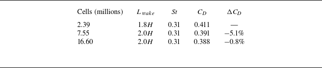
 ΔCD
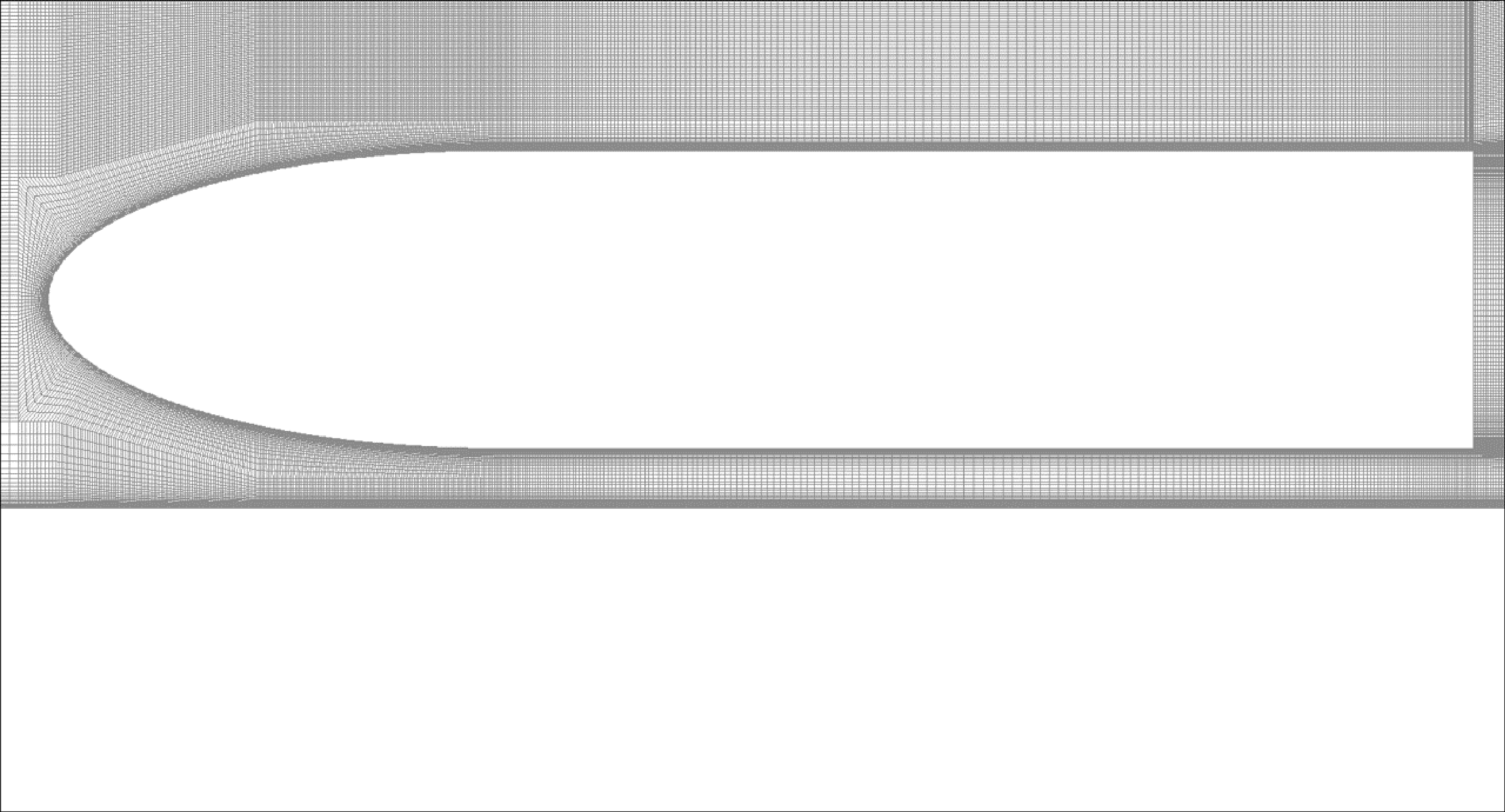

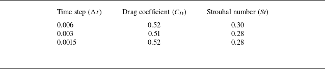
 Δt
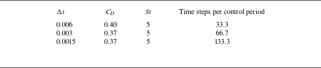
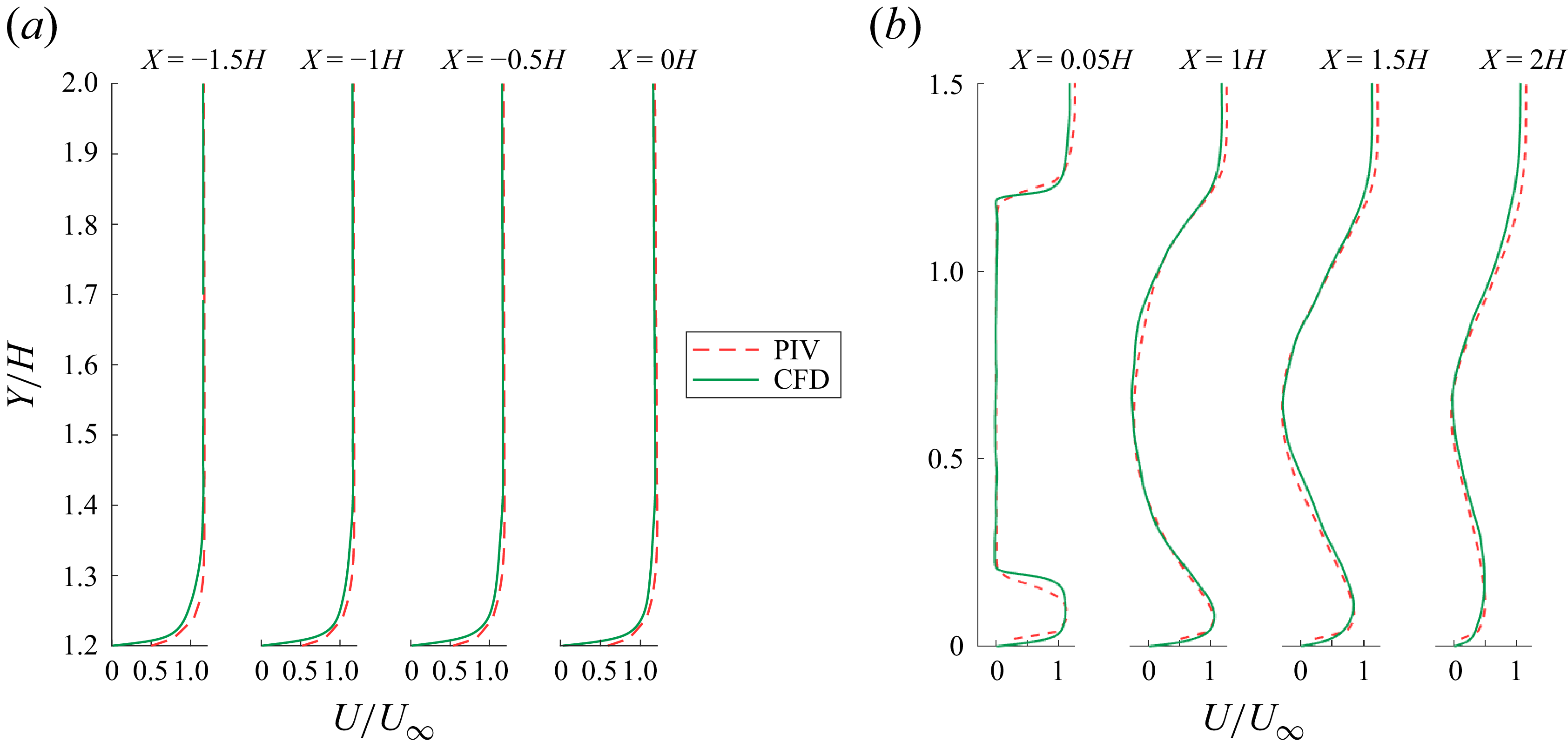
 a
 b


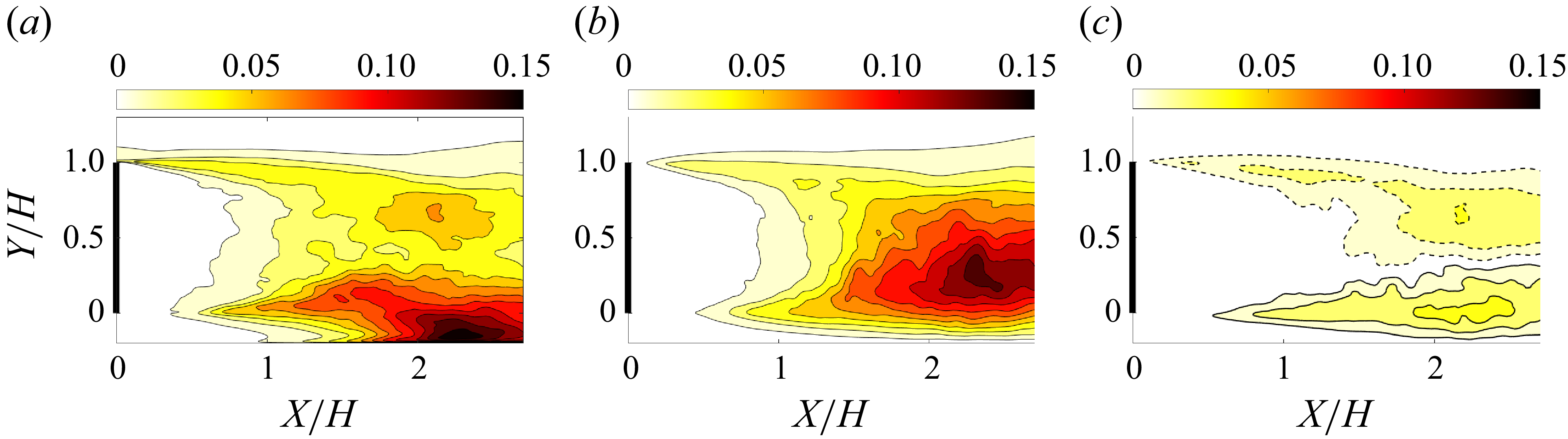
 a
 u′u′¯/U∞2
 b
 v′v′¯/U∞2
 c
 u′v′¯/U∞2
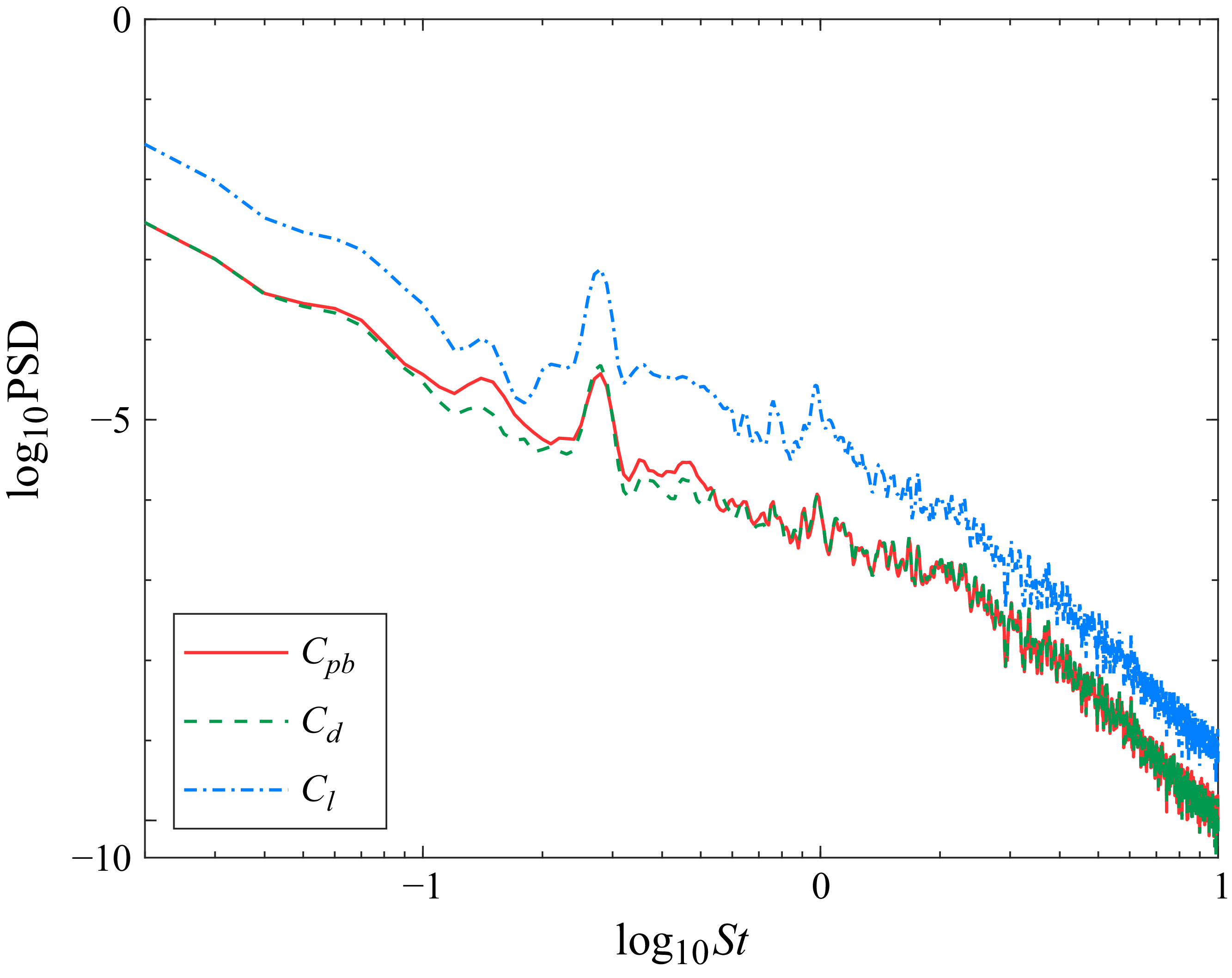


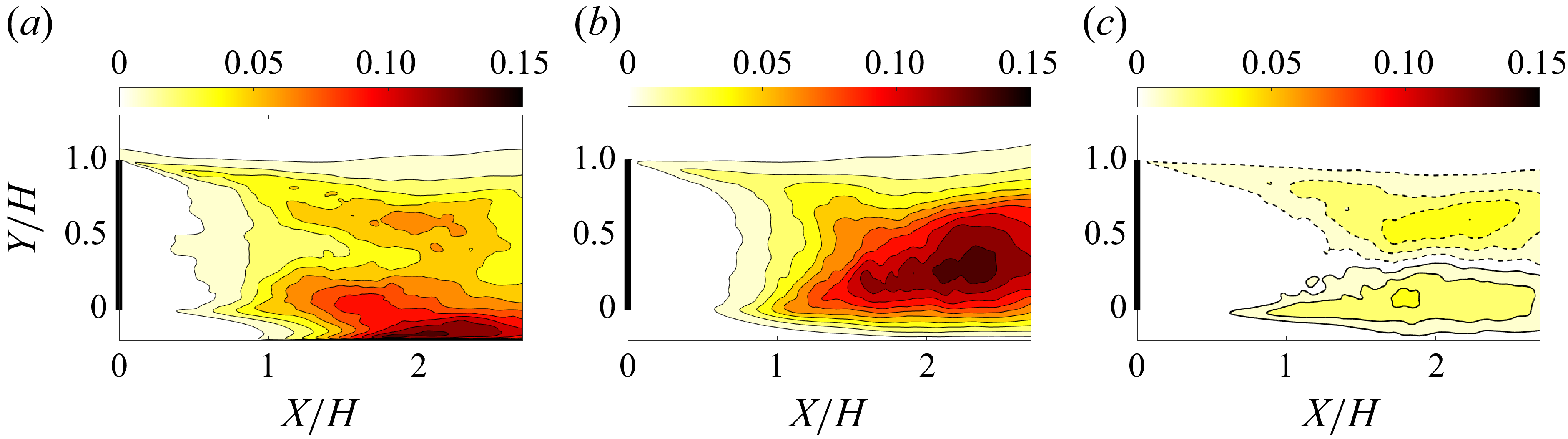
 a
 u′u′¯
 b
 v′v′¯
 c
 u′v′¯

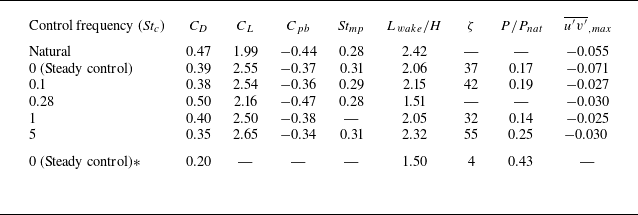
 Stmp
 Lwake
 ζ
 P/Pnat)
 u′v′¯
 ∗
 Cμ=0.06
 Cμ=0.006

 a
 b
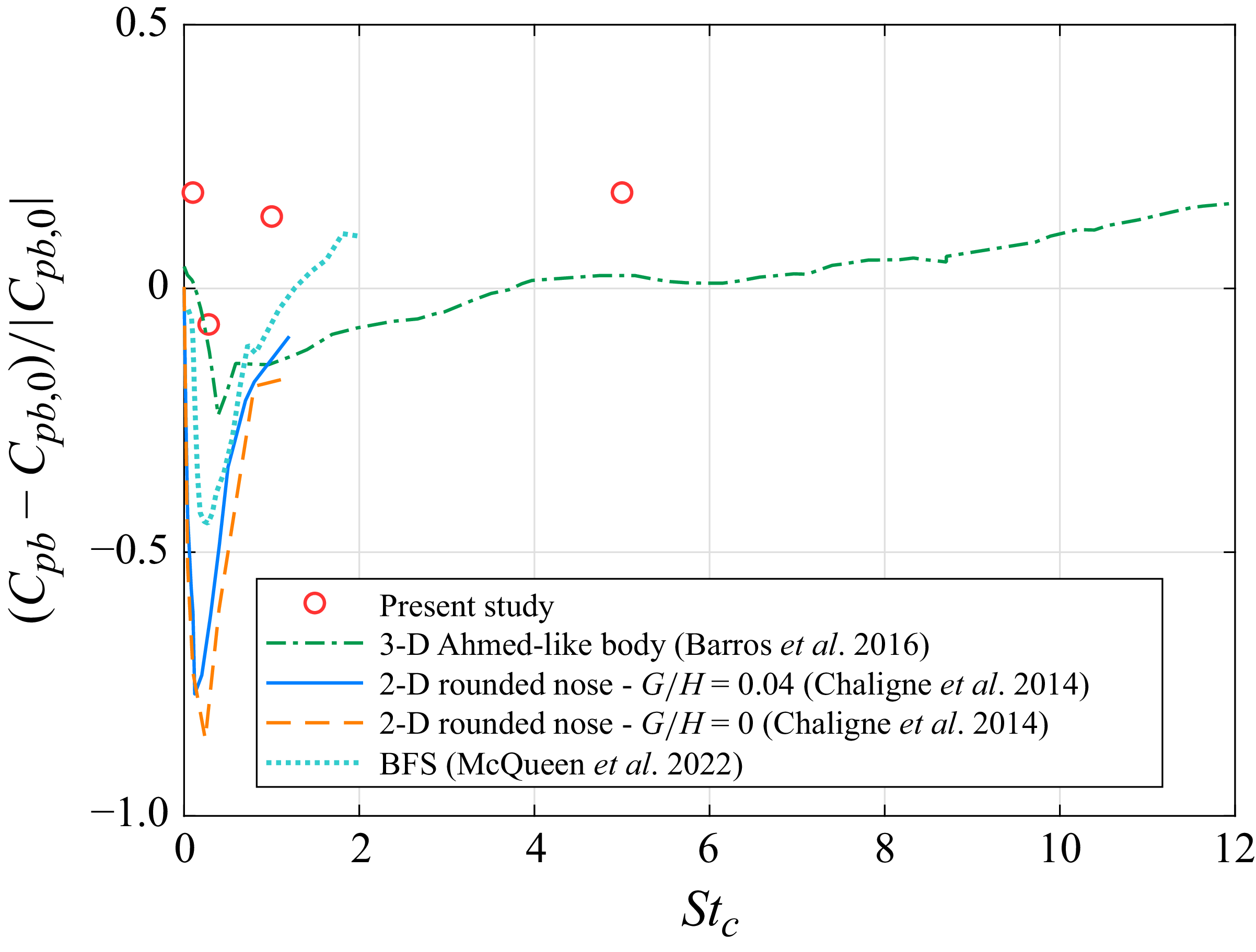
 Cμ
 Cμ

 Stc=0.1
 ⋅
 ⋅
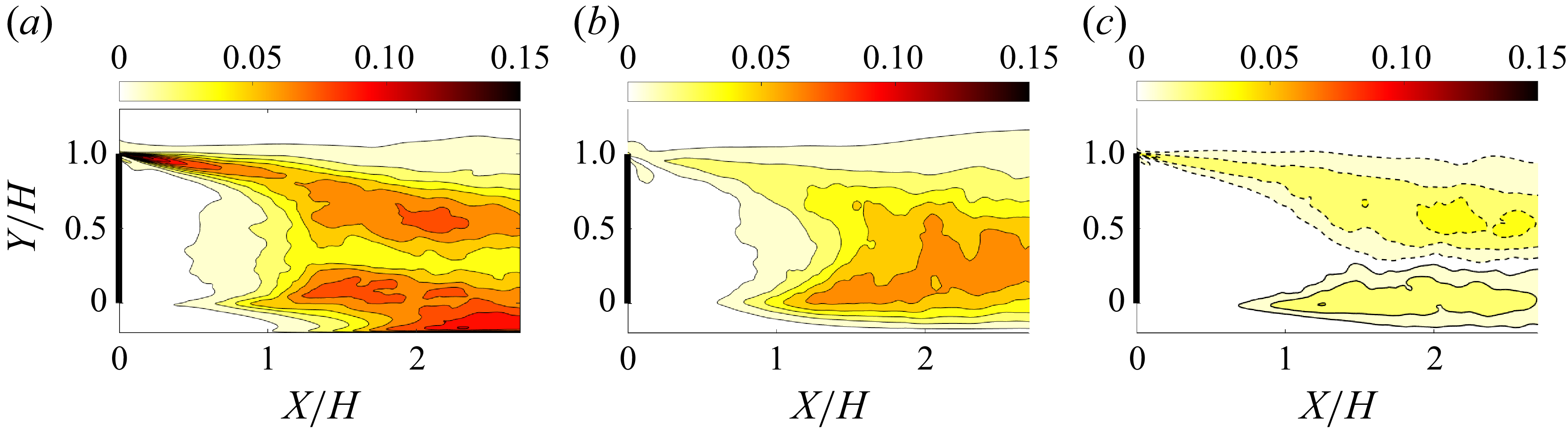
 Stc=0.1
 a
 u′u′¯/U∞2
 b
 v′v′¯/U∞2
 c
 u′v′¯/U∞2

 a
 b
 Stc=0.1

 Stc=0.1

 Stc=0.28
 ⋅
 ⋅

 Stc=0.28
 a
 u′u′¯/U∞2
 b
 v′v′¯/U∞2
 c
 u′v′¯/U∞2

 Stc=0.28

 Stc=1
 ⋅
 ⋅

 Stc=5
 ⋅
 ⋅

 Stc=1
 a
 u′u′¯/U∞2
 b
 v′v′¯/U∞2
 c
 u′v′¯/U∞2
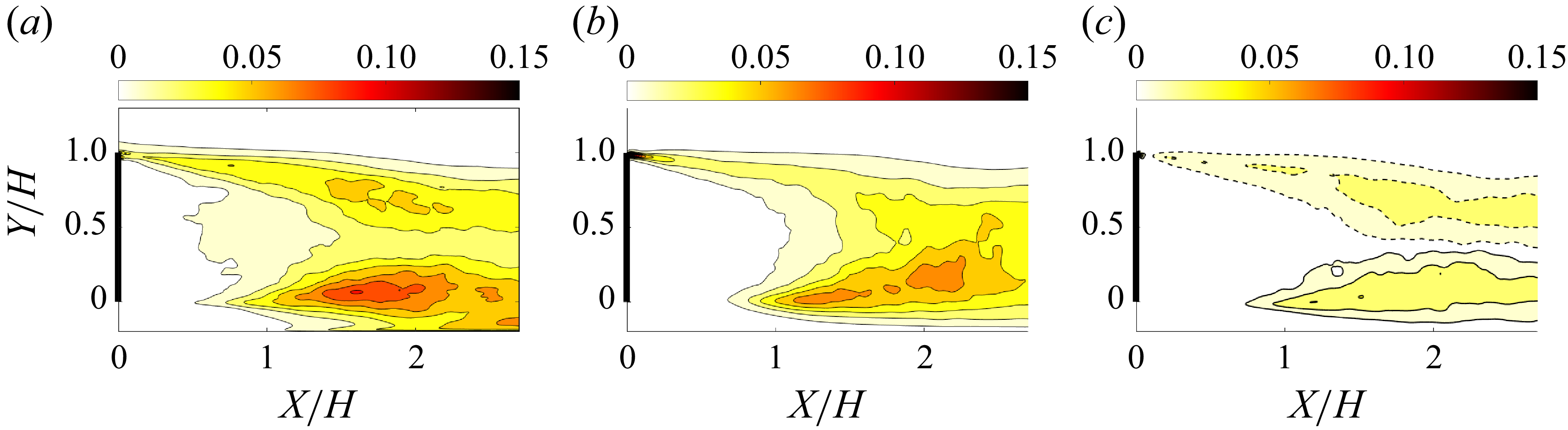
 Stc=5
 a
 u′u′¯/U∞2
 b
 v′v′¯/U∞2
 c
 u′v′¯/U∞2

 a
 b
 Stc=1

 Stc=1

 a
 b
 Stc=5

 Stc=5

 Stc=5

 Stc=5

 a
 b

 −2⟨Q⟩
 −2⟨Q⟩
 St=5

 δ(−2⟨Q⟩)

 Re=2×10⁴
 Cμ=0.06
 CD=0.47
 0.20

 Open access

