





1. Introduction
Delaying transition to turbulence in boundary layers is a key strategy for reducing heat fluxes to the wall in the context of supersonic/hypersonic vehicles, which in turn can reduce the weight and cost of thermal protection systems and increase payload capacity. In high-altitude flight, a highly probable transition path is the natural one, where external disturbances grow in amplitude due to linear mechanisms before reaching a threshold for which the linearity hypothesis is no longer valid; then, three-dimensional (3-D) nonlinear mechanisms appear before vortex breakdown and a subsequent fully turbulent flow (Morkovin Reference Morkovin1969).
1.1. Delaying first and second mode breakdowns
In supersonic/hypersonic boundary layers, the linear growth of instabilities can be due to two distinct convectively unstable modes: the first and second modes (Mack Reference Mack1984). At high Mach number (roughly above Mach 3), the inviscid instability mechanism of the first mode comes from the presence of a generalized inflection point in the boundary layer (Lees & Lin Reference Lees and Lin1946; Mack Reference Mack1984) and the amplification rate of the first mode is maximal for 3-D oblique perturbations (making an angle of
 $60^\circ$
degrees with respect to the spanwise direction at Mach 4.5 for the most unstable first mode obtained from a local stability analysis). As soon as the first mode dominates, the first mode oblique breakdown is considered to be a likely path from laminar to turbulent flow (Mayer et al. Reference Mayer, Von, Dominic and Fasel2011; Franko & Lele Reference Franko and Lele2013; Laible & Fasel Reference Laible and Fasel2016; Unnikrishnan & Gaitonde Reference Unnikrishnan and Gaitonde2019): the nonlinear interaction of two oblique waves (with opposite wave angles) generates streamwise vortices and then streamwise streaks which undergo secondary bifurcation, leading to turbulent flow. Concerning the second mode, called the second Mack mode, it results from the presence of a region where the streamwise base-flow velocity relative to the disturbance phase velocity is supersonic, implying that acoustic noise is trapped in this region (Lees & Lin Reference Lees and Lin1946; Mack Reference Mack1984; Fedorov Reference Fedorov2011). It is characterized by maximum amplification rates for two-dimensional (2-D), i.e. spanwise invariant, waves. Second Mack mode breakdown occurs when the 2-D waves grow sufficiently and saturate, leading to the growth of secondary oblique instabilities and then stationary streaks (Adams & Kleiser Reference Adams and Kleiser1996; Franko & Lele Reference Franko and Lele2013; Sivasubramanian & Fasel Reference Sivasubramanian and Fasel2015; Hader & Fasel Reference Hader and Fasel2019).
Delaying breakdown to turbulence in supersonic/hypersonic flow has been the focus of numerous control studies. One successful approach demonstrated by Sharma et al. (Reference Sharma, Shadloo, Hadjadj and Kloker2019) is the control of full oblique-type breakdown of a supersonic adiabatic boundary layer by employing streaks. Jahanbakhshi & Zaki (Reference Jahanbakhshi and Zaki2021) utilized the sensitivity of instability modes to temperature by wall heating/cooling in order to postpone transition to turbulence under nonlinearly most dangerous free stream disturbance conditions that cause the earliest breakdown. Similarly, Celep et al. (Reference Celep, Hadjadj, Shadloo, Sharma, Yildiz and Kloker2022) employed a combination of streak generation and wall heating/cooling to control the first mode oblique-breakdown in a supersonic boundary layer. Concerning the second Mack mode, Tian et al. (Reference Tian, Liu, Wang, Zhu and Wen2022) managed to drastically decrease its linear growth over a relatively wide frequency range using an acoustic metasurface consisting of two layers of perforated plates, which would potentially delay the second Mack mode breakdown. Furthermore, Jahanbakhshi & Zaki (Reference Jahanbakhshi and Zaki2023) demonstrated that 2-D roughness has a clear impact on the amplification of the second-mode instabilities and used it to disrupt the phase of the near-wall pressure waves, suppress the amplification of the primary instability waves and mitigate the nonlinear interactions that lead to breakdown to turbulence in order to delay it. Zhuang et al. (Reference Zhuang, Wan, Liu, Sun and Lu2024) investigated the use of steady local blowing/suction to delay transition of a flat plate boundary layer at a Mach number of 5.86 and observed that the transition Reynolds number increased by
 $4.6\,\%$
in their breakdown scenario. Nibourel et al. (Reference Nibourel, Leclercq, Demourant, Garnier and Sipp2023, Reference Nibourel, Leclercq, Demourant, Garnier and Sipp2024) were the first to perform reactive control of a supersonic boundary layer by introducing sensors upon which the control action depends. However, transition delay could not be assessed because these studies are two dimensional.
1.2. Reactive control for boundary layer flows
Delaying transition to turbulence with reactive control is inherently more effective than predetermined or passive controls (Gad-el-Hak Reference Gad-el-Hak2001). However, this has only been applied to incompressible boundary layers so far (and many others: Bagheri et al. (Reference Bagheri, Brandt and Henningson2009); Dadfar et al. (Reference Dadfar, Semeraro, Hanifi and Henningson2013); Semeraro et al. (Reference Semeraro, Pralits, Rowley and Henningson2013b ); Sasaki et al. (Reference Sasaki, Morra, Fabbiane, Cavalieri, Hanifi and Henningson2018); Tol et al. (Reference Tol, Kotsonis and Visser2019); Freire et al. (Reference Freire, Cavalieri, Silvestre, Hanifi and Henningson2020); Audiffred et al. (Reference Audiffred, Cavalieri, Brito and Martini2023)). For these boundary layer flows, which fall into the category of noise-amplifier flows (flows sensitive to external disturbances (Huerre & Monkewitz Reference Huerre and Monkewitz1990)), the control strategy is to target the early stages of transition before nonlinear 3-D effects become too significant. This strategy is motivated both by the physics of modal transition mechanisms, and the linear nature of most classical control tools for system identification and controller synthesis. Destructive interference is realized by generating small-perturbations with actuators that take advantage of the linear instability mechanisms to grow and eventually cancel the noise-induced perturbations. Hence, thanks to fully linear control approach, Semeraro et al. (Reference Semeraro, Bagheri, Brandt and Henningson2013a ), Morra et al. (Reference Morra, Sasaki, Hanifi, Cavalieri and Henningson2020) and Sasaki et al. (Reference Sasaki, Morra, Cavalieri, Hanifi and Henningson2020) succeeded in delaying transition to turbulence in a fully nonlinear 3-D incompressible boundary layer.
However, in addition to reducing the amplitude of perturbations or delaying transition to turbulence at the nominal operating point, it is essential to develop robust control strategies that can maintain performance in off-design conditions. Indeed, in practical scenarios such as experimental or flight conditions, the environment is often subject to uncertainties (e.g. free stream variations, acoustic perturbations, surface roughness, nonlinearities, noisy sensors, etc.). For a feedforward configuration (estimation sensors placed upstream of actuators), stability robustness is not an issue and only performance robustness needs to be considered. In particular, performance can generally be preserved despite noisy estimation sensors (Sasaki et al. Reference Sasaki, Morra, Fabbiane, Cavalieri, Hanifi and Henningson2018; Nibourel et al. Reference Nibourel, Leclercq, Demourant, Garnier and Sipp2023), nonlinearities (Morra et al. Reference Morra, Sasaki, Hanifi, Cavalieri and Henningson2020; Sasaki et al. Reference Sasaki, Morra, Cavalieri, Hanifi and Henningson2020), free stream density variations (Nibourel et al. Reference Nibourel, Leclercq, Demourant, Garnier and Sipp2023) or even substantial modifications in transfer function gain simulating changes in instability growth rates (Nibourel et al. Reference Nibourel, Leclercq, Demourant, Garnier and Sipp2024). However, accommodating free stream velocity variations – which alter the convection speed between sensors and actuators – has emerged as a major challenge. Indeed, a simple linear-time-invariant (LTI) feedforward controller may fail when phase variations around the nominal case occur, as convective-delay shifts induced by changes in the upstream free stream velocity can significantly alter the sensor–actuator phase relationship (Fabbiane et al. Reference Fabbiane, Semeraro, Bagheri and Henningson2014, Reference Fabbiane, Simon, Fischer, Grundmann, Bagheri and Henningson2015; Nibourel et al. Reference Nibourel, Leclercq, Demourant, Garnier and Sipp2023, Reference Nibourel, Leclercq, Demourant, Garnier and Sipp2024). Such out-of-phase actuation may lead to constructive rather than destructive interference, thereby promoting instead of delaying transition. To mitigate this issue in the presence of free stream velocity variations, Nibourel et al. (Reference Nibourel, Leclercq, Demourant, Garnier and Sipp2024) attempted to design their feedforward controller using either multimodel synthesis (a single LTI controller optimized over multiple operating points) or gain scheduling (interpolation of several LTI controllers designed for different operating points). However, both strategies resulted in significant performance loss under off-design conditions. Fabbiane et al. (Reference Fabbiane, Simon, Fischer, Grundmann, Bagheri and Henningson2015) preserved the performance of their feedforward controller by employing an adaptive filtered-X least-mean-squares algorithm (Erdmann et al. Reference Erdmann, Pätzold, Engert, Peltzer and Nitsche2011). Yet, this approach only provides robustness over long time scales (i.e. low-frequency variations), as the controller coefficients adapt quasistatically to changes in free stream velocity.
This shortcoming of the feedforward set-up highlights the strong relevance of the feedback set-up (estimation sensors placed downstream the actuators) for performance robustness in convectively unstable flows (Nibourel et al. Reference Nibourel, Leclercq, Demourant, Garnier and Sipp2023). Indeed, the feedback configuration provides performance robustness against phase variations (Nibourel et al. Reference Nibourel, Leclercq, Demourant, Garnier and Sipp2024). But contrary to the feedforward configuration, which is unconditionally stable, stability margins need to be enforced to prevent the instability of the feedback loop in case of errors/uncertainties. As this cannot be realized by the linear–quadratic–Gaussian (LQG) synthesis (Doyle Reference Doyle1978), Belson et al. (Reference Belson, Semeraro, Rowley and Henningson2013) and Vemuri et al. (Reference Vemuri, Bosworth, Morrison and Kerrigan2018) used loop-shaping to design feedback controllers mitigating the linear growth of Tollmien–Schlichting waves. However, the loop-shaping approach cannot easily handle several mathematical criteria at a time, which is a limiting factor for complex specifications that can be encountered in flow control applications. Nibourel et al. (Reference Nibourel, Leclercq, Demourant, Garnier and Sipp2023, Reference Nibourel, Leclercq, Demourant, Garnier and Sipp2024) employed the multicriteria structured mixed
 $H_2/H_\infty$
synthesis (Apkarian et al. Reference Apkarian, Gahinet and Buhr2014). This synthesis method allows us to fix beforehand the controller structure and to minimize appropriate norms of various transfer functions to handle simultaneously in an optimal way the problem of nominal performance, stability robustness and performance robustness.
1.3. Centralized/decentralized configurations
Nevertheless, as structured syntheses are solved via non-smooth/non-convex optimization techniques (Apkarian et al. Reference Apkarian, Noll and Rondepierre2010, Reference Apkarian, Dao and Noll2015), their resolution may be computationally intensive (compared with an optimal synthesis): non-smooth algorithms are more complex and have higher computational costs than smooth algorithms (which presume certain differentiability and strong regularity assumptions) and several initializations of the controller parameters are needed to deal with the non-convex nature of the problem. Hence, to enable the resolution via this synthesis method, it is necessary to have low-dimensional problems, which may not be straightforward for 3-D cases where multiple sensors and actuators are required.
To reduce the complexity of synthesis in cases with a large number of parameters, a decentralized approach can be used to limit interconnections between inputs and outputs, where only subsets of inputs are connected to subsets of outputs, as opposed to a centralized configuration where all inputs are connected to all outputs (Bamieh et al. Reference Bamieh, Paganini and Dahleh2002; Bagheri & Henningson Reference Bagheri and Henningson2011). In the case of 2-D plane Poiseuille flow, the streamwise direction is homogeneous, therefore the state-space model can be put in diagonal form in the streamwise wavenumber space (Joshi et al. Reference Joshi, Speyer and Kim1997). To respect the Nyquist–Shannon sampling theorem, it is required to have a spacing of each sensor/actuator smaller than half the minimum wavelength found in the wavenumber spectrum in order to resolve and cancel any growing disturbances (Li & Gaster Reference Li and Gaster2006). The whole state-space system is consequently equivalent to
 $N$
state-space subsystems, one for each wavenumber. This enabled Cortelezzi et al. (Reference Cortelezzi, Speyer, Lee and Kim1998) and Högberg et al. (Reference Högberg, Bewley and Henningson2003) to tackle the 3-D plane Poiseuille flow case by designing
 $N$
controllers through LQG synthesis, one for each streamwise/spanwise wavenumber pairs, instead of one high-order controller that would have been to hard to design.
Note that using the Fourier space is limited to flows with a homogeneous direction. Therefore, to develop a more generic approach that can be applied to a wider range of flows, some studies on boundary layer control remained in the physical space and used a decentralized approach where only a subset of sensors are connected to the actuators (Semeraro et al. Reference Semeraro, Bagheri, Brandt and Henningson2011, Reference Semeraro, Bagheri, Brandt and Henningson2013a ; Dadfar et al. Reference Dadfar, Fabbiane, Bagheri and Henningson2014). More recently, Sasaki et al. (Reference Sasaki, Morra, Fabbiane, Cavalieri, Hanifi and Henningson2018), Morra et al. (Reference Morra, Sasaki, Hanifi, Cavalieri and Henningson2020) and Sasaki et al. (Reference Sasaki, Morra, Cavalieri, Hanifi and Henningson2020) designed controllers directly in the spanwise wavenumber space for the incompressible boundary layer case in order to delay transition to turbulence. Yet, these studies synthesized controllers in the wavenumber space with an inverse method or LQG synthesis, both with a feedforward architecture, which raises the problem of performance robustness of their controllers in case of free stream velocity variations.
1.4. Objective and outline of the paper
The novelty of the present paper lies in employing a reactive control strategy to derive a robust control law. This approach combines a feedback architecture with multicriteria structured synthesis, with the objective of delaying transition to turbulence in a supersonic boundary layer by simultaneously mitigating the growth of both first and second modes, while also ensuring robustness with respect to free stream velocity variations.
We consider transition delay in a supersonic boundary layer at
 $M_{\infty }=4.5$
using reactive control through direct numerical simulations (DNS). This study is an extension of Nibourel et al. (Reference Nibourel, Leclercq, Demourant, Garnier and Sipp2023, Reference Nibourel, Leclercq, Demourant, Garnier and Sipp2024) where only spanwise invariant and linear perturbations were considered. In the 3-D set-up, oblique waves are also present and the feedback control law needs to target both the early growth of the first and second instability modes. Similar to previous work, the approach is fully linear and data-driven. Models are obtained using system identification and controllers are realized using structured mixed
 $H_2/H_{\infty }$
synthesis.
The paper is organized as follows. Section 2 provides a description of the flow configuration and methods. Section 3 shows how to transform the centralized problem in the physical space to a decentralized problem in the spanwise wavenumber domain for the structured mixed
 $H_2/H_\infty$
, making identification and synthesis feasible. In § 4, the fluid specifications are reinterpreted from a control perspective, enabling the introduction of key robust control principles. Section 5 is devoted to the control settings, as well as the characterization of the noise-amplifier behaviour of the 3-D flow in the linear regime. Then the identification of the reduced-order models (ROMs) and the several constrained minimization problems (CMP) solved are presented in § 6. Finally, the control efficiency in both the linear and transitional regimes is assessed in § 7. Conclusions are drawn in § 8.
2. Flow configuration and methods
2.1. Computational flow set-up
We consider the Navier–Stokes equations for a 3-D compressible ideal gas flowing over a flat plate,
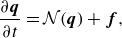 \begin{align} \frac {\partial \boldsymbol{q}}{\partial t}=\mathcal{N}(\boldsymbol{q})+\boldsymbol{f}, \end{align}
where
 $\boldsymbol{q}=[\rho, \rho \boldsymbol{v}, \rho E]^{T}$
is the state vector of conservative variables comprising the fluid density
 $\rho$
, the velocity vector
 $\boldsymbol{v}$
and the total energy
 $E=( {p}/({\rho (\gamma -1)}))+({1}/{2})\boldsymbol{v}\boldsymbol{\cdot }\boldsymbol{v}$
(
 $p$
is the static pressure and
 $\gamma =1.4$
is the ratio of specific heats). The dynamic viscosity
 $\mu$
is computed via Sutherland’s law from the local static temperature
 $T={p}/{\rho r}$
with
 $r=287\ \mathrm{J\,K^{-1}\,kg^{-1}}$
the perfect gas constant. The forcing term
 $\boldsymbol{f}$
represents the noise sources or the impact of actuators on the flow.
The free stream flow conditions are those used in Nibourel et al. (Reference Nibourel, Leclercq, Demourant, Garnier and Sipp2023, Reference Nibourel, Leclercq, Demourant, Garnier and Sipp2024) in their 2-D configuration, i.e.
 $T_{\infty }=65.149 \ \mathrm{K}$
,
 $ V_{\infty }=728.191\ \mathrm{m\,s^{-1}}$
and
 $p_{\infty }=728.312\ \mathrm{Pa}$
. Thus, the free stream Mach number of the simulation is
 $M_{\infty }={V_{\infty }}/{\sqrt {\gamma rT{\infty }}}=4.5$
.
The 3-D computational domain used for the linearized DNS (where perturbations remain in the linear regime, see §§ 5 and 7.1) is represented in figure 1. The streamwise, wall-normal and spanwise directions are denoted
 $x_1$
,
 $x_2$
and
 $x_3$
, respectively. The 3-D computational domain consists of the 2-D numerical domain used in Nibourel et al. (Reference Nibourel, Leclercq, Demourant, Garnier and Sipp2023, Reference Nibourel, Leclercq, Demourant, Garnier and Sipp2024) and extruded over the span
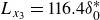 $L_{x_3}=116.4\delta _0^*$
in the transverse direction, with
 $\delta _{0}^{*}=3.2656 \times 10^{-4}\ \mathrm{m}$
(defined as
 $\delta _{0}^{*}=\int ^{\infty }_{0} (1-({\rho v_{x_1}}/{\rho _{\infty }V_{\infty }})){\rm d}x_2$
) the compressible displacement thickness at the inlet of the domain. The lower boundary is an adiabatic flat plate of length
 $L_{x_1}=2002.1\delta _{0}^{*}$
. A sponge zone is present downstream of the domain to reduce reflections; this sponge zone is obtained by stretching of the mesh in the longitudinal direction (30 cells in the streamwise direction over
 $L_{\textit{sponge}}=91.9\delta _{0}^{*}$
). Periodic, far-field and supersonic exit conditions are, respectively, applied at the sides, top (
 $x_2=275.\delta _0^*$
) and outlet of the domain. Concerning the supersonic inlet condition, the full state vector is prescribed and corresponds to a zero-pressure gradient laminar boundary layer profile taken at a distance of
 $19\delta _{0}^{*}$
from the leading edge. Overall, the useful numerical domain (i.e. not counting the length of the sponge area) expands from
 $4\times 10^{4}\lt Re_{x_1}=( {\rho _{\infty }V_{\infty }x_1}/{\mu _{\infty }})\lt 4.1\times 10^{6}$
.
Diagram of the 3-D computational domain used for linearized DNS. The red shaded region represents the sponge zone.
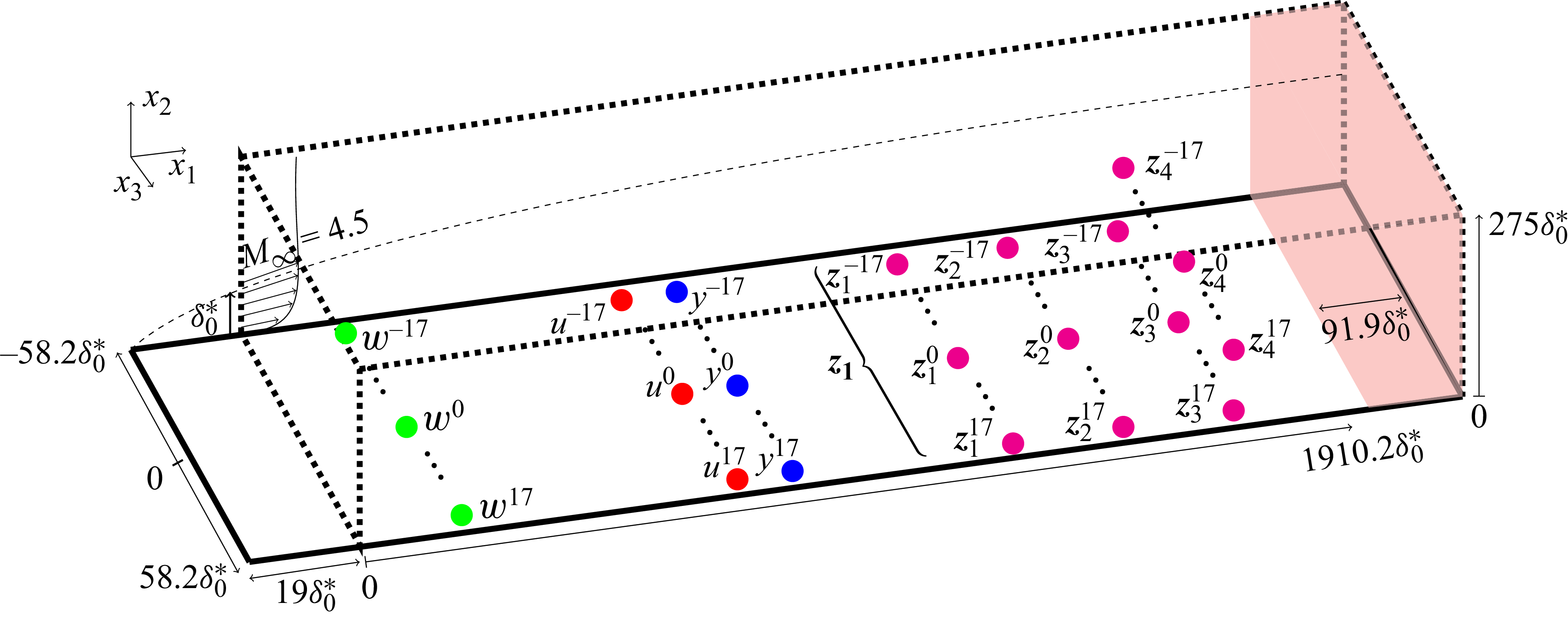
Figure 1. Long description
A diagram of a 3-D computational domain used for linearized DNS. The red shaded region represents the sponge zone. The diagram includes multiple labeled points and regions, such as w, u, v, and z, with different superscripts and subscripts indicating their positions and roles within the domain. The axes are labeled with x1, x2, and x3, and specific values are marked along these axes. The diagram illustrates the spatial relationships and positions of these points within the computational domain, showing how they interact and contribute to the overall structure.
2.2. The DNS solver
The 3-D DNS of the fully compressible Navier–Stokes equations are performed with the in-house research solver FastS (Peron et al. Reference Peron, Renaud, Mary, Benoit and Terracol2017). An upwind AUSMP
 $^{+}$
scheme (Liou & Edwards Reference Liou and Edwards1999; Liou Reference Liou2006) associated with a third-order MUSCL (monotonic upstream-centered scheme for conservation laws) extrapolation method (Leer Reference Leer1979) is used for the spatial discretization of the convective fluxes. The viscous fluxes are obtained by a second-order centred scheme. For the linearized DNS (see §§ 5 and 7.1), a resolution of
 $3200\times 220\times 176$
cells for the useful domain (i.e. not including the downstream sponge zone) is chosen with a uniform mesh in the
 $x_1$
and
 $x_3$
directions and a geometric law in the
 $x_2$
direction. For the DNS of transition to turbulence (see § 7.2), the length and the number of grid points are doubled in the longitudinal direction in order to reach transition by the downstream end of the computational domain while remaining weakly nonlinear at the streamwise position of the estimation sensors.
The laminar base-flow
 $ \boldsymbol{\bar {q}}$
, defined as
 \begin{align} \mathcal{N}(\boldsymbol{\bar {q}})=0, \end{align}
is obtained by time stepping the unforced (i.e.
 $\boldsymbol{f}=0$
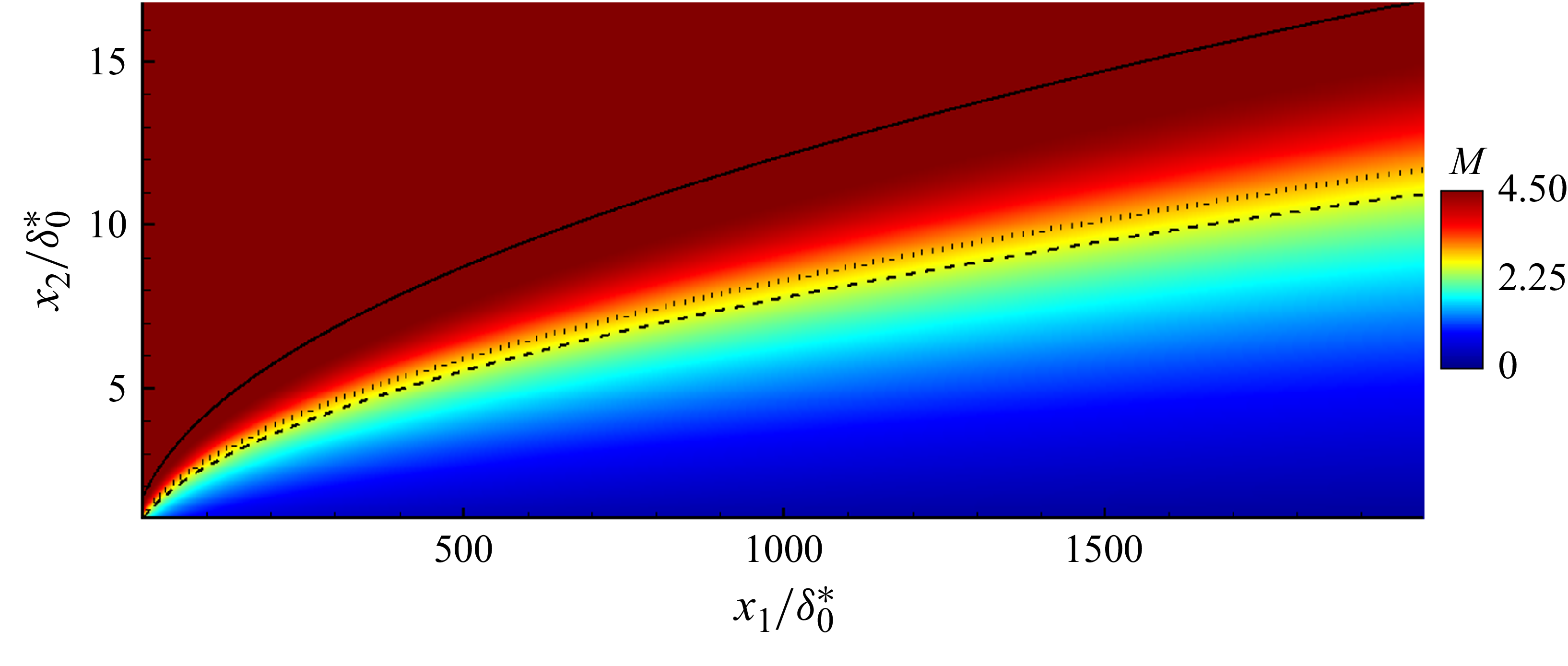
) unsteady (2.1) with an implicit time stepping method based on a local time step, up to convergence of the residuals. The Mach number field of the laminar base flow is shown in figure 2, along with the boundary layer thickness
 $\delta$
(solid line), the compressible displacement thickness
 $\delta ^{*}$
(dashed line) and the generalized inflection point
 $x_{2,\textit{GIP}}$
(dotted line), defined by
 \begin{align} \left .\partial _{x_2} \left (\bar {\rho } \partial _{x_2} \bar {v}_{x_1}\right )\right |_{x_{2,\textit{GIP}}}=0, \end{align}
which plays an important role in the development of instabilities (Mack Reference Mack1984; Bugeat et al. Reference Bugeat, Chassaing, Robinet and Sagaut2019; Nibourel et al. Reference Nibourel, Leclercq, Demourant, Garnier and Sipp2023). The boundary-layer thickness
 $\delta$
is computed using a diagnostic function combining wall distance and vorticity. The details of the method, as well as the coefficients of the diagnostic function, are given in Bégou et al. (Reference Bégou, Maugars, Andrieu and Deniau2025). Other boundary-layer quantities (
 $\delta ^*$
,
 $x_{2,\textit{GIP}}$
) are subsequently evaluated within this thickness, either by integration from the wall to
 $\delta$
or by identification of relevant flow features within this region.
Mach number field of the
 $x_3$
-homogeneous laminar base flow. Solid, dotted and dashed lines represent the boundary layer thickness
 $\delta$
, the generalized inflection point
 $x_{2,\textit{GIP}}$
and the compressible displacement thickness
 $\delta ^{*}$
, respectively.
The 3-D unsteady simulations use an explicit third-order three-steps low-storage Runge–Kutta scheme (Williamson Reference Williamson1980) with a time step ensuring a Courant–Friedrichs–Lewy (CFL) number lower than
 $0.7$
(respectively,
 $0.4$
) in the whole domain for the linearized DNS (respectively, the nonlinear DNS that leads to transition to turbulence). The time step of the fully nonlinear DNS that lead to transition is lower compared with the one of the linearized DNS for stability reasons. For the linearized 3-D unsteady simulations, since the code is fully nonlinear, the amplitude of the forcing
 $\boldsymbol{{f}}$
is chosen sufficiently small to ensure that the induced perturbation
 $\boldsymbol{{q}'}=\boldsymbol{{q}}-\boldsymbol{\bar {q}}$
remains in the linear regime until the end of the computational domain. Convergence tests for grid and time step independence are reported in Appendix A. The evolution along the streamwise direction of the amplitude (which depends on frequency and spanwise wavenumber) of pressure instability at
 $x_2=0$
and velocity instability at
 $x_2=x_{2,\textit{GIP}}$
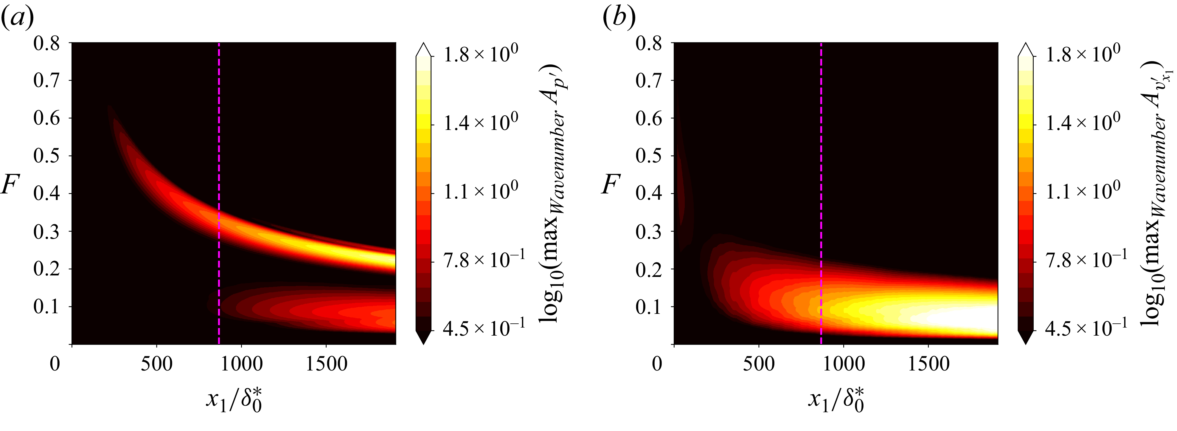
induced by exogenous disturbances is shown in figure 3. The choice of system inputs and outputs leading to this representation is detailed in §§ 3 and 5; the figure is introduced here only to illustrate the intrinsic difficulty of instability control at Mach 4.5 due to the combined effects of wide bandwidths, multiple spanwise scales and the wall-normal dependence of the dominant mode. The wall-pressure instabilities exhibit two distinct lobes: the upper lobe corresponds to the high-frequency, low–spanwise-wavenumber content of the second Mack mode, whereas the lower lobe corresponds to the low-frequency, higher-spanwise-wavenumber content of the first mode. Wall-pressure sensors are primarily sensitive to the second Mack mode, while velocity fluctuations measured at the generalized inflection point are sensitive only to the first mode. The larger the streamwise extent of the control region and the lower the Reynolds number at its onset, the broader the frequency bandwidth that must be controlled over the domain. Note that the wider the bandwidth to be controlled, the more difficult it becomes to achieve high attenuation across the entire spectrum (Nibourel et al. Reference Nibourel, Leclercq, Demourant, Garnier and Sipp2023). This reflects a trade-off similar to the waterbed effect (Skogestad & Postlethwaite Reference Skogestad and Postlethwaite2005): robustness, stability and feasibility constraints prevent uniformly reducing disturbance amplitude over all frequencies, such that attenuating some frequencies inevitably leads to amplification at others.
Evolution along the streamwise direction of the amplitude (which depends on frequency and spanwise wavenumber) of (a) pressure instability at
 $x_2=0$
and (b) velocity instability at
 $x_2=x_{2,\textit{GIP}}$
induced by exogenous disturbances. The vertical magenta lines represent the streamwise position of the actuators used in this paper.
3. From a centralized to a decentralized control approach
In § 3.1 we formally introduce the inputs and outputs in order to explain in § 3.2 how we transform a large centralized control problem into a fully decentralized one, by exploiting symmetries of our control set-up. The physical justification for the specific choices of sensors we make is left for § 5 where we investigate the uncontrolled and open-loop dynamics of the flow. In § 3.3, we explain how we deal with the fact that noise sources cannot be directly measured. In § 3.4, we explain why convection delays from actuator to performance sensors may be safely ignored in our control set-up, to speed up system identification and controller synthesis. Finally, in § 3.5 we provide formal constraints for choosing the number of actuators and sensors in § 5.
3.1. Inputs and outputs
The control set-up consists of spanwise-periodic rows of actuators
 $u^i$
, estimation sensors
 $y^i$
and performance sensors
 $z_{\kern-1pt j}^i$
. In each case, the superscript
 $i$
indexes the spanwise location, with elements of identical type uniformly spaced by
 $\varDelta _{x_3} = 3.32 \delta _0^*$
and operating independently. While a single row is used for the actuators and estimation sensors, four streamwise rows of performance sensors are considered, indexed by
 $j = 1, \ldots, 4$
(see figure 1). In addition, to create instabilities in the flow, a spanwise-periodic row of exogenous disturbances
 $w^i$
is used. In the spanwise-direction
 $x_3$
, the computational domain comprises
 $n = 2m+1$
actuators and sensors (
 $m=17$
so
 $n=35$
); hence the flow field is periodic in the spanwise direction with period
 $L_{x_3}=n\varDelta _{x_3}$
. It should be noted that the number of spanwise exogenous disturbances
 $w^i$
need not match the number of sensors and actuators for the development of the method, as the controller synthesis is performed solely based on the available signals
 $y^i$
,
 $u^i$
and
 $z^i$
(see § 3.3). The number of sensors (
 $y^i$
,
 $z^i$
) within each row coincides with the number of actuators
 $u^i$
and this choice is justified § 3.5. The physical rationale for the input and output configuration (streamwise locations, types, spanwise spacing, number of rows, etc.) is detailed in § 5, the present section focusing mainly on establishing the control framework. Input and output variables may be gathered in column vectors of
 $\mathbb{R}^n$
,
 \begin{align} \boldsymbol{w}&=[w^{-m},\ldots, w^0,\ldots w^m]^T,\quad &\boldsymbol{u}=[u^{-m},\ldots, u^0,\ldots u^m]^T, \\[-12pt] \nonumber \end{align}
 \begin{align} \boldsymbol{y}&=[y^{-m},\ldots, y^0,\ldots y^m]^T,\quad &\boldsymbol{z}_{\!j}=[z_{\kern-1pt j}^{-m},\ldots, z_{\kern-1pt j}^0,\ldots z_{\kern-1pt j}^m]^T. \\[10pt] \nonumber \end{align}
The forcing field
 $\boldsymbol{f}$
in (2.1) is taken as the sum of a noise term (acoustic perturbations, surface roughness, free stream turbulence, entropy spot, etc.)
 $\boldsymbol{f}_{\boldsymbol{w}}$
and an actuator term
 $\boldsymbol{f}_{\boldsymbol{u}}$
,
 \begin{align} \boldsymbol{f}_{\boldsymbol{w}}(x_1,x_2,x_3,t)&=\epsilon \boldsymbol{g}(x_1-x_{1,\boldsymbol{w}}, \, x_2-\delta _0^*; \, \sigma _{x_1}, \, \sigma _{x_1}/10)\sum _{i=-m}^m B_{w^i}(x_3)w^i(t), \\[-28pt] \nonumber \end{align}
 \begin{align} \boldsymbol{f}_{\boldsymbol{u}}(x_1,x_2,x_3,t)&=\epsilon \boldsymbol{g}(x_1-x_{1,\boldsymbol{u}}, \, x_2-x_{2,\textit{GIP}}(x_{1,\boldsymbol{u}});\, \sigma _{x_1}, \, \sigma _{x_1}/3)\sum _{i=-m}^m B_{u^i}(x_3)u^i(t), \\[0pt] \nonumber \end{align}
where
 \begin{align} \boldsymbol{g}(x_1,x_2;\sigma _{x_1},\sigma _{x_2})&=[0,x_2\sigma _{x_1}/\sigma _{x_2},-x_1\sigma _{x_2}/\sigma _{x_1},0,0]^T\mathrm{exp} \!\left (-\dfrac {x_1^2}{2\sigma _{x_1}^2}-\dfrac {x_2^2}{2\sigma _{x_2}^2}\right ), \\[-28pt] \nonumber \end{align}
 \begin{align} B_{w^i}(x_3)&=\sum _{p=-\infty }^\infty b_w(x_3-i\varDelta _{x_3}+pn\varDelta _{x_3}),\quad b_w(x_3)=\delta _{\textit{Dirac}}(x_3), \\[-28pt] \nonumber \end{align}
 \begin{align} B_{u^i}(x_3)&=\sum _{p=-\infty }^\infty b_u(x_3-i\varDelta _{x_3}+pn\varDelta _{x_3}),\quad b_u(x_3)=\mathrm{exp} \!\left (-\dfrac {x_3^2}{2\sigma _{x_3}^2}\right ), \\[0pt] \nonumber \end{align}
with
 $\sigma _{x_1}=1.06\delta _0^*$
,
 $\sigma _{x_3}=4.98\delta _0^*$
and streamwise positions of the rows of exogenous noises
 $x_{1,\boldsymbol{w}}$
and actuators
 $x_{1,\boldsymbol{u}}$
indicated in table 1. The amplitude
 $\epsilon$
is chosen in §§ 6 and 7.1 such that the dynamics is linear throughout the numerical domain. In § 7.2, the amplitude is increased to induce transition to turbulence within the domain. The form of the momentum forcing
 $\boldsymbol{g}$
is identical to that chosen in previous studies of transition to turbulence in incompressible and supersonic boundary layers (Bagheri et al. Reference Bagheri, Brandt and Henningson2009; Semeraro et al. Reference Semeraro, Bagheri, Brandt and Henningson2011; Belson et al. Reference Belson, Semeraro, Rowley and Henningson2013; Nibourel et al. Reference Nibourel, Leclercq, Demourant, Garnier and Sipp2023, Reference Nibourel, Leclercq, Demourant, Garnier and Sipp2024). The noise term
 $\boldsymbol{f_w}$
is localized close to the inlet, at a streamwise position
 $x_{1,\boldsymbol{w}}=4.1\delta _0^*$
, and centred about
 $x_2=\delta _0^*$
in the wall-normal direction. The independent-white-noise-in-time signals
 $w^i(t)$
modulate the amplitude of the spatial supports
 $B_{w^i}$
(which are based on a Dirac comb in the spanwise direction) of the noise sources; hence no spanwise wavenumber or frequency is initially privileged. On the other hand, actuation
 $\boldsymbol{f_u}$
is centred about the generalized inflection point
 $x_2=x_{2,\textit{GIP}}(x_{1,\boldsymbol{u}})$
at the streamwise position
 $x_{1,\boldsymbol{u}}=867.2\delta _0^*$
. The modelling of the actuation impact in the flow as a localized forcing term centred around the generalized inflection point may remain idealized with respect to a practical experimental implementation, although advanced actuation devices such as plasma actuators could potentially approximate such a forcing distribution (Dadfar et al. Reference Dadfar, Semeraro, Hanifi and Henningson2013; Shahriari et al. Reference Shahriari, Kollert and Hanifi2018; Samimy et al. Reference Samimy, Webb and Esfahani2019). The modelling of a realistic actuator nevertheless lies beyond the scope of the present study. We selected this wall-normal position to ease the control of the instabilities by maximizing the receptivity process (Nibourel et al. Reference Nibourel, Leclercq, Demourant, Garnier and Sipp2023). The streamwise position of the actuators
 $x_{1,\boldsymbol{u}}$
is a compromise between controlling a sufficiently long domain representative of experimental configurations and restricting the complexity of the control problem by limiting the frequency–wavenumber range to control (see figure 3). The spatial supports
 $B_{u^i}$
of the actuators are modelled as a comb of Gaussian functions in the spanwise direction, while the signals
 $u^i(t)$
are not known a priori but are determined by the controller based on the estimation sensor signals
 $y^i(t)$
. For both
 $\boldsymbol{f_w}$
and
 $\boldsymbol{f_u}$
, only the
 $x_1$
and
 $x_2$
components of the momentum forcing terms are excited (via the function
 $\boldsymbol{g}$
), which is optimal for the second mode, but suboptimal for the first (oblique) mode, as non-zero transverse momentum forcing would lead to greater growth according to Bugeat et al. (Reference Bugeat, Chassaing, Robinet and Sagaut2019).
Streamwise position of rows of sources and sensors, in units of
 $\delta _0^*$
.

Table 1. Long description
A table with one row and seven columns. The columns are labeled as x1,w, x1,u, x1,y, x1,z1, x1,z2, and x1,z3 = x1,z4. The values in the row are 4.1, 867.2, 887.6, 1022.6, 1312.2, and 1775.0 respectively.
Next we introduce sensors. The row of
 $n=2m+1$
estimation sensors
 $y^i$
(which serve as inputs to the controller) is located at
 $x_{1,\boldsymbol{y}}=887.6\delta _0^*$
and is composed of fluctuation wall-pressure sensors. Following the conclusions of Nibourel et al. (Reference Nibourel, Leclercq, Demourant, Garnier and Sipp2023, Reference Nibourel, Leclercq, Demourant, Garnier and Sipp2024), these estimation sensors are placed downstream of actuators to enforce performance robustness to free stream velocity variations. Therefore, this is a feedback set-up and not a feedforward one as typically found in the literature on noise-amplifier flows. The four rows of
 $n=2m+1$
performance sensors
 $z^i_j$
only serve to define an objective functional for optimizing the controller. Rows
 $1,2,3$
, respectively, located at
 $(x_{1,\boldsymbol{z}_1},\, x_{1,\boldsymbol{z}_2},\, x_{1,\boldsymbol{z}_3})=(1022.6,1612.2,1775.0)\delta _0^*$
, measure fluctuating wall-pressure
 $p'$
. Row
 $4$
is located at
 $x_{1,\boldsymbol{z}_4}=x_{1,\boldsymbol{z}_3}$
and measures longitudinal perturbation velocities
 $v_{x_1}'$
at the generalized inflection point. On each row, sensors are infinitely localized in
 $x_3$
, and regularly spaced in the transverse direction with
 $\varDelta _{x_3}$
. For
 $-m\leqslant i\leqslant m$
, we have
 \begin{align} y^i(t)&=p'(x_{1,\boldsymbol{y}},\, 0,\, i\varDelta _{x_3},\, t), \\[-28pt] \nonumber \end{align}
 \begin{align} z_{\kern-1pt j}^i(t)&=\begin{cases} p'(x_{1,\boldsymbol{z}_{\!j}},\, 0,\, i\varDelta _{x_3},\, t),\quad &j=1,2,3,\\ v_{x_1}'(x_{1,\boldsymbol{z}_{\!j}},\, x_{2,\textit{GIP}}(x_{1,\boldsymbol{z}_{\!j}}),\, i\varDelta _{x_3},\, t),\quad &j=4. \end{cases} \\[-12pt] \nonumber \end{align}
Again, these specific choices will be justified later in § 5.
The linear time-invariant dynamics of the supersonic boundary layer may be described using multiple-input–multiple-output (MIMO) transfer functions which are all functions of the Laplace variable
 $s$
. In the absence of control, the MIMO transfers
 $\boldsymbol{T}_{\!\boldsymbol{yw}}$
and
 $\boldsymbol{T}_{\!\boldsymbol{z}_{\!j}\boldsymbol{w}}$
represent the impact of the disturbances
 $\boldsymbol{w}$
on the sensors
 $\boldsymbol{y}$
and
 $\boldsymbol{z}_{\!j}$
, respectively; i.e.
 $\boldsymbol{y}=\boldsymbol{T_{yw}}\boldsymbol{w}$
and
 $\boldsymbol{z}_{\!j}=\boldsymbol{T}_{\!\boldsymbol{z}_{\!j}\boldsymbol{w}}\boldsymbol{w}$
. The impact of the actuator on the sensors, in the absence of disturbances, is represented by the MIMO transfers
 $\boldsymbol{T}_{\!\boldsymbol{yu}}$
and
 $\boldsymbol{T}_{\!\boldsymbol{z}_{\!j}\boldsymbol{u}}$
; i.e.
 $\boldsymbol{y}=\boldsymbol{T_{yu}}\boldsymbol{u}$
and
 $\boldsymbol{z}_{\!j}=\boldsymbol{T}_{\!\boldsymbol{z}_{\!j}\boldsymbol{u}}\boldsymbol{u}$
. The MIMO transfer function of the controller is denoted
 $\boldsymbol{K}$
and it transforms the measurement signal
 $\boldsymbol{y}$
into the control signal
 $\boldsymbol{u}$
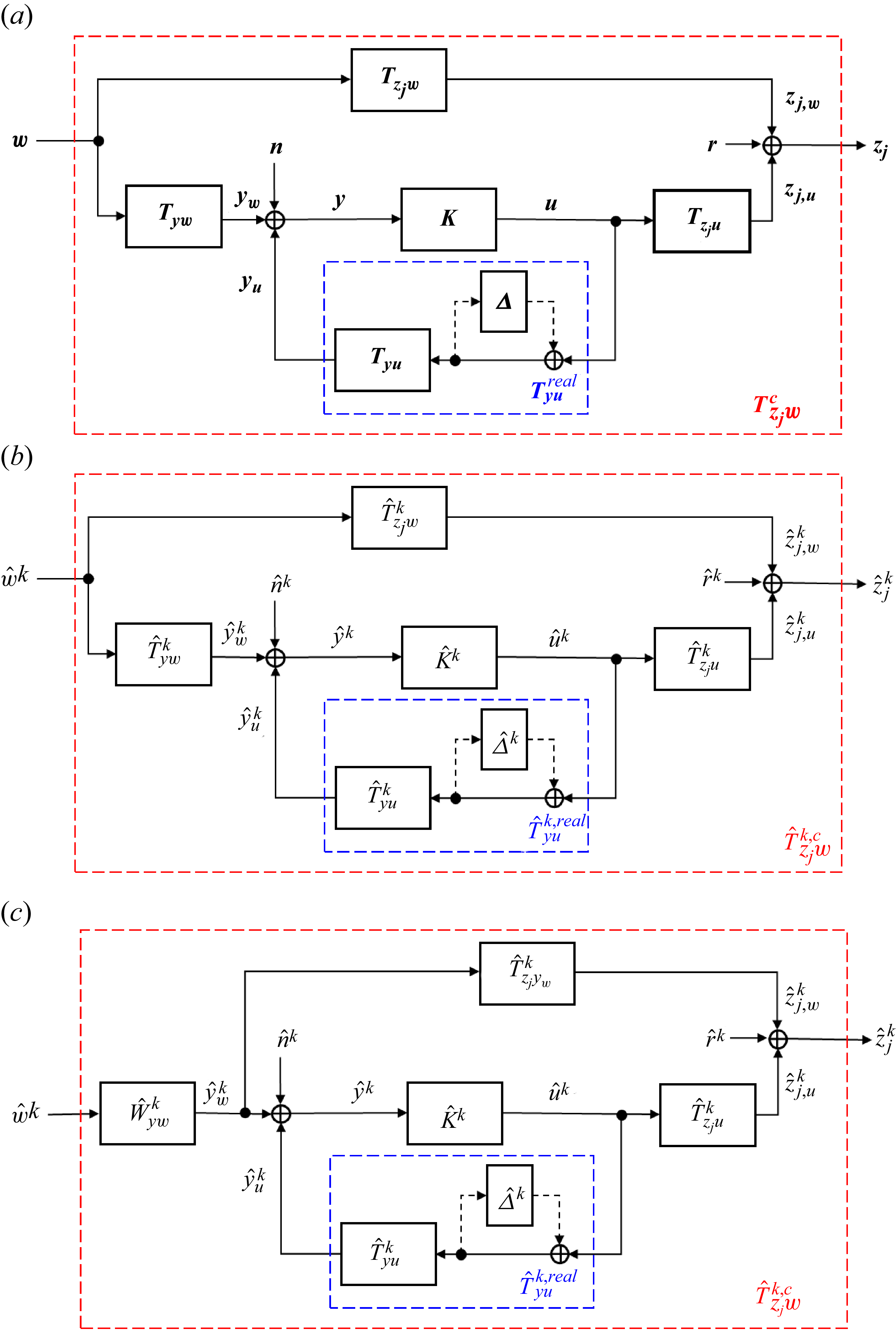
. A block-diagram representation is included in figure 4(a). We also introduce in this block-diagram a measurement noise
 $\boldsymbol{n}$
on the estimation sensors and an example of uncertainty block
 $\boldsymbol{{\varDelta }}$
representing a model error on
 $\boldsymbol{T}_{\!\boldsymbol{yu}}$
; their role and importance will be detailed in § 4.
(a) System representation of the control set-up, including an inverse multiplicative input uncertainty block
 $\boldsymbol{\varDelta }$
and a measurement noise
 $\boldsymbol{n}$
. (b) The
 $n\times n$
centralized MIMO problem of panel (a), with
 $n=2m+1$
may be recast as
 $m+1$
independent single-input–single-output (SISO) problems in the transverse wavenumber space. (c) Introduction of the spectral factor
 $\hat {W}^k_{yw}$
and the Wiener filter
 $\hat {T}^k_{z_{\kern-1pt j}y_w}$
to deal with the unknown input
 $\hat {w}^k$
. This modifies the phase of the closed-loop transfer function, but preserves its module up to a constant scaling factor. Similarly, the performance outputs are redefined as
 $\hat {z}^k_j(t):=\hat {z}^k_j(t+\tau _{\boldsymbol{z}_{\!j}\boldsymbol{y_w}})$
with
 $\tau _{\boldsymbol{z}_{\!j}\boldsymbol{y_w}}$
the convection delay from
 $\boldsymbol{y_w}$
to
 $\boldsymbol{z}_{\!j}$
, without impacting the module of the closed-loop transfer function.
Ignoring
 $\boldsymbol{n}$
and
 $\boldsymbol{\varDelta }$
for now, the closed-loop transfer function from
 $\boldsymbol{w}$
to
 $\boldsymbol{z}_{\!j}$
is
 \begin{align} \boldsymbol{T}_{\!\boldsymbol{z}_{\!j}\boldsymbol{w}}^c=\boldsymbol{T}_{\!\boldsymbol{z}_{\!j}\boldsymbol{w}}+\boldsymbol{T}_{\!\boldsymbol{z}_{\!j}\boldsymbol{u}}\boldsymbol{K}\underbrace {(\boldsymbol{I}-\boldsymbol{T}_{\!\boldsymbol{yu}}\boldsymbol{K})^{-1}}_{\boldsymbol{S}}\boldsymbol{T}_{\!\boldsymbol{yw}}, \end{align}
where
 $\boldsymbol{S}$
is the sensitivity function (Skogestad & Postlethwaite Reference Skogestad and Postlethwaite2005). When designing the controller, we will be concerned with two different norms of the closed-loop transfer function, the classical
 $H_2$
and
 $H_\infty$
norms, subsequently denoted
 $\|(.)\|_2$
and
 $\|(.)\|_\infty$
. The
 $H_2$
norm has the following interpretation in the stochastic framework: if
 $\boldsymbol{w}$
is a white-noise of unit intensity, i.e. of power spectral density (PSD)
 $\boldsymbol{\varPhi }_{\boldsymbol{w}}=\boldsymbol{I}$
, then the
 $H_2$
norm of
 $\boldsymbol{T}^c_{\boldsymbol{z}_{\!j}\boldsymbol{w}}$
provides the standard deviation of
 $\boldsymbol{z}_{\!j}$
at any point in time (in the statistically steady regime), i.e.
 \begin{align} \|\boldsymbol{T}_{\!\boldsymbol{z}_{\!j}\boldsymbol{w}}^c\|_2=\sqrt {E[\|\boldsymbol{z}_{\!j}\|^2]}\quad \text{for }\boldsymbol{\varPhi }_{\boldsymbol{w}}=\boldsymbol{I}, \end{align}
where
 $E[.]$
denotes the expectation. On the other hand, the
 $H_\infty$
norm provides the worst-case amplification of finite-energy perturbations. Denote the time-integrated energy
 $\|\boldsymbol{z}_{\!j} (t)\|_2=\sqrt {\int _0^\infty \|\boldsymbol{z}_{\!j}\|^2\,\mathrm{d}t}$
, then
 \begin{align} \|\boldsymbol{T}_{\!\boldsymbol{z}_{\!j}\boldsymbol{w}}^c\|_\infty =\max _{0\lt \|\boldsymbol{w}(t)\|_2\lt \infty }\dfrac {\|\boldsymbol{z}_{\!j}(t)\|_2}{\|\boldsymbol{w}(t)\|_2}. \end{align}
For stable systems, these norms may be computed as follows:
 \begin{align} \|\boldsymbol{T}\|_2&=\sqrt {\dfrac {1}{2\pi }\int _{-\infty }^\infty \|\boldsymbol{T}(\mathrm{i}\omega )\|^2_{{F}}\,\mathrm{d}\omega },&\text{with }\quad \|\boldsymbol{T}(\mathrm{i}\omega )\|^2_{{F}}&=\mathrm{Tr}(\boldsymbol{T}^H(\mathrm{i}\omega )\boldsymbol{T}(\mathrm{i}\omega )),\nonumber \\ \|\boldsymbol{T}\|_\infty &=\sup _{\omega \in \mathbb{R}}\|\boldsymbol{T}(\mathrm{i}\omega )\|_2,&\text{with }\quad \|\boldsymbol{T}(\mathrm{i}\omega )\|_2&=\bar {\sigma }\left (\boldsymbol{T}(\mathrm{i}\omega )\right ), \end{align}
where
 $\|(.)\|_{{F}}$
denotes the Frobenius norm and
 $\bar {\sigma }(.)$
denotes the largest singular value.
The controller
 $\boldsymbol{K}$
is a full
 $n\times n$
matrix so the control set-up is called centralized. For large values of
 $n$
, designing a structured (i.e. of a given order) controller to minimize the
 $H_2$
/
 $H_\infty$
norms is a challenging task so in the next section, we will exploit the symmetries of the problem in order to decouple the problem into a fully decentralized one.
3.2. Exploiting symmetries
The flow configuration has key symmetries that we wish to exploit. The basic flow has no transverse velocity component, i.e.
 $\bar {v}_{x_3}=0$
, and is invariant in the transverse direction, i.e.
 $\partial _{x_3} \bar {v}_{x_1}=\partial _{x_3} \bar {v}_{x_2}=\partial _{x_3} \bar {p} = \partial _{x_3} \bar {T} = 0$
. The control set-up is periodic in the transverse direction, with period
 $L_{x_3}$
, and flow perturbations about the basic flow are also
 $ L_{x_3}$
-periodic. Furthermore, source and measurement fields consist in arrays of identical fields regularly distributed along the transverse direction, with the same number
 $n$
in one period
 $L_{x_3}$
. The noise–actuator–sensor set-up is therefore periodic with period
 $ L_{x_3}/n=\varDelta _{x_3}$
, even though the flow field is only
 $ L_{x_3}$
-periodic.
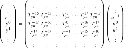
Under these hypotheses, all the previously introduced transfer matrices are circulant. For example,
 ${\boldsymbol{y}}={\boldsymbol{T}}_{\boldsymbol{yu}}{\boldsymbol{u}}$
may be written more explicitly,
 \begin{align} \left (\begin{array}{c} \vdots \\ y^{-1} \\ y^0 \\ y^{1} \\ \vdots \end{array}\right )&= \begin{pmatrix} \vdots & \vdots & \vdots & \vdots & \vdots & \vdots & \vdots \\[5pt] T_{yu}^{-16} & T_{yu}^{-15} & {\cdots} & T_{yu}^{1} & {\cdots} & T_{yu}^{17} & T_{yu}^{-17} \\[5pt] T_{yu}^{-17} & T_{yu}^{-16} & {\cdots} & T_{yu}^{0} & {\cdots} & T_{yu}^{16} & T_{yu}^{17} \\[5pt] T_{yu}^{17} & T_{yu}^{-17} & {\cdots} & T_{yu}^{-1} & {\cdots} & T_{yu}^{15} & T_{yu}^{16} \\[5pt] \vdots & \vdots & \vdots & \vdots & \vdots & \vdots & \vdots \end{pmatrix}\left (\begin{array}{c} \vdots \\ u^{-1} \\ u^0 \\ u^{1} \\ \vdots \end{array}\right )\!, \end{align}
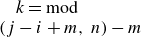
with
 $T_{yu}^{\,k}=T_{y^i u^j}$
(
 $T_{y^i u^j}$
representing the SISO transfer from
 $u^j$
to
 $y^i$
) and
 $k = \mathrm{mod} (j-i+m,\,n)-m$
for all
 $ |i| \leqslant m$
and
 $ |j| \leqslant m$
. Since circulant systems can be expressed as circular discrete convolutions, passing to Fourier space transforms the convolution into a componentwise multiplication, resulting in a diagonal representation of the transfer matrices,
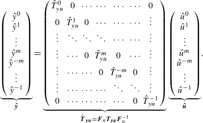 \begin{align} \underbrace {\left (\begin{array}{c} \hat {y}^0 \\ \hat {y}^{1} \\ \vdots \\ \hat {y}^{m} \\ \hat {y}^{-m} \\ \vdots \\ \hat {y}^{-1}\end{array}\right )}_{\boldsymbol{\hat {y}}}&=\underbrace {\left ( \begin{array}{ccccccc} \hat {T}_{yu}^{0} & 0 & {\cdots} & {\cdots} & {\cdots} & {\cdots} & 0 \\ 0 & \hat {T}_{yu}^{1} & 0 & {\cdots} & {\cdots} &{\cdots} & \vdots \\ \vdots & \ddots & \ddots & \ddots & {\cdots} & {\cdots} & \vdots \\ \vdots & {\cdots} & 0 &\hat {T}_{yu}^{m} & 0 & {\cdots} & \vdots \\ \vdots & {\cdots} & {\cdots} & 0 & \hat {T}_{yu}^{-m} & 0 & \vdots \\ \vdots & {\cdots} & {\cdots} & {\cdots} & \ddots & \ddots & \vdots \\ 0 & {\cdots} & {\cdots} & {\cdots} & {\cdots} & 0 & \hat {T}_{yu}^{-1} \end{array} \right )}_{\hat {\boldsymbol{T}}_{\boldsymbol{yu}}=\boldsymbol{F}_n\boldsymbol{T}_{\!\boldsymbol{yu}} \boldsymbol{F}_n^{-1}} \underbrace {\left (\begin{array}{c} \hat {u}^0 \\ \hat {u}^{1} \\ \vdots \\ \hat {u}^{m} \\ \hat {u}^{-m} \\ \vdots \\ \hat {u}^{-1}\end{array}\right )}_{\boldsymbol{\hat {u}}}, \end{align}
where
 $\boldsymbol{\hat {y}}=\boldsymbol{F}_n \boldsymbol{{y}}$
denotes the discrete Fourier transform (DFT) of vector
 $\boldsymbol{{y}}$
(and similarly for
 $\boldsymbol{w}$
,
 $\boldsymbol{u}$
and
 $\boldsymbol{z}$
), the matrix
 $ \boldsymbol{F}_n$
being the unitary DFT matrix defined by
 $(F_n)_{ki}=n^{-1/2}\omega _n^{ki}$
for
 $k,i=0,\ldots, n-1$
and satisfying
 $\boldsymbol{F}_n\boldsymbol{F}_n^H=\boldsymbol{F}_n^H\boldsymbol{F}_n=\boldsymbol{I}$
. Here
 $(.)^H$
denotes the Hermitian conjugate, and
 $\omega _n=\mathrm{e}^{-{i}2\pi /n}$
is the primitive nth root of unity. Hence, each
 $\hat {T}_{yu}^{k}$
represents the transfer function associated with the
 $k^{th}$
spanwise Fourier mode of
 $\boldsymbol{{y}}$
and
 $\boldsymbol{{u}}$
. The kth spanwise mode corresponds to a non-dimensional transverse wavenumber
 $(k\beta /n)\delta _0^*$
, where
 $\beta = 2\pi /\varDelta _{x_3}$
is the wavenumber associated with the distance
 $\varDelta _{x_3}$
between two consecutive sensors/actuators in
 $x_3$
-direction.
The DFT matrix being unitary, we have (Parseval)
 \begin{align} \|\hat {\boldsymbol{T}}_{\boldsymbol{y}\boldsymbol{u}}(\mathrm{i}\omega )\|_{{F}}=\|\boldsymbol{T}_{\!\boldsymbol{y}\boldsymbol{u}}(\mathrm{i}\omega )\|_{{F}}&\quad \Rightarrow \quad \|\hat {\boldsymbol{T}}_{\boldsymbol{y}\boldsymbol{u}}\|_2=\|\boldsymbol{T}_{\!\boldsymbol{y}\boldsymbol{u}}\|_2,\nonumber \\ \|\hat {\boldsymbol{T}}_{\boldsymbol{y}\boldsymbol{u}}(\mathrm{i}\omega )\|_{2}=\|\boldsymbol{T}_{\!\boldsymbol{y}\boldsymbol{u}}(\mathrm{i}\omega )\|_{2}&\quad \Rightarrow \quad \|\hat {\boldsymbol{T}}_{\boldsymbol{y}\boldsymbol{u}}\|_\infty =\|\boldsymbol{T}_{\!\boldsymbol{y}\boldsymbol{u}}\|_\infty . \end{align}
Finally,
 $\hat {\boldsymbol{T}}_{\boldsymbol{y}\boldsymbol{u}}$
being diagonal, we have
 \begin{align} \|\hat {\boldsymbol{T}}_{\boldsymbol{y}\boldsymbol{u}}(\mathrm{i}\omega )\|^2_{{F}}=\sum _k |\hat {T}^k_{yu}(\mathrm{i}\omega )|^2 & \quad \Rightarrow \quad \|\hat {\boldsymbol{T}}_{\boldsymbol{y}\boldsymbol{u}}\|^2_2=\sum _k \|\hat {T}^k_{yu}\|_2^2,\nonumber \\ \|\hat {\boldsymbol{T}}_{\boldsymbol{y}\boldsymbol{u}}(\mathrm{i}\omega )\|_2=\max _k |\hat {T}^k_{yu}(\mathrm{i}\omega )| & \quad \Rightarrow \quad \|\hat {\boldsymbol{T}}_{\boldsymbol{y}\boldsymbol{u}}\|_{\infty }=\max _k \|\hat {T}^k_{yu}\|_\infty . \end{align}
Therefore, minimizing the
 $H_2$
or the
 $H_\infty$
norm for each integer
 $k$
independently results in the minimization of the
 $H_2$
or
 $H_\infty$
norm of the full system. By exploiting the symmetries of our set-up, we convert a
 $n\times n$
centralized MIMO problem into a decentralized MIMO problem made of
 $n$
SISO subproblems, represented in figure 4(b). The closed-loop transfer function for each integer
 $-m\leqslant k\leqslant m$
is
 \begin{align} \hat {T}^{k,c}_{z_{\kern-1pt j}w}=\hat {T}^k_{z_{\kern-1pt j}w}+\hat {T}^k_{z_{\kern-1pt j}u}\hat {K}^k\underbrace {\big(1-\hat {T}^k_{yu}\hat {K}^k \big)^{-1}}_{\hat {S}^k}\hat {T}^k_{yw}. \end{align}
The SISO block diagram is similar to the one introduced in Nibourel et al. (Reference Nibourel, Leclercq, Demourant, Garnier and Sipp2023) for the case of spanwise invariant perturbations, so we may use the same approach for synthesis. One difference with the 2-D case though is that the input and output variables are now complex in the time-domain. This is not an issue here because the impulse responses associated with the complex input–output pairs are real in our case (see Appendix B), therefore system identification of controller synthesis may be performed in Fourier space, using real algebra, exactly as in Nibourel et al. (Reference Nibourel, Leclercq, Demourant, Garnier and Sipp2023). Moreover, all transfer functions satisfy the symmetry
 \begin{align} \hat {T}^{-k}=\hat {T}^k \end{align}
(see Appendix B), therefore we only need to perform identification and synthesis for the
 $m+1$
transverse wavenumbers
 $k=0,\ldots, m$
.
Each controller
 $\hat {K}^k$
is synthesized independently in state-space form
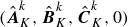 $(\hat {\boldsymbol{A}}_K^k,\hat {\boldsymbol{B}}_K^k,\hat {\boldsymbol{C}}_K^k,0)$
where
 $\hat {\boldsymbol{A}}_K^k$
,
 $\hat {\boldsymbol{B}}_K^k$
and
 $\hat {\boldsymbol{C}}_K^k$
denote the state, input and output matrices (Skogestad & Postlethwaite Reference Skogestad and Postlethwaite2005) of the controller associated with mode
 $k$
. As long as the perturbations remain within the linear regime, each spanwise mode
 $k$
evolve independently and consequently, each controller
 $\hat {K}^k$
operates independently. A real state-space representation of the total controller
 $\boldsymbol{K}$
is then retrieved as
 $(\hat {\boldsymbol{A}}_K,\hat {\boldsymbol{B}}_K\boldsymbol{F}_n,\boldsymbol{F}_n^{-1}\hat {\boldsymbol{C}}_K,0)$
, where
 $\hat {\boldsymbol{A}}_K=\mathrm{blkdiag}(\hat {\boldsymbol{A}}_K^0,\ldots, \hat {\boldsymbol{A}}_K^m,\hat {\boldsymbol{A}}_K^m,\ldots, \hat {\boldsymbol{A}}_K^1)$
,
 $\hat {\boldsymbol{B}}_K=\mathrm{blkdiag}(\hat {\boldsymbol{B}}_K^0,\ldots, \hat {\boldsymbol{B}}_K^m,\hat {\boldsymbol{B}}_K^m,\ldots, \hat {\boldsymbol{B}}_K^1)$
and
 $\hat {\boldsymbol{C}}_K=\mathrm{blkdiag}(\hat {\boldsymbol{C}}_K^0,\ldots, \hat {\boldsymbol{C}}_K^m,\hat {\boldsymbol{C}}_K^m,\ldots, \hat {\boldsymbol{C}}_K^1)$
. The matrices
 $\hat {\boldsymbol{B}}_K\boldsymbol{F}_n$
and
 $\boldsymbol{F}_n^{-1}\hat {\boldsymbol{C}}_K$
are real indeed because of the symmetry
 $\hat {\boldsymbol{B}}^{-k}_K=\hat {\boldsymbol{B}}^k_K$
and
 $\hat {\boldsymbol{C}}^{-k}_K=\hat {\boldsymbol{C}}^k_K$
. The total controller
 $\boldsymbol{K}$
is the one implemented in the computational fluid dynamics (CFD) solver FastS for the closed-loop simulations: the control signal vector
 $\boldsymbol{u}$
is updated from the estimation signal vector
 $\boldsymbol{y}$
by solving the first-order differential equations of the controller state-space representation (Nibourel et al. Reference Nibourel, Leclercq, Demourant, Garnier and Sipp2023, Reference Nibourel, Leclercq, Demourant, Garnier and Sipp2024).
3.3. Dealing with the unknown input
 $\boldsymbol{w}$

The SISO transfer functions
 $\hat {T}^k_{yu}$
and
 $\hat {T}^k_{z_{\kern-1pt j}u}$
may be identified from input–output data as we shall see in § 6.1, however, this is not possible for
 $\hat {T}^k_{yw}$
and
 $\hat {T}^k_{z_{\kern-1pt j}w}$
, because the exogenous noise
 $\boldsymbol{w}$
cannot be measured in a realistic set-up. First we introduce a Wiener filter
 $\hat {T}^k_{z_{\kern-1pt j} y_w}$
(Sasaki et al. Reference Sasaki, Morra, Fabbiane, Cavalieri, Hanifi and Henningson2018, Reference Sasaki, Morra, Cavalieri, Hanifi and Henningson2020; Morra et al. Reference Morra, Sasaki, Hanifi, Cavalieri and Henningson2020) to optimally estimate
 $\hat {z}_{j,w}^k$
from
 $\hat {y}_w^k$
(estimation measurements in absence of control). As a result
 \begin{align} \hat {z}^k_{j,w}=\hat {T}^k_{z_{\kern-1pt j} y_w}\hat {y}_w^k+\hat {r}^k, \end{align}
where
 $\hat {r}^k$
is a residual due to the fact that some information measured by
 $\hat {z}_{j,w}^k$
is missing in
 $\hat {y}_w^k$
(e.g. nonlinearities, noise on performance sensors, spectral leakage, linear contributions from other unmeasured inputs, etc.) (Bendat & Piersol Reference Bendat and Piersol1971; Morra et al. Reference Morra, Sasaki, Hanifi, Cavalieri and Henningson2020). Because sensors
 $\boldsymbol{y}$
are far upstream of
 $\boldsymbol{z}_{\!j}$
, there are no specific precautions to take with respect to causality and the simple formula
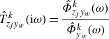 \begin{align} \hat {T}^k_{z_{\kern-1pt j}y_w}(\mathrm{i}\omega )=\dfrac {\hat {\varPhi }_{z_{\kern-1pt j}y_w}^k(\omega )}{\hat {\varPhi }_{y_w}^k(\omega )} \end{align}
provides the frequency response of the optimal causal filter (Glad & Ljung Reference Glad and Ljung2000). Both spectral and cross-spectral power densities
 $\hat {\varPhi }^k(\omega )$
may be estimated from data with actuation switched off. Using the filter, we may write
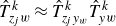 \begin{align} \hat {T}^k_{z_{\kern-1pt j}w}\approx \hat {T}^k_{z_{\kern-1pt j}y_w}\hat {T}^k_{yw} \end{align}
which leads, using (3.18), to
 \begin{align} \hat {T}^{k,c}_{z_{\kern-1pt j}w}\approx \big(\hat {T}^k_{z_{\kern-1pt j}y_w}+\hat {T}^k_{z_{\kern-1pt j}u}\hat {K}^k\hat {S}^k \big)\hat {T}^k_{yw}. \end{align}
Optimizing the
 $H_2$
or
 $H_\infty$
norm only requires the computation of the module of
 $\hat {T}^{k,c}_{z_{\kern-1pt j}w}$
, therefore, the phase information of
 $\hat {T}^k_{yw}$
is irrelevant. The module of
 $\hat {T}^k_{yw}$
satisfies
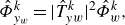 \begin{align} \hat {\varPhi }^k_{y_w}=|\hat {T}^k_{yw}|^2\hat {\varPhi }^k_w, \end{align}
where, again, the spectral density
 $\hat {\varPhi }^k_{y_w}$
of
 $\hat {y}^k_w$
can be measured. Without loss of generality, we may assume that
 $\boldsymbol{w}$
is a white-noise, and we introduce
 $\hat {W}^k_{yw}$
as a spectral factor of
 $\hat {\varPhi }^k_{y_w}$
. Hence
 $\hat {W}^k_{yw}$
is just a stable and causal filter, whose inverse is also a stable and causal filter, such that
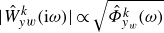 $|\hat {W}^k_{yw}(\mathrm{i}\omega )|\propto \sqrt {\hat {\varPhi }^k_{y_w}(\omega )}$
for all frequencies. The weighting function
 $\hat {W}^k_{yw}$
is not unique, being defined up to an arbitrary phase and scaling factor in magnitude, which do not affect the synthesis step due to
 $H_2/H_{\infty }$
minimization. This leads to the final equation,
 \begin{align} \hat {T}^{k,c}_{z_{\kern-1pt j}w}\approx \big(\hat {T}^k_{z_{\kern-1pt j}y_w}+\hat {T}^k_{z_{\kern-1pt j}u}\hat {K}^k\hat {S}^k \big)\hat {W}^k_{yw}, \end{align}
where all the SISO transfer functions may be identified from input–output data in an experimental configuration. The block diagram involving the Wiener filter and the spectral factor is represented in figure 4(c): it represents the closed-loop transfer function, up to a negligible phase error and magnitude scaling factor both due to
 $\hat {W}_{yw}^k$
, and up to the residual error
 $\hat {r}^k$
of (3.20) from the Wiener filter.
3.4. Dealing with delays
When introducing the spectral factor
 $\hat {W}^k_{yw}$
, we discussed the fact that introducing an error in the phase of the closed-loop transfer function has no impact on controller synthesis, because system norms are only concerned with
 $|\hat {T}^{k,c}_{z_{\kern-1pt j} w}|$
. We may exploit this property once again by swapping the performance sensors
 $\boldsymbol{z}_{\!j}(t)$
with the non-causal sensors
 \begin{align} \boldsymbol{z}_{\!j}(t):=\boldsymbol{z}_{\!j}(t+\tau _{\boldsymbol{z}_{\!j}\boldsymbol{y_w}}), \end{align}
where
 $\tau _{\boldsymbol{z}_{\!j}\boldsymbol{y_w}}\gt 0$
is the convection delay from
 $\boldsymbol{y_w}$
to
 $\boldsymbol{z}_{\!j}$
. This procedure has already been used in Nibourel et al. (Reference Nibourel, Leclercq, Demourant, Garnier and Sipp2023, Reference Nibourel, Leclercq, Demourant, Garnier and Sipp2024). The fact that the new sensors are not causal is not problematic because performance sensors do not need to implemented in real-time, they only serve for the controller synthesis step, which is performed offline. Translating the
 $\boldsymbol{z}_{\!j}$
signals backward in time amounts to multiplying the transfer functions
 $\hat {T}^k_{z_{\kern-1pt j} y_w}$
and
 $\hat {T}^k_{z_{\kern-1pt j} u}$
by the non-causal filter
 $\mathrm{e}^{s\tau _{\boldsymbol{z}_{\!j}\boldsymbol{y_w}}}$
. By examining (3.25), we see that this filter factors out and therefore applies to the full closed-loop transfer function. Since the frequency response of the filter has a constant module equal to unity, the module of the frequency response of the closed-loop transfer function remains unchanged. This procedure leads to no loss of information because even though the filter
 $\mathrm{e}^{s\tau _{\boldsymbol{z}_{\!j}\boldsymbol{y_w}}}$
is non-causal, the shifted frequency responses from
 $\boldsymbol{u}$
and
 $\boldsymbol{y_w}$
to
 $\boldsymbol{z}_{\!j}$
remain causal, so no information is ‘lost in the past’ during the system identification step. Indeed, between
 $0\leqslant t\leqslant \tau _{\boldsymbol{z}_{\!j}\boldsymbol{y_w}}$
, both impulse responses are zero, because perturbations did not have time to reach
 $\boldsymbol{z}_{\!j}$
yet. We may therefore safely discard the initial deadtime
 $\tau _{\boldsymbol{z}_{\!j}\boldsymbol{y_w}}$
from both impulse responses without affecting the closed-loop system norm. This procedure has great benefits for both system identification and controller synthesis, because the lower the time-delay, the lower the order of the corresponding state-space representation and the cheaper controller synthesis. Note that we may not remove the deadtime from
 $\boldsymbol{u}$
to
 $\boldsymbol{y}$
without artificially changing the closed-loop dynamics, so this deadtime must remain.
3.5. Defining the number of sensors and actuators
In this section, we start by assuming that the number of sensors
 $n_y$
and
 $n_z$
and the number of actuators
 $n_u$
, per unit length
 $L_{x_3}$
, may take different values. Noise sources are infinitely localized along the transverse direction
 $x_3$
so they excite all transverse Fourier modes equally. The smallest wavelengths are filtered by viscosity and at the sensor positions there are minimum wavelengths
 $\lambda _{\textit{min}}^{\boldsymbol{y_w}}$
and
 $\lambda _{\textit{min}}^{\boldsymbol{z}_{j,\boldsymbol{w}}}$
containing energy in the signals
 $\boldsymbol{y_w}$
and
 $\boldsymbol{z}_{j,\boldsymbol{w}}$
(the signals of
 $\boldsymbol{y}$
and
 $\boldsymbol{z}_{\!j}$
when excited only by the exogenous noises
 $\boldsymbol{w}$
), respectively. The minimum wavelengths containing energy in the signals
 $\boldsymbol{y_u}$
and
 $\boldsymbol{z}_{j,\boldsymbol{u}}$
(the signals of
 $\boldsymbol{y}$
and
 $\boldsymbol{z}_{\!j}$
when excited only by the actuators
 $\boldsymbol{u}$
) are, in the linear regime, greater than
 $\lambda _{\textit{min}}^{b_u}$
, the minimum wavelength in the spectrum (in space) of the actuator field
 $b_u(x_3)$
. To avoid aliasing, the number of sensors must satisfy
 \begin{align} n_y\geqslant 2\dfrac {L_{x_3}}{\min \big(\lambda _{\textit{min}}^{\boldsymbol{y_w}},\lambda _{\textit{min}}^{b_u} \big)},\quad n_z\geqslant 2\dfrac {L_{x_3}}{\min \big(\lambda _{\textit{min}}^{\boldsymbol{z}_{j,\boldsymbol{w}}},\lambda _{\textit{min}}^{b_u} \big)}. \end{align}
As long as the dynamics is linear, it is also expected that
 $\lambda _{\textit{min}}^{\boldsymbol{z}_{j,\boldsymbol{w}}}\geqslant \lambda _{\textit{min}}^{\boldsymbol{y_w}}$
, as small structures are damped as they propagate downstream. On the other hand, if transition begins upstream of both sets of sensors, the opposite is true, but we exclude that scenario in the present paper.
The number of observable transverse Fourier modes is equal to the number of sensors, i.e.
 $n_y$
and
 $n_z$
. Similarly, the number of controllable Fourier modes is equal to the number of actuators
 $n_u$
. If
 $n_y$
is too small, then aliasing occurs and results in measurement noise on the observable modes. Similarly, we need
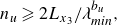 \begin{align} n_u\geqslant 2L_{x_3}/\lambda _{\textit{min}}^{b_u}, \end{align}
otherwise actuation noise related to uncontrollable modes is introduced. In the linear limit, this actuation noise can be completely filtered out by the measurement if inequalities (3.27) are satisfied, so the closed-loop is not affected for the
 $n_u$
controllable modes (it goes without saying that
 $n_u\leqslant \min (n_y,n_z)$
). However, this actuation noise can affect the nonlinear dynamics and negatively impact transition to turbulence. Thus, to minimize the number of sensors and actuators while avoiding the problems of measurement and actuation noise, it is desirable to choose actuators whose support is such that
 $\lambda _{\textit{min}}^{b_u}\geqslant \lambda _{\textit{min}}^{\boldsymbol{y_w}}$
, to choose a common number
 $n=n_u=n_y=n_z$
of actuators/sensors, and verify the condition
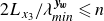 $ 2L_{x_3}/\lambda _{\textit{min}}^{\boldsymbol{y_w}}\leqslant n$
. In this paper we choose
 $n=35$
, which, as we shall see, is more than enough.
4. Robust control specifications
For each wavenumber
 $k$
, the control objective is to design a control law
 $\hat {K}^k$
reducing as much as possible amplitude disturbances, while ensuring efficiency and stability despite modelling errors, unmodeled noise sources or variations in inflow conditions. In this section, these fluid specifications are reinterpreted from a control perspective (i.e. constraints/reductions of
 $H_\infty /H_2$
norms of closed-loop transfer functions), enabling the introduction of key robust control principles: nominal performance/stability, robust stability and robust performance.
4.1. Nominal performance/stability
In this study, the concept of nominal performance focuses to noise cancellation, in order to delay the laminar-to-turbulent transition, which occurs once a critical amplitude threshold is exceeded. Hence, the lower the ratio
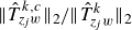 $\|\hat {T}^{k,c}_{z_{\kern-1pt j}w}\|_2/\|\hat {T}^{k}_{z_{\kern-1pt j}w}\|_2$
in nominal point condition (i.e. no uncertainties, errors or variations in the modelled transfer functions are considered), the better the nominal performance. One might also ask what is the most effective set-up for delaying transition between minimizing
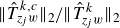 $\|\hat {T}^{k,c}_{z_{\kern-1pt j}w}\|_2/\|\hat {T}^{k}_{z_{\kern-1pt j}w}\|_2$
or
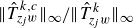 $\|\hat {T}^{k,c}_{z_{\kern-1pt j}w}\|_\infty /\|\hat {T}^{k}_{z_{\kern-1pt j}w}\|_\infty$
but this is considered beyond the scope of the current study.
Concerning the concept of nominal stability, it refers to the requirement that the closed-loop system, built from the nominal model
 $\hat {T}^k_{yu}$
and the designed controller
 $\hat {K}^k$
, is stable in the absence of uncertainty. Since
 $-\hat {T}^k_{yu}\hat {K}^k$
does not exhibit any unstable pole (
 $\hat {T}^k_{yu}$
is stable because the boundary layer flow is globally stable, while
 $\hat {K}^k$
is stable by design), the closed-loop system is stable if and only if the Nyquist plot of
 $-\hat {T}^k_{yu}\hat {K}^k$
does not encircle the critical point (−1,0). This notion of nominal stability (Skogestad & Postlethwaite Reference Skogestad and Postlethwaite2005) is meaningful only in a feedback configuration (feedforward control is unconditionally stable as
 $\hat {T}^k_{yu}=0$
) and serves as the foundational prerequisite for subsequent analyses of robust stability.
4.2. Robust stability
Robust stability concerns the preservation of closed-loop stability when the true plant
 $\hat {T}^{k,\textit{real}}_{yu}$
deviates from its nominal model
 $\hat {T}^k_{yu}$
within a class of uncertainty
 $\hat {\varDelta }^k$
. The uncertain plant can be expressed as the feedback interconnection of a stable closed-loop transfer operator
 $\hat {M}^k$
with the norm-bounded stable uncertainty
 $\hat {\varDelta }^k$
. The small gain theorem (Zames Reference Zames1966; Skogestad & Postlethwaite Reference Skogestad and Postlethwaite2005) then yields a necessary and sufficient condition for robust stability,
 \begin{align} \|\hat {M}^k\hat {\varDelta }^k\|_\infty \lt 1. \end{align}
Indeed, ensuring this
 $H_\infty$
criterion guarantees that the Nyquist curve of the uncertain loop cannot be displaced so as to encircle the critical point, thereby preserving stability (Skogestad & Postlethwaite Reference Skogestad and Postlethwaite2005).
In the case where the real system can be expressed as
 \begin{align} \hat {T}_{yu}^{k,\textit{real}}=\frac {\hat {T}^k_{yu}}{1-\hat {\varDelta }^k} \quad \Leftrightarrow \quad \hat {\varDelta }^k=\frac {\hat {T}_{yu}^{k,\textit{real}}-\hat {T}^k_{yu}}{\hat {T}_{yu}^{k,\textit{real}}}, \end{align}
the operator
 $\hat {\varDelta }^k$
is referred to as an inverse multiplicative uncertainty (see in figure 4). This type of uncertainty is often preferred, as it can be naturally interpreted as a relative modelling error. The requirement that
 $-\hat {T}_{yu}^{k,\textit{real}}K$
does not encircle the critical point (−1,0) is then equivalent to satisfying the condition (Skogestad & Postlethwaite Reference Skogestad and Postlethwaite2005)
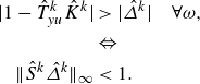 \begin{align} |1-\hat {T}^k_{yu}\hat {K}^k|&\gt |\hat {\varDelta }^k| \quad \forall \omega, \nonumber \\ &\Leftrightarrow \nonumber \\ \|\hat {S}^k\hat {\varDelta }^k\|_{\infty }&\lt 1. \end{align}
Therefore, from a control point of view, imposing this
 $H_{ \infty }$
constraint guarantees the internal stability of the closed-loop up to a value
 $\hat {\varDelta }^k$
of relative model error on
 $\hat {T}^k_{yu}$
. Nevertheless, this type of multiplicative uncertainty has two limitations. The first is that it is only meaningful within the system’s bandwidth; outside this range, the very low values of
 $\hat {T}^{k,\textit{real}}_{yu}$
render the multiplicative uncertainty ill-conditioned. The second limitation is that for non-minimum phase systems (Skogestad & Postlethwaite Reference Skogestad and Postlethwaite2005) such as noise-amplifier flows,
 $\hat {\varDelta }^k$
is often unstable or non-causal unless special precautions are taken during its construction, making the classical small-gain criterion inapplicable. Consequently, multiplicative uncertainties account only for uncertainties that can be represented, for example, such as the worst-case combination of pure gain and pure phase shifts (so the most generic measure of available stability margin), representing in our case growth rate and convection speed estimation errors, respectively.
In order to address the shortcomings of multiplicative uncertainty, it is often convenient to also introduce an additive uncertainty,
 \begin{align} \hat {\varDelta }^k=\hat {T}_{yu}^{k,\textit{real}}-\hat {T}^k_{yu}. \end{align}
Indeed, additive uncertainty allows one to capture a broad range of model discrepancies while ensuring that
 $\hat {\varDelta }^k$
remains stable for boundary layer flows. Moreover, additive uncertainty is particularly well-suited for modelling discrepancies outside the system’s bandwidth, where multiplicative uncertainty would otherwise result in an ill-conditioned ratio. Hence, this additive uncertainty framework is therefore more general than the multiplicative framework, albeit at the cost of being more conservative within the bandwidth of interest (Skogestad & Postlethwaite Reference Skogestad and Postlethwaite2005). For the additive uncertainty
 $\hat {\varDelta }^k$
, the Nyquist stability requirement that
 $-\hat {T}_{yu}^{k,\textit{real}}K$
does not encircle the critical point (−1,0) is then equivalent to satisfying the condition
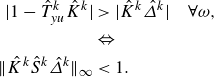 \begin{align} |1-\hat {T}^k_{yu}\hat {K}^k|&\gt |\hat {K}^k\hat {\varDelta }^k| \quad \forall \omega, \nonumber \\ &\Leftrightarrow \nonumber \\ \|\hat {K}^k\hat {S}^k\hat {\varDelta }^k\|_{\infty }&\lt 1. \end{align}
In summary, robust stability for boundary-layer flows can be addressed by shaping both
 $\hat {S}^k$
and
 $\hat {K}^k\hat {S}^k$
. While
 $\hat {S}^k$
captures only specific, well-defined uncertainties within the bandwidth – such as pure gain or phase shifts –
 $\hat {K}^k\hat {S}^k$
accounts for more general discrepancies, particularly outside the bandwidth where the nominal plant has low gain.
4.3. Robust performance
The concept of robust performance consists here in maintaining performance in terms of amplitude reduction despite differences between on-design and off-design operating conditions: the lower the ratio
 $\|\hat {T}^{k,c}_{z_{\kern-1pt j}w}\|_2$
/
 $\|\hat {T}^{k}_{z_{\kern-1pt j}w}\|_2$
despite for example free stream variations, new noise sources or nonlinearities, the better the performance robustness. Note that only model flaws on
 $\hat {T}_{yu}^k$
, which lies within the feedback loop, can lead to instability; uncertainties on other transfers outside the loop (e.g.
 $\hat {T}^k_{z_{\kern-1pt j}u}$
,
 $\hat {T}^k_{z_{\kern-1pt j}y_w}$
,
 $\hat {W}^k_{yw}$
) merely degrade performance without compromising stability.
In case of maintaining performance when free stream condition variations are considered, using a feedback control structure (instead of a feedforward one) designed for the nominal operating point may be sufficient provided that the variations around this point are not too large (Nibourel et al. Reference Nibourel, Leclercq, Demourant, Garnier and Sipp2023, Reference Nibourel, Leclercq, Demourant, Garnier and Sipp2024). In such cases of free stream uncertainties, it may not be necessary to constrain other transfer functions in the synthesis step and just the natural ability of the feedback to handle modelling errors is sufficient to ensure robust performance.
In case of new noise source
 $\hat {n}^k$
modelling a noise measurement on the estimation sensor (displayed in figure 4), a common practice is to constrain
 $\hat {K}^k\hat {S}^k$
to limit the actuator activity on certain bandwidth. Indeed, the quantity
 $\hat {K}^k\hat {S}^k$
may represent the transfer from noise
 $\hat {n}^k$
(corrupting
 $\hat {y}^k$
) to
 $\hat {u}^k$
. To desensitize
 $\hat {u}^k$
to noisy measurements, one can seek to reduce
 $\|\hat {K}^k\hat {S}^k\|_2$
as this means reducing the root-mean-square (r.m.s.) value of
 $\hat {u}^k(t)$
(i.e. the power spent by the control) in case of white noise
 $\hat {n}^k$
on estimation sensors
 $\hat {y}^k$
. Minimizing
 $\|\hat {K}^k\hat {S}^k\|_2$
appears as the most general way to limit actuator activity when the noise
 $\hat {n}^k$
is unknown; if one seeks to desensitize the controller on a particular frequency range (see e.g. Nibourel et al. Reference Nibourel, Leclercq, Demourant, Garnier and Sipp2023, Reference Nibourel, Leclercq, Demourant, Garnier and Sipp2024) or if the properties of
 $\hat {n}^k$
(e.g. frequency spectrum) are known, it may be of interest to constrain
 $\|\hat {K}^k\hat {S}^k\|_\infty$
. It is worth noting that the same transfer, here
 $\hat {K}^k\hat {S}^k$
, can be associated with both robust stability and robust performance, depending on the source of uncertainty. In the specific case of a new noise source
 $\hat {n}^k$
, the perturbation cannot destabilize the closed loop, since it is uncorrelated with the input–output dynamics. Its effect is therefore purely related to performance. By contrast, modelling errors that directly affect the feedback loop via
 $\hat {T}_{yu}^k$
can compromise both performance and stability, as they alter the closed-loop dynamics themselves.
Nonlinearities can also be viewed through the lens of robust performance, as they may degrade control objectives. However, since the present study uses classical tools of control theory which are mathematically well-established in a linear framework, nonlinear effects cannot be explicitly incorporated in the synthesis step and can only be assessed a posteriori, by evaluating their impact on the achieved performance.
5. Uncontrolled and open-loop dynamics
In this section, we examine the uncontrolled and open-loop dynamics, which helps justifying the various specifications for closed-loop control, including the choice of sensors for the selected actuators.
5.1. Uncontrolled flow
The evolution of the velocity wave packet at the generalized inflection point
 $x_{2,\textit{GIP}}$
and the pressure wave packet near the wall, both generated by an impulse of
 $w^0$
(the exogenous noise source at the centre spanwise position of the domain, see figure 1) is plotted in figure 5. Both wave packets are convected downstream with the same group velocity of approximately
 $0.92V_{\infty }$
and grow in amplitude. Additionally, both wave packets spread in the streamwise and spanwise directions and each wave packet is symmetrical with respect to the spanwise position
 $x_3=0$
(this is consistent with the symmetry (3.19) between transfer functions justified in Appendix B). The two wave packets have different 2-D structure. As the amplification rates of the first mode and second mode are, respectively, maximal for oblique and 2-D perturbations (Mack Reference Mack1984), the velocity wave packet at
 $x_{2,\textit{GIP}}$
and the pressure wave packet near the wall can be associated with the first and second instability modes, respectively. This assumption is justified in more detail in the following.
(a,b,c) Velocity and (d,e,f) pressure wave packets at times
 $tV_{\infty }/\delta _{0}^{*}=$
(a,d)
 $455$
, (b,e)
 $834$
and (c,f)
 $1365$
, generated by an impulse of the exogenous input
 $w^0$
at time
 $t=0$
. The velocity and pressure wave packets are at
 $x_{2,\textit{GIP}}$
and
 $x_2=1.99\delta _0 ^*$
, respectively.
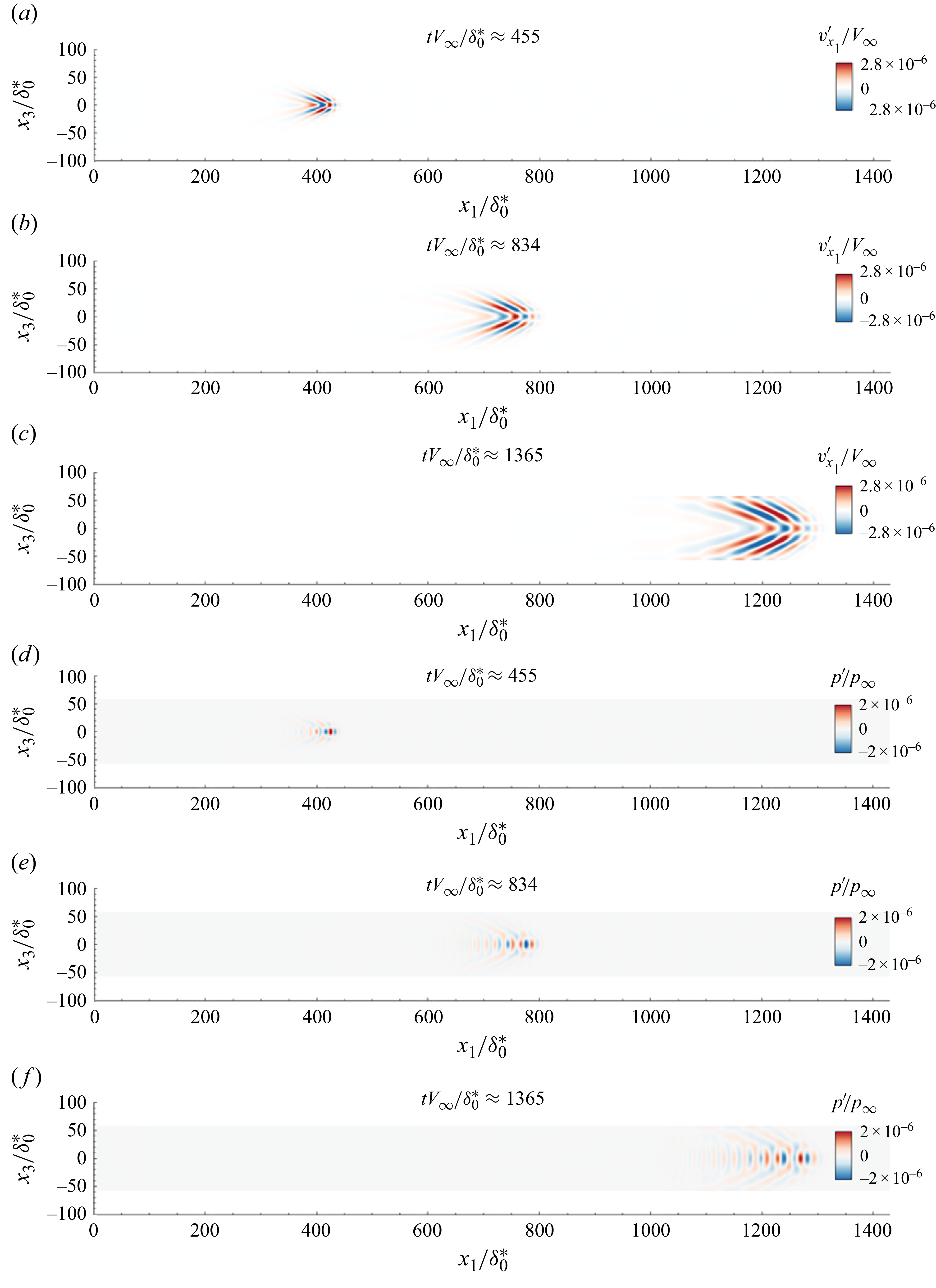
Figure 5. Long description
Panel A: A scatter plot shows velocity wave packets at a normalized time of approximately 455. The x-axis represents the normalized streamwise position, and the y-axis represents the normalized wall-normal position. The color scale indicates the normalized streamwise velocity fluctuation, with red representing positive values and blue representing negative values. The wave packet appears as a concentrated cluster of points around the streamwise position of 400 and wall-normal position of 0. Panel B: Another scatter plot shows velocity wave packets at a normalized time of approximately 834. The axes and color scale are the same as in Panel A. The wave packet has spread out more along the streamwise direction compared to Panel A. Panel C: A scatter plot shows velocity wave packets at a normalized time of approximately 1365. The axes and color scale are the same as in previous panels. The wave packet has further spread out and shows a more elongated shape along the streamwise direction. Panel D: A scatter plot shows pressure wave packets at a normalized time of approximately 455. The x-axis represents the normalized streamwise position, and the y-axis represents the normalized wall-normal position. The color scale indicates the normalized pressure fluctuation, with red representing positive values and blue representing negative values. The wave packet appears as a concentrated cluster of points around the streamwise position of 400 and wall-normal position of 0. Panel E: Another scatter plot shows pressure wave packets at a normalized time of approximately 834. The axes and color scale are the same as in Panel D. The wave packet has spread out more along the streamwise direction compared to Panel D. Panel F: A scatter plot shows pressure wave packets at a normalized time of approximately 1365. The axes and color scale are the same as in previous panels. The wave packet has further spread out and shows a more elongated shape along the streamwise direction.
Linearized DNS is also performed with white-noise from all
 $35$
uncorrelated sources
 $w^i$
. The profiles at
 $x_1=1766.7\delta _0^{*}$
of the r.m.s. fluctuations averaged in the spanwise direction are plotted in figure 6(a). The greatest fluctuations are for thermodynamic quantities (density and temperature fluctuations) which peak near the generalized inflection point (dashed line); the velocity profile also takes its highest value close to
 $x_{2,\textit{GIP}}$
, while the pressure profile has two peaks: the highest one at the wall and a second one at
 $x_{2,\textit{GIP}}$
. These results for the position of the profile peaks at
 $x_1=1766.7\delta _0^{*}$
are true for all streamwise positions (see figure 6
b). Note that upstream of the domain, the pressure maxima in the wall-normal direction are not at the wall; external noise sources generate an acoustic wave leaving the boundary layer. Although the velocity peaks near the generalized inflection point and can therefore be associated with a predominance of the first mode according to the input–output analysis of Bugeat et al. (Reference Bugeat, Chassaing, Robinet and Sagaut2019), it is not possible to determine the dominant mechanism based solely on the r.m.s. profiles for density and temperature because both the first and the second modes lead to a peak around
 $x_{2,\textit{GIP}}$
(Bugeat et al. Reference Bugeat, Chassaing, Robinet and Sagaut2019). Hence, in order to classify more precisely the dominant linear mechanisms involved in our 3-D linearized DNS, the frequency spectra at
 $x_{2,\textit{GIP}}$
and near the wall are analysed in figure 7. The frequency spectra of the primitive variables are normalized by their respective maximal values for comparison purposes, averaged in the spanwise direction, and
 \begin{align} F=2\pi f \delta _0^*/V_{\infty } \end{align}
represents the dimensionless frequency. At the generalized inflection point (see figure 7
a), all the primitive variables are dominated by the low frequencies associated with the first mode (Bugeat et al. Reference Bugeat, Chassaing, Robinet and Sagaut2019; Poulain et al. Reference Poulain, Content, Rigas, Garnier and Sipp2024). Near the wall (see figure 7
b), all the primitive variables are dominated by the higher frequencies associated with the second Mack mode. Hence, the highest r.m.s. values of the velocity, density and temperature are mainly due to first instability mode while the highest r.m.s. value of the pressure is due to the second instability mode. The second peak of the r.m.s. profile of pressure near
 $x_{2,\textit{GIP}}$
is associated with the first mode. The chosen exogenous noise sources thus trigger the amplification mechanisms of both the first and the second instability modes that coexist in the boundary layer with the dominant mode depending on the wall-normal location. This is consistent with the findings of Guo et al. (Reference Guo, Hao and Wen2023) and Chen et al. (Reference Chen, Guo and Wen2023), who showed that when both first and second instability modes are initially excited with the same amplitude, oblique waves of the first mode are prominent in the outer boundary layer but remain comparatively weak near the wall, where the 2-D structures of the second Mack mode dominate.
(a) Profiles at
 $x_1=1766.7\delta _0^{*}$
of r.m.s. variables averaged in the spanwise direction. (b) Evolution of
 ${\rm arg}_{{x}_2}\ \max $
of the r.m.s. variables averaged in the spanwise direction. Black solid, dashed and dotted lines represent the boundary layer thickness, the generalized inflection point and the compressible displacement thickness, respectively.
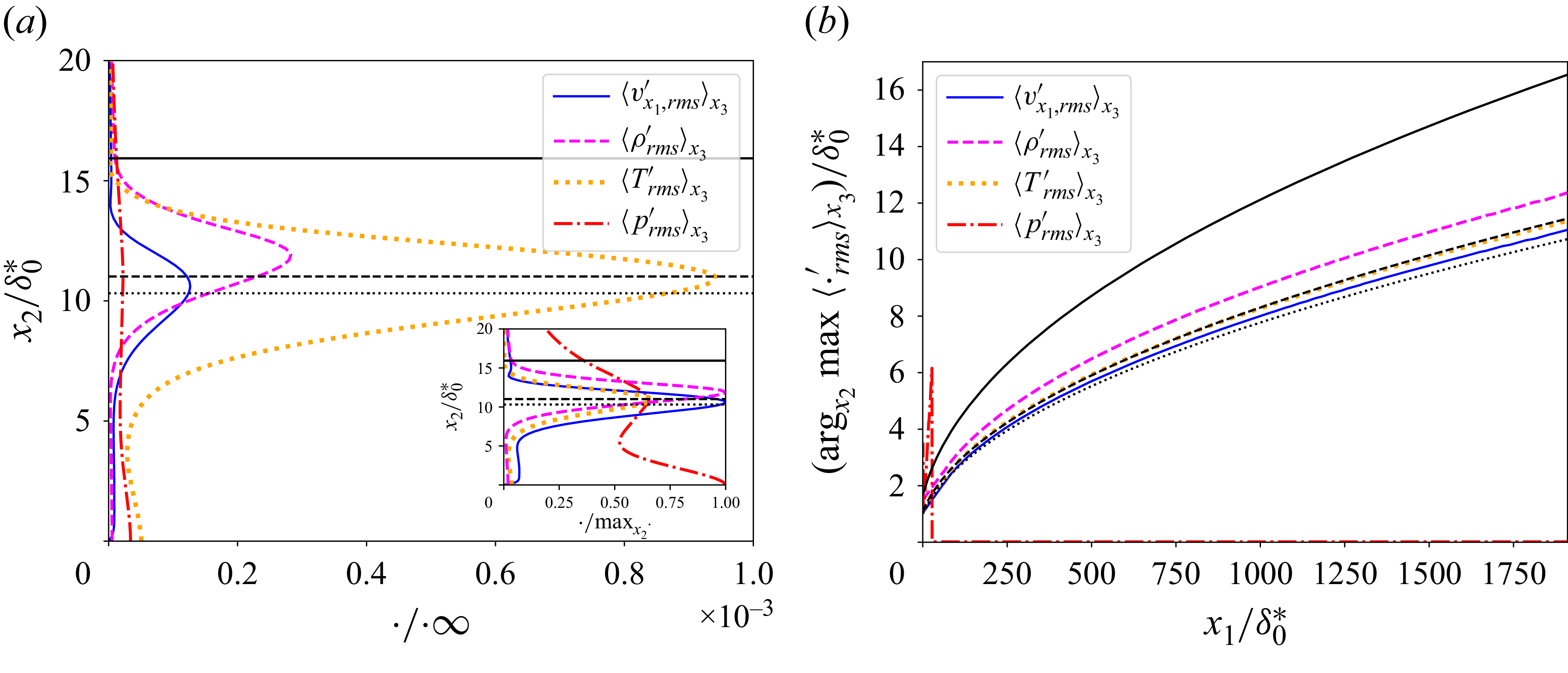
Spanwise-averaged PSD (each curve normalized by its own maximum) of fluctuating variables at
 $x_1=1775\delta _0^{*}$
, (a)
 $x_{2,\textit{GIP}}$
and (b)
 $x_2=0.015\delta _0^*$
(below
 $x_{2,\textit{GIP}}$
and very close to the wall) when the 3-D boundary layer is excited simultaneously by the
 $35$
uncorrelated white-noise signals
 $w^i$
.
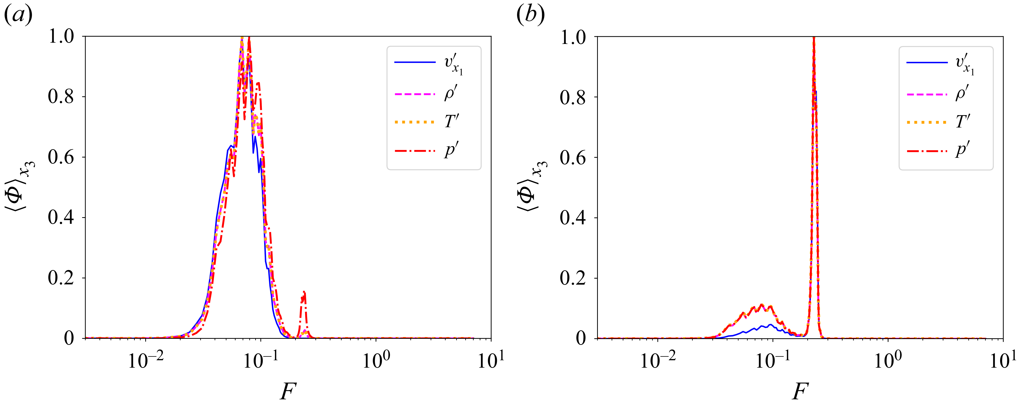
5.2. Selecting sensors
5.2.1. Performance sensors
As we wish to control both the first and the second modes, we select performance sensors capable of observing both phenomena. Therefore, sensors
 $\boldsymbol{z}_1,\boldsymbol{z}_2,\boldsymbol{z}_3$
which measure the wall-pressure, essentially observe the second Mack mode. Since the significance of oblique waves of the first mode may not be fully captured by wall-pressure measurements (see figure 7) (Chen et al. Reference Chen, Guo and Wen2023; Guo et al. Reference Guo, Hao and Wen2023), the additional row of performance sensors
 $\boldsymbol{z}_4$
is introduced to better capture the first instability mode by measuring the longitudinal velocity fluctuation at the generalized inflection point. These statements are confirmed by examining, in figure 8, the module of the transfer function
 $\hat {T}^k_{\phi (x_1) w}$
(obtained as the Fourier transforms of the impulse responses, see figure 5) from the noise sources to sensors
 $\phi (x_1)$
measuring (a)
 $v_{x_1}'$
at
 $x_{2,\textit{GIP}}$
and (b)
 $p'$
at the wall. Note that
 $|k|=17$
corresponds to
 $(|k|\beta /n)\delta _0^*\simeq 0.92$
. It is clear that the sensor
 $v_{x_1}'$
at
 $x_{2,\textit{GIP}}$
measures the first mode, since the dominant mode numbers correspond to oblique waves
 $k\neq 0$
. The wall-pressure sensors observe both the first (
 $k\neq 0$
) and second (
 $k=0$
) instability modes, with a predominant contribution from the latter. Figure 7 demonstrated that the frequency contents of the near-wall primitive variables are very similar (except for lower values of velocity fluctuations at low frequencies); therefore, it is expected that reducing the r.m.s. values of wall-pressure with destructive interference will also attenuate the near-wall velocity, density and temperature fluctuations. Conversely, reducing the r.m.s. values of longitudinal velocity perturbations should also attenuate pressure, density and temperature fluctuations at
 $x_{2,\textit{GIP}}$
as the frequency contents of primitive variables are similar. Indeed, the PSDs are also very similar, except near the peak at
 $F\sim 0.25$
which is more pronounced for pressure and less for velocity.
Modules of
 $\hat {T}^k_{\phi (x_1) w}$
for (a) velocity fluctuation performance sensors at the generalized inflection point and (b) wall-pressure fluctuation performance sensors.
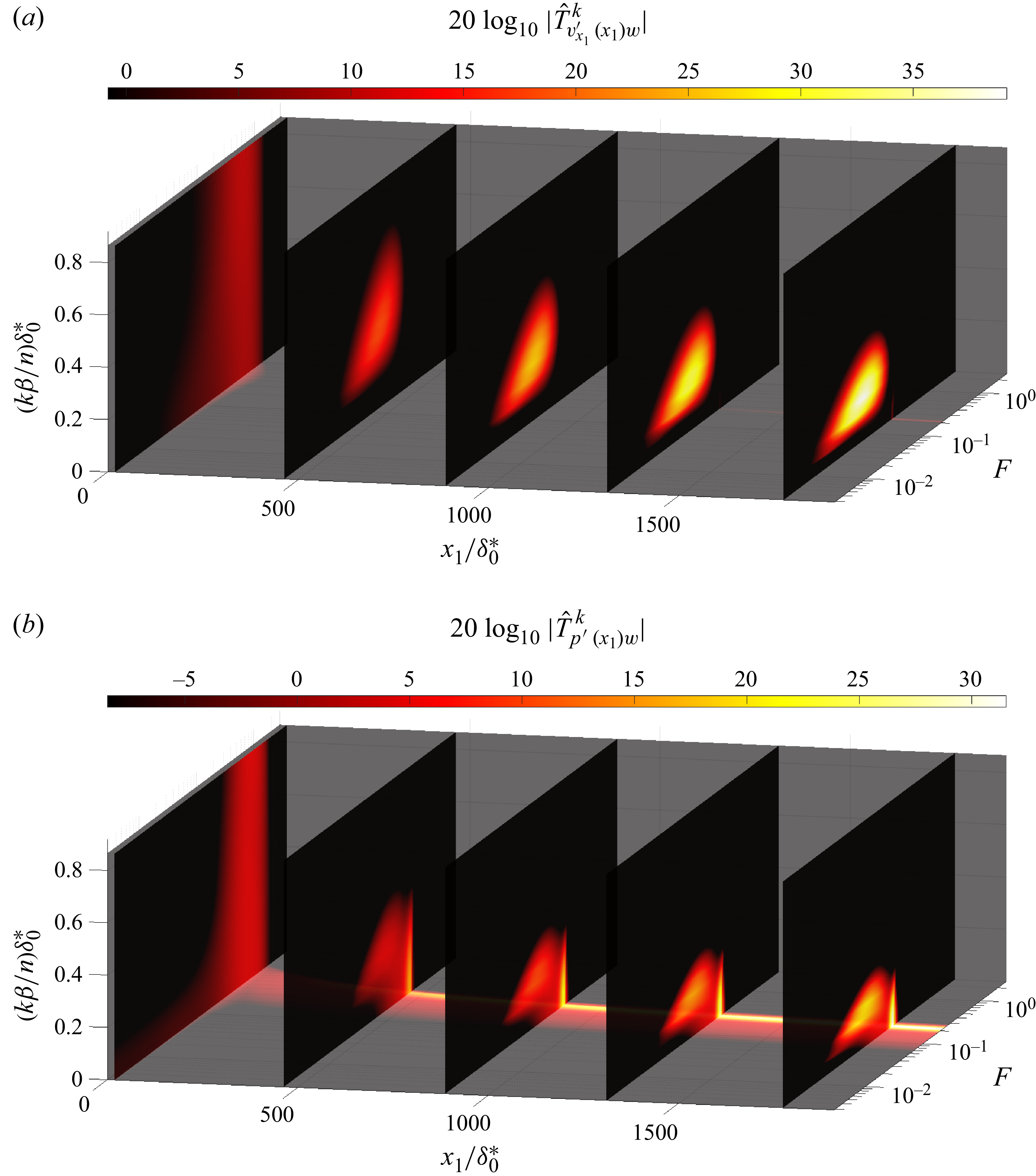
Since the control strategy works by destructive interference, we need to make sure the signature of actuation on performance sensors is not too dissimilar to that from noise sources. Therefore, we compare in figure 9 the module of the transfer functions from the noise sources to those from the actuators, for sensors
 $\boldsymbol{z}_3$
(wall-pressure) and
 $\boldsymbol{z}_4$
(velocity at
 $x_2=x_{2,\textit{GIP}}$
) at the end of the numerical domain. Figure 9(a,b) compares
 $\hat {T}^k_{z_4 u}$
with
 $\hat {T}^k_{z_4 w}$
: the main difference is that the signature of the second Mack mode is visible in the transfer from the actuators, while it is not in the transfer from the noise sources. Conversely in figure 9(c,d) comparing
 $\hat {T}^k_{z_3 u}$
with
 $\hat {T}^k_{z_3 w}$
, the signature of the first mode is not visible at the wall in the pressure signal from the actuators, while it is for the signal from the noise sources. These differences in the responses can be attributed to the fact that the disturbances generated by
 $\boldsymbol{u}$
do not take advantage of the full length of the instability domain contrary to the disturbances generated by
 $\boldsymbol{w}$
(see figure 3), leading to reduced amplification of the low frequency of the first mode and a relatively stronger contribution of the second mode. In addition, the spatial structure of the actuator forcing
 $b_u(x_3)$
favours low spanwise wavenumbers (in contrast to
 $b_w(x_3)$
, which corresponds to a Dirac distribution in the spanwise direction), further modifying the observed spectral response. Note that the differences in the responses from
 $\boldsymbol{w}$
and
 $\boldsymbol{u}$
have a detrimental effect for noise-cancellation by destructive interference. In future work, one may seek to optimize actuators in order to minimize these differences.
Comparison of the modules of transfer functions from
 $\hat {u}^k$
and
 $\hat {w}^k$
with the sensors at the end of the domain
 $\hat {z}_3^k$
(wall-pressure) and
 $\hat {z}_4^k$
(velocity at
 $x_{2,\textit{GIP}}$
): (a)
 $\hat {T}^k_{z_4 u}$
, (b)
 $\hat {T}^k_{z_4 w}$
, (c)
 $\hat {T}^k_{z_3 u}$
, (d)
 $\hat {T}^k_{z_3 w}$
. Note that
 $|k|=17$
corresponds to
 $(|k|\beta /n)\delta _0^*\simeq 0.92$
.
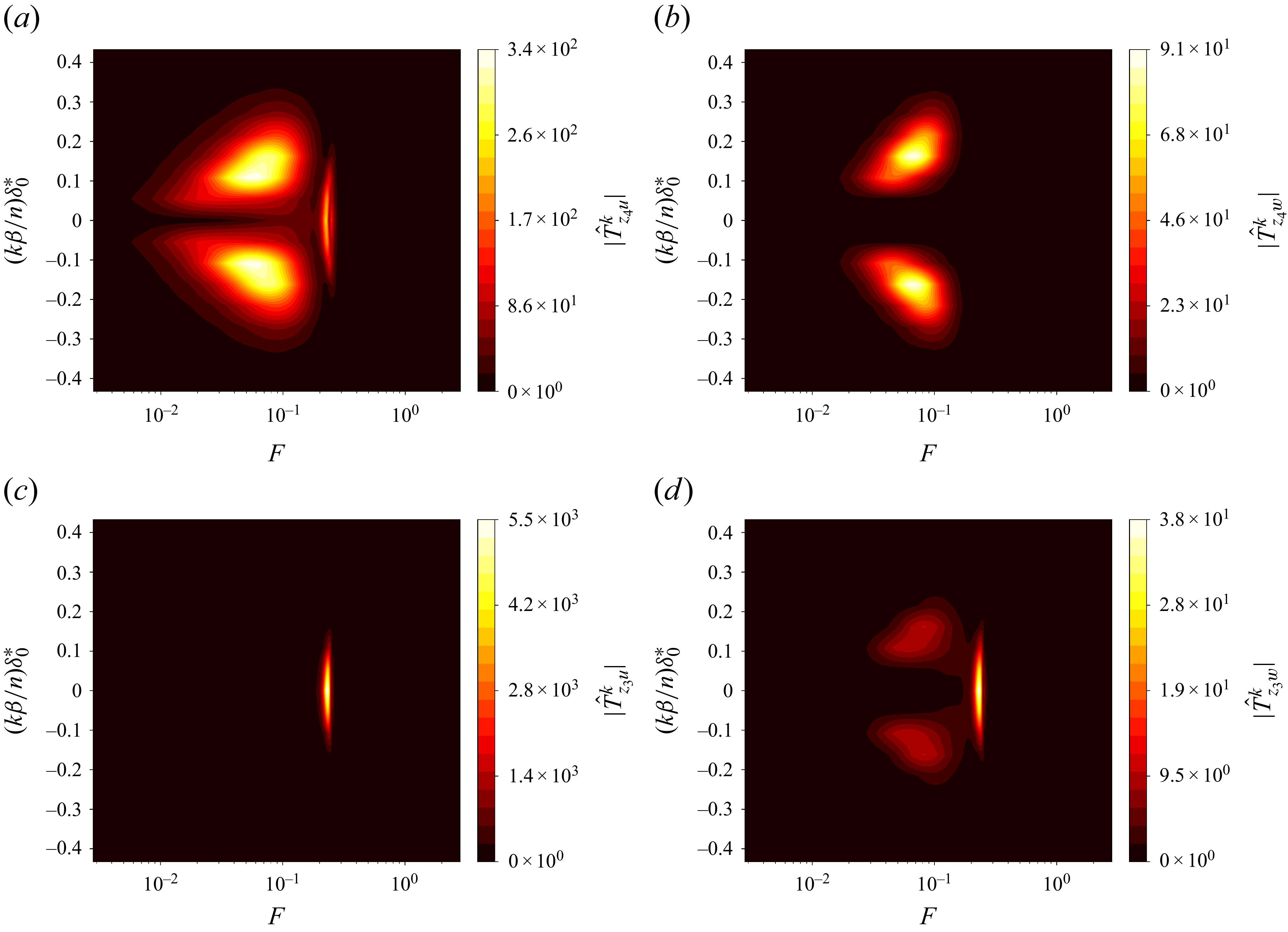
Figure 9. Long description
Panel A: A heat map showing the comparison of transfer function modules for wall-pressure sensors. The x-axis represents the variable F on a logarithmic scale ranging from 10^−2 to 10^0. The y-axis represents the variable (k beta/n) delta 0* ranging from −0.4 to 0.4. The color scale ranges from 0 to 340, with lighter colors indicating higher values. The heat map shows two distinct regions of high intensity. Panel B: A heat map showing the comparison of transfer function modules for wall-pressure sensors. The x-axis represents the variable F on a logarithmic scale ranging from 10^−2 to 10^0. The y-axis represents the variable (k beta/n) delta 0* ranging from −0.4 to 0.4. The color scale ranges from 0 to 91, with lighter colors indicating higher values. The heat map shows two distinct regions of high intensity. Panel C: A heat map showing the comparison of transfer function modules for velocity sensors. The x-axis represents the variable F on a logarithmic scale ranging from 10^−2 to 10^0. The y-axis represents the variable (k beta/n) delta 0* ranging from -0.4 to 0.4. The color scale ranges from 0 to 5500, with lighter colors indicating higher values. The heat map shows a single region of high intensity. Panel D: A heat map showing the comparison of transfer function modules for velocity sensors. The x-axis represents the variable F on a logarithmic scale ranging from 10^−2 to 10^0. The y-axis represents the variable (k beta/n) delta 0* ranging from −0.4 to 0.4. The color scale ranges from 0 to 38, with lighter colors indicating higher values. The heat map shows two distinct regions of high intensity.
For identification and control, we only consider a subset of Fourier modes
 $|k|\leqslant 5$
, capturing 90 % of the perturbation energy, as we shall see below. Figure 10 shows the evolution of
 $\|\hat {T}^{k}_{\phi (x_1)w}\|_{\infty }=\underset {F\in \mathbb{R}}{\sup }\ |\hat {T}^{k}_{\phi (x_1)w}(iF)|$
for
 $|k|\leqslant 8$
and
 $\phi (x_1)$
measuring either (a) velocity at
 $x_2=x_{2,\textit{GIP}}$
or (b) wall-pressure. After reaching a peak, the magnitude associated with a particular mode
 $k$
decreases for the highest modes. For the velocity sensors at
 $x_{2,\textit{GIP}}$
, spanwise modes that have a negligible energy contribution upstream of the domain are dominant downstream and the most energetic spanwise mode varies as a function of
 $x_1$
, contrary to the wall-pressure performance sensors, which are continuously dominated by
 $k=0$
. The number of modes
 $|k|\leqslant k_{90\,\%}$
necessary to capture
 $90\,\%$
of
 $\|T_{\phi (x_1)w}\|_2$
is depicted in figure 10(c,d). Given the selected position
 $\boldsymbol{u}$
of the actuators (see dashed vertical lines), we only consider modes
 $|k|\leqslant 5$
(see horizontal dotted line) for identification and synthesis because trying to control higher spanwise modes would have a negligible effect on the r.m.s. values of the performance sensors, which are located farther downstream. Note that even if
 $k_{90\,\%}=5$
, a greater number of sensors need to be chosen to avoid aliasing (see § 3.5). The choice
 $n=35$
is here more than sufficient. Of course, zero-padding in Fourier space is used to work with 35 actuators/sensors while controlling only 11 transverse modes.
Evolution of (a,b)
 $\|\hat {T}^{k}_{\phi (x_1)w}\|_{\infty }$
for
 $|k|\leqslant 8$
and (c,d) number of spanwise modes
 $k_{90\,\%}$
necessary to capture at least
 $90\,\%$
of
 $\|T_{\phi (x_1)w}\|_{2}$
for
 $\phi (x_1)$
measuring (a,c) velocity fluctuations at
 $x_{2,\textit{GIP}}$
and (b,d) wall-pressure fluctuations. The vertical dotted line represents the streamwise position
 $x_{1,\boldsymbol{u}}$
of the actuators. The spanwise modes
 $|k|\leq 5$
(below the horizontal dotted line in c and d) are those used in the identification and synthesis step.
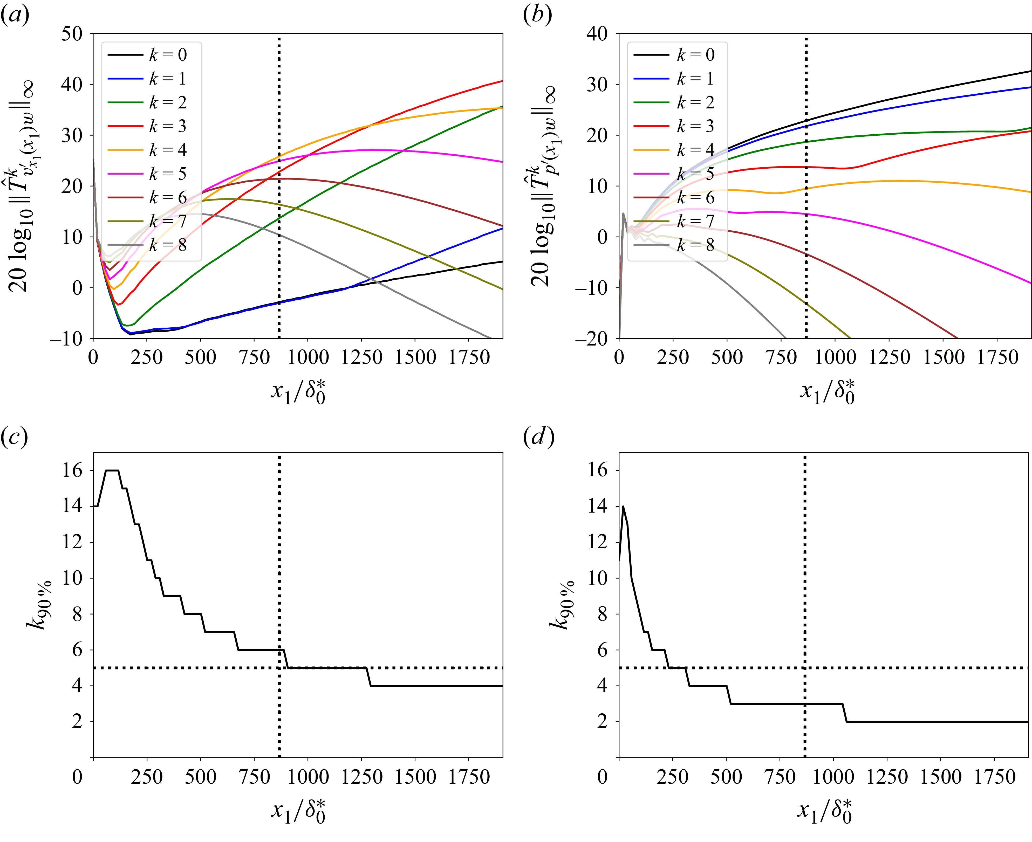
In this paragraph, we justify how the number of performance sensor rows was chosen, and how their longitudinal positions were selected. Of course, the set of performance sensors
 $\boldsymbol{z}_{\!j}$
must be representative of the dynamics to be controlled from the actuators to the end of the numerical domain. For the velocity sensors at
 $x_{2,\textit{GIP}}$
, as the frequencies
 $F$
contributing the most to the energy of a sensor close to the actuators are still non-negligible close to the end of the numerical domain used (see figures 3 and 8), minimizing the r.m.s. values of a single row
 $\boldsymbol{z}_4$
of velocity sensors downstream of the domain at
 $x_{1,\boldsymbol{z}_4}=1775\delta _0^*$
should also have a positive effect on the rows of sensors farther upstream. Choosing a row of sensors sufficiently far downstream also makes sense because the energy of the disturbances increases as they are convected, so the control must reduce consequently the energy downstream to avoid triggering nonlinearities which appear from a certain energy threshold: the farther downstream the disturbances are from the actuators, the more their energy must be reduced (Nibourel et al. Reference Nibourel, Leclercq, Demourant, Garnier and Sipp2023, Reference Nibourel, Leclercq, Demourant, Garnier and Sipp2024). For the wall-pressure sensors, the frequencies contributing to the energy of the second Mack mode near the actuators have a negligible impact downstream of the domain (see figures 3 and 8). To cover the entire amplified bandwidth of the second Mack mode from the actuators to the end of the domain, it is necessary to use several rows of sensors. Indeed, if all the dominant frequencies from the actuators to the end of the domain are not taken into account in the synthesis step, a harmful waterbed effect may occur: some frequencies can be amplified by the controller whereas they could be predominant in some abscissa of the plate (see Nibourel et al. Reference Nibourel, Leclercq, Demourant, Garnier and Sipp2023). In practice, three rows of wall-pressure sensors
 $\boldsymbol{z}_1,\boldsymbol{z}_2,\boldsymbol{z}_3$
are used for the synthesis, respectively, at
 $(x_{1,\boldsymbol{z}_1},\, x_{1,\boldsymbol{z}_2},\, x_{1,\boldsymbol{z}_3})=(1022.6,1312.2,1775.0)\delta _0^*$
. These positions are close to the ones used in the 2-D studies of Nibourel et al. (Reference Nibourel, Leclercq, Demourant, Garnier and Sipp2023, Reference Nibourel, Leclercq, Demourant, Garnier and Sipp2024) that allowed to obtain an efficient control of the second Mack mode in terms of disturbance amplitude reduction.
5.2.2. Estimation sensors
The estimation sensors
 $\boldsymbol{y}$
are wall-pressure fluctuation sensors. This choice is supported by the fact that both instability modes are observable by this type of sensor (see figure 8
b) and not only the oblique first mode as with the velocity sensors at
 $x_{2,\textit{GIP}}$
(see figure 8
a). In addition, unlike performance sensors
 $\boldsymbol{z}_{\!j}$
which are only used during synthesis and whose associated transfer functions could be modelled (e.g. by numerical calculations), estimation sensors
 $\boldsymbol{y}$
need to be physically implementable in realistic set-ups to compute the actuator signal
 $\boldsymbol{u}(t)$
from
 $\boldsymbol{K}$
. Wall-pressure sensors are indeed commonly used in hypersonic experimental set-ups (Lugrin et al. Reference Lugrin, Nicolas, Severac, Tobeli, Beneddine, Garnier, Esquieu and Bur2022). Only a feedback set-up where the estimation sensors are downstream of the actuators is employed in this 3-D study as a feedforward set-up where the estimation sensors are upstream of the actuators is unable to ensure performance robustness when free stream velocity variations are considered (Nibourel et al. Reference Nibourel, Leclercq, Demourant, Garnier and Sipp2023) even with multimodel or gain scheduling methods (Nibourel et al. Reference Nibourel, Leclercq, Demourant, Garnier and Sipp2024).
To control the high frequencies of the second Mack mode, the convection delay
 $\tau _{\boldsymbol{yu}}$
of the disturbances from
 $\boldsymbol{u}$
to
 $\boldsymbol{y}$
has to be small enough (Barbagallo et al. Reference Barbagallo, Dergham, Sipp, Schmid and Robinet2012; Juillet et al. Reference Juillet, Schmid and Huerre2013; Freire et al. Reference Freire, Cavalieri, Silvestre, Hanifi and Henningson2020). Considering that frequencies up to
 $F\sim 0.3$
must be controlled (see figure 3), the actuator/estimation sensor distance
 $V_{\infty }\tau _{\boldsymbol{yu}}$
must be less than
 $ V_{\infty }/f_c=2\pi \delta _0^*/F\sim 21\delta _0^*$
with
 $f_c$
the controllable bandwidth (Glad & Ljung Reference Glad and Ljung2000). For frequencies outside the bandwidth, the controller cannot attenuate their amplitude. Therefore, the greater the distance between the sensor and the actuator, the less effective the controller becomes in terms of disturbance amplitude reduction (Nibourel et al. Reference Nibourel, Leclercq, Demourant, Garnier and Sipp2023, Reference Nibourel, Leclercq, Demourant, Garnier and Sipp2024). The estimation sensors are placed at a distance of
 $20.4\delta _0^*$
from the streamwise position of the actuators, i.e.
 $x_{1,\boldsymbol{y}}=887.6\delta _0^*$
. By examining
 $|\hat {T}^k_{yu}|$
in figure 11, we see that there is energy up to
 $(|k|\beta /n)\delta _0^*=0.486$
(i.e.
 $|k|=9$
), so at least 18 sensors should be used to avoid aliasing (see § 3.5). Therefore, our choice
 $n=35$
is more than enough to avoid aliasing. Zero-padding in the Fourier domain is used since only modes up to
 $|k|=5$
will be controlled.
Module of
 $\hat {T}^k_{yu}$
.
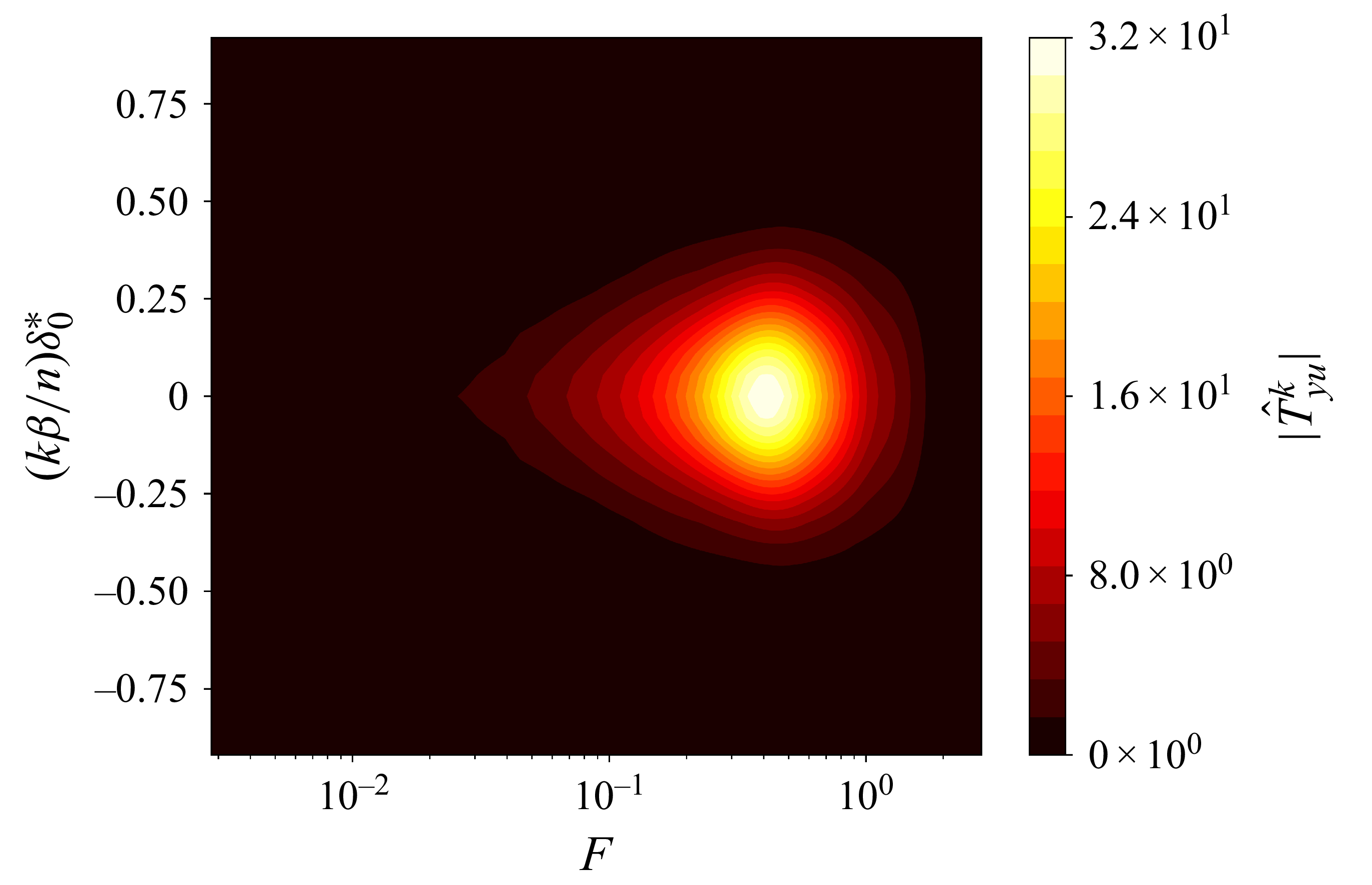
6. Identification and synthesis methods
6.1. System identification
Our synthesis methods require low-dimensional state-space realizations for all SISO transfer functions, for
 $k=0,\ldots, 5$
. These are obtained in a data-driven fashion. More specifically, we apply the eigensystem realization algorithm (Juang & Pappa Reference Juang and Pappa1985) on impulse response data as in Belson et al. (Reference Belson, Semeraro, Rowley and Henningson2013). Impulse responses are obtained from inverse Fourier transform of frequency responses as in Sasaki et al. (Reference Sasaki, Morra, Fabbiane, Cavalieri, Hanifi and Henningson2018, Reference Sasaki, Morra, Cavalieri, Hanifi and Henningson2020) and Morra et al. (Reference Morra, Sasaki, Hanifi, Cavalieri and Henningson2020).
The frequency response of the optimal filter
 $\hat {T}^k_{z_{\kern-1pt j} y_w}$
is obtained using estimates of the (cross-)PSDs from stochastic input/output signals, using Welch’s approach (Welch Reference Welch1967). A Savitzky–Golay of order two (Savitzky & Golay Reference Savitzky and Golay1964) and low/high pass filters (Butterworth Reference Butterworth1930) are also applied on
 $\hat {T}^k_{z_{\kern-1pt j} y_w}$
to smooth the frequency spectrum and to focus only on the dominant frequencies of the instability modes, respectively. The spectral factor
 $\hat {W}^k_{yw}$
is build from the magnitude data
 $\sqrt {\hat {\varPhi }^k_y}$
(estimated using the Welch method) and the MATLAB function fitmagfrd. For the frequency responses of
 $\hat {T}^{k}_{z_{\kern-1pt j}u}$
and
 $\hat {T}^{k}_{yu}$
, they are calculated by Fourier transform of the responses obtained from an impulse of one of the actuator in the absence of noise sources. As discussed in § 3.4, we remove a common deadtime
 $\tau _{\boldsymbol{z}_{\!j}\boldsymbol{y_w}}$
(convection delay from
 $\boldsymbol{y_w}$
to
 $\boldsymbol{z}_{\!j}$
) for the impulses from
 $\hat {y}_w^k$
and
 $\hat {u}^k$
to
 $\hat {z}_j^k$
prior to identification. This allows for a significant reduction in the order of the corresponding state-space realization.
The comparison of the ROMs (circles) and frequency/impulse data (solid lines) for
 $\hat {T}^k_{z_{\kern-1pt j} y_w}$
and
 $\hat {W}^k_{yw}$
used in the synthesis step is plotted in figure 12. To avoid overburdening the article, figures for
 $\hat {T}^{k}_{z_{\kern-1pt j}u}$
and
 $\hat {T}^{k}_{yu}$
are omitted. A good agreement is obtained and the ROMs capture most of the important dynamics. For a particular spanwise mode
 $k$
, the sum of the orders of each SISO ROM is
 $\sim 160$
. As we have to control modes up to
 $k=5$
, this would amount to work on a MIMO system potentially of order
 $\sim 960$
. Even though balanced truncation may be used to reduce the number of states, this illustrates the need to work on multiple decentralized SISO problems in the wavenumber space.
Comparison of the ROMs used in the synthesis (circles) and frequency/impulse data (solid lines) for (a,b)
 $\hat {W}^{k}_{yw}$
and (c,d)
 $\hat {T}^{k}_{z_3y_w}$
. For the ROMs of
 $\hat {T}^{k}_{z_3y_w}$
, the time axis of the impulse responses are shifted by
 $\tau _{\boldsymbol{z}_{\!j} \boldsymbol{y_w}}V_{\infty }/\delta _0^*\simeq 892$
which corresponds to the suppression of unnecessary dead times.
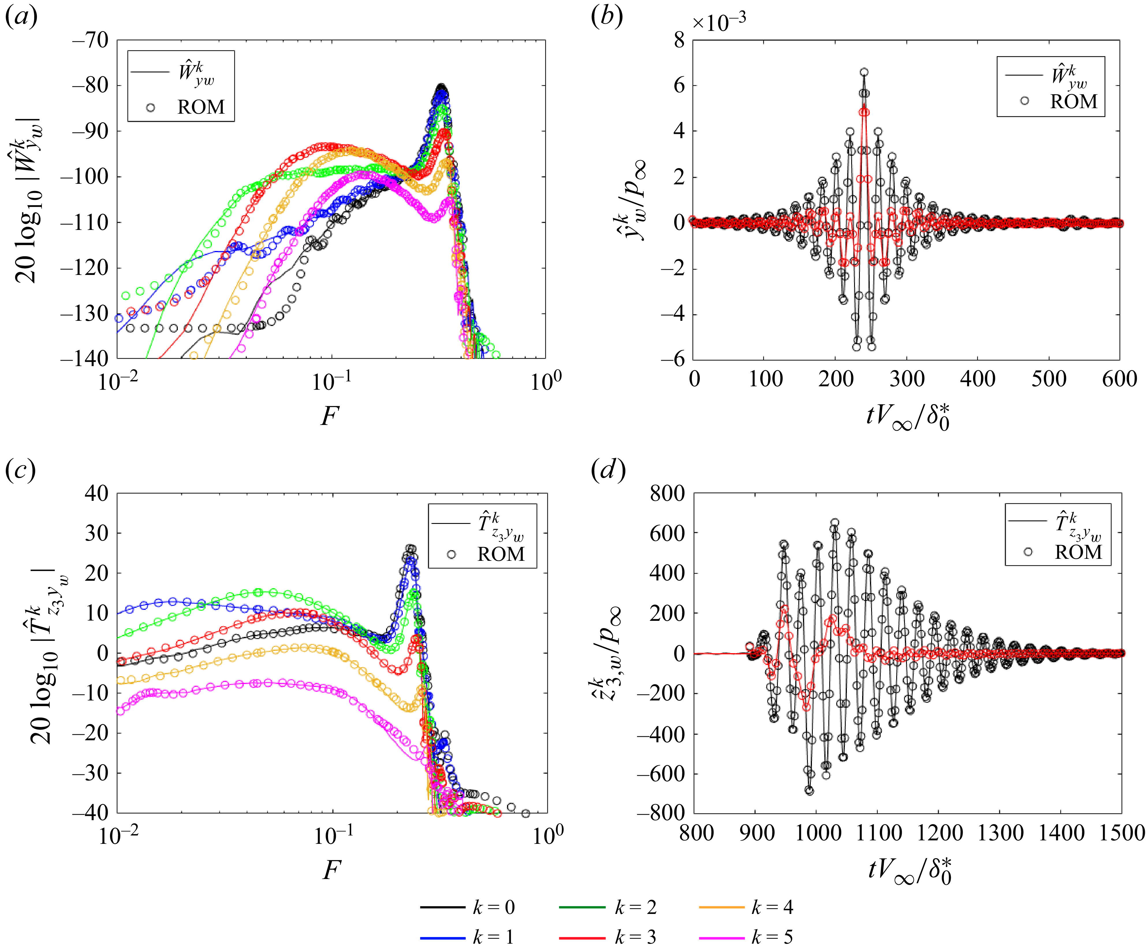
6.2. Constrained minimization problem
The structure of the six independent controllers
 $\hat {K}^{k}$
is imposed in the following way: each controller
 $\hat {K}^{k}$
is searched in state-space form with a strictly proper structure (inducing a roll-off of
 $-20$
dB per decade at high frequencies allowing to be robust to high-frequency noisy estimation sensors) and a tridiagonal state matrix; each controller
 $\hat {K}^{k}$
is stable and stabilizing with an order equal to
 $6$
. These specifications are similar to those imposed in the structured mixed
 $H_2/H_{\infty }$
syntheses of Nibourel et al. (Reference Nibourel, Leclercq, Demourant, Garnier and Sipp2023, Reference Nibourel, Leclercq, Demourant, Garnier and Sipp2024) for the 2-D control of the second Mack mode (so they were searching the ‘spanwise invariant’ controller
 $\hat {K}^{0}$
).
For each controller
 $\hat {K}^{k}$
with the structure imposed above, the MATLAB function systune (Apkarian et al. Reference Apkarian, Noll and Rondepierre2010, Reference Apkarian, Gahinet and Buhr2014) solves the following mixed
 $H_2$
/
 $H_{\infty }$
problem:
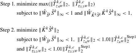 \begin{align} \begin{split} \text{Step 1.}\ &\text{minimize}\ \mathrm{max}(\|\hat {T}^{k,c}_{z_4w}\|_{2},\ \|\hat {T}^{k,c}_{\boldsymbol{z}_{1:3}w}\|_{2})\\ &\text{subject to}\ \|\hat {W}_{\hat {S}^{k}}\hat {S}^{k}\|_{\infty }\lt 1 \text{ and } \|\hat {W}_{\hat {K}^k\hat {S}^{k}}\hat {K}^k\hat {S}^{k}\|_{\infty }\lt 1,\\ \\ \text{Step 2.}\ &\text{minimize}\ \|\hat {K}^k\hat {S}^{k}\|_2\\ &\text{subject to}\ \|\hat {W}_{\hat {S}^{k}}\hat {S}^{k}\|_{\infty }\lt 1,\ \|\hat {T}^{k,c}_{z_4w}\|_{2}\lt 1.01\|\hat {T}^{k,c}_{z_4w}\|^{\text{Step1}}_{2}\\ &\text{and}\ \|\hat {T}^{k,c}_{\boldsymbol{z}_{1:3}w}\|_{2}\lt 1.01\|\hat {T}^{k,c}_{\boldsymbol{z}_{1:3}w}\|^{\text{Step1}}_{2}\ \end{split} \end{align}
with
 $\boldsymbol{z}_{1:3}=[z_1,z_2,z_3]^T$
. Hence, for a spanwise mode
 $k$
,
 $\hat {T}^{k,c}_{\boldsymbol{z}_{1:3}w}$
is a single-input–multiple-output (one input and three outputs) transfer function. This two step CMP is the transcription of the fluidic specifications established in § 4 and is explained in the following.
In step 1 of the CMP, the minimization of
 $\|\hat {T}^{k,c}_{z_4w}\|_{2}$
and
 $\|\hat {T}^{k,c}_{\boldsymbol{z}_{1:3}w}\|_{2}$
allows the reduction of r.m.s. values of both velocity sensors at the generalized inflection point and wall-pressure fluctuation sensors. To be able to compare these two types of sensors in the ‘
 $\text{minimize}\ \mathrm{max}$
’ formulation, their
 $H_2$
norms are normalized by the uncontrolled values (approximated by the six spanwise modes
 $k$
used in the synthesis)
 $\|\boldsymbol{T_{z_4w}}\|_{2}$
and
 $\|\boldsymbol{T_{z_{1:3}w}}\|_{2}$
, respectively. The results are therefore weighted by the importance that a spanwise mode has in the total energy. The
 $H_{\infty }$
constraint on
 $\hat {W}_{\hat {S}^{k}}\hat {S}^{k}$
maintains adequate stability margins (see § 4.2). The constant frequency template
 $\hat {W}_{\hat {S}^{k}}=0.5$
, implying
 $\|\hat {S}^{k}\|_{\infty }\lt 2$
, is used for all spanwise modes; this template provided substantial stability margins despite variations of
 $\pm 5\,\%$
of the free stream velocity in the 2-D studies of Nibourel et al. (Reference Nibourel, Leclercq, Demourant, Garnier and Sipp2023, Reference Nibourel, Leclercq, Demourant, Garnier and Sipp2024) (i.e. for the case
 $k=0$
). The frequency template
 $|1/\hat {W}_{\hat {K}^k\hat {S}^{k}}|=80\ \mathrm{dB}$
linked to the
 $H_{\infty }$
constraint on
 $\hat {W}_{\hat {K}^k\hat {S}^{k}}\hat {K}^k\hat {S}^{k}$
is just chosen as a very large constant so as not to constrain too much the actuator activity while rejecting ill-conditioned controller. In summary, this first algorithmic step returns controller
 $\hat {K}^{k}$
cancelling as much as possible velocity and pressure disturbances while ensuring important stability margins in the control bandwidth.
In step 2 of the CMP, a minimization of
 $\|\hat {K}^k\hat {S}^{k}\|_2$
is realized under the constraint of recovering similar results to step 1 in terms of pressure/velocity disturbance rejection. The same minimal stability margins than in step 1 are required through the frequency template
 $W_{\hat {S}^{k}}=0.5$
. The minimization of
 $\|\hat {K}^k\hat {S}^{k}\|_2$
serves a dual purpose: first, ensuring robust performance by desensitizing the controller to white noise corrupting the estimations sensors; second, by reducing the
 $H_2$
norm, one can also expect a reduction in the
 $H_\infty$
norm thereby contributing to robust stability objectives for additive uncertainties, particularly outside the bandwidth. This minimization complements the strictly proper structure of
 $\hat {K}^{k}$
which brings natural performance and stability robustness in high frequencies. This two-step resolution is explained by the fact that it is difficult to find weighting functions to compare
 $\|\hat {T}^{k,c}_{z_{\kern-1pt j}w}\|_{2}$
with
 $\|\hat {K}^k\hat {S}^{k}\|_2$
in a single minimization problem. The optimal results of the step 1 in terms of disturbance rejection (i.e.
 $\|\hat {T}^{k,c}_{z_4w}\|^{{Step1}}_{2}$
and
 $\|\hat {T}^{k,c}_{\boldsymbol{z}_{1:3}w}\|^{{Step1}}_{2}$
) are raised by a factor 1.01 in step 2 in order to obtain several controllers that respect these constraints before the algorithm starts the minimization procedure of
 $\|\hat {K}^k\hat {S}^{k}\|_2$
. In summary, the second algorithmic step is a trivial way to obtain controllers
 $\hat {K}^{k}$
reducing as much as possible amplitude of velocity/pressure disturbance, while ensuring desensitization of the loop to white noise corrupting the estimation sensors and robust stability in and outside the bandwidth. In other words, each controller
 $\hat {K}^k$
is designed to produce a control action in phase opposition to perturbations at its associated spanwise wavenumber
 $k$
(Sasaki et al. Reference Sasaki, Morra, Fabbiane, Cavalieri, Hanifi and Henningson2018, Reference Sasaki, Morra, Cavalieri, Hanifi and Henningson2020; Morra et al. Reference Morra, Sasaki, Hanifi, Cavalieri and Henningson2020). The
 $H_2/H_\infty$
structured feedback and decentralized design do not alter this principle but rather enforce deviations from ideal wave-cancellation to ensure feasibility, stability and robustness.
In steps 1 and 2, respectively, a dozen and a hundred random controller initializations are, respectively, performed to deal with the non-convex nature of the optimization problems. With the non-smooth algorithm employed and a parallel computation on 12 central processing unit cores (Intel(R) Xeon(R) CPU E5–2650 v3 @ 2.30 GHz), the six controllers
 $\hat {K}^{k}$
at the end of step 2 are obtained in approximately 2 hr (so around 20 min per controller
 $\hat {K}^{k}$
), which seems very reasonable for the control of a 3-D configuration.
7. Control performance and robustness
7.1. Linear regime
The results of the controlled system in a linear regime are analysed in this section, first on the nominal full-system (i.e. after implementation of the total 66th-order controller
 $\boldsymbol{K}$
in the CFD solver FastS), then in off-design operating conditions. The analysis of the results on the ROMs is provided in Appendix C.
7.1.1. On-design operating conditions
The frequency spectra of the spanwise modes for the performance sensors
 $\boldsymbol{z}_4$
and
 $\boldsymbol{z}_3$
after an impulse of the exogenous noise
 $w^0$
(at the centre spanwise position) are represented in figure 13. The control action reduces the amplitude of the dominant frequencies and spanwise modes of both the first and second instability modes. The amplitude of the dominant spanwise modes are reduced at each abscissa of the plate and control does not modify modes higher than
 $k=5$
(see figure 14) because we focused only on smaller modes in our synthesis (
 $\hat {K}^k=0$
for
 $k\geq 6$
). The quantity
 $\underset {x_1\gt x_{1,\boldsymbol{u}},\ k}{\max } \ln {\|\hat {T}^{k}_{\phi (x_1)w}\|_{\infty }}-\underset {x\gt x_{1,\boldsymbol{u}},\ k}{\max } \ln {\|\hat {T}^{k,c}_{\phi (x_1)w}\|_{\infty }}$
from the streamwise position of the actuators
 $x_{1,\boldsymbol{u}}$
until the end of the domain is, respectively, equal to
 $\sim 0.9$
and
 $\sim 0.85$
for the velocity and pressure performance sensors. From a local linear stability point of view, this quantity is akin to
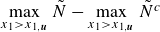 $\underset {x_1\gt x_{1,\boldsymbol{u}}}{\max }\ \tilde {N} - \underset {x_1\gt x_{1,\boldsymbol{u}}}{\max }\ \tilde {N}^c$
with
 $\tilde {N}$
and
 $\tilde {N}^c$
the
 $N$
-factor envelope of the uncontrolled and controlled cases, respectively. Performance improvements would mainly require modifying the actuator spatial support as well as the forced components to better match the instability structure induced by exogenous noise, thereby enhancing wave cancellation (Sasaki et al. Reference Sasaki, Morra, Cavalieri, Hanifi and Henningson2020), which is beyond the scope of the present study. By contrast, in the present configuration, increasing the number of actuators or reducing the streamwise distance between
 $\boldsymbol{u}$
and
 $\boldsymbol{y}$
is not expected to yield further gains, as these aspects are already near optimal (see § 3.5–5.2.2).
Comparison of the frequency spectra of the spanwise modes of the performance sensors (a,b)
 $\boldsymbol{z}_4$
and (c,d)
 $\boldsymbol{z}_3$
for the (a,c) uncontrolled and (b,d) controlled case.
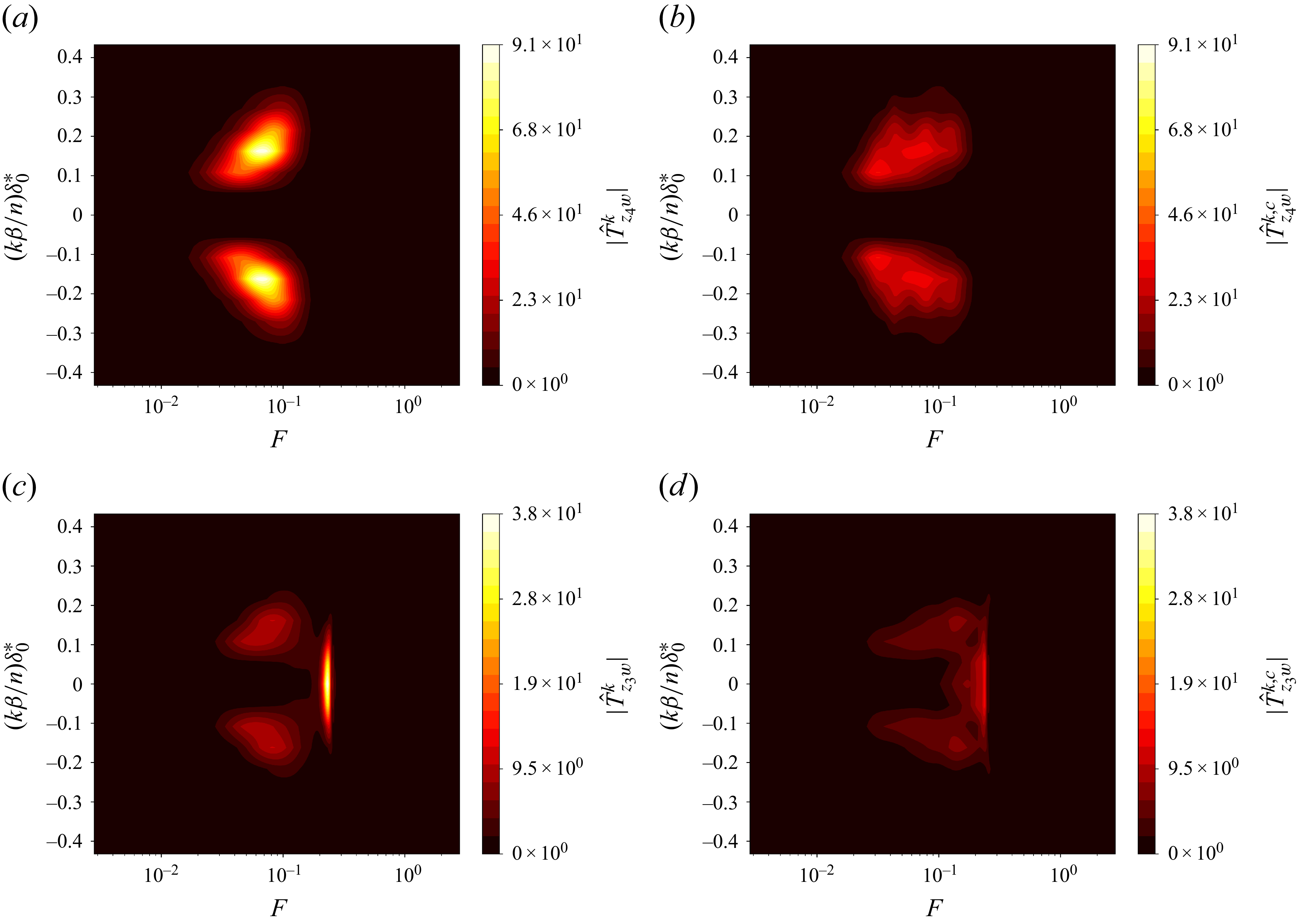
Figure 13. Long description
Panel A: A heat map showing the frequency spectra of spanwise modes for performance sensors in the uncontrolled case. The x-axis represents the frequency (F) on a logarithmic scale, and the y-axis represents the normalized wavenumber (kβ/nδ0*). The color scale ranges from black to yellow, indicating increasing values of the magnitude of the spanwise mode (|T̂zw|δ0*). Two distinct regions of high intensity are visible, one above and one below the center line. Panel B: A heat map showing the frequency spectra of spanwise modes for performance sensors in the controlled case. The axes and color scale are the same as in Panel A. The regions of high intensity are less pronounced compared to Panel A. Panel C: A heat map showing the frequency spectra of spanwise modes for another set of performance sensors in the uncontrolled case. The x-axis represents the frequency (F) on a logarithmic scale, and the y-axis represents the normalized wavenumber (kβ/nδ0*). The color scale ranges from black to yellow, indicating increasing values of the magnitude of the spanwise mode (|T̂zw|δ0*). A central region of high intensity is visible, with additional smaller regions above and below. Panel D: A heat map showing the frequency spectra of spanwise modes for another set of performance sensors in the controlled case. The axes and color scale are the same as in Panel C. The central region of high intensity is less pronounced compared to Panel C.
Evolution of
 $\|\hat {T}^{k}_{\phi (x_1)w}\|_{\infty }$
for
 $|k|\leqslant 8$
for
 $\phi (x_1)$
measuring (a) velocity fluctuation at
 $x_2=x_{2,\textit{GIP}}$
, (b) wall-pressure fluctuation. The vertical dotted line represents the streamwise position of the actuators. The norms
 $\|\hat {T}^{k}_{\phi (x_1)w}\|_{\infty }$
in (a) and (b) are normalized by
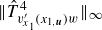 $\|\hat {T}^{4}_{v'_{x_{1}}(x_{1,\boldsymbol{u}})w}\|_{\infty }$
and
 $\|\hat {T}^{0}_{p'(x_{1,\boldsymbol{u}})w}\|_{\infty }$
, respectively, to express the potential gain in terms of the
 $N$
factor.
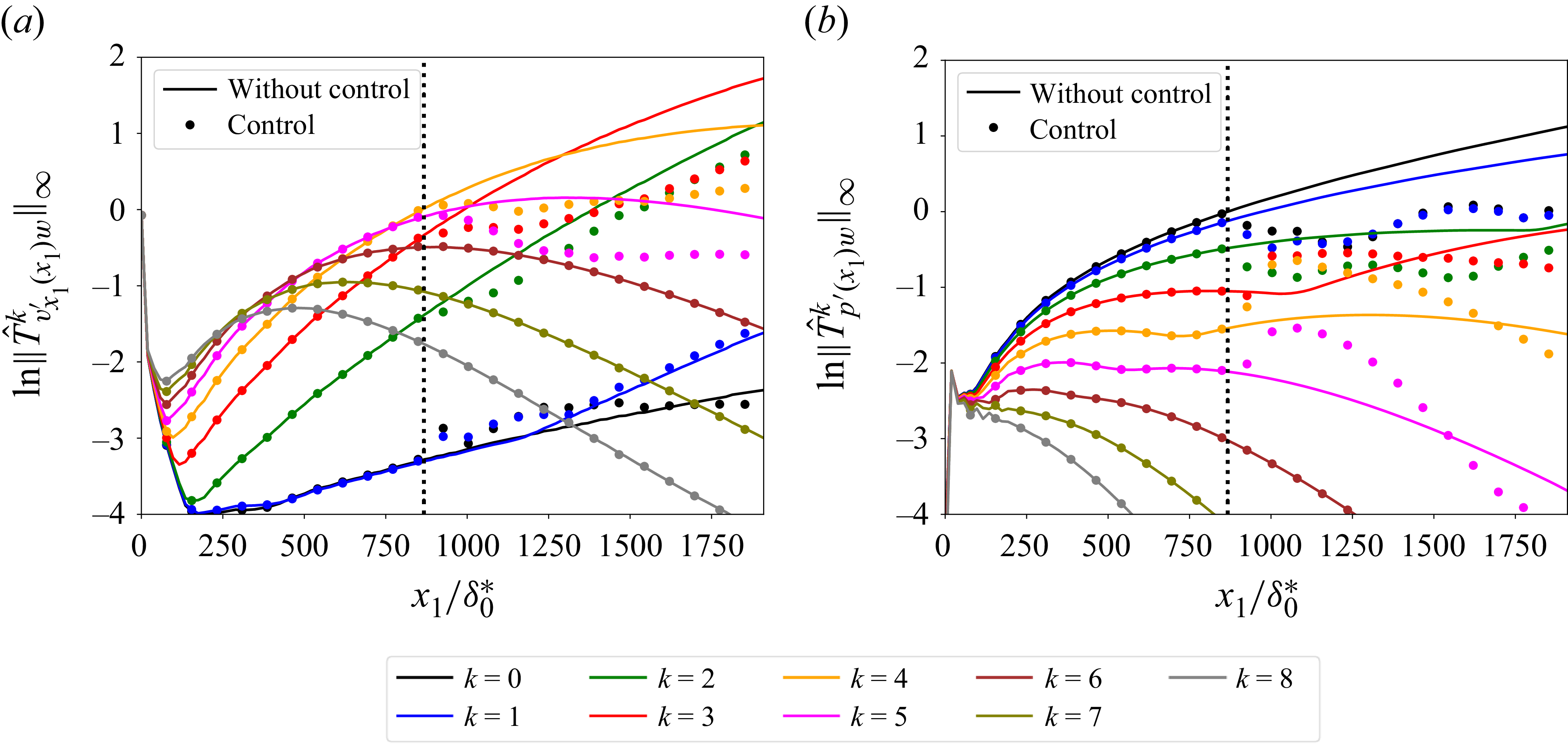
Beyond these results for the performance sensors, the performance is also evaluated by considering the r.m.s. values averaged in the spanwise direction when the 3-D boundary layer is excited simultaneously by the 35 uncorrelated white-noise signals
 $w^i$
.
For the r.m.s. velocity field (see figure 15 a), whose high values are located around the generalized inflection point due to the predominance of the first mode, the control reduces the amplitude of the perturbations. For the r.m.s. pressure field (see figure 15 b), the high values are located both close to the generalized inflection point and close to the wall due to the first and second mode, respectively. The reactive law controls simultaneously these two modes but an acoustic wave is generated at the location of the actuators. We will see in § 7.2 that this acoustic wave does not prevent delaying transition to turbulence so the resulting controller is deemed sufficiently satisfactory and performance robustness is addressed next.
Contours of (a)
 $v'_{x_1,\textit{rms}}$
and (b)
 $p'_{\textit{rms}}$
averaged in the spanwise direction for the (i) uncontrolled and (ii) controlled cases. The white solid and dashed lines, respectively, represent the boundary layer thickness
 $\delta$
and the generalized inflection point position
 $x_{2,\textit{GIP}}$
.
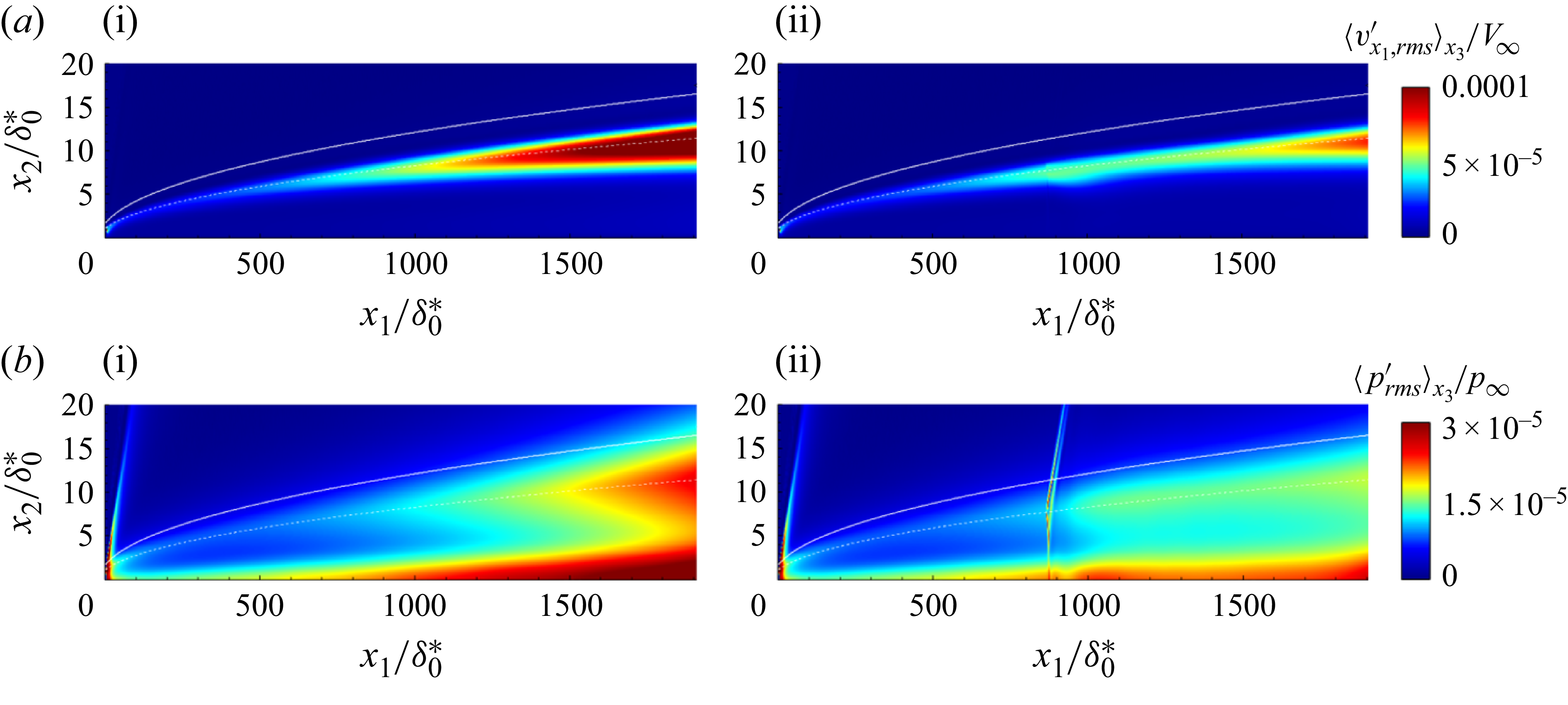
Figure 15. Long description
Panel A: Two heat maps showing the distribution of a variable related to flow dynamics. The x-axis is labeled x1/delta0* and ranges from 0 to 1750. The y-axis is labeled x2/delta0* and ranges from 0 to 20. The color scale on the right indicates the magnitude of the variable, with colors ranging from blue (low values) to red (high values). The white solid and dashed lines represent the boundary layer thickness and the generalized inflection point position, respectively. The left heat map shows the uncontrolled case, while the right heat map shows the controlled case. Panel B: Two heat maps showing the distribution of another variable related to flow dynamics. The x-axis is labeled x1/delta0* and ranges from 0 to 1750. The y-axis is labeled x2/delta0* and ranges from 0 to 20. The color scale on the right indicates the magnitude of the variable, with colors ranging from blue (low values) to red (high values). The white solid and dashed lines represent the boundary layer thickness and the generalized inflection point position, respectively. The left heat map shows the uncontrolled case, while the right heat map shows the controlled case.
7.1.2. Off-design operating conditions
In this section, performance robustness to off-design operating conditions is assessed by considering free stream velocity variations. The free stream velocity variations are the most problematic ones for noise-amplifier flows because they change the convective delays involving phase variations in the transfer functions, which may convert destructive interference into constructive ones (Nibourel et al. Reference Nibourel, Leclercq, Demourant, Garnier and Sipp2023). Moreover, Nibourel et al. (Reference Nibourel, Leclercq, Demourant, Garnier and Sipp2024) showed that with free stream velocity variations of only
 $5\,\%$
, the magnitudes of the dominant frequencies of the 2-D second Mack mode can vary by up to
 $80\,\%$
compared with the nominal case. Therefore, we will consider in this 3-D study free stream velocity variations of
 $2.5\,\%$
, which already represent a significant challenge for the system’s stability and performance.
In addition to modifying the aerodynamic delays, the variations of
 $V_{\infty }$
imply variations of
 $\pm 2.5\,\%$
of
 $M_{\infty }$
and
 $Re_{x_1}$
, since
 $\rho _{\infty }$
and
 $T_{\infty }$
are kept constant. New boundary layer profiles are used as inlet conditions and the previous controller
 $\boldsymbol{K}$
is directly implemented on the full 3-D system which is still excited by the 35 uncorrelated white noise sources
 $w^i$
with the same amplitudes as in the
 $M_{\infty }=4.5$
linearized DNS. It appears that the feedback control law is still stable, thanks to the important stability margins imposed in the synthesis (see § 6.2). The maxima along the wall-normal direction of
 $\lt v'_{x_1,\textit{rms}}\gt _{x_3}$
and
 $\lt p'_{\textit{rms}}\gt _{x_3}$
are plotted in figure 16. This figure shows that free stream velocity variations result in more significant amplitude changes for pressure instabilities compared with velocity instabilities, even in the absence of control. Concerning the controlled cases, the disturbance amplitudes are still reduced in off-design conditions thanks to the feedback set-up and its natural ability to maintain performance robustness over wide phase variations (Nibourel et al. Reference Nibourel, Leclercq, Demourant, Garnier and Sipp2024). Note that the higher the free stream velocity, the lower the intensity of the acoustic wave generated by the control. For this range of free stream variations, our simple feedback law is considered to be sufficiently robust in performance so that it is not necessary to further make robust some
 $\hat {K}^{k}$
(e.g. by multimodel synthesis or gain scheduling (Nibourel et al. Reference Nibourel, Leclercq, Demourant, Garnier and Sipp2024)).
Evolution of (a)
 $\max _{x_2} \lt v'_{x_1,\textit{rms}}\gt _{x_3}$
and (b)
 $\max _{x_2} \lt p'_{\textit{rms}}\gt _{x_3}$
after a variation of
 $V_{\infty }$
of
 $\pm 2.5\,\%$
. The nominal cases are in solid lines; the
 $+ 2.5\,\%$
and
 $- 2.5\,\%$
cases are, respectively, in dotted and dashed lines. The vertical magenta and black dotted lines represent, respectively, the streamwise positions of the actuators (with the sensors
 $\boldsymbol{y}$
nearby) and the performance sensors
 $\boldsymbol{z}_{\!j}$
used for synthesis.
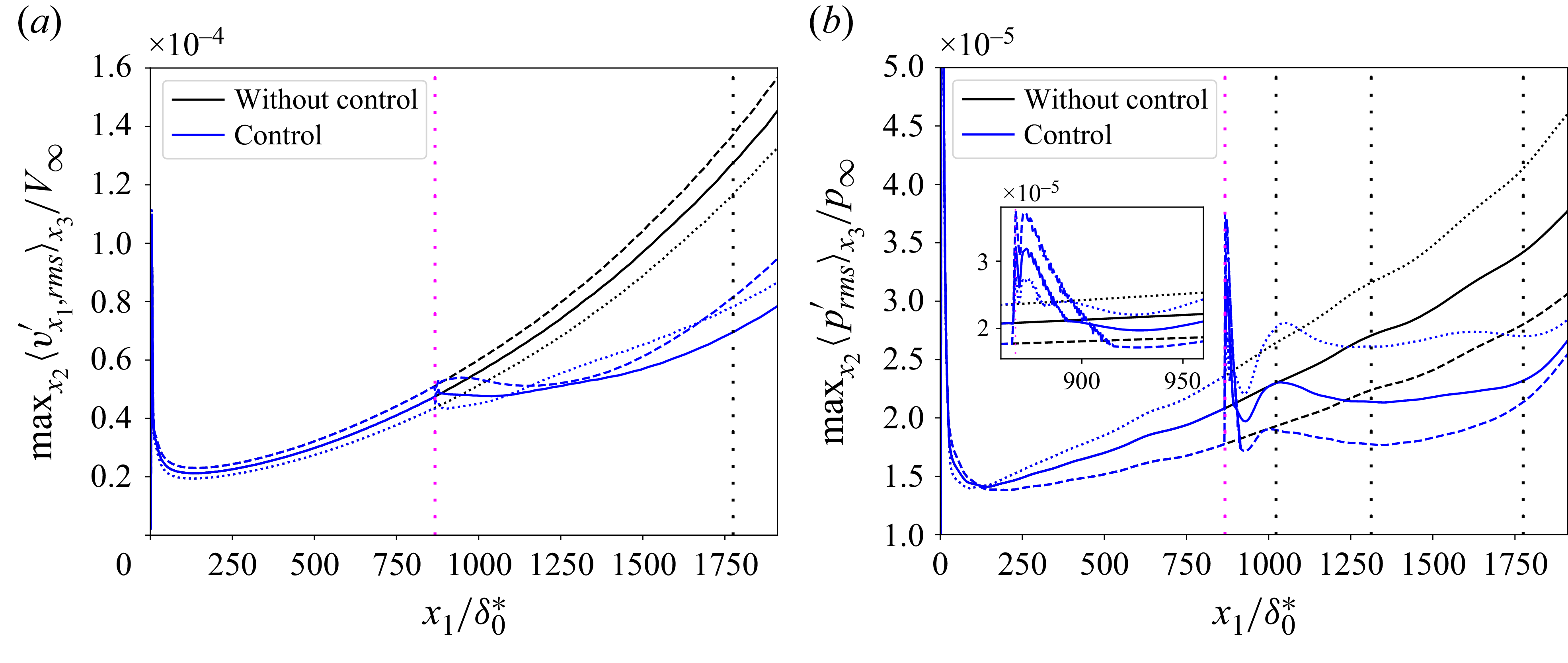
Performance robustness with respect to noise on the estimation sensors and with respect to the amplitude level of nonlinearities has also been evaluated but are reported in Appendix D and Appendix E, respectively. As a result, the control law still achieves high level of performance in terms of amplitude reduction despite a signal-to-noise ratio (SNR) of 0.53 (respectively, 2) in the case of high-frequency coloured noise (respectively, white noise) corrupting the estimation sensors
 $\boldsymbol{y}$
(see Appendix D) and despite exogenous noises leading to nonlinearities and velocity fluctuations up to
 $2\,\%$
of
 $V_\infty$
at the streamwise position of the estimation sensors (see Appendix E). Robustness to measurement noise is attributable to the CMPs (see § 6.2), whereas robustness to nonlinearities is just an observed outcome.
One could also assess the robustness of the controller to spanwise perturbations of the base flow but this is beyond the scope of our study. Note that the presence of a spanwise velocity component
 $v_{x_3,\infty }$
would not break the spanwise invariance of the present infinite-spanwise configuration. It would therefore still be possible to design a controller for this specific case by decomposing the MIMO system into independent SISO systems with the following specifications: firstly, the symmetry relation
 $\hat {T}^{-k}=\hat {T}^{k}$
would no longer hold, requiring independent synthesis of the positive and negative wavenumbers; secondly, the impulse responses between complex inputs and outputs would become also complex (contrary to Appendix B) leading to design each
 $\hat {K}$
as a
 $2\times 2$
MIMO controller (to treat the real and imaginary parts).
7.2. Transition to turbulence
Finally, the ability of the feedback law to delay transition to turbulence of a supersonic boundary layer is assessed. The length of the previous 3-D computational domain is doubled in the streamwise direction in order to obtain transition in the new domain while remaining weakly nonlinear from the streamwise position of the actuators to the end of the previous domain used in linearized DNS. By maintaining weak nonlinearity over this length, we mitigate both pressure and velocity disturbances up to at least
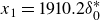 $x_1=1910.2 \delta _0^*$
; otherwise, the reduction of pressure disturbances risks dropping if the nonlinear effects are too significant from the actuator location (see Appendix E). For this new computational domain used for transition to turbulence, the boundary conditions and the wall-normal and spanwise lengths remain unchanged. The new streamwise length is
 $x_1 \in [0., 3820.4 \delta _0^*]$
; a sponge zone is added downstream of this domain, with the stretching of 30 cells in the streamwise direction and
 $L_{\textit{sponge}}=91.9\delta _0^*$
. A resolution of
 $6400\times 220\times 176$
is adopted (not including the sponge zone) and the spacings in the
 $x_1$
,
 $x_2$
,
 $x_3$
directions are the same as in the previous linearized DNS. This resolution ensures that
 $\varDelta x_1^+\lt 4$
,
 $\varDelta x_3^+\lt 3.5$
and
 $\varDelta x^+_{2,w\textit{all}}\lt 1$
in the entire domain (dimensionless grid size is defined as
 $\varDelta x^+_i=\sqrt {\tau _{w\textit{all}}\rho _{w\textit{all}}}\varDelta x_i/\mu _{w\textit{all}}$
with
 $\varDelta x_i$
corresponding to the grid spacing in direction
 $i$
of the Cartesian coordinate system).
The DNS of transition to turbulence is performed with exogenous noise sources with
 $\mathrm{Var}[w^i]=4$
. For comparison, the variance used in the linearized DNS was
 $\mathrm{Var}[w_{\textit{linear}}^i]=0.0016$
. With this noise intensity, the nonlinear effects are no longer negligible from
 $x_{1,{Nl}}=1284.6 \delta _0 ^*$
(see figure 17
a, first vertical black dotted line); this position is defined in this study when the relative difference between
 $\max _{x_2} \lt v'_{x_1,\textit{rms}}\gt _{x_3}$
of the linearized and nonlinear DNS is greater than
 $5\,\%$
. Hence, the nonlinear effects are low at the streamwise position of the actuators
 $x_{1,\boldsymbol{u}}$
. At
 $x_1=1910.2\delta _0^*$
(i.e. the end of the previous domain used for linearized DNS), the results differ by approximately
 $30\,\%$
. In the uncontrolled case, the start of transition to turbulence, defined by
 $\arg _{x_1} \min C_{\!f}$
(with
 $C_{\!f}= {\lt \tau _{w\textit{all}}\gt _{x_3,t}}/{0.5\rho _{\infty }V_{\infty }^2}$
), is at
 $x_{1,{Tr}}=2736.0\delta _0^*$
(see figure 17
b, second vertical black dotted line). The dotted curves that represent the skin friction of a laminar and a fully turbulent flat-plate boundary layer are also presented in this figure: the laminar curve comes from the DNS without exogenous noise sources whereas the turbulent one comes from the van Driest II correlation (Franko & Lele Reference Franko and Lele2013). In contrast to studies where the boundary layer is excited by a single primary mode, leading to a single common breakdown scenario, transition here occurs in the presence of multiple primary instability waves. One possible mechanism that could be considered is nonlinear interactions between the first and second modes, as described by Guo et al. (Reference Guo, Hao and Wen2023). Yet, this remains an open question in the present work because no detailed analysis of the transition scenario has been performed.
For exogenous noise sources with
 $\mathrm{Var}[w^i]=4$
, evolution of (a)
 $\max _{x_2} \lt v'_{x_1,\textit{rms}}\gt _{x_3}$
and (b)
 $C_{\!f}$
. The linear case (dashed line) in (a) is rescaled by multiplying its results by
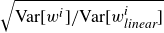 $\sqrt {\mathrm{Var}[w^i]/\mathrm{Var}[w_{\textit{linear}}^i]}$
for comparison. The magenta vertical line represents the streamwise position of the actuators. The first and second black vertical dotted lines represent the streamwise position from which the nonlinear effects are no longer negligible and the beginning of transition to turbulence, respectively. The black dashed curves in (b) represent the evolution of the skin friction coefficient for the fully laminar case (lower curve) and the turbulent case (upper curve).
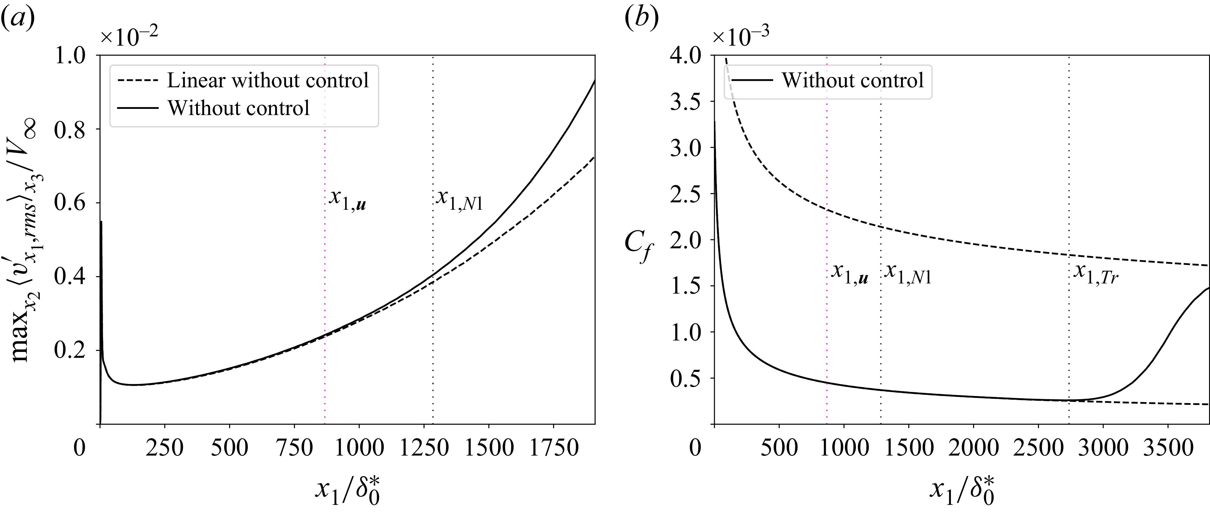
The feedback control drastically reduces the maximum amplitude of disturbances all along the new numerical domain (see figure 18). At the end of the domain for
 $x_1=3820.4\delta _0^*$
, the quantity
 $\max _{x_2}\ \lt ._{\textit{rms}}\gt _{x_3}$
is reduced by approximately
 $61\,\%$
and
 $27\,\%$
for
 $v_{x_1}'$
and
 $p'$
, respectively. Note that the intensity of the acoustic wave generated by the control near
 $x_{\boldsymbol{u}}$
is negligible compared with the values of the pressure fluctuations farther downstream of the domain and this acoustic wave does not prevent mitigation of the disturbance growth farther downstream (see figure 18
b). The profiles of
 $\lt v'_{x_1,\textit{rms}}\gt _{x_3}$
at different streamwise locations are plotted in figure 19. In the weakly nonlinear region (see figure 19
a), the controlled r.m.s. profile takes lower values than the uncontrolled r.m.s. profile on the whole wall-normal direction thanks to the control of both the first and the second instability modes. Even at a more downstream position where the nonlinear effects are much more important (see figure 19
b), the maxima of the profiles are still located near the generalized inflection point as long as the boundary layer remains laminar. At the beginning of transition to turbulence (see figure 19
c), the uncontrolled profile
 $\lt v'_{x_1,\textit{rms}}\gt _{x_3}$
starts to drop towards the wall while the maximum of the controlled profile is still near
 $x_{2,\textit{GIP}}$
. Finally, at
 $x_1=3300.5\delta _0^*$
(see figure 19
d), the maximum of the uncontrolled profile is located close to the wall while it remains farther above in the controlled profile, with much lower r.m.s. values. The fact that the collapse of the velocity profile is delayed in the controlled case is due to the delay of the breakdown stage thanks to the amplitude reduction of the modes up to
 $k=5$
and so weaker nonlinear interactions.
Evolution of
 $\max _{x_2} \lt ._{\textit{rms}}\gt _{x_3}$
for (a)
 $v_{x_1}'$
and (b)
 $p'$
for the transition case. For vertical lines, same caption as in figure 17.
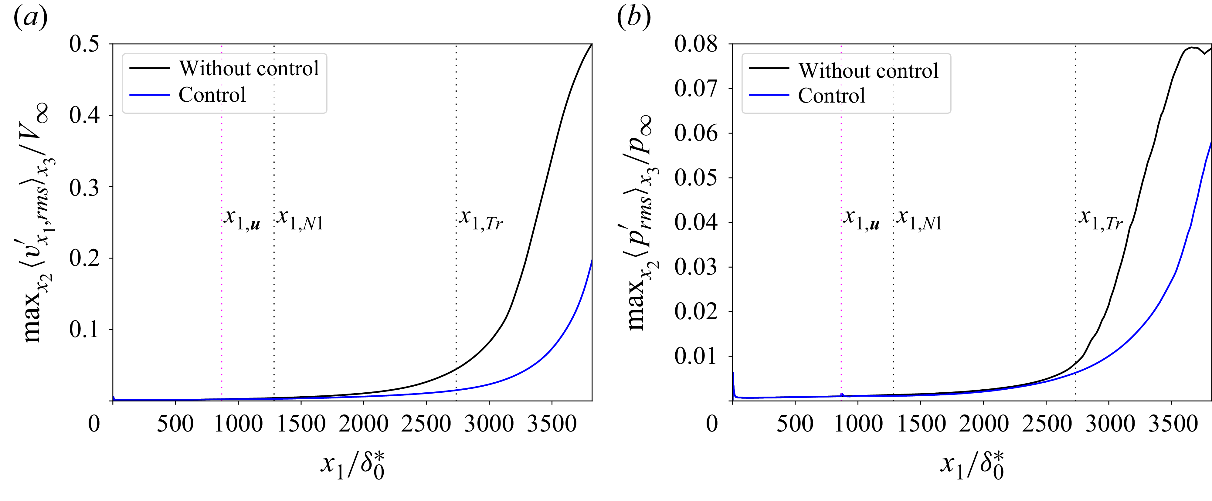
Profiles of
 $\lt v'_{x_1,\textit{rms}}\gt _{x_3}$
at (a)
 $x_1=x_{1,{Nl}}$
, (b)
 $x_1=1910.2\delta _0^*$
, (c)
 $x_1=x_{1,{Tr}}$
and (d)
 $x_1=3300.5\delta _0^*$
.
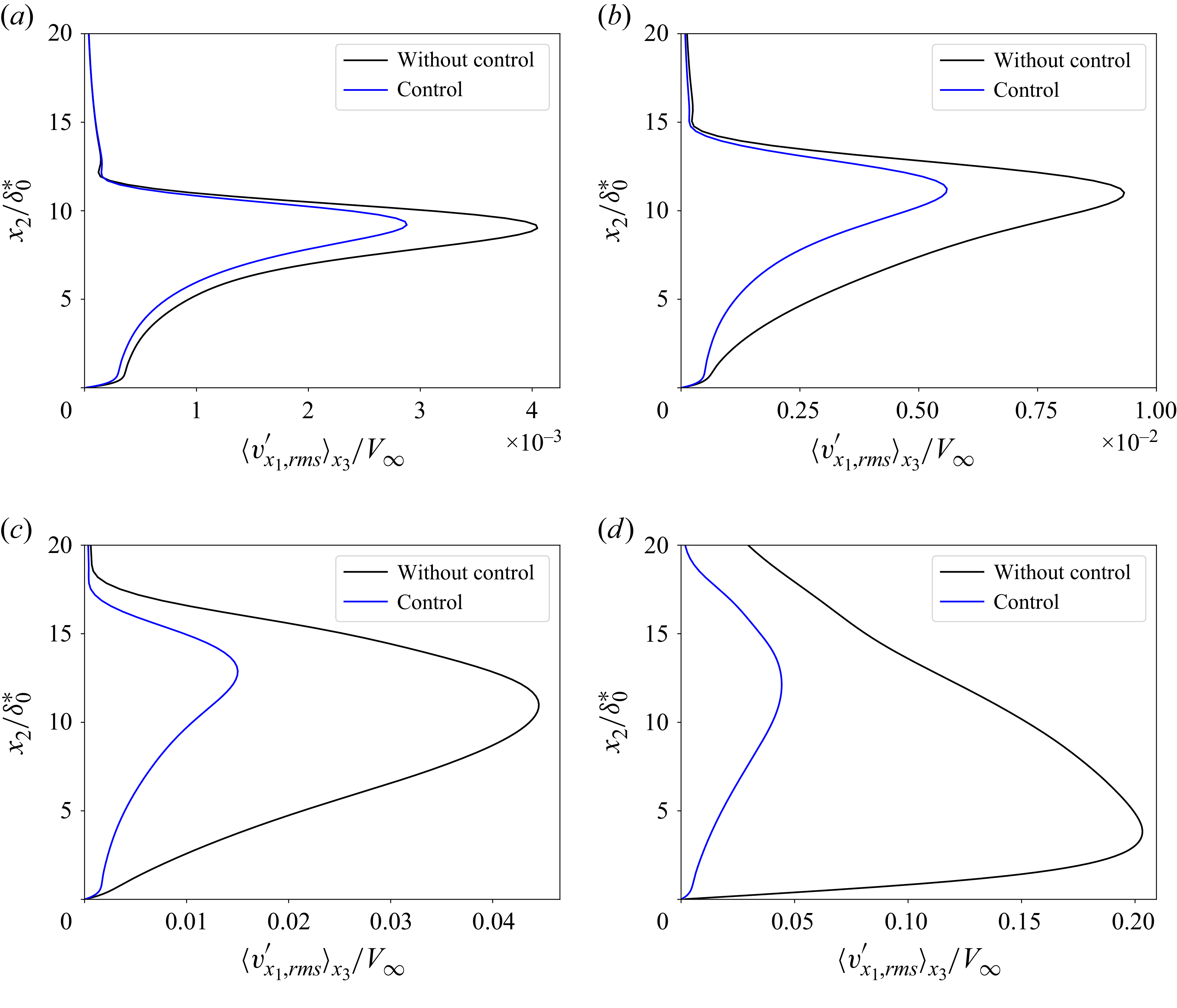
The instantaneous contours of streamwise velocity and numerical schlieren visualization are shown in figure 20. The uncontrolled flow presents chaotic structures while the controlled flow appears smoother. The emergence of turbulent structures is clearly delayed thanks to the control action. The laminar region is extended in the controlled case and transition to turbulence is delayed by
 $\varDelta x_{1,{Tr}}=564.4\delta _0 ^*$
(see figure 21); this distance represents
 $\sim 20 \,\%$
of the distance from the leading edge of the flat plate to abscissa of transition in the uncontrolled case (i.e.
 $19\delta _0^*+2736\delta _0^*$
). The delay in terms of
 $Re_{x_1}$
is
 $\varDelta Re_{x_1}=1.2\times 10^6$
.
Instantaneous contours of streamwise velocity (
 $x_1x_3$
-plane at
 $x_2=1.99\delta _0^*$
) and numerical schlieren visualization (
 $x_1x_2$
-plane at
 $x_3=0$
) between
 $2939.7\delta _0^*\lt x_1\lt 3820.4\delta _0^*$
for the (a) uncontrolled and (b) controlled cases.
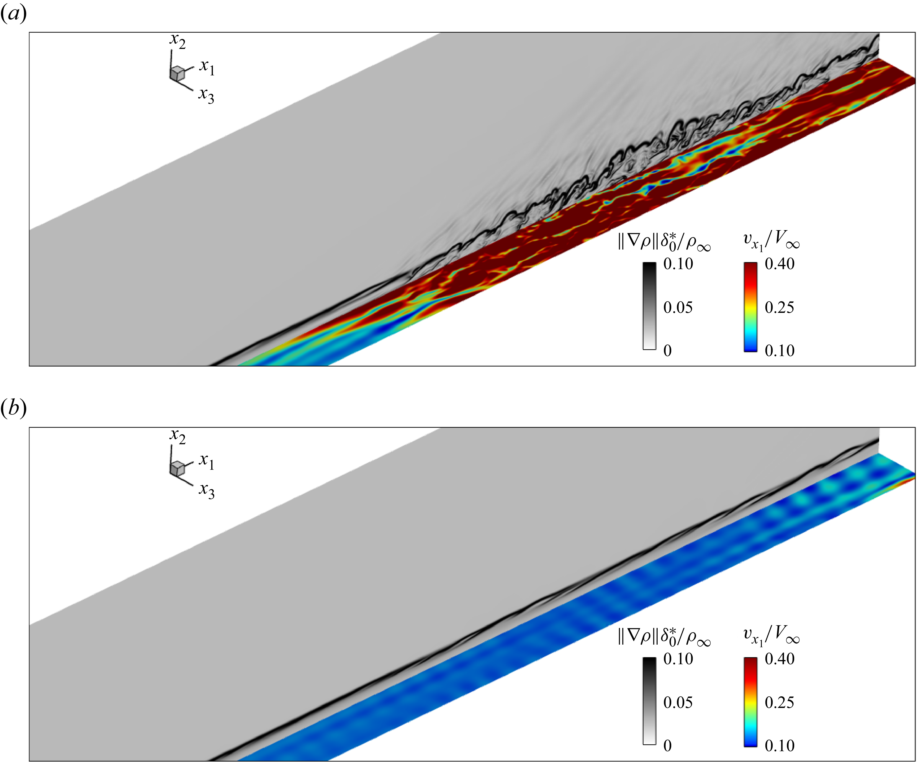
Figure 20. Long description
Panel A: A heat map representing the uncontrolled case. The x-axis and y-axis are labeled with coordinates x1 and x3, respectively. The color scale ranges from 0 to 0.10 for the magnitude of the gradient of density and from 0.10 to 0.40 for the normalized streamwise velocity. The heat map shows a gradient of colors from blue to red, indicating varying velocities and density gradients. The highest values are concentrated in the center, with a noticeable transition from blue to red. Panel B: A heat map representing the controlled case. The x-axis and y-axis are labeled with coordinates x1 and x3, respectively. The color scale ranges from 0 to 0.10 for the magnitude of the gradient of density and from 0.10 to 0.40 for the normalized streamwise velocity. The heat map shows a more uniform distribution of colors, predominantly blue, indicating lower velocities and density gradients compared to the uncontrolled case.
Evolution of the friction coefficient
 $C_{\!f}$
for the transition to turbulence case. The third black vertical dotted line represents the beginning of transition to turbulence for the controlled case. For other vertical lines, same caption as in figure 17.
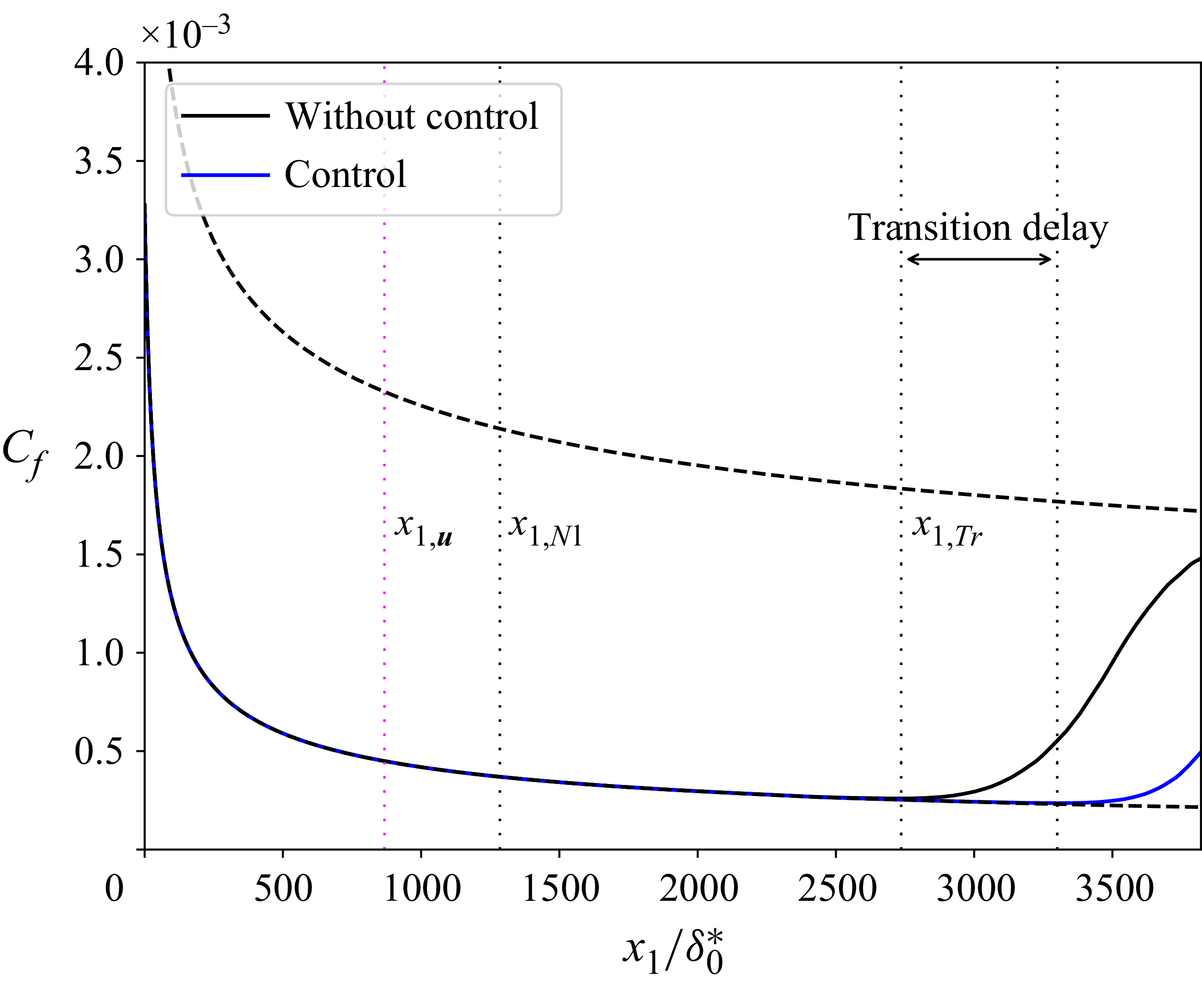
8. Conclusions
A robust reactive law has been developed to control both the linear growth of the first and second instability modes in a 3-D boundary layer over a flat plate at Mach 4.5 in order to delay transition to turbulence.
The estimation sensors are placed downstream of the actuators to have a feedback set-up and take advantage of its ability to be robust to free stream variations and model uncertainties. Performance sensors are wall-pressure fluctuation sensors and velocity fluctuation sensors at the generalized inflection point to have strong observability of the amplification mechanisms of the first and second modes. The MIMO centralized problem where all inputs are connected to all outputs is transformed to a SISO decentralized problem in the transverse wavenumber space where only one input is connected to one output. This greatly simplifies model identification and controller synthesis by solving multiple low-order independent problems instead of a single high-order problem and to spend control effort only on the spanwise modes associated with the most energetic structures. Indeed, the interconnection of the different modes is impossible in the linear growth stage.
The control law is built from linear tools where perturbations remain in the linear regime. The eigensystem realization algorithm is used for the identification procedure after shifting the time axis (removing dead times does not impact system norms) of some impulse responses to reduce the size of the ROMs. Then, structured mixed
 $H_2$
/
 $H_{\infty }$
synthesis is employed to impose the controller structure upfront and to obtain simultaneously in an optimal way nominal performance, stability robustness and performance robustness despite noisy estimation sensors.
The resulting controller, implemented in the CFD solver FastS, is first tested in linear regime. The control drastically reduces the amplitude of both the first and second instability modes. The performance robustness despite free stream velocity variations, which are the most problematic variations due to the modifications of the convective delays, is also ensured for variations of
 $\pm 2.5\,\%$
of
 $V_{\infty }$
thanks to the feedback set-up employed. The closed-loop is stable on these off-design conditions thanks to the large stability margins imposed in the synthesis. Still concerning performance robustness, the control law achieves amplitude reduction despite noisy estimation sensors (thanks to the resolved CMPs) or small nonlinearities near the actuators (though the synthesis remains purely linear, this robustness being an observed outcome).
The ability of the control law to delay transition to turbulence is finally assessed for a case where perturbations are weakly nonlinear at the streamwise position of the actuators. For this transition scenario, the control reduces the nonlinear interactions, resulting in delaying the turbulence breakdown of a distance representing
 $\sim 20 \,\%$
of the uncontrolled laminar zone from the upstream edge of the plate.
The experimental implementation of the proposed methodology mainly hinges on actuation and sensing capabilities. Effective control of the first and second modes would require actuators operating at very high frequencies, of the order of
 $O(10^5)$
Hz based on the present dimensional analysis (which likely points towards plasma-based actuation technologies, introducing additional technological and integration challenges). Moreover, sufficiently sensitive sensors are needed to detect very low-amplitude instability waves in order to keep the control action within a quasilinear regime (velocity fluctuations below approximately
 $1\,\%$
of the free stream value). These sensors must also provide a large bandwidth to capture the high-frequency content of instabilities. While the second Mack mode can be efficiently observed using wall-pressure sensors, the observability of the first mode using wall measurements alone remains challenging (Guo et al. Reference Guo, Hao and Wen2023), unless additional modelling is employed to reconstruct off-wall quantities such as velocity fluctuations at the generalized inflection point. Overcoming these controllability and observability limitations is a key step towards experimental validation of the present control strategy.
Acknowledgements
This work was partially funded by the French Agency for Innovation and Defence (AID). Their support was gratefully acknowledged.
Declaration of interests
The authors report no conflict of interest.
Appendix A. Grid and temporal convergence
The validation of the temporal and spatial schemes used in the 3-D DNS is performed by grid and temporal convergence analyses. The transfer function from the exogenous noise at the centre spanwise position
 $w^0$
to a wall-pressure fluctuation sensor (figure 22
a) and a velocity fluctuation sensor at the generalized inflection point (figure 22
b), both located at
 $x_3=0$
and
 $x_1=868.5\delta _0^*$
(just downstream of the actuators) is plotted as a function of the mesh resolution. The baseline mesh (BM) used throughout this article has a resolution of
 $3200\times 220\times 176$
cells (black solid lines); the streamwise and spanwise resolutions are refined independently. A refinement in the streamwise direction (blue dashed lines) slightly modifies the gain of the high frequencies of the second Mack mode while the low frequencies of the first instability mode are not impacted. A refinement in the spanwise direction (red dotted lines) does not modify the results obtained with the BM. The temporal convergence of the linearized 3-D DNS is validated by comparing the previous transfer functions as a function of the CFL number (see figure 22
c,d); the same results are obtained for the baseline CFL number lower than 0.7 (black solid lines) and for a CFL number lower than 0.35 (red dotted lines) in the whole 3-D domain. According to these results, the temporal and spatial schemes used throughout the article are deemed sufficient to compute the dynamics of the first and second instability modes and for the performance/robustness assessment of the control law. Note that the BM provides around 25 points per streamwise and spanwise wavelength for
 $F\simeq 0.4$
and
 $k=8$
, which correspond to the frequency and spanwise wavenumber with low energy content relative to the amplitude peaks (see figure 9). Consequently, the energetically dominant structures are resolved with an even finer spatial resolution.
(a,b) Grid and (c,d) temporal convergences of the gain of transfer function from the exogenous noise at the centre spanwise position
 $w^0$
to (a,c) wall-pressure performance sensor and (b,d) velocity performance sensor at the generalized inflection point, both located at
 $x_3=0$
and
 $x_1=868.5\delta _0^*$
.
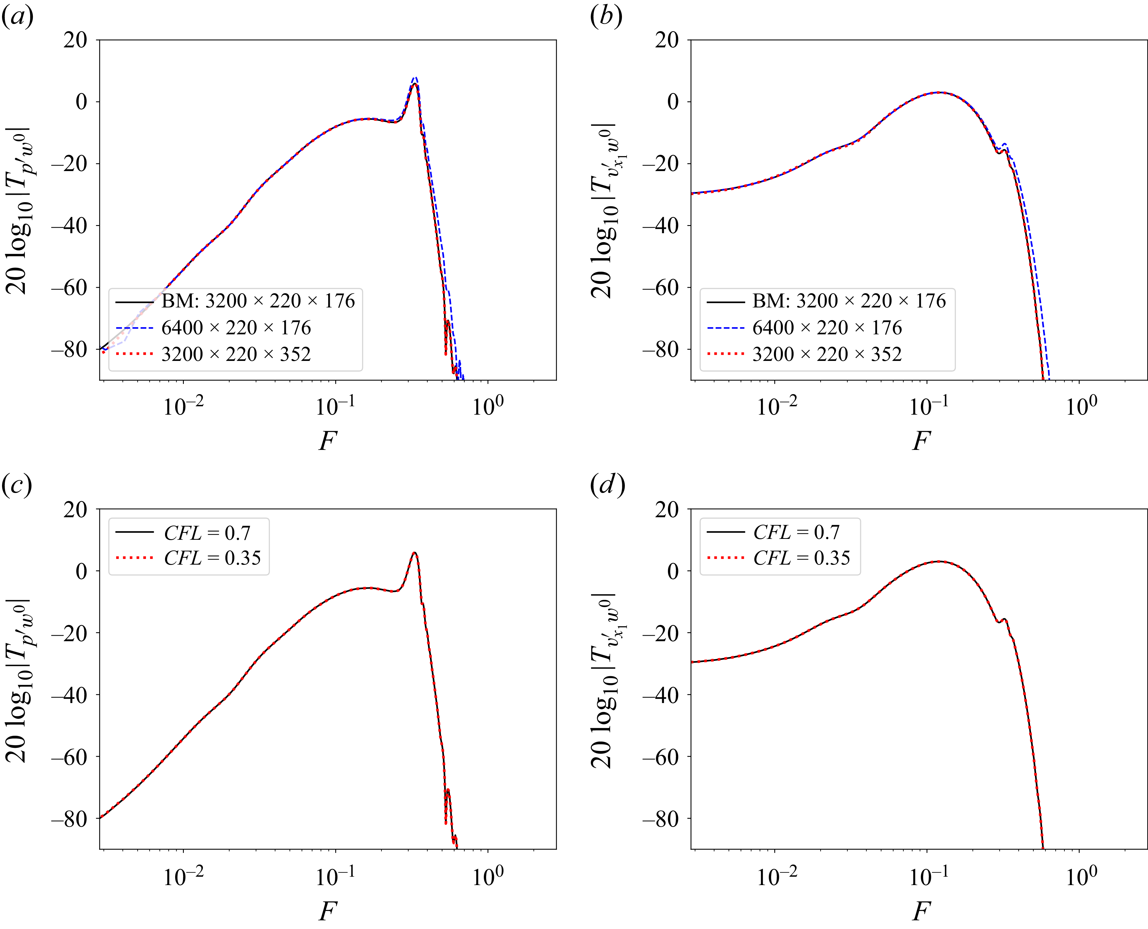
Figure 22. Long description
The image contains four line graphs labeled (a), (b), (c), and (d). Each graph shows the convergence of the gain of the transfer function from the exogenous noise at the center spanwise position. Panel A: A line graph showing the grid convergence of the transfer function gain for the wall-pressure performance sensor. The x-axis represents the frequency (F) on a logarithmic scale, and the y-axis represents the gain in decibels (20 log10|Tpp/w00|). The graph includes three lines representing different grid resolutions: 3200 x 220 x 176, 6400 x 220 x 176, and 3200 x 220 x 352. Panel B: A line graph showing the grid convergence of the transfer function gain for the velocity performance sensor. The x-axis represents the frequency (F) on a logarithmic scale, and the y-axis represents the gain in decibels (20 log10|Tvx1,w00|). The graph includes three lines representing different grid resolutions: 3200 x 220 x 176, 6400 x 220 x 176, and 3200 x 220 x 352. Panel C: A line graph showing the temporal convergence of the transfer function gain for the wall-pressure performance sensor. The x-axis represents the frequency (F) on a logarithmic scale, and the y-axis represents the gain in decibels (20 log10|Tpp/w00|). The graph includes two lines representing different Courant-Friedrichs-Lewy (CFL) numbers: 0.7 and 0.35. Panel D: A line graph showing the temporal convergence of the transfer function gain for the velocity performance sensor. The x-axis represents the frequency (F) on a logarithmic scale, and the y-axis represents the gain in decibels (20 log10|Tvx1,w00|). The graph includes two lines representing different CFL numbers: 0.7 and 0.35.
Appendix B. Real impulse responses between complex inputs and outputs
Decompose the state
 $\boldsymbol{q}$
into a vector field
 $\boldsymbol{\eta }=[\rho, \rho v_{x_1}, \rho v_{x_2}, \rho E]^T$
and the field of transverse momentum
 $\zeta =\rho v_{x_3}$
, such that, up to a reordering of variables,
 $\boldsymbol{q}=[\boldsymbol{\eta }^T,\zeta ]^T$
. Next, decompose the state variables
 $\boldsymbol{\eta }$
and
 $\zeta$
and the corresponding volume forcings
 $\boldsymbol{f}_{\boldsymbol{\eta }}$
and
 $\boldsymbol{f}_{\zeta }$
into Fourier series in the transverse direction
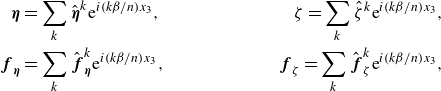 \begin{align} \boldsymbol{\eta }&=\sum _k \hat {\boldsymbol{\eta }}^k \mathrm{e}^{{i}(k\beta /n) x_3},\quad &\zeta =\sum _k \hat {\zeta }^k \mathrm{e}^{{i}(k\beta /n) x_3},\nonumber \\ \boldsymbol{f}_{\boldsymbol{\eta }}&=\sum _k \hat {\boldsymbol{f}}_{\boldsymbol{\eta }}^k\mathrm{e}^{{i}(k\beta /n) x_3},\quad &\boldsymbol{f}_{\zeta }=\sum _k \hat {\boldsymbol{f}}_{\zeta }^k \mathrm{e}^{{i}(k\beta /n) x_3}, \end{align}
where
 $\beta =2\pi /\varDelta _{x_3}$
is the fundamental transverse wavenumber based on the transverse distance between sensors/actuators. Given the transverse invariance of the base flow, and the absence of transverse base flow, it may be shown that the governing equations for each mode
 $k$
read
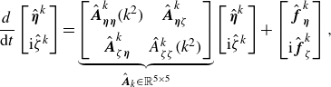 \begin{align} \dfrac {{d}}{\mathrm{d}t}\begin{bmatrix}\hat {\boldsymbol{\eta }}^k\\[5pt]\mathrm{i}\hat {\zeta }^k \end{bmatrix}=\underbrace {\begin{bmatrix} \hat {\boldsymbol{A}}^k_{\boldsymbol{\eta }\boldsymbol{\eta }}(k^2) & \hat {\boldsymbol{A}}^k_{\boldsymbol{\eta }\zeta }\\[5pt] \hat {\boldsymbol{A}}^k_{\zeta \boldsymbol{\eta }} & \hat {A}^k_{\zeta \zeta }(k^2) \end{bmatrix}}_{\hat {\boldsymbol{A}}_k\in \mathbb{R}^{5\times 5}}\begin{bmatrix}\hat {\boldsymbol{\eta }}^k\\[5pt]\mathrm{i}\hat {\zeta }^k \end{bmatrix}+\begin{bmatrix} \hat {\boldsymbol{f}}_{\boldsymbol{\eta }}^k \\[5pt] \mathrm{i}\hat {\boldsymbol{f}}_{\zeta }^k \end{bmatrix}, \end{align}
where all matrices are real, despite the inputs and outputs being complex. The detail of the equations is provided in Appendix A of Robinet (Reference Robinet2007) for a state vector in primitive variables, but the above structure is identical in conservative variables. Given our choices of sources and sensors, all transfer functions are derived from the transfer function from
 $\boldsymbol{f}_{\boldsymbol{\eta }}$
to
 $\boldsymbol{\eta }$
,
 \begin{align} \hat {\boldsymbol{T}}^k_{\boldsymbol{\eta }\boldsymbol{\eta }}(s)=\big(s\boldsymbol{I}-\hat {\boldsymbol{A}}^k_{\boldsymbol{\eta }\boldsymbol{\eta }}(k^2) \big)^{-1}. \end{align}
More specifically, for both the noise and the actuator sources, the corresponding forcing field reads
 $\boldsymbol{f}_{\boldsymbol{\eta }}=\boldsymbol{F}(x_1,x_2)f(x_3,t)$
, where
 $\boldsymbol{F}(x_1,x_2)$
is real-valued and
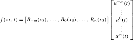 \begin{align} f(x_3,t)=\begin{bmatrix} B_{-m}(x_3),\ldots, B_{0}(x_3),\ldots, B_m(x_3) \end{bmatrix}\begin{bmatrix} u^{-m}(t) \\ \vdots \\ u^0(t) \\ \vdots \\ u^{m}(t) \end{bmatrix} \end{align}
represents the global field formed by aggregating the
 $B_i$
(with either
 $B_i=B_{u^i}$
or
 $B_i=B_{w^i}$
; here we dropped
 $u/w$
for clarity) at the various spanwise locations and is
 $L_{x_3}$
-periodic. Introducing the truncated Fourier decompositions in
 $x_3$
of
 $f$
and
 $B_i$
, we obtain
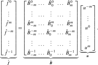 \begin{align} \underbrace {\begin{bmatrix} \hat {f}^0\\[5pt] \vdots \\[5pt] \hat {f}^m\\[5pt] \hat {f}^{-m}\\[5pt] \vdots \\[5pt] \hat {f}^{-1} \end{bmatrix}}_{\hat {\boldsymbol{f}}} =\underbrace {\begin{bmatrix} \hat {B}^0_{-m} & \ldots & \hat {B}^0_{0} & \ldots & \hat {B}^0_{m}\\[5pt] \vdots & \ldots & \vdots & \ldots & \vdots \\[5pt] \hat {B}^m_{-m} & \ldots & \hat {B}^m_{0} & \ldots & \hat {B}^m_{m}\\[5pt] \hat {B}^{-m}_{-m} & \ldots & \hat {B}^{-m}_{0} & \ldots & \hat {B}^{-m}_{m}\\[5pt] \vdots & \ldots & \vdots & \ldots & \vdots \\[5pt] \hat {B}^{-1}_{-m} & \ldots & \hat {B}^{-1}_{0} & \ldots & \hat {B}^{-1}_{m} \end{bmatrix}}_{\hat {\boldsymbol{B}}}\underbrace {\begin{bmatrix} u^{-m} \\[5pt] \vdots \\[5pt] u^{0} \\[5pt] \vdots \\[5pt] u^{m} \end{bmatrix}}_{\boldsymbol{u}}. \end{align}
Using the Poisson summation formula and the effect of a translation on a Fourier transform, we find that
 \begin{align} B_i(x_3)=\sum _{p=-\infty }^\infty b(x_3-i\varDelta _{x_3}+pn\varDelta _{x_3})\quad \Rightarrow \quad \hat {B}^{k}_i=\dfrac {1}{n\varDelta _{x_3}}\hat {b}(k\beta /n)\omega _n^{ik}, \end{align}
where a localized source
 $b$
is taken as either
 $b=b_w$
or
 $b=b_u$
and where
 $\hat {b}(\xi )=\int _{-\infty }^\infty b(x_3)\mathrm{e}^{-{i}\xi x_3}\,\mathrm{d}x_3$
is the Fourier transform. Hence,
 $B_i(x_3)$
represents the
 $L_{x_3}$
-periodic extension of a source
 $b$
loacted at
 $x_3=i\varDelta _{x_3}$
. We have
 $b_w(x_3)=\delta _{\textit{Dirac}}(x_3)$
so for the noise sources the Fourier coefficients
 $\hat {b}_w(k\beta /n)$
are all identically equal to unity. The actuator field
 $b_u(x_3)$
is a Gaussian, and since the Fourier transform of a Gaussian is also a Gaussian,
 $\hat {b}_u(k\beta /n)$
is a real-valued function of
 $k^2$
. In both cases, we may write
 $\hat {\boldsymbol{B}}=\boldsymbol{D}\!\boldsymbol{F}_n$
where
 $\boldsymbol{D}$
is a diagonal matrix with
 $\boldsymbol{D}_{kk}={d}(k^2)\in \mathbb{R}$
, and
 $\boldsymbol{F}_n$
is the DFT matrix. Since
 $\hat {\boldsymbol{u}}=\boldsymbol{F}_n\boldsymbol{u}$
, we therefore have
 $\hat {\boldsymbol{f}}=\boldsymbol{D}\hat {\boldsymbol{u}}$
(and similarly for
 $\boldsymbol{w}$
, except the diagonal is constant). In other terms there is a one-to-one mapping
 $\hat {f}^k=d(k^2)\hat {u}^k$
between transverse Fourier modes
 $\hat {f}^k$
and inputs
 $\hat {u}^k$
and as a result
 \begin{align} \hat {\boldsymbol{f}}^k_{\boldsymbol{\eta }}(t)=\boldsymbol{F}(x_1,x_2)d(k^2)\hat {u}^k(t). \end{align}
Similarly, there exists a real field
 $\boldsymbol{C}(x_1,x_2)$
such that
 \begin{align} y^i(t)=\boldsymbol{C}(x_1,x_2)\boldsymbol{\cdot }\boldsymbol{\eta }(x_1,x_2,i\varDelta _{x_3},t) \end{align}
so
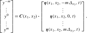 \begin{align} \begin{bmatrix} y^{-m}\\\vdots \\ y^{0}\\ \vdots \\y^{m} \end{bmatrix}=\boldsymbol{C}(x_1,x_2)\boldsymbol{\cdot }\begin{bmatrix} \boldsymbol{\eta }(x_1,x_2,-m\varDelta _{x_3},t)\\\vdots \\ \boldsymbol{\eta }(x_1,x_2,0,t)\\\vdots \\ \boldsymbol{\eta }(x_1,x_2,m\varDelta _{x_3},t) \end{bmatrix}, \end{align}
and applying the DFT matrix to the left, we find
 \begin{align} \hat {y}^k=\boldsymbol{C}(x_1,x_2)\boldsymbol{\cdot }\hat {\boldsymbol{\eta }}^k(x_1,x_2,t). \end{align}
Combining (B3), (B7) and (B10), we find that the transfer
 \begin{align} \hat {T}^k_{yu}=\boldsymbol{C}\boldsymbol{\cdot }\big(s\boldsymbol{I}-\hat {\boldsymbol{A}}^k_{\boldsymbol{\eta }\boldsymbol{\eta }} \big)^{-1}\boldsymbol{F}d(k^2) \end{align}
admits a real state-space realization
 $(\hat {\boldsymbol{A}}_{\boldsymbol{\eta }\boldsymbol{\eta }}^k,\boldsymbol{F}d(k^2),\boldsymbol{C}\boldsymbol{\cdot },0)$
. As a consequence, the impulse response from
 $\hat {u}^k$
to
 $\hat {y}^k$
is real despite the inputs and outputs being complex, and we may therefore apply standard identification and synthesis methods in the wavenumber space. Moreover, since the transfer function depends on
 $k^2$
, we have
 \begin{align} \hat {T}^{-k}_{yu}=\hat {T}^k_{yu}, \end{align}
therefore we only need to perform synthesis and identification for
 $k=0,\ldots, m$
. The same properties hold for the other transfer functions, i.e.
 $\hat {T}^k_{yw}$
,
 $\hat {T}^k_{zw}$
,
 $\hat {T}^k_{zu}$
.
Appendix C. Analysis of the synthesis results on the ROMs
The results of the six controllers
 $\hat {K}^{k}$
on the ROMs are analysed here. The figure 23(a) shows the magnitude of
 $\hat {K}^k\hat {S}^{k}$
for the two steps of the algorithmic procedure. As expected, minimizing
 $\|\hat {K}^k\hat {S}^{k}\|_2$
in step 2 also led to decrease
 $\|\hat {K}^k\hat {S}^{k}\|_\infty$
, thereby contributing to stability robustness, particularly at low and high frequencies. The actuator activity
 $\|\boldsymbol{K}\boldsymbol{S}\|^2_2$
at the end of step 2 is approximately 3.6 times lower than after step 1. This allows a stronger performance robustness to white noise corrupting estimation sensors (see Appendix D), and this without impacting nominal performance as, in the bandwidth of the first mode (
 $F \sim [0.02,0.2]$
) and second Mack mode (
 $F \sim [0.2,0.3]$
), the actuator activities resulting from step 1 and 2 are equivalent. All the controllers have the roll-off of
 $-20$
dB per decade at high frequencies due to their strictly proper structure.
Nominal performance on the ROMs for each spanwise mode
 $k$
normalized by the weightings used in step 1 of the algorithmic procedure (i.e. their respective uncontrolled values
 $\|\boldsymbol{T}_{\!\boldsymbol{z}_4\boldsymbol{w}}\|_{2}$
and
 $\|\boldsymbol{T}_{\!\boldsymbol{z}_{1:3}\boldsymbol{w}}\|_{2}$
approximated by the six spanwise modes used in the synthesis).
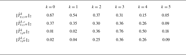
Table 2. Long description
The table presents nominal performance on ROMs for each spanwise mode normalized by the weightings used in step 1 of the algorithmic procedure. It has four rows and six columns. The columns are labeled with k values ranging from 0 to 5. The rows are labeled with different performance metrics. The values in the table are as follows: Row 1: k = 0, 0.67; k = 1, 0.54; k = 2, 0.37; k = 3, 0.31; k = 4, 0.15; k = 5, 0.05. Row 2: k = 0, 0.37; k = 1, 0.35; k = 2, 0.30; k = 3, 0.36; k = 4, 0.26; k = 5, 0.09. Row 3: k = 0, 0.01; k = 1, 0.02; k = 2, 0.36; k = 3, 0.76; k = 4, 0.50; k = 5, 0.18. Row 4: k = 0, 0.02; k = 1, 0.04; k = 2, 0.25; k = 3, 0.36; k = 4, 0.26; k = 5, 0.09.
(a) Gain of
 $\hat {K}^k\hat {S}^{k}$
for the two minimization steps. (b) Nyquist plot of the loop gain
 $-\hat {T}^k_{yu}\hat {K}^{k}$
at the end of the step 2.
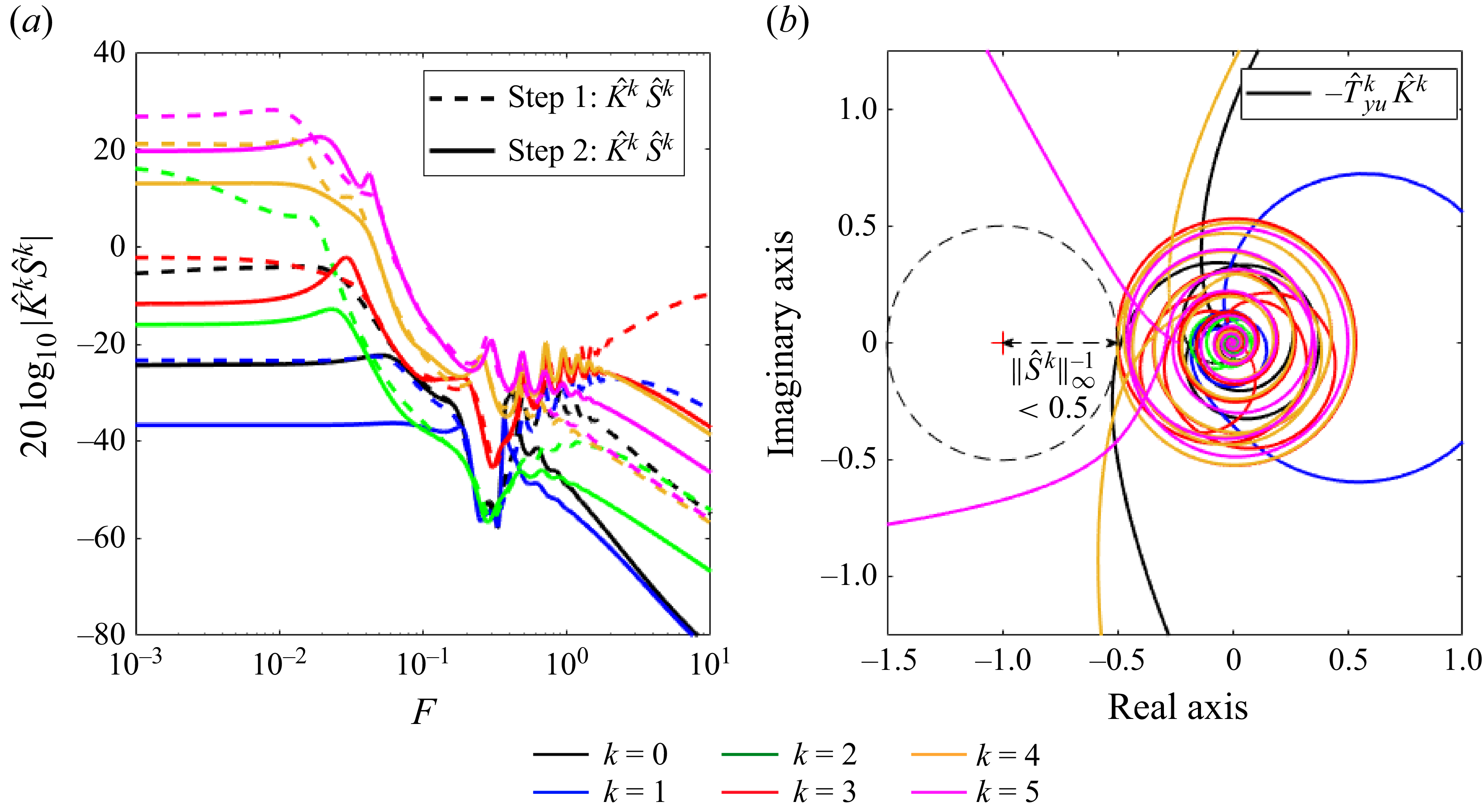
The Nyquist plots of the SISO loop gains
 $-\hat {T}_{yu}^k\hat {K}^k$
after step 2 is plotted in figure 23(b). The minimal distance between the Nyquist plots and the critical point (−1,0) (red cross) at which a closed-loop becomes unstable is greater than 0.5 for all loop gains, which obeys logically the constraint imposed in the CMPs (see § 6.1). Some controllers are even farther away from the critical point and have higher stability margins: for example
 $\|\hat {S}^{1}\|^{-1}_{\infty }=0.82$
which means that the controller
 $\hat {K}^{1}$
will be guaranteed stable up to
 $82\,\%$
of relative model error
 $\hat {\varDelta } ^{1}$
(e.g. combination of pure gain and phase shifts) on
 $\hat {T}_{yu}^{1}$
. Concerning the nominal performance evaluated on the ROMs, it is summarized in table 2. The weightings privileges pressure disturbance rejection over velocity disturbance rejection for the first two modes
 $k=0$
and
 $k=1$
as
 $\|\hat {T}^{k,c}_{\boldsymbol{z}_{1:3}w}\|_{2}\gt \|\hat {T}^{k,c}_{z_4w}\|_{2}$
. Due to the ‘
 $\text{minimize}\ \mathrm{max}$
’ problem, the algorithm seeks in priority to minimize the pressure perturbations and even amplifies the velocity perturbations compared with the uncontrolled case for these first two spanwise modes. Hence, an effect similar to the waterbed effect appears as the reduction of the amplitude of some frequencies leads to the amplification of other ones (Skogestad & Postlethwaite Reference Skogestad and Postlethwaite2005; Nibourel et al. Reference Nibourel, Leclercq, Demourant, Garnier and Sipp2023). Both pressure and velocity disturbances are reduced for
 $k=2$
. For the last three modes
 $k=3$
,
 $k=4$
and
 $k=5$
, the weightings lead to privilege velocity disturbance rejection while pressure perturbations are amplified until reaching
 $\|\hat {T}^{k,c}_{\boldsymbol{z}_{1:3}w}\|_{2}\simeq \|\hat {T}^{k,c}_{z_4w}\|_{2}$
where it is no longer possible to reduce one without degrading the other.
Appendix D. Robustness to noisy estimation sensors
Firstly, all the estimation sensors
 $y^i$
are corrupted by uncorrelated white Gaussian noises
 $n^i$
and by the same amount of noise (
 $50\,\%$
of the r.m.s. value without control of
 $y^i$
, i.e. SNR of 2). The PSD of the noisy estimations sensors
 $y^i$
(red line) is very far from that of the ideal sensors (blue line) in low and high frequencies (see figure 24
a) because as
 $n^i$
is a white noise, the ratio
 $\varPhi _{y^i}/\varPhi _{n^i}$
(with
 $\varPhi$
the PSD) is low where the ideal signal power is low. Conversely,
 $\varPhi _{y^i}/\varPhi _{n^i}$
is large where the ideal signal power is large (
 $F\sim [0.06,0.35]$
) and the PSD of the noisy sensors is similar to that of the ideal sensors. The PSD of the actuator signals for corrupted
 $\boldsymbol{y}$
differs from that of ideal
 $\boldsymbol{y}$
also in low and high frequencies because
 $\boldsymbol{u}(iF)=\boldsymbol{K}(iF)\boldsymbol{y}(iF)$
(see figure 24
b). The maximum along the wall-normal direction of
 $\lt v'_{x_1,\textit{rms}}\gt _{x_3}$
slightly differs between the ideal and noisy estimation sensor cases (see figure 24
c). Yet, except a bump near the streamwise actuator position due to the higher energy injection in low frequencies, the quantity
 $\mathrm{max}_{x_2}\ \lt v'_{x_1, {rms}}\gt _{x_3}$
stays below the uncontrolled curve all along the domain. For the quantity
 $\mathrm{max}_{x_2}\ \lt p'_{\textit{rms}}\gt _{x_3}$
, the noisy sensors lead to a stronger acoustic wave (see figure 24
d). Downstream of this acoustic wave, the attenuation of disturbances with noisy sensors is equal to that with ideal ones. This is because the frequencies of the second Mack mode to be controlled (
 $F \sim [0.2,0.3]$
) are not impacted by the white noises
 $\boldsymbol{n}$
as
 $\varPhi _{y^i}/\varPhi _{n^i}$
is the most important in this bandwidth, unlike the frequencies of the first instability mode to be controlled (
 $F \sim [0.02,0.2]$
) where this ratio is weaker involving higher variations between the ideal and noisy cases for the quantities related to this first mode (e.g. the velocity field at
 $x_{2,\textit{GIP}}$
). Note that if a strictly proper structure for
 $\hat {K}^{k}$
had not been imposed in the synthesis and the minimization of
 $\|\hat {K}^k\hat {S}^{k}\|_2$
not realized in step 2 of the CMPs, the power of the actuator signals would be much higher in high and low frequencies and the intensities of the velocity bump and the acoustic wave would have been even more important.
In all panels, controlled systems with ideal and noisy estimation sensors
 $\boldsymbol{y}$
are represented by blue and red lines, respectively. The PSD of (a)
 $y^0$
and (b)
 $u^0$
. Evolution of (c)
 $\max _{x_2} \lt v'_{x_1, {rms}}\gt _{x_3}$
and (d)
 $\max _{x_2} \lt p'_{\textit{rms}}\gt _{x_3}$
. For vertical lines in (c) and (d), same caption as in figure 16.
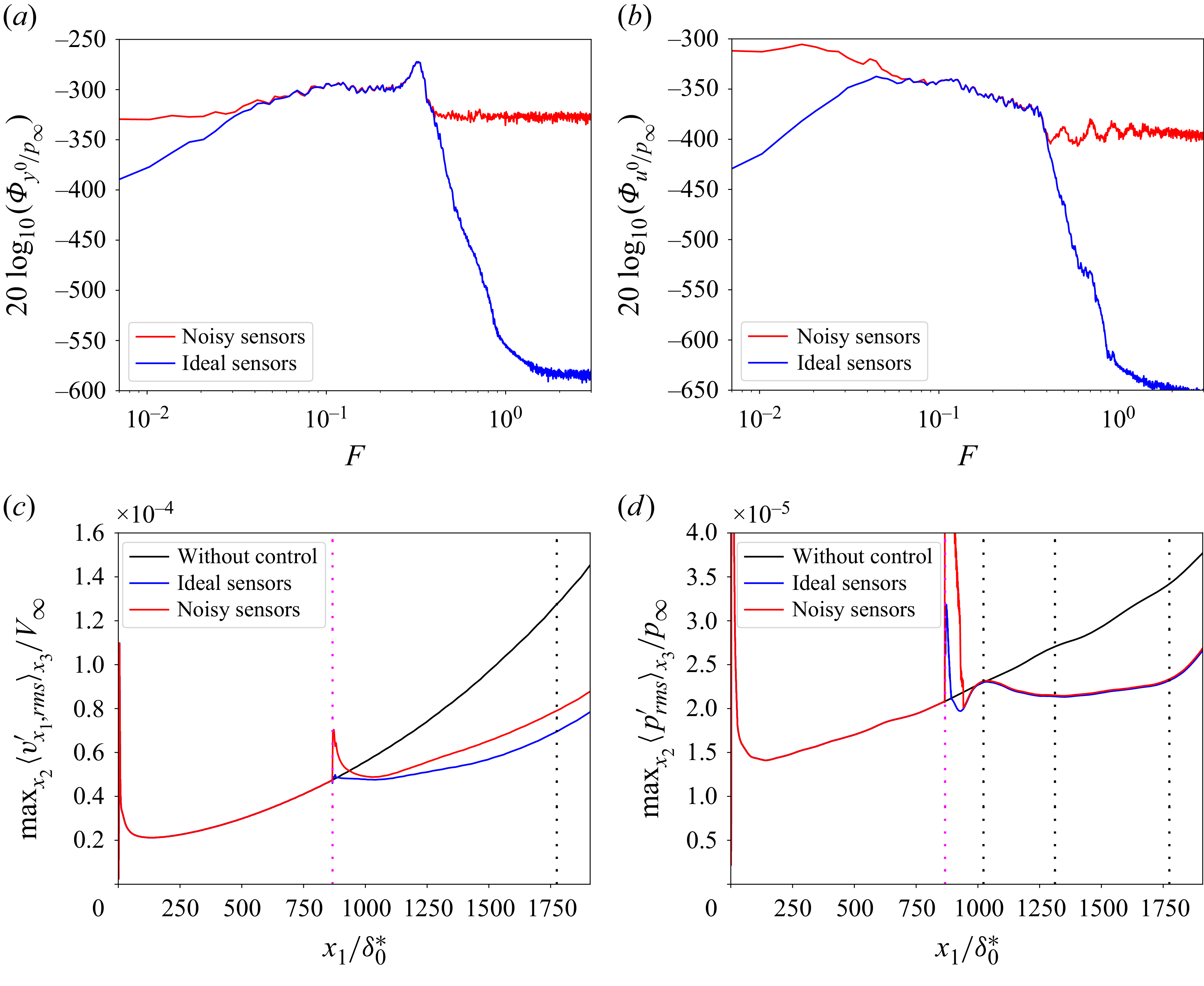
Figure 24. Long description
The image contains four panels, each depicting different graphs related to the behavior of controlled systems with ideal and noisy estimation sensors. Panel A: A line graph showing the power spectral density (PSD) of a variable with the x-axis labeled F and the y-axis labeled 20 log10(Phi_y0/p_infinity). The graph includes two lines, one red representing noisy sensors and one blue representing ideal sensors. Panel B: Another line graph showing the PSD of a different variable with the same axis labels as Panel A. The graph also includes two lines, one red for noisy sensors and one blue for ideal sensors. Panel C: A line graph showing the evolution of a variable with the x-axis labeled x1/delta0* and the y-axis labeled Max2(u_rms/x3)/V_infinity. The graph includes three lines, one black for without control, one blue for ideal sensors, and one red for noisy sensors. Vertical lines are present at specific points. Panel D: A line graph showing the evolution of another variable with the x-axis labeled x1/delta0* and the y-axis labeled Max2(p_rms/x3)/p_infinity. The graph includes three lines, one black for without control, one blue for ideal sensors, and one red for noisy sensors. Vertical lines are present at specific points.
Considering white noises
 $\boldsymbol{n}$
is the most conservative approach when the type of noise corrupting the sensors
 $\boldsymbol{y}$
is unknown. Some sensors may be noisy only in high frequencies in a realistic set-up (Lugrin et al. Reference Lugrin, Nicolas, Severac, Tobeli, Beneddine, Garnier, Esquieu and Bur2022). A high-pass filter of order 12 with a cutoff frequency
 $F=0.38$
is applied to the white Gaussian noises
 $n^i$
previously used. Hence, the estimation sensors are now corrupted by coloured noises outside the bandwidth of the first and second instability modes to be controlled. Different ideal signal-to-noise ratios for these coloured noises are evaluated:
 $\mathrm{SNR}_1\simeq 2.08$
(denoted ‘low noise’),
 $\mathrm{SNR}_2\simeq 1.04$
(denoted ‘medium noise’) and
 $\mathrm{SNR}_3\simeq 0.52$
(denoted ‘high noise‘). The PSD of the estimation and actuator signals are corrupted only in high frequencies with these coloured noises (see figure 25
a,b). The velocity disturbance rejection is as in the ideal sensor case even in the high noise
 $\mathrm{SNR}_3\simeq 0.52$
case (see figure 25
c). The velocity bump that was present in the case of white noises is no longer present while the
 $\mathrm{SNR}$
is lower in the medium and high noise cases than in the previous white noise case: this velocity bump was clearly due to the low-frequency actuator activity which took important values when estimation sensors were corrupted by white noises. The pressure disturbance rejection is also equivalent to the ideal sensor case except in the acoustic wave region (see figure 25
d): the acoustic wave intensity increases with the intensity of the coloured noise but remains much lower than in the white noise case despite lower signal-to-noise ratios.
Estimation sensors
 $\boldsymbol{y}$
are corrupted by different levels of coloured noises. The PSD of (b)
 $y^0$
and (c)
 $u^0$
. Evolution of (d)
 $\max _{x_2} \lt v'_{x_1, {rms}}\gt _{x_3}$
and (e)
 $\max _{x_2} \lt p'_{\textit{rms}}\gt _{x_3}$
. For vertical lines in (d) and (e), same caption as in figure 16.
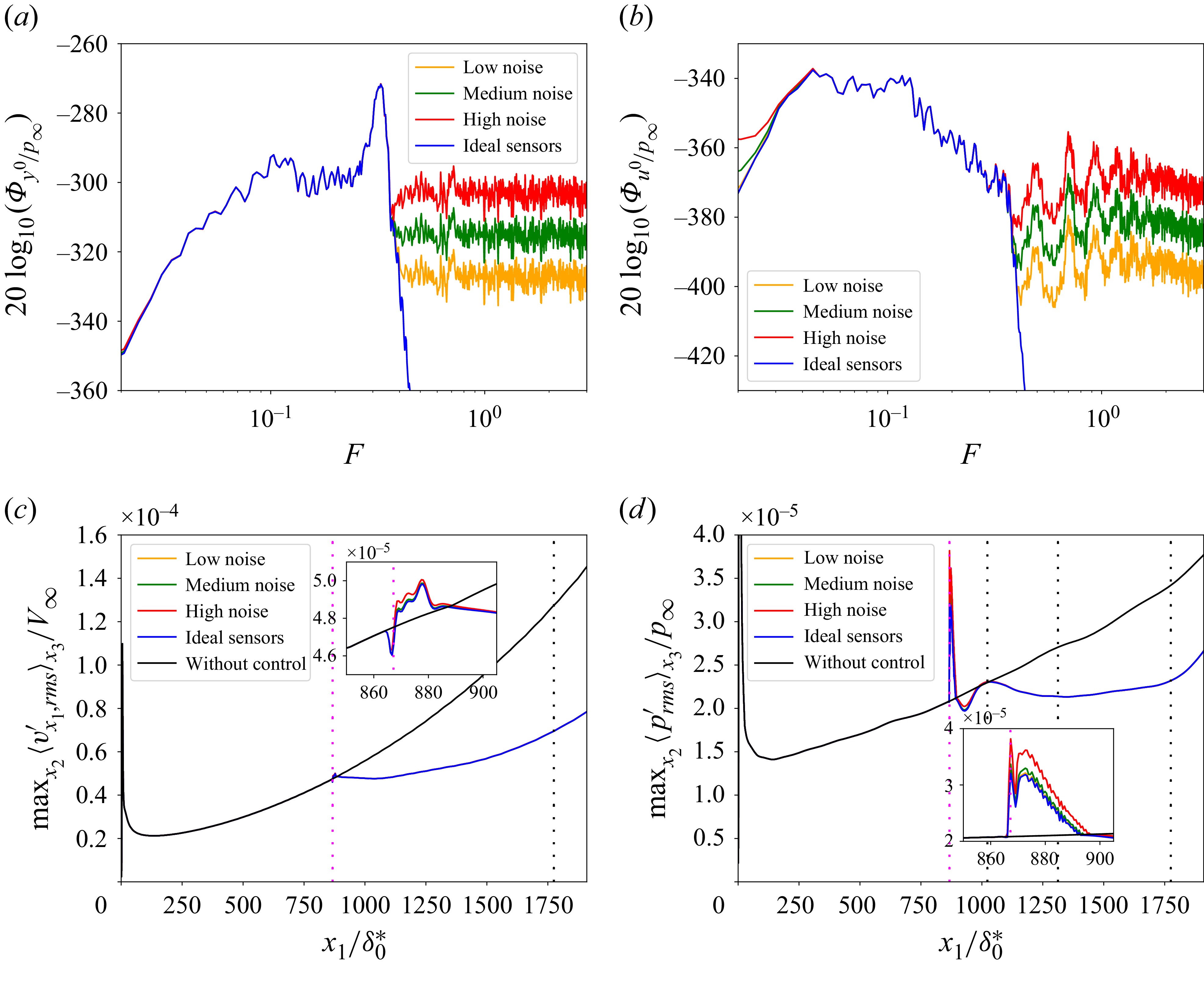
If even noisier sensors were used or if the velocity/acoustic bumps prevented delaying transition to turbulence, it would be enough to reduce more the actuator activity
 $\hat {K}^k\hat {S}^{k}$
in the CMPs (especially in low frequencies) by relaxing the constraints related to nominal performance.
Appendix E. Robustness to nonlinearities
All the results presented in §§ 5 and 7.1 were for
 $w^i(t)$
of sufficiently low value to obtain perturbations which remain in the linear regime until the end of the domain. Even for the transition to turbulence case § 7.2, the level of nonlinearities were low at the streamwise position of the actuators (actuators built from linear tools). This appendix assesses the robustness of the control law to nonlinearities by employing noise source levels that result in significant amplitude disturbances at the actuator’s streamwise position.
Two variances for the exogenous noise sources leading to nonlinear growth in the domain are tested:
 $\mathrm{Var}[w^i]=1$
and
 $\mathrm{Var}[w^i]=25$
. Note that the variance used in the linearized DNS was
 $\mathrm{Var}[w_{\textit{linear}}^i]=0.0016$
. The fluctuations of the estimation sensors are up to
 $0.19\,\%$
and
 $1\,\%$
of
 $p_\infty$
when
 $\mathrm{Var}[w^i]=1$
and
 $\mathrm{Var}[w^i]=25$
, respectively. At the streamwise position of the estimation sensors, the velocity fluctuations are up to
 $0.38\,\%$
and
 $2\,\%$
of
 $V_{\infty }$
when
 $\mathrm{Var}[w^i]=1$
and
 $\mathrm{Var}[w^i]=25$
, respectively. The control law still reduces significantly both velocity and pressure disturbances when
 $\mathrm{Var}[w^i]=1$
, which is considered as a weakly nonlinear case as the results are close to the linear ones all along the domain (see figure 26
a,b). When
 $\mathrm{Var}[w^i]=25$
(see figure 26
c,d), the perturbation amplitude is such that the disturbances are moderately nonlinear at
 $x_{1,\boldsymbol{u}}$
before being strongly nonlinear at the end of the domain. For this stronger nonlinear case, the control law still manages to maintain some performance by staying below
 $\max _{x_2} \lt v'_{x_1,\textit{rms}}\gt _{x_3}$
of the uncontrolled system all along the domain but the mitigation of pressure disturbances is no longer effective. Thus, the control law designed from linear tools appears to be robust to nonlinearities in terms of velocity perturbation rejection while the performance in terms of pressure perturbation rejection drops when the nonlinear effects are too large. Perhaps reducing velocity fluctuations (while not decreasing pressure fluctuations) is sufficient to delay the transition to turbulence. Yet, as this has not been investigated in more detail since it was considered outside the scope of the article, we chose to keep low nonlinearities at the actuator level to control both velocity and pressure fluctuations.
For exogenous noise sources with (a,b)
 $\mathrm{Var}[w^i]=1$
and (c,d)
 $\mathrm{Var}[w^i]=25$
, evolution of (a,c)
 $\max _{x_2} \lt v'_{x_1,\textit{rms}}\gt _{x_3}$
and (b,d)
 $\max _{x_2} \lt p'_{\textit{rms}}\gt _{x_3}$
. The linear cases (dashed lines) are rescaled by multiplying their results by
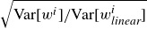 $\sqrt {\mathrm{Var}[w^i]/\mathrm{Var}[w_{\textit{linear}}^i]}$
for comparison. For vertical lines, same caption as in figure 16.
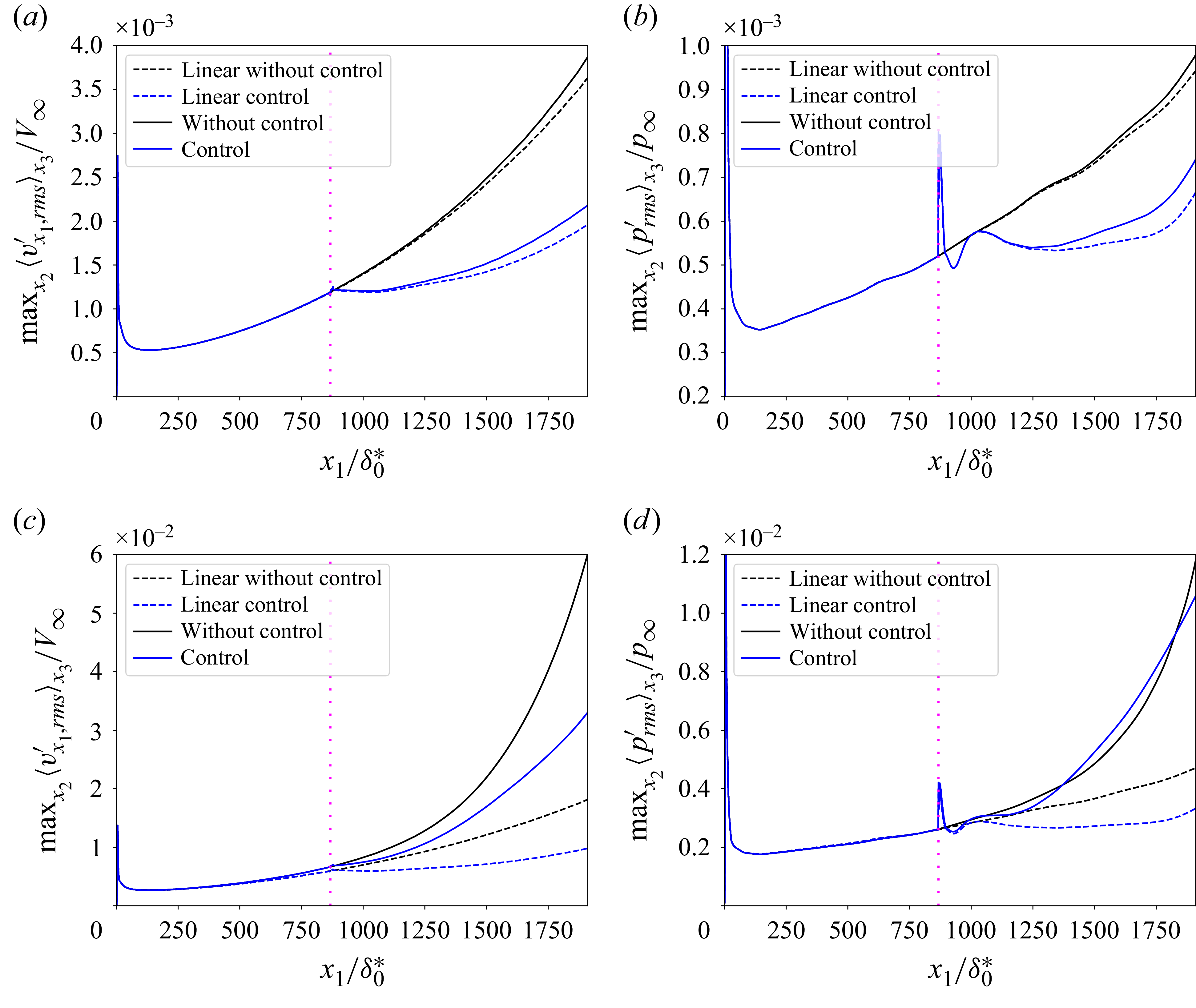
Figure 26. Long description
The image contains four line graphs labeled (a), (b), (c), and (d). Each graph compares the effects of control on turbulence transition in boundary layer flows. Panel A: This line graph shows the maximum value of the root mean square of velocity fluctuations normalized by a reference velocity. The x-axis is labeled x1/delta0* and ranges from 0 to 1750. The y-axis is labeled Max_x2(v’_rms_x1)/V_infinity and ranges from 0 to 4.0 times 10^−3. The graph includes four lines: dashed black for linear without control, dashed blue for linear control, solid black for without control, and solid blue for control. Panel B: This line graph shows the maximum value of the root mean square of pressure fluctuations normalized by a reference pressure. The x-axis is labeled x1/delta0* and ranges from 0 to 1750. The y-axis is labeled Max_x2(p’_rms_x1)/p_infinity and ranges from 0 to 1.0 times 10^−3. The graph includes four lines: dashed black for linear without control, dashed blue for linear control, solid black for without control, and solid blue for control. Panel C: This line graph shows the maximum value of the root mean square of velocity fluctuations normalized by a reference velocity. The x-axis is labeled x1/delta0* and ranges from 0 to 1750. The y-axis is labeled Max_x2(v’_rms_x1)/V_infinity and ranges from 0 to 6.0 times 10^−2. The graph includes four lines: dashed black for linear without control, dashed blue for linear control, solid black for without control, and solid blue for control. Panel D: This line graph shows the maximum value of the root mean square of pressure fluctuations normalized by a reference pressure. The x-axis is labeled x1/delta0* and ranges from 0 to 1750. The y-axis is labeled Max_x2(p’_rms_x1)/p_infinity and ranges from 0 to 1.2 times 10^−2. The graph includes four lines: dashed black for linear without control, dashed blue for linear control, solid black for without control, and solid blue for control.


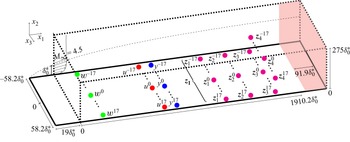
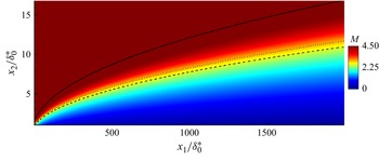
 x3
 δ
 x2,GIP
 δ∗
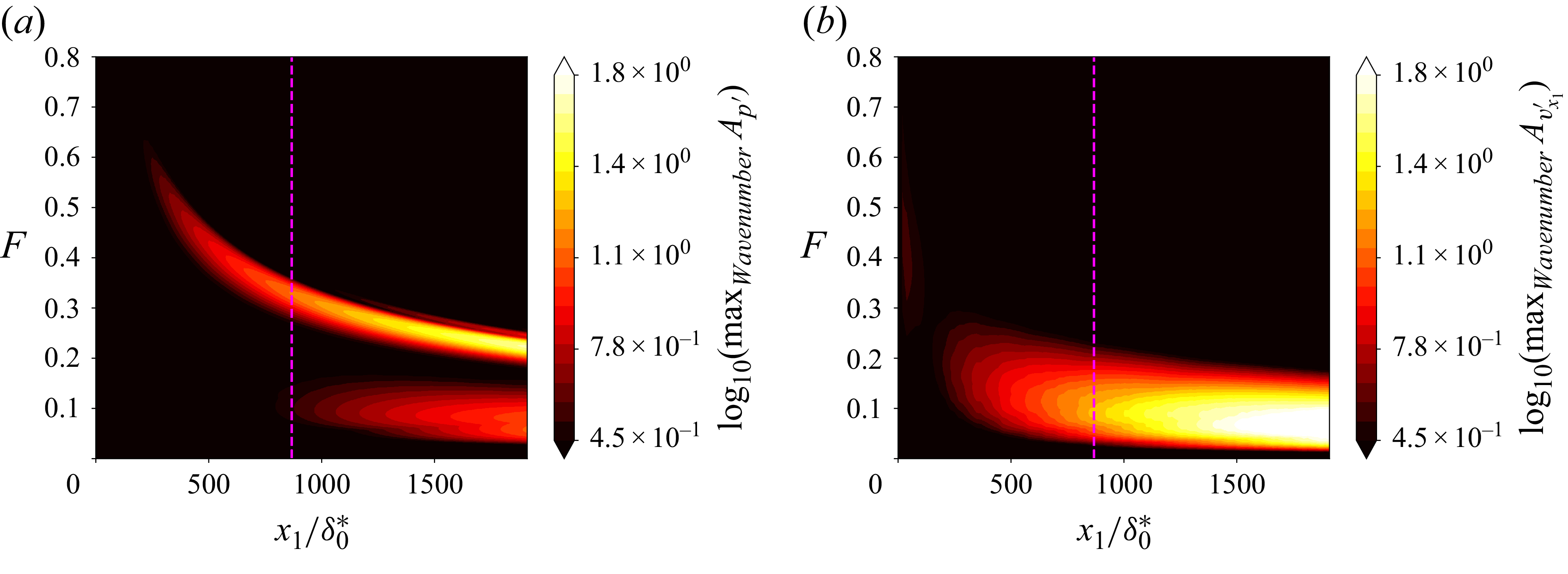
 x2=0
 x2=x2,GIP

 δ0∗
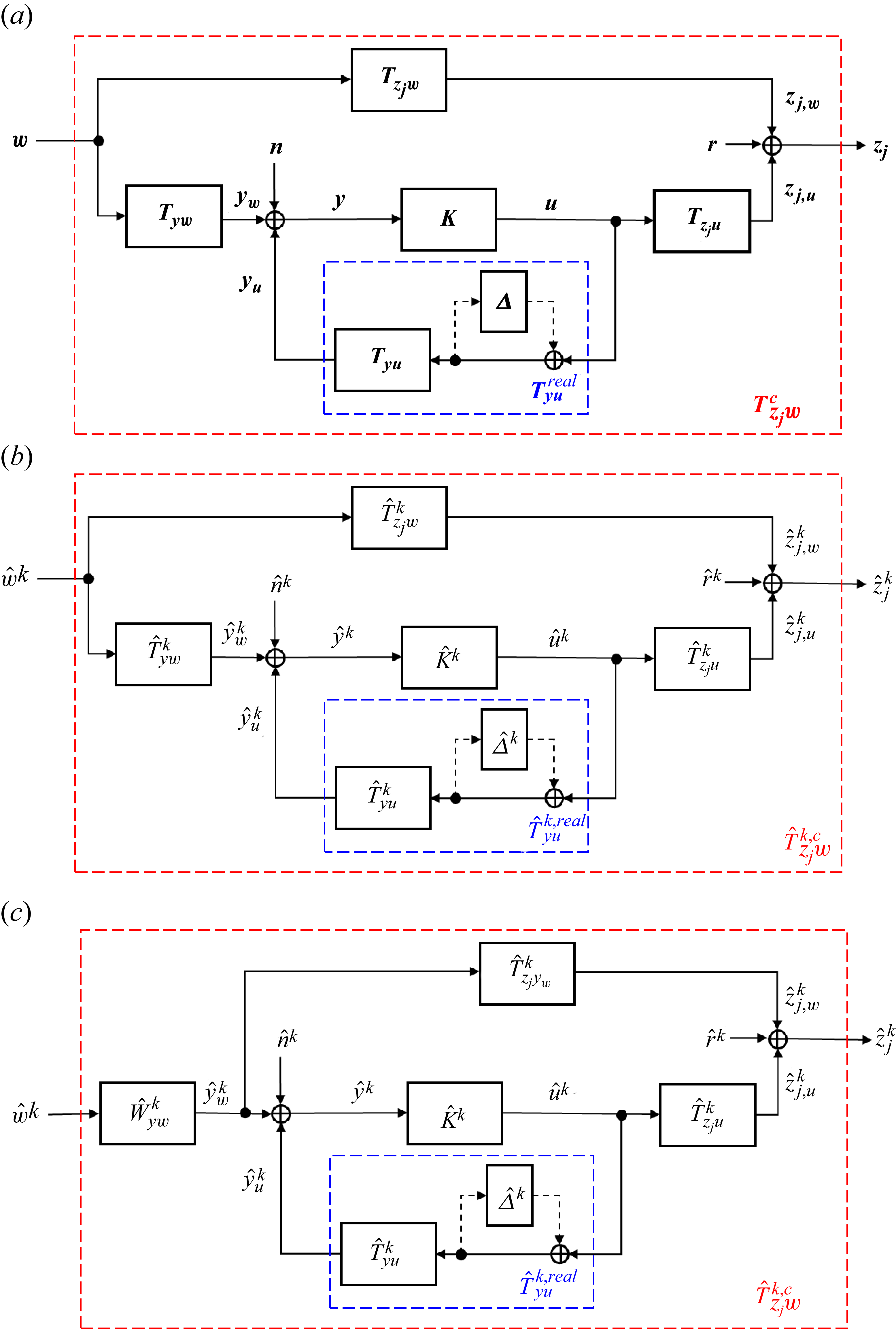
 Δ
 n
 n×n
 n=2m+1
 m+1
 W^ywk
 T^zjywk
 w^k
 z^jk(t):=z^jk(t+τzjyw)
 τzjyw
 yw
 zj
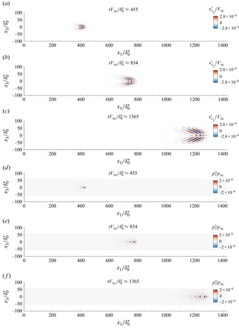
 tV∞/δ0∗=
 455
 834
 1365
 w0
 t=0
 x2,GIP
 x2=1.99δ0∗
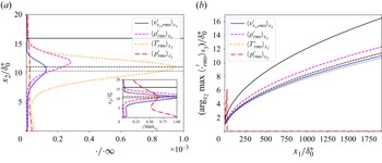
 x1=1766.7δ0∗
 argx2 max
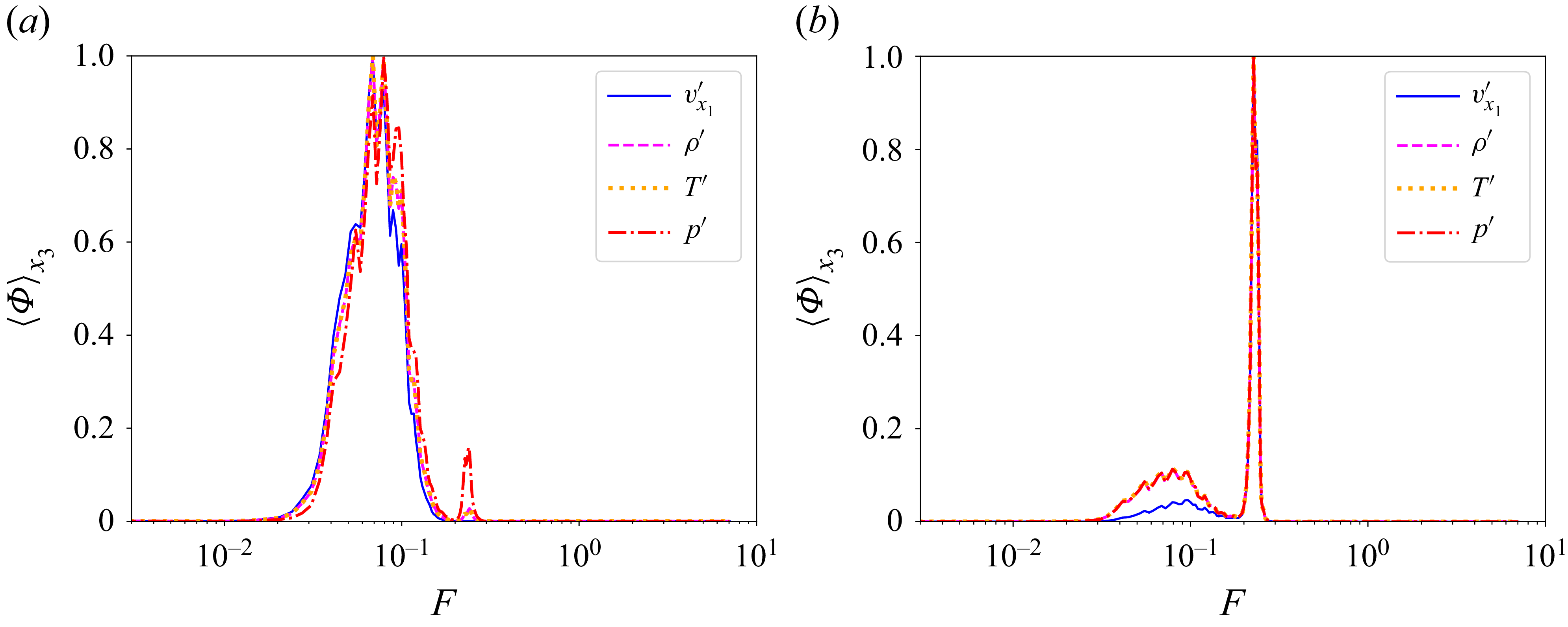
 x1=1775δ0∗
 x2,GIP
 x2=0.015δ0∗
 x2,GIP
 35
 wi
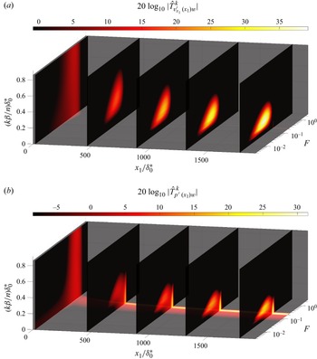
 T^ϕ(x1)wk
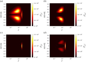
 u^k
 w^k
 z^3k
 z^4k
 x2,GIP
 T^z4uk
 T^z4wk
 T^z3uk
 T^z3wk
 |k|=17
 (|k|β/n)δ0∗≃0.92
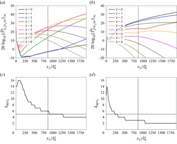
 ‖T^ϕ(x1)wk‖∞
 |k|⩽8
 k90%
 90%
 ‖Tϕ(x1)w‖2
 ϕ(x1)
 x2,GIP
 x1,u
 |k|≤5
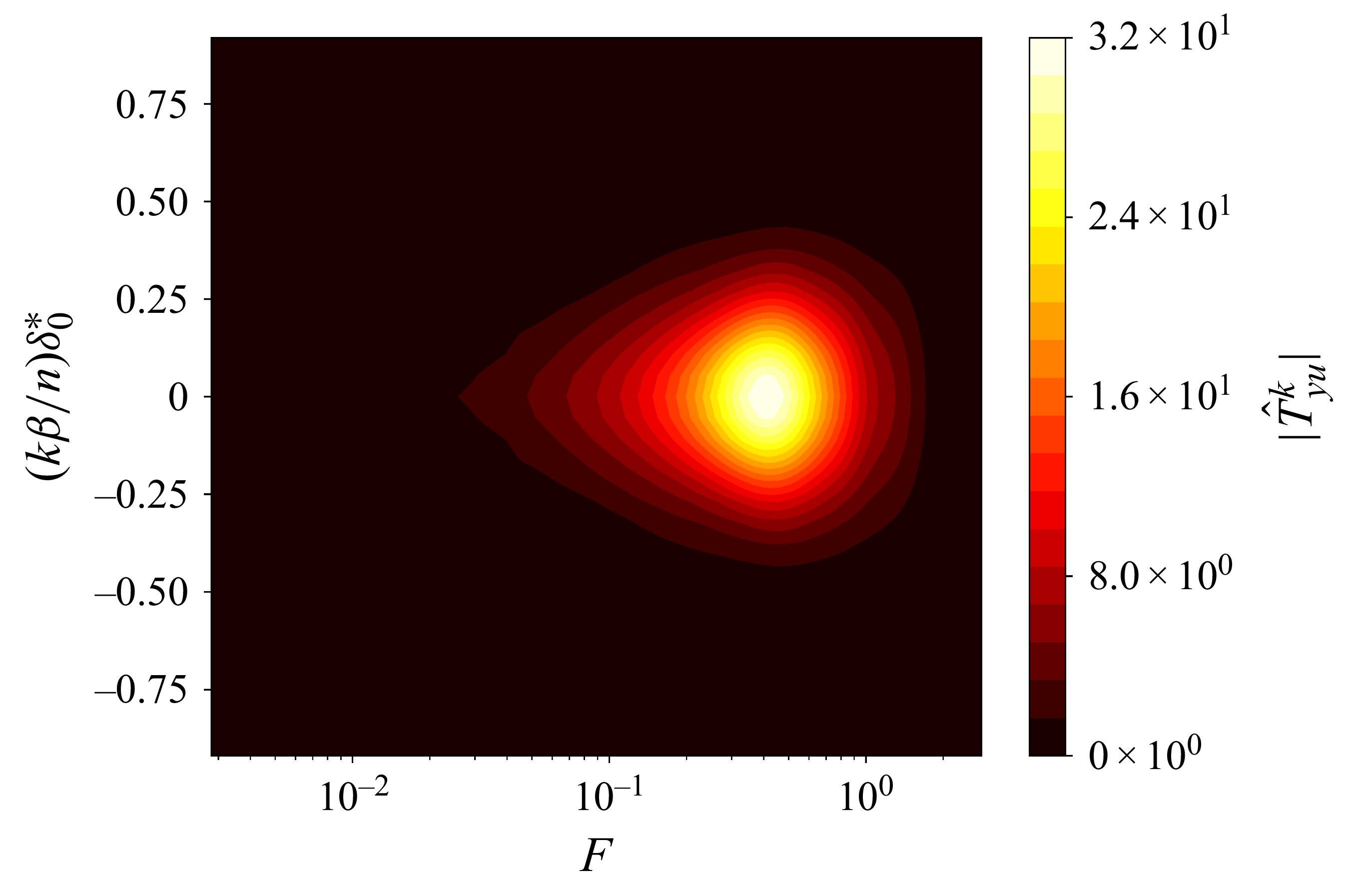
 T^yuk
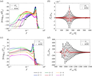
 W^ywk
 T^z3ywk
 T^z3ywk
 τzjywV∞/δ0∗≃892
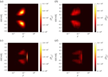
 z4
 z3
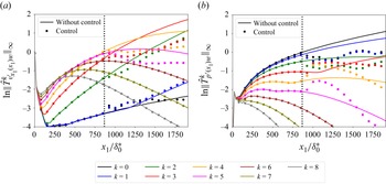
 ‖T^ϕ(x1)wk‖∞
 |k|⩽8
 ϕ(x1)
 x2=x2,GIP
 ‖T^ϕ(x1)wk‖∞
 ‖T^vx1′(x1,u)w4‖∞
 ‖T^p′(x1,u)w0‖∞
 N
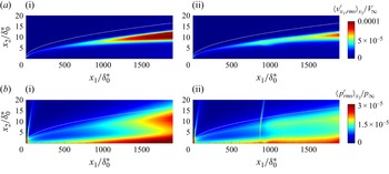
 vx1,rms′
 prms′
 δ
 x2,GIP
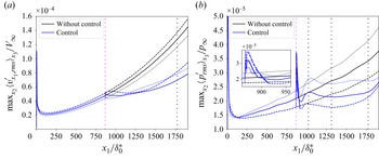
 maxx2x3
 maxx2x3
 V∞
 ±2.5%
 +2.5%
 −2.5%
 y
 zj
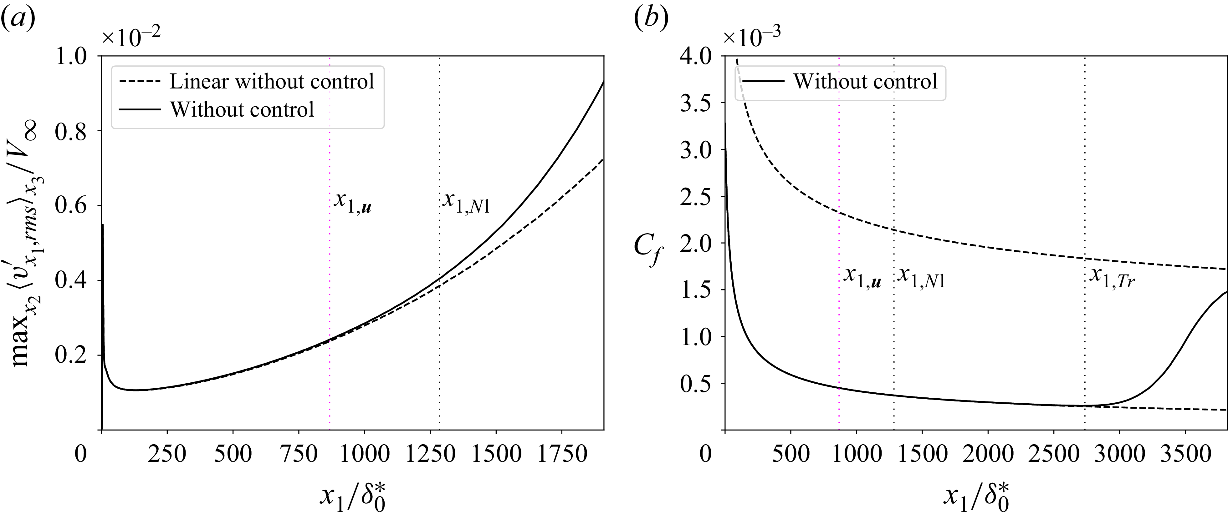
 Var[wi]=4
 maxx2x3
 Cf
 Var[wi]/Var[wlineari]
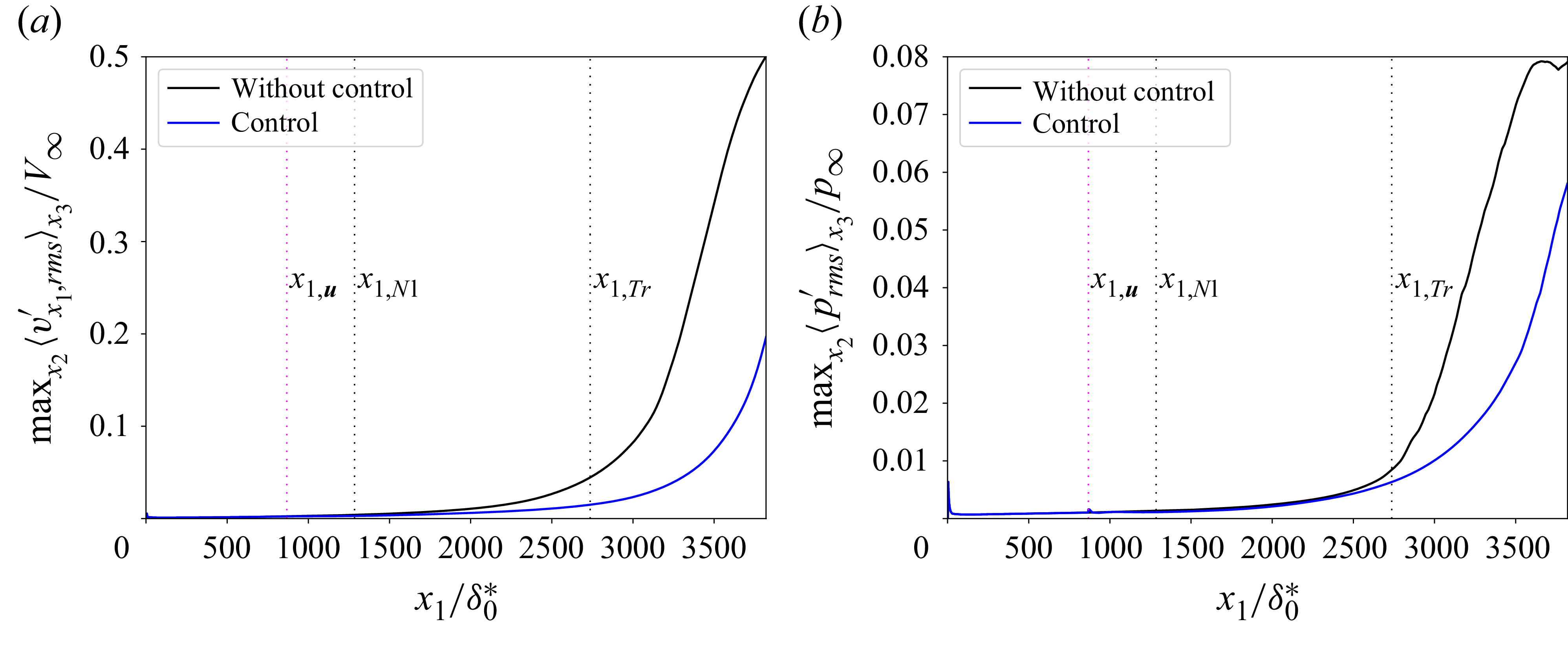
 maxx2<.rms>x3
 vx1′
 p′
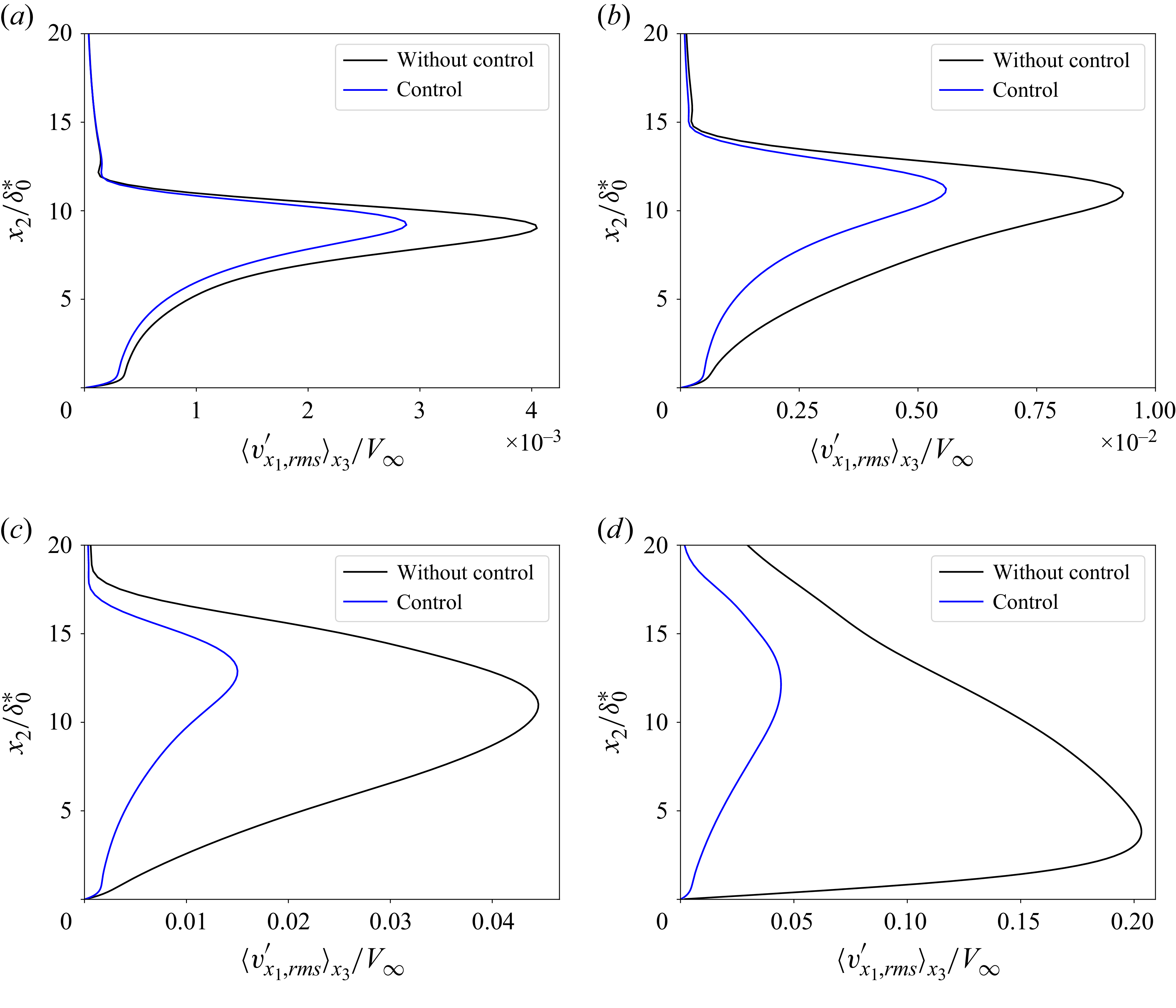
 x3
 x1=x1,Nl
 x1=1910.2δ0∗
 x1=x1,Tr
 x1=3300.5δ0∗
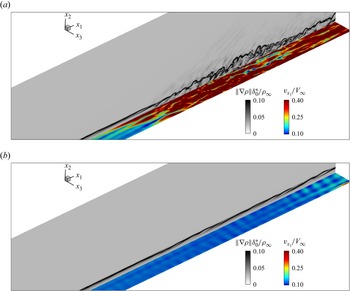
 x1x3
 x2=1.99δ0∗
 x1x2
 x3=0
 2939.7δ0∗
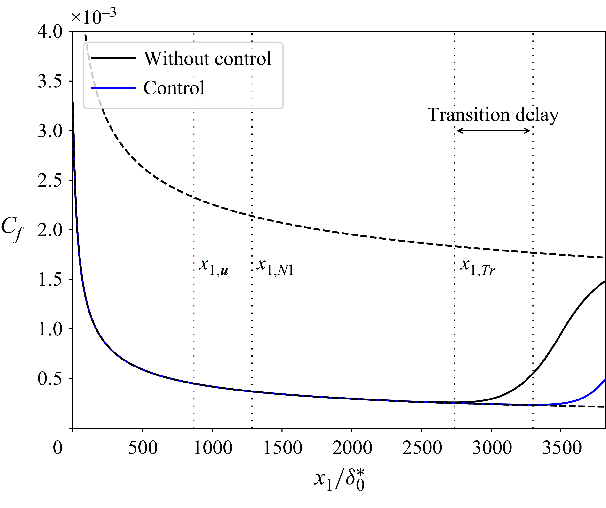
 Cf
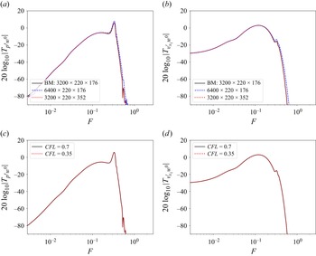
 w0
 x3=0
 x1=868.5δ0∗
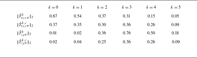
 k
 ‖Tz4w‖2
 ‖Tz1:3w‖2
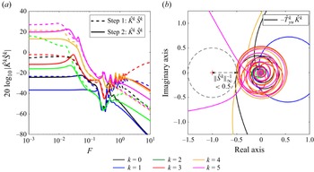
 K^kS^k
 −T^yukK^k
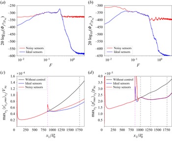
 y
 y0
 u0
 maxx2x3
 maxx2x3
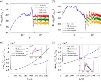
 y
 y0
 u0
 maxx2x3
 maxx2x3
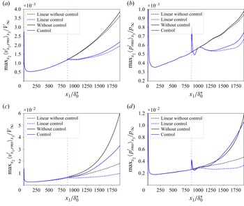
 Var[wi]=1
 Var[wi]=25
 maxx2x3
 maxx2x3
 Var[wi]/Var[wlineari]

 Open access

