

1. Introduction
The Covid-19 pandemic poses serious challenges to the macroeconomic forecaster using time series methods. The extreme values of many macroeconomic variables which occurred in the pandemic raise questions about the validity of standard time series models. For instance, will a model estimated using data from more economically stable times be appropriate for forecasting in pandemic times? When a pandemic observation on a predictor occurs which is far beyond the range of values observed in past data, is it valid to extrapolate forecasts beyond this range? Will the extreme observations occurring in the pandemic contaminate parameter estimates in our time series models, leading to poor forecast performance now and in the future? These are the questions which motivate the present paper. In it, we investigate how a particular econometric model, the mixed-frequency vector autoregression (MF-VAR) of Koop et al. (Reference Koop, McIntyre, Mitchell and Poon2020; hereafter KMMP) which is used to produce reconciled estimates of U.S. gross domestic product (GDP) growth, performs during the pandemic and whether it can be improved.
The goal of the MF-VAR of KMMP was to produce historical estimates and nowcasts of real GDP in the United States at the monthly frequency using quarterly data on two estimates of GDP produced by the Bureau of Economic Analysis (BEA). These two estimates come from measuring GDP using the expenditure and income approaches, delivering what we call GDP
E
and GDP
I
estimates.Footnote
1 Theoretically,
 $ {GDP}_E $
and
 $ {GDP}_I $
should be the same as one another. In practice, they can diverge substantially due to measurement error. This divergence can have an impact on macroeconomic forecasting and policy analysis (see, e.g., Nalewaik, Reference Nalewaik2010, Reference Nalewaik2012). This has led to the development of several econometric models for reconciling the
 $ {GDP}_E $
and
 $ {GDP}_I $
numbers so as to produce an estimate of underlying ‘true’, but latent, GDP. The reconciliation model of Aruoba et al. (Reference Aruoba, Diebold, Nalewaik, Schorfheide and Song2016) is an influential one which is used to produce the Federal Reserve Bank of Philadelphia’s popular reconciled quarterly measure of true real GDP: GDPplus.Footnote
2 The MF-VAR of KMMP builds the structure of Aruoba et al. (Reference Aruoba, Diebold, Nalewaik, Schorfheide and Song2016) into an MF-VAR involving many monthly predictors so as to successfully produce reconciled estimates of true GDP at the monthly frequency.
In this paper, we investigate how the MF-VAR of KMMP nowcasts during the pandemic in real-time and consider many extensions of it which may be better at modelling the extreme observations on many variables in 2020. These extensions involve various ways of modelling the error distribution. The model of KMMP assumed these errors to be Normal and homoskedastic. We consider several extensions which relax these two assumptions. The former is relaxed through consideration of models with fat-tailed error distributions and distributions which explicitly model outliers. The latter is relaxed by allowing for the errors to have stochastic volatility (SV). We present nowcasts of all models in a real-time nowcasting exercise for the pandemic months. We then repeat the analysis using a nowcasting method where all models’ parameters are estimated using data through 2019, and nowcasting is then done throughout 2020 where nowcasts are updated as new data releases occur each month, but the parameter estimates are not updated.
Remember that the general pattern of U.S. economic growth in 2020 was that it was slightly negative in the first quarter, very negative in the second and very positive in the third as the economy began to rebound. We compare our different nowcasting approaches in terms of how quickly and how accurately their nowcasts captured this pattern. In terms of point forecasts, we find that the original model of KMMP nowcasts at least as well as other approaches. But the other approaches often led to larger predictive variances which may be an accurate reflection of the great uncertainty in the pandemic months.
2. The MF-VAR of KMMP
The MF-VAR of KMMP builds the measurement error perspective of Aruoba et al. (Reference Aruoba, Diebold, Nalewaik, Schorfheide and Song2016) into a mixed-frequency model so as to produce monthly estimates of true GDP.Footnote
3
 $ {GDP}_E $
and
 $ {GDP}_I $
provide a great deal of information about what true GDP is at the quarterly frequency, but provide no information about how it fluctuates within the quarter. Accordingly, KMMP include many additional monthly predictors so as to increase the amount of monthly information available to pin down the month-by-month movements in true GDP.
A monthly quarterly MF-VAR can be written as follows:
 $$ {Ay}_t={By}_{t-1}+{\varepsilon}_t,{\varepsilon}_t\sim N\left(0,\Sigma \right), $$
where
 $ t=1,\dots, T $
is the time at the monthly frequency and
 $ {y}_t $
is a vector of dependent variables. Some of the variables are only observed at the quarterly frequency and, for these, they appear in
 $ {y}_t $
as unobserved monthly values.
 $ A $
is lower triangular and
 $ \Sigma $
is diagonal.Footnote
4 The MF-VAR is a state-space model where the unobserved monthly values of the quarterly variables are treated as latent states. The state-space model is completed by including measurement equations which link the unobserved monthly variables to their quarterly counterparts (i.e., imposing restrictions which reflect the fact that GDP for the 3 months in a quarter will sum to the quarterly quantity).
The main model of Aruoba et al. (Reference Aruoba, Diebold, Nalewaik, Schorfheide and Song2016) involves a vector of dependent variables
 $ {y}_t=\Big({U}_t, $
 $ {GDP}_t,{GDP}_{Et},{GDP}_{It}\Big){}^{\prime } $
, where
 $ {U}_t $
is the quarterly unemployment rate which is used as an instrument to identify the model.Footnote
5 One of the models in KMMP uses this same vector of dependent variables, except at the monthly frequency. Since
 $ {GDP}_t $
,
 $ {GDP}_{Et} $
and
 $ {GDP}_{It} $
are not observed at the monthly frequency, they enter as latent states in the MF-VAR as in KMMP. However,
 $ {U}_t $
is observed at the monthly frequency. KMMP show that the measurement error perspective can be embedded into the MF-VAR by restricting
 $$ A=\left[\begin{array}{cccc}1& 0& 0& 0\\ {}{a}_{21}& 1& 0& 0\\ {}0& -1& 1& 0\\ {}0& {a}_{42}& -1-{a}_{42}& 1\end{array}\right] $$
and
 $$ B=\left[\begin{array}{cccc}{b}_{11}& {b}_{12}& 0& 0\\ {}{b}_{21}& {b}_{22}& 0& 0\\ {}0& 0& 0& 0\\ {}0& 0& 0& 0\end{array}\right]. $$
This is the basic structure of the model of KMMP. KMMP’s empirical work (and the empirical work in the present paper) also includes additional monthly variables in the MF-VAR. But since they simply enter the model in the same manner as
 $ {U}_t $
, we will not include them to keep the notation simple.
The MF-VAR is a state-space model and standard econometric methods exist for estimation and prediction. Bayesian inference and prediction in the MF-VAR can be done by choosing a prior and using Markov chain Monte Carlo (MCMC) methods. These are described in KMMP.
3. Extensions of KMMP for pandemic nowcasting
Several attempts have been made to extend homoskedastic MF-VARs and vector autoregressions (VARs) to improve their forecast performance during the pandemic. In this section, we will briefly summarise a few of the themes which occur in a few relevant papers.Footnote 6 Then, we will suggest a few extensions to the MF-VAR of KMMP inspired by these themes.
Schorfheide and Song (Reference Schorfheide and Song2020) is an update of Schorfheide and Song (Reference Schorfheide and Song2015). The latter was a pioneering MF-VAR paper that assumed homoskedastic Normal errors. The former paper found this MF-VAR to nowcast poorly during the pandemic in a real-time exercise. However, an alternative strategy worked much better. This was one where the parameters of the MF-VAR were not updated in real-time (i.e., the parameters were estimated using data through 2019 and remained at these estimates as new data were released through the months of 2020). This raised the possibility that the extreme observations which occurred in the pandemic months of 2020 were contaminating the parameter estimates leading to poor nowcast performance. We will use this strategy as one of the approaches in our empirical work and refer to it as ‘nowcasting with 2019 parameters’. That is, all our nowcasts produced using this approach will use a model estimated on data through 2019 but then the monthly nowcasts will condition on the newly released data each month through 2020.
Another recent contribution is Lenza and Primiceri (Reference Lenza and Primiceri2020). This paper uses a VAR instead of an MF-VAR. It extends the standard homoskedastic model by assuming a mixture distribution for the errors which allows the error variance to increase by a large amount when the pandemic hits. We quote one of their conclusions: ‘Our results show that the ad hoc strategy of dropping these observations may be acceptable for the purpose of parameter estimation. However, disregarding these recent data is inappropriate for forecasting the future evolution of the economy, because it vastly underestimates uncertainty’. This quotation highlights two themes which we will investigate in our empirical work: (i) that incorporating extreme pandemic observations could have a negative impact on parameter estimates and (ii) that it may be reasonable for nowcasts to exhibit large predictive variances due to the great uncertainty that the pandemic has caused.
Several other recent contributions have developed models which allow for the pandemic to be considered an outlier or large variance shock. The treatment of the error variance is a key component in papers such as Antolin-Diaz et al. (Reference Antolin-Diaz, Drechsel and Petrella2020) and Carriero et al. (Reference Carriero, Clark, Marcellino and Mertens2020b). However, the treatment of the error variance differs between the two papers. In the former paper, it follows a mixture distribution, whereas in the latter, SV is key. But these papers share the idea that the model must allow for the error variance to increase during the pandemic period to downplay the effect of outlier observations. The idea that the pandemic period is somehow an outlier also appears in the nonparametric MF-VAR approach of Huber et al. (Reference Huber, Koop, Onorante, Pfarrhofer and Schreiner2020).
These considerations motivate our adding a variety of extensions to the model of KMMP. In relation to the error distribution, a class of different specifications can be obtained if we relax the assumption that the errors in the ith equation of the MF-VAR,
 $ {\varepsilon}_{i,t} $
, are homoskedastic and replace them with the assumption that
 $$ {\varepsilon}_{i,t}\sim N\left(0,{\lambda}_{i,t}{e}^{h_{i,t}}\right). $$
Different assumptions about
 $ {\lambda}_{i,t} $
and
 $ {h}_{i,t} $
define a wide range of different error distributions (see, e.g., Chan and Hsiao, Reference Chan, Hsiao, Jeliazkov and Yang2014).
A conventional SV model is obtained if we assume
 $ {\lambda}_{i,t}=1 $
and
 $$ {h}_{i,t}={h}_{i,t-1}+{v}_{i,t},{v}_{i,t}\sim N\left(0,{\sigma}_{h_{i,t}}^2\right). $$
If we assume
 $ {h}_{i,t} $
to be constant but
 $$ {\lambda}_{i,t}\mid {\nu}_i\sim IG\left({\nu}_i/2,{\nu}_i/2\right), $$
then the errors have a Student-t distribution with
 $ {\nu}_i $
degrees of freedom, thus allowing for heavier tails than the Normal. We refer to models involving this assumption as fat-tailed.
If we assume
 $ {h}_{i,t} $
to be constant but
 $$ \left\{\begin{array}{c}{\lambda}_{i,t}\sim U\left(2,10\right)\;\mathrm{with}\ \mathrm{probability}\ \mathrm{of}\\ {}{\lambda}_{i,t}=1\;\mathrm{with}\ \mathrm{probability}\ \mathrm{of}\end{array}\hskip0.5em \begin{array}{c}p\\ {}1-p\end{array}\right. $$
then we have a specification of the form used in Stock and Watson (Reference Stock and Watson2016), which allows for outliers. We refer to this specification as an ‘outlier model’.
Furthermore, we can add SV to the fat-tailed model or outlier model obtaining models that allow for both extreme errors and serial dependence in the volatility process.
In summary, we have two treatments of serial dependence in the volatility process (i.e., homoskedasticity and SV) and three types of distribution for the errors (i.e., Normal, fat-tailed and outlier). Considering every combination of these leads to six different models. These models range from the original model of KMMP (homoskedasticity and Normal errors) through a conventional SV specification (SV plus Normal errors) similar to Carriero et al. (Reference Carriero, Clark, Marcellino and Mertens2020b) through outlier specifications such as that used by Lenza and Primiceri (Reference Lenza and Primiceri2020) through the SV plus outlier error specification (SVO) of Stock and Watson (Reference Stock and Watson2016) and the fat-tailed plus SV specification of Antolin-Diaz et al. (Reference Antolin-Diaz, Drechsel and Petrella2020). We consider all six combinations in our empirical work.
For each of these six specifications, we carry out our nowcasting exercise in two ways. The first is a standard real-time exercise where the models are estimated on an expanding window of data and parameter estimates are updated to reflect new data releases. The second is our nowcasting with 2019 parameters strategy, where all model parameters are estimated using data through the end of 2019. Throughout the months of 2020, the nowcasts are updated to reflect new data releases, but the parameter estimates are not updated.
Details of all these models and the Bayesian methods we use for estimating and nowcasting with them are given in the Technical Appendix.
4. The data
The data were obtained from the Federal Reserve Bank of St. Louis’ FRED-MD and ALFRED databases. Our quarterly variables are
 $ {GDP}_E $
and
 $ {GDP}_I $
. Our monthly variables include unemployment, hours worked, the consumer price index, the industrial production index, personal consumption expenditure, the Federal Funds rate, the 10-year Treasury bond yield and the S&P 500 index. These variables can be expected to have predictive ability for GDP and are precisely the ones used in Schorfheide and Song (Reference Schorfheide and Song2015).Footnote
7
Aruoba et al. (Reference Aruoba, Diebold, Nalewaik, Schorfheide and Song2016) argue that measurement errors are best modelled as i.i.d. in growth rates rather than in levels and, in this paper, we follow this practice. With the exceptions of the unemployment rate, the Federal Fund rate and Treasury bond yield, all variables are log differenced. The unemployment rate is logged and the Federal Funds rate and bond yield variables are untransformed.
Our data run from 1960q1/1960m1 through November 2020. In November 2020, data through 2020Q3 were available for
 $ {GDP}_E $
, but we only had data through 2020Q2 for
 $ {GDP}_I $
. For the monthly variables, we had data through October. Our empirical work is all done in real-time and respects the release calendar. So, for instance, nowcasts made at the end of May 2020 use the vintage of data available at that time.
5. How does the MF-VAR of KMMP deal with pandemic observations?
5.1. Design of the nowcasting exercise
The MF-VAR of KMMP was found to produce reliable historical estimates and nowcasts of monthly GDP through 2019. But the question arises as to whether it will continue to do so during the pandemic. To address this question, we begin by carrying out a real-time nowcastingFootnote 8 exercise for 2020 comparing the Normal homoskedastic model of KMMP to its various extensions.
Evaluating nowcasts of true GDP is difficult, since there are no realised values of true GDP to compare them to. Hence, conventional metrics of nowcast performance, such as mean squared forecast errors, cannot be used. Hence, we evaluate our nowcasts in a less formal manner, considering how they react as new data releases occur and how our nowcasts relate to the realisations of
 $ {GDP}_E $
and
 $ {GDP}_I $
when these are available. To aid in interpretation, note that (at the time of writing) the current vintage annualised estimates for 2020Q1, Q2 and Q3 for the quarterly growth in
 $ {GDP}_E $
are −5.08 per cent, −37.66 per cent and 28.58 per cent. For
 $ {GDP}_I $
, the first two quarters are −2.56 per cent and −40.85 per cent, while the third quarter had not been released. Using data available near the end of 2019, all the nowcasts for 2020 were for moderately positive growth. In reality, 2020Q1 ended up having mildly negative growth, 2020Q2 saw severely negative growth and 2020Q3 saw a strong bounce back. The question we keep in mind when interpreting results is how quickly and how well a model discovered these unexpected (from the point of view of December 2019) extreme observations.
We undertake a fixed event nowcasting exercise for four events: 2020Q1,…,2020Q4. The goal is to nowcast true GDP for these four quarters. We produce up to 11 nowcasts for each of these events. Our initial nowcast uses information available near the end of December 2019 (denoted ‘Dec-19 Data Vintage’). By ‘near the end of’, we mean in the last week of the month. Specifically, we wait until the latest quarterly estimates of
 $ {GDP}_E $
and
 $ {GDP}_I $
have been published by the BEA, which is typically in this last week of the month, before producing density nowcasts based on this information and information known at this point in the month about the other variables in the MF-VAR. We then repeat the exercise on a month-by-month basis through the October 2020 Data Vintage. We produce nowcasts each month until the initial release of both
 $ {GDP}_E $
and
 $ {GDP}_I $
has occurred.
 $ {GDP}_E $
has a release delay of approximately 1 month and
 $ {GDP}_I $
a release delay of approximately 2 months. So, for instance, by the end of August, the BEA’s initial releases of
 $ {GDP}_E $
and
 $ {GDP}_I $
for 2020Q2 will both have occurred. Thus, we produce nine nowcasts of true GDP in 2020Q2, one based on data available near the end of December 2019 and one for each of the 8 months in 2020 through August.
Our model also produces nowcasts of monthly
 $ {GDP}_E $
and
 $ {GDP}_I $
. In the interests of brevity, these are not presented in this paper. Their properties are very similar to those for true GDP and are available on request from the authors.
5.2. Results of the nowcasting exercise
We present our results one quarter at a time. For each quarter, we present four tables. Each table compares results for the three different error distributions (Normal, fat tails and outlier). The four tables arise, since we have two treatments of SV (with and without) and two treatments of coefficient estimation (real-time estimation and estimation using data available at the end of 2019—‘nowcasting with 2019 parameters’) and we consider every combination of these cases. Thus, we have 12 different approaches. We illustrate the shape of the density nowcasts produced by each approach for each quarter of 2020 by extracting, and then tabulating, their first four moments.Footnote 9 We do so as data accumulate—the ‘Data Vintages’ are updated—through the months of 2020. To be clear when looking at the tables, the ‘Dec-19 Data Vintage’, for example, refers to when the density nowcast is produced: the relevant MF-VAR model is estimated using data as available in the last week of December 2019.
5.2.1. Nowcasting 2020Q1
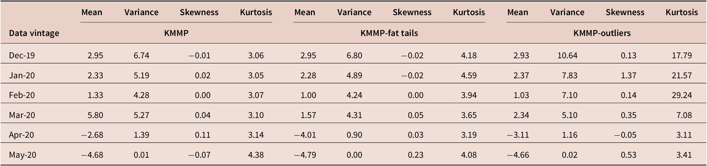
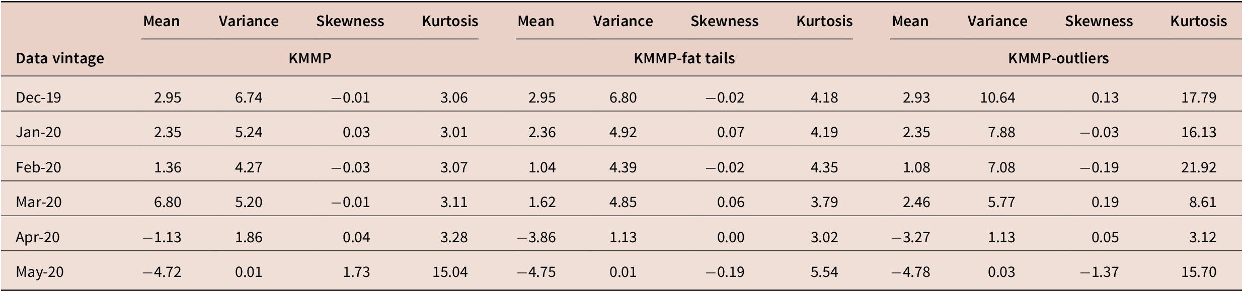
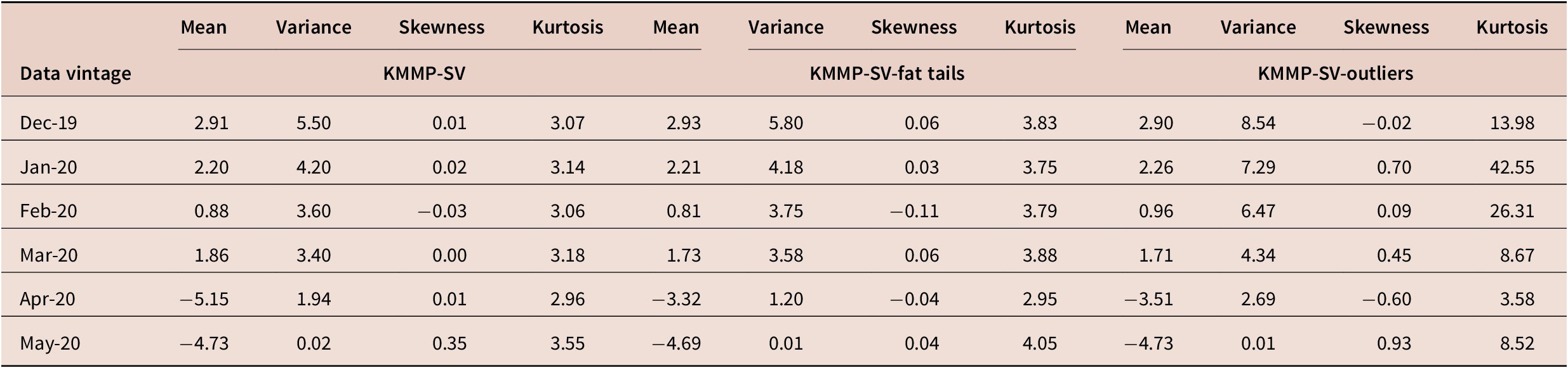
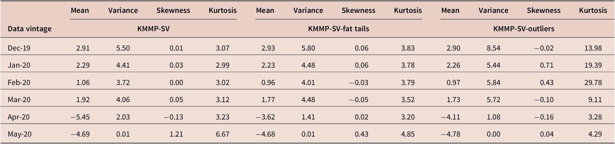
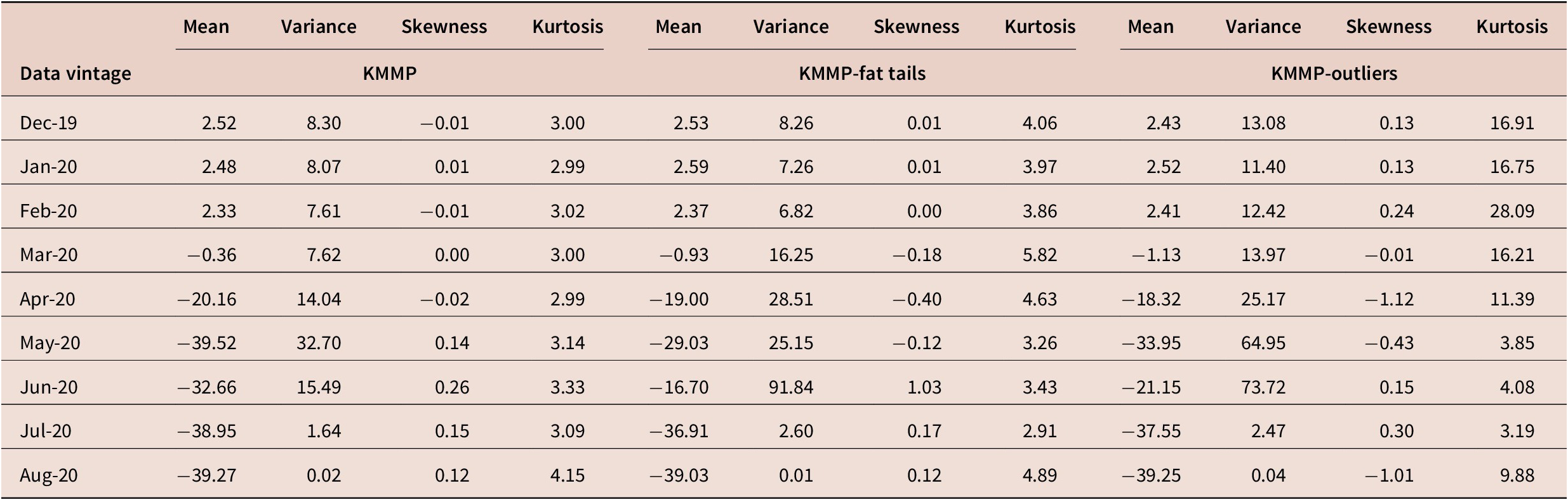
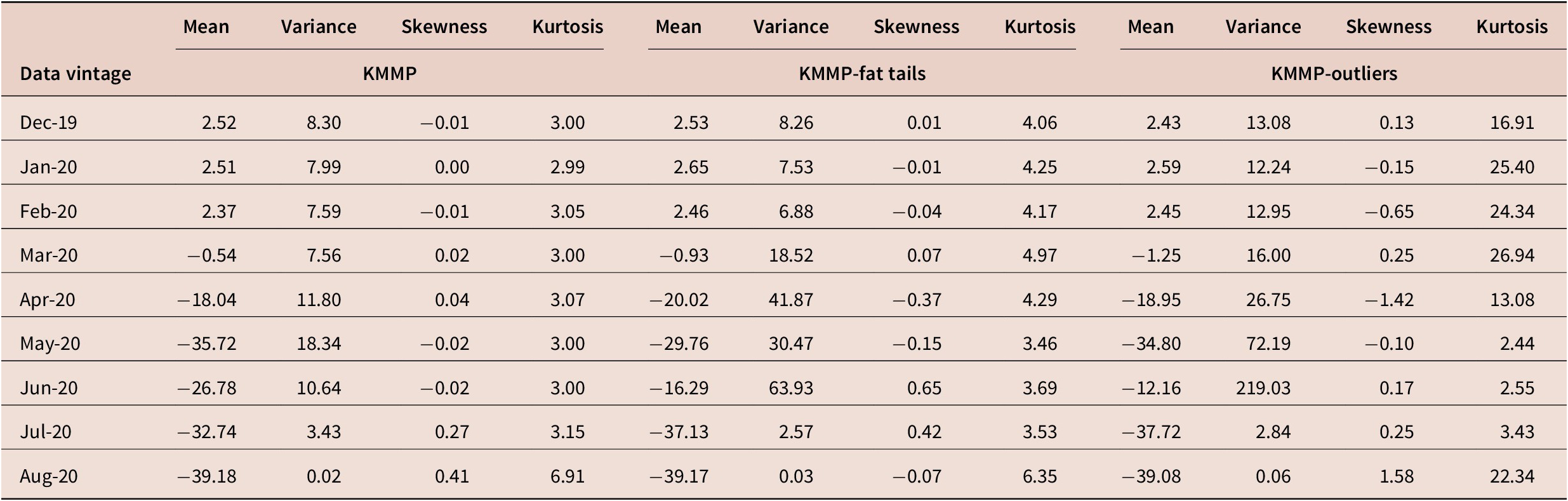
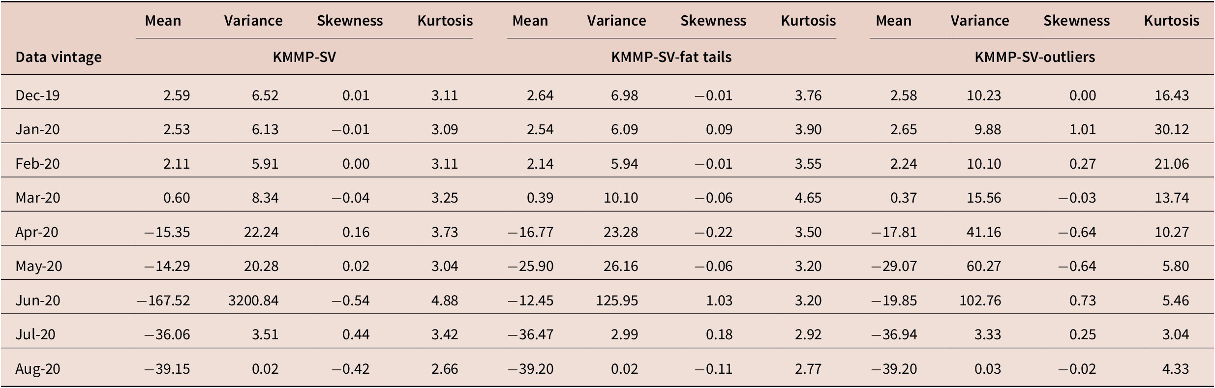
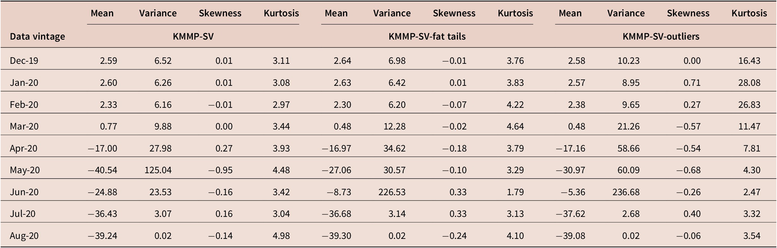
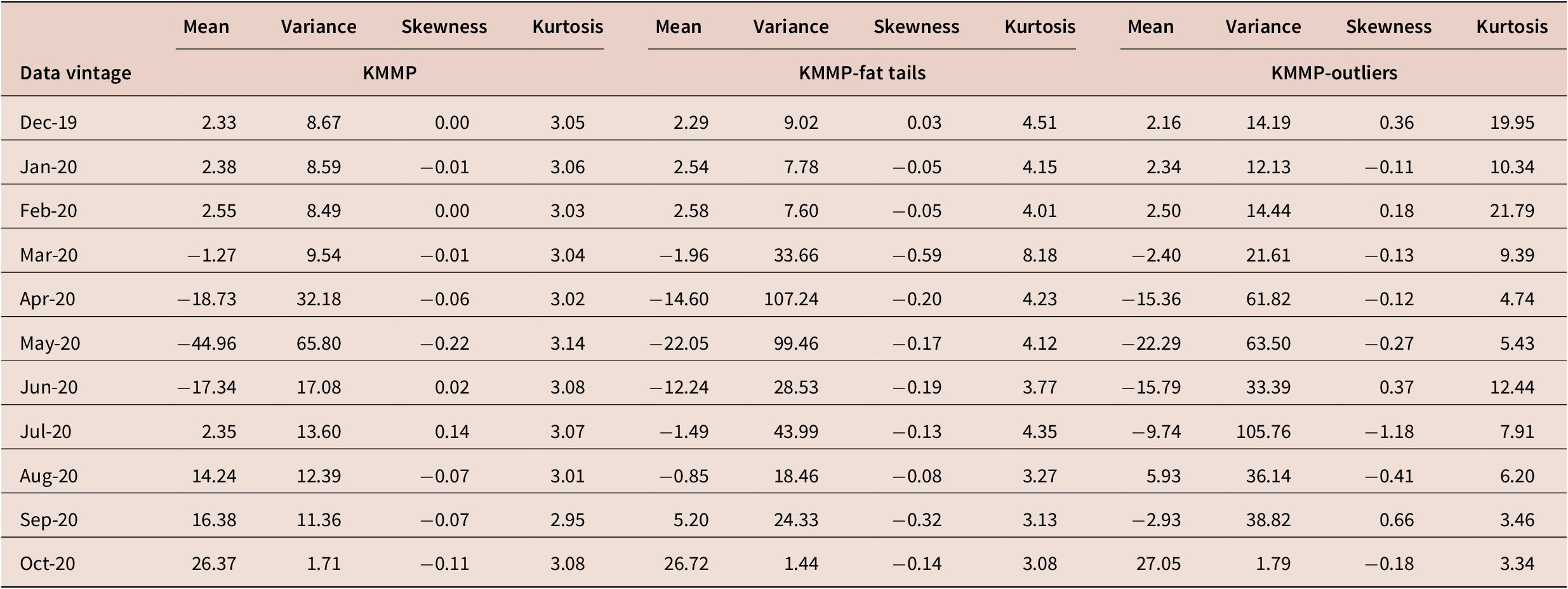
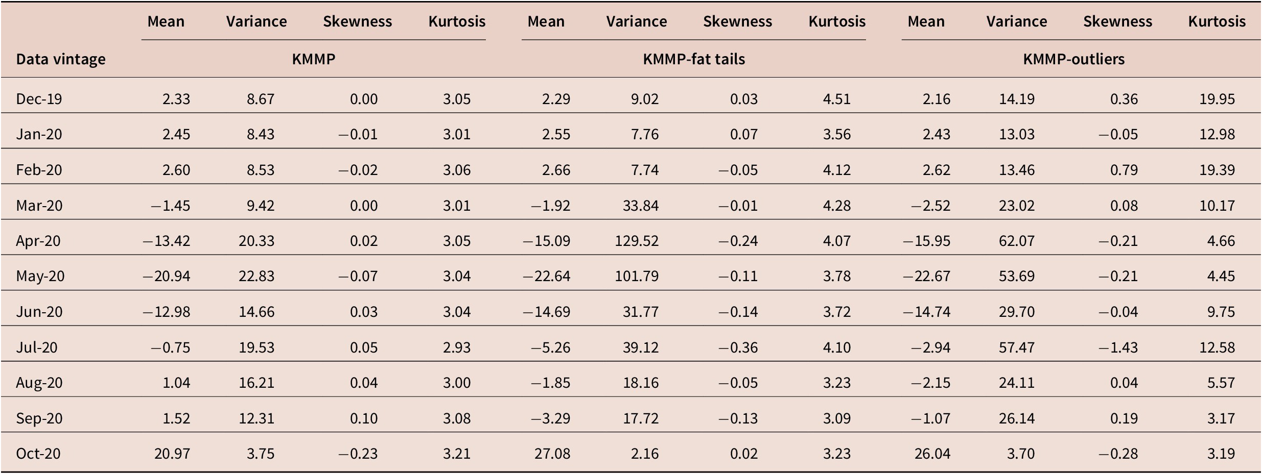
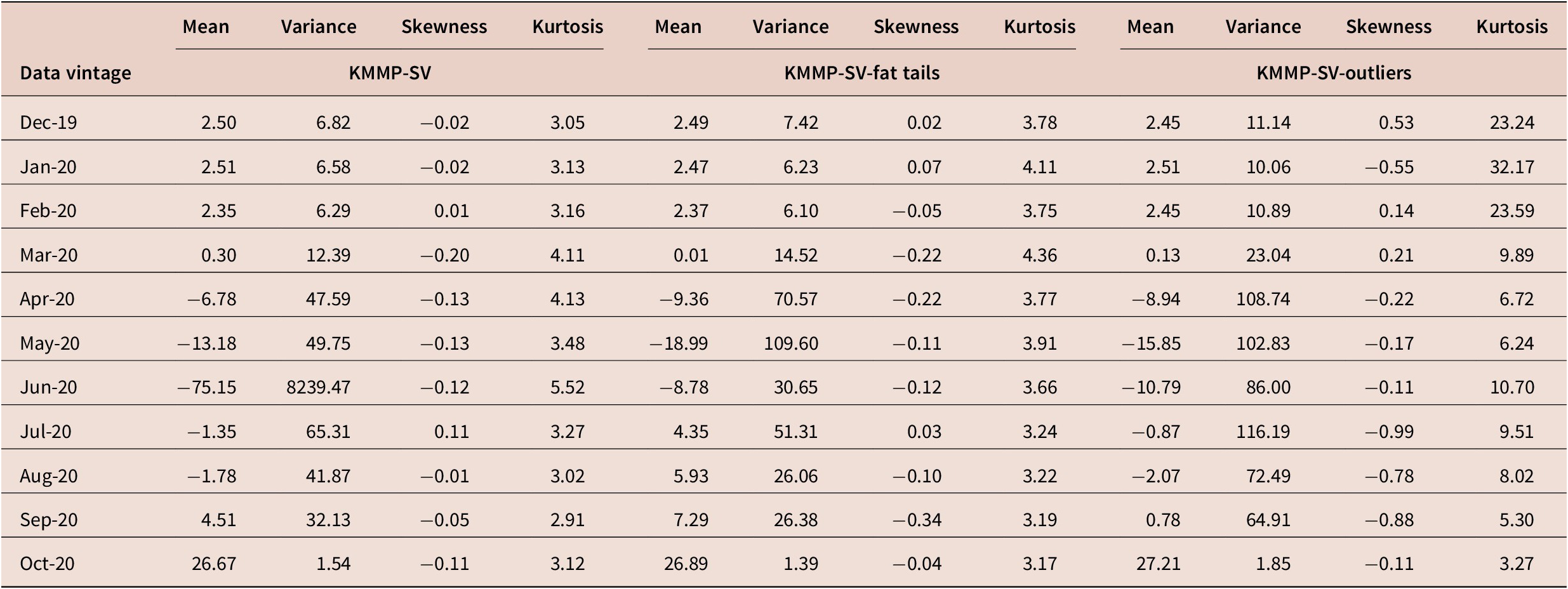
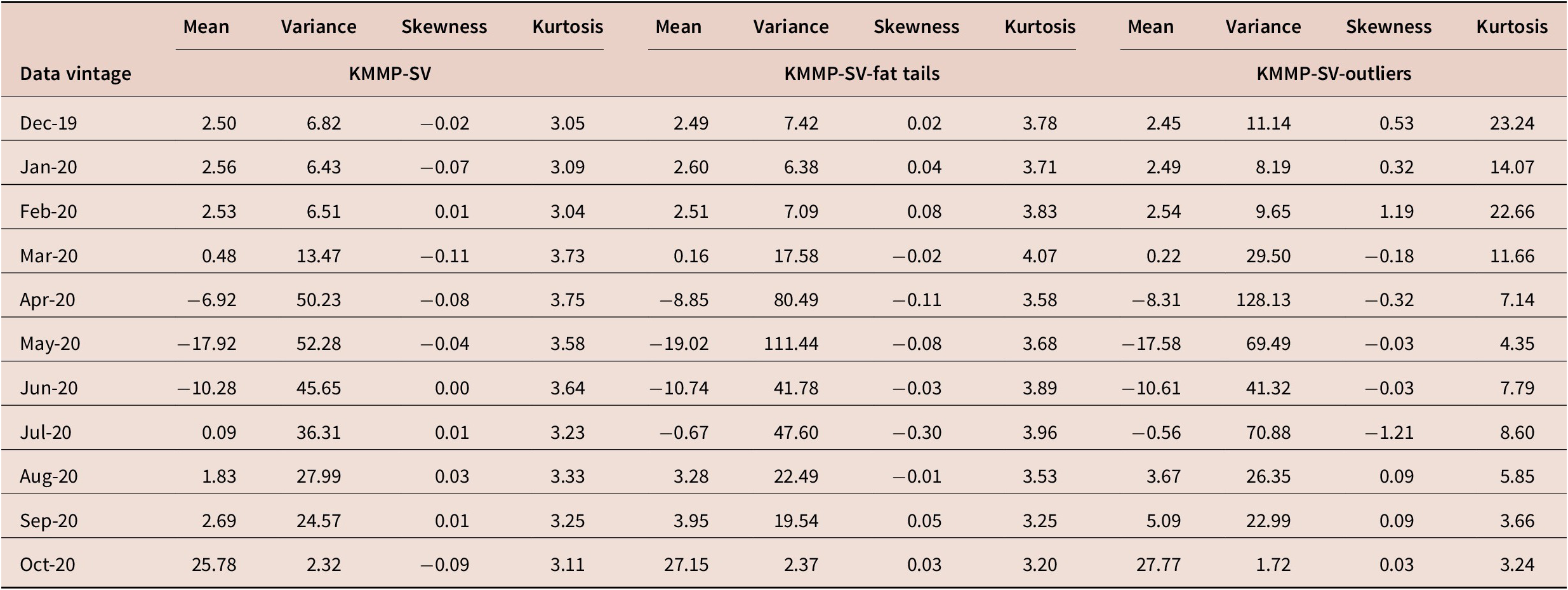
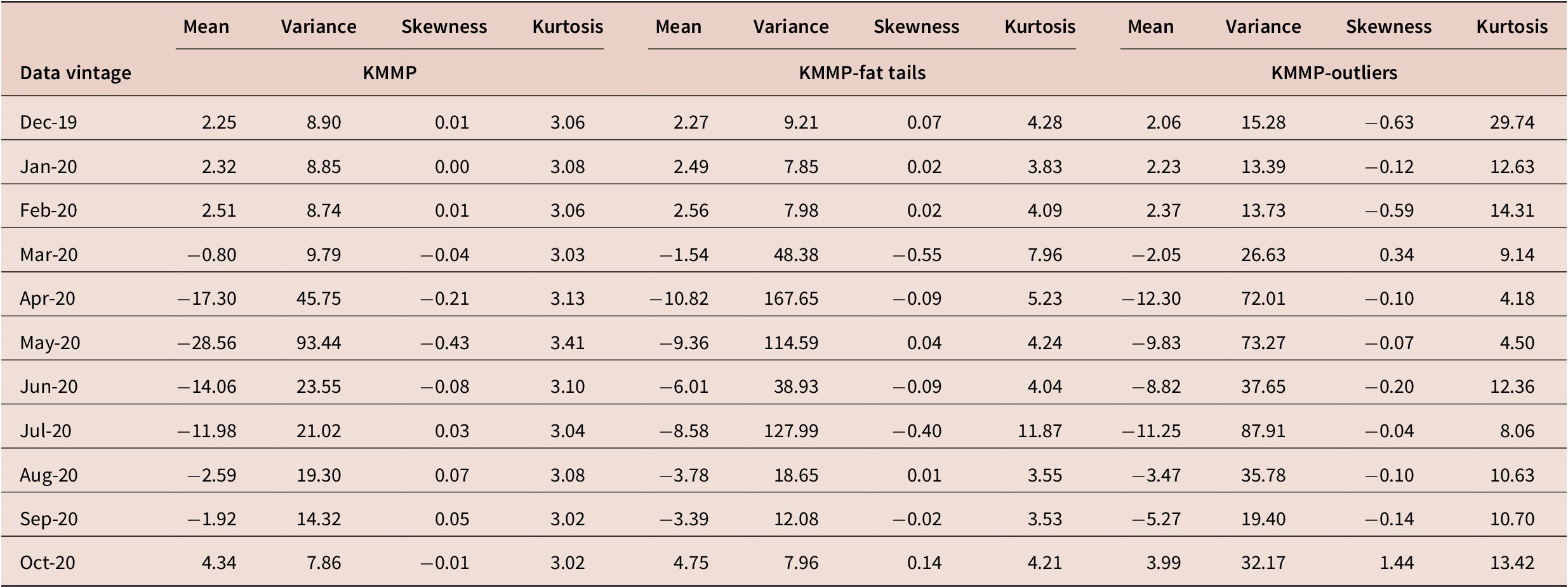
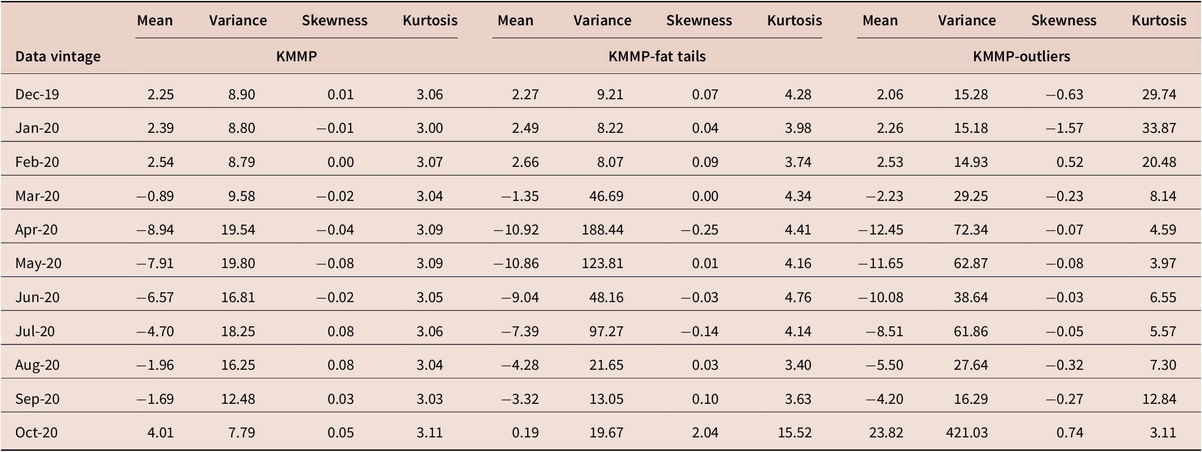
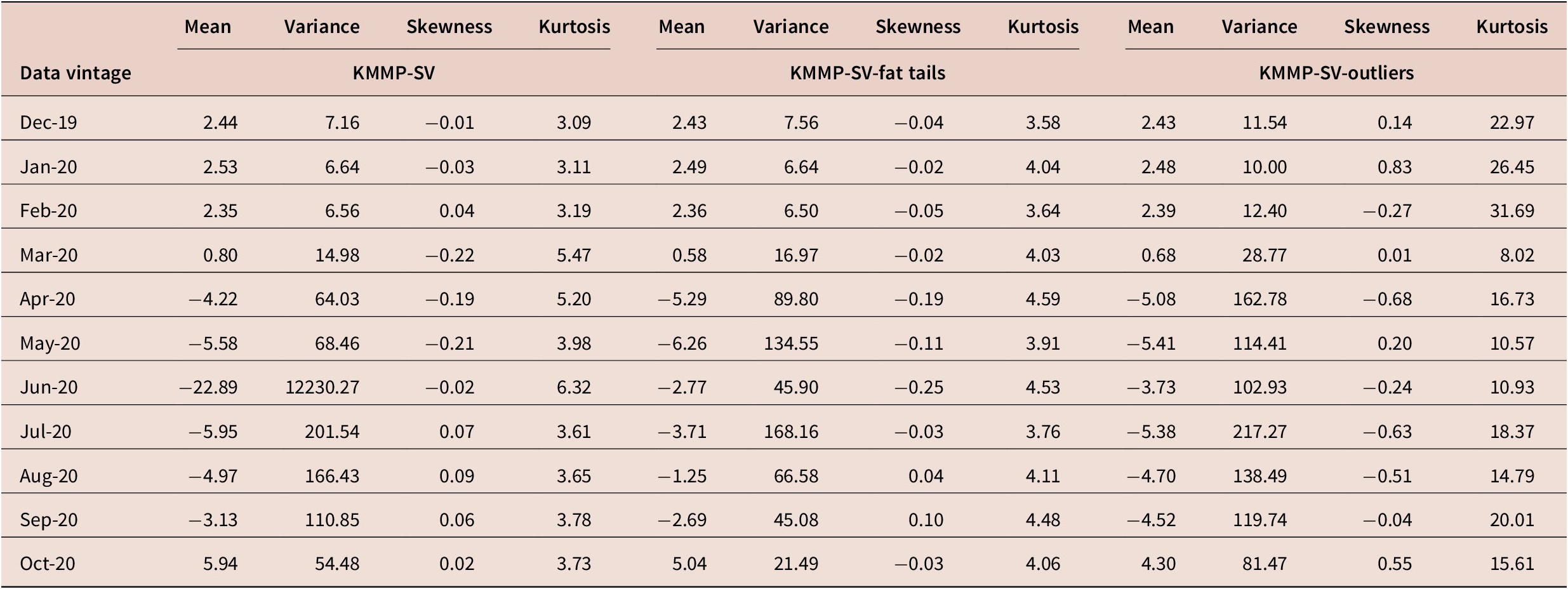
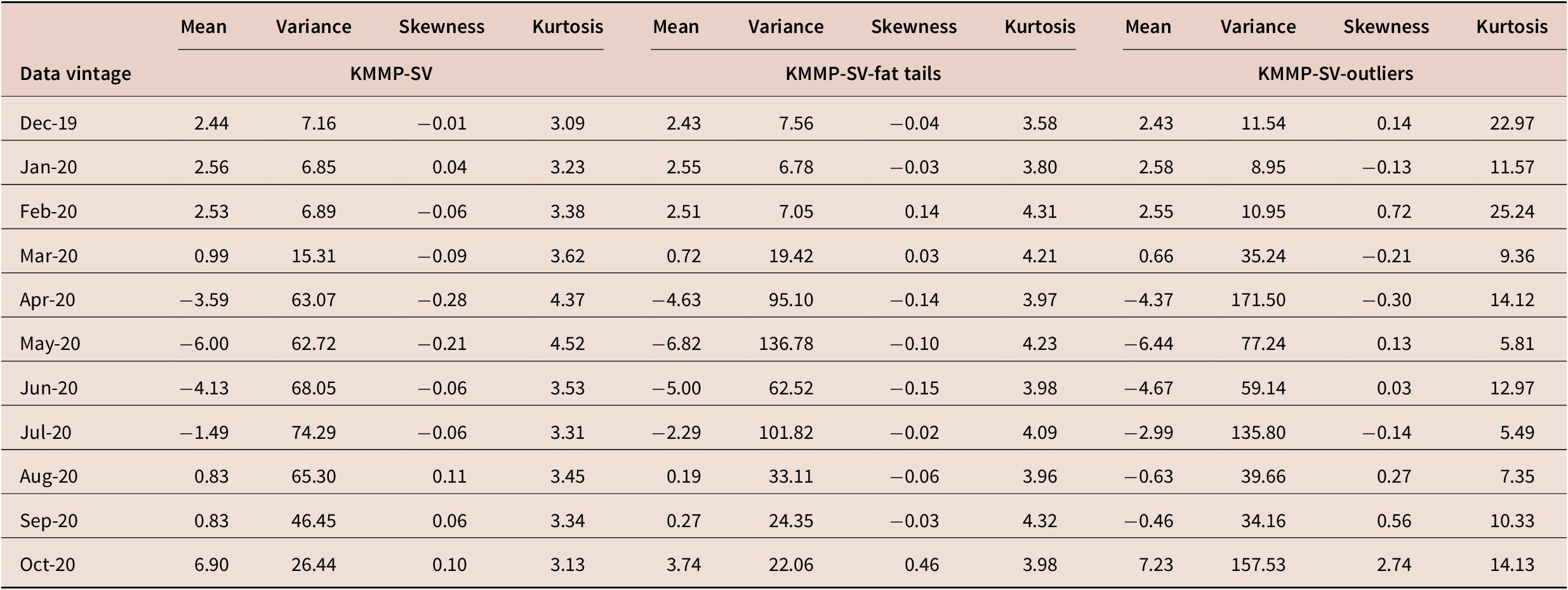
Tables 1–4 summarise the properties of our nowcast densities for 2020Q1. This quarter is of less interest than latter quarters in the pandemic, since the pandemic had little or no impact on the first 2 months of the quarter. Nevertheless, it allows us to compare our various approaches in times that are more normal.
Properties of true gross domestic product predictive densities for 2020Q1: models without stochastic volatility, parameters estimated in real-time

Properties of true gross domestic product predictive densities for 2020Q1: models without stochastic volatility, parameters estimated using data through 2019 (‘nowcasting with 2019 parameters’)

Properties of true gross domestic product predictive densities for 2020Q1: models include stochastic volatility (SV), parameters estimated in real-time

Properties of true gross domestic product predictive densities for 2020Q1: models include stochastic volatility (SV), parameters estimated using data through 2019 (‘nowcasting with 2019 parameters’)

Consider first the point nowcasts. These are similar across all 12 of our approaches. All are initially nowcasting slightly positive growth until April. At the end of April, the initial release of
 $ {GDP}_E $
, of roughly −5 per cent, occurs and the nowcasts of true GDP immediately drop to be near this value. We posit that this is due to the measurement error perspective built into all our models. That is, all models have an equation which says true GDP is
 $ {GDP}_E $
plus error which binds true GDP closely with
 $ {GDP}_E $
(and
 $ {GDP}_I $
).
Turning to higher-order predictive moments, these also tend to be quite similar across our 12 approaches. When working with these largely prepandemic datasets, the risk of parameter estimation being contaminated with outliers is very low, and results are basically the same regardless of whether estimation is done in real-time or using 2019 data. Similarly, the inclusion or not of SV has little impact. The only notable difference across approaches is that the KMMP-outliers (i.e., SVO) model tends to produce nowcasts with larger kurtosis (and slightly higher predictive standard deviations and skewness) than any of the other models.
5.2.2. Nowcasting 2020Q2
The second quarter of 2020 was the worst for the economy, as the severe lockdowns produced record breaking falls in economic output. Both
 $ {GDP}_E $
and
 $ {GDP}_I $
eventually signalled drops of around 40 per cent in this quarter. Tables 5–8 allow us to assess how quickly and accurately our different approaches to nowcasting reacted to this.
Properties of true gross domestic product predictive densities for 2020Q2: models without stochastic volatility, parameters estimated in real-time

Properties of true gross domestic product predictive densities for 2020Q2: models without stochastic volatility, parameters estimated using data through 2019 (‘nowcasting with 2019 parameters’)

Properties of true gross domestic product predictive densities for 2020Q2: models include stochastic volatility (SV), parameters estimated in real-time

Properties of true gross domestic product predictive densities for 2020Q2: models include stochastic volatility (SV), parameters estimated using data through 2019 (‘nowcasting with 2019 parameters’)

Consider first the results of the model of KMMP in table 5. In the first few, prepandemic, months of the year, the model was nowcasting positive growth. In March, the nowcast is revised down to being slightly negative (−0.36 per cent). By the end of March, the financial variables such as the stock price were signalling problems for the economy, but the macroeconomic variables such as the unemployment rate and industrial production were not yet signalling problems, due to their backward-looking nature and release delays. By the end of April (with the initial release of
 $ {GDP}_E $
for 2020Q1, as well as poor monthly values for many of the monthly variables being released), the model of KMMP is producing a point nowcast of strong negative growth of −20 per cent. But it is only by the May data vintage and subsequent months that the point nowcasts move to the region of −40 per cent, which is close to the eventual realisations of
 $ {GDP}_E $
and
 $ {GDP}_I $
. May is an important month, since this is when a particularly extreme observation occurs: the unemployment rate went up by 250 per cent in April. This information was released in May and hence forms part of the May 2020 data vintage. The model of KMMP captured this negative signal well and lowered its point nowcast to extremely negative GDP growth.
The preceding paragraph discussed the point nowcasts. The predictive variances are quite large in May and June and only become small at the end of July when the initial release of 2020Q2
 $ {GDP}_E $
occurs. We would argue this is sensible and illustrates a pattern found throughout our results. The model of KMMP is reacting well to the information in the monthly variables in terms of the point nowcasts. But information signalled in them is not sufficient to reduce the great uncertainty in pandemic times, and this is reflected in large predictive variances. It is only when information on one of the GDP proxies is released that the uncertainty in the nowcasts is vastly reduced. This reflects the measurement error perspective embedded in this model which links contemporaneous values of true GDP to
 $ {GDP}_E $
and
 $ {GDP}_I $
.
We next discuss whether any of the other approaches does better than the model of KMMP. Overall, our 12 different approaches tend to produce similar nowcasts. But there are a few places where they differ somewhat and it is these differences we will discuss here. If we focus on the crucial months of April, May and June, then a pattern (with some exceptions) is that adding SV, fat-tails or a mixture distribution tends to lead to larger predictive variances and often larger kurtosis (but only rarely are we finding evidence of skewness and where we do it is associated with the outlier model). As one example, consider the June 2020 nowcasts from the fat-tailed model in table 5. The point nowcast −16.70 per cent is substantially worse than the −32.66 per cent point nowcast of the KMMP model when considered against the realisations of 2020Q2
 $ {GDP}_E $
and
 $ {GDP}_I $
. However, the fat-tailed model is producing a predictive variance which is over six times as large as that produced by KMMP. A similar pattern is observed with the outlier model. Adding SV also tends to lead to much larger predictive variances, particularly in months such as June.
June 2020 is an interesting month, since by the end of this month, it is known that: the 2020Q1 outcomes of
 $ {GDP}_E $
and
 $ {GDP}_I $
were slightly negative, many of the monthly variables for April were signalling extremely bad outcomes, but some of the monthly variables were recovering in May from the new lows set in April. In the face of these conflicting signals, models with non-Normal errors and/or SV tended to be highly uncertain in the nowcasts they produce and this is reflected in large predictive standard deviations in key months. Possibly, this is an accurate reflection of the great uncertainty of those pandemic months and, thus, one can argue that these extensions of KMMP are warranted. However, it is the case that for 2020Q2 KMMP produced predictive densities that more quickly allocated more weight to the extreme negative economic growth which actually occurred in 2020Q2.
5.2.3. Nowcasting 2020Q3
The third quarter of 2020 saw
 $ {GDP}_E $
and
 $ {GDP}_I $
partially bounce back after the collapse of 2020Q2. Tables 9–12 reveal a consistent pattern for all our 12 models. In April, May and June, all models were missing the bounce back and still nowcasting negative growth for 2020Q3, but subsequently, the nowcasts turn positive until by the end of October (when the initial release of
 $ {GDP}_E $
for 2020Q3 of almost 30 per cent growth arrived) strong positive growth was nowcast.
Properties of true gross domestic product predictive densities for 2020Q3: models without stochastic volatility, parameters estimated in real-time

Properties of true gross domestic product predictive densities for 2020Q3: models without stochastic volatility, parameters estimated using data through 2019 (‘nowcasting with 2019 parameters’)

Properties of true gross domestic product predictive densities for 2020Q3: models include stochastic volatility (SV), parameters estimated in real-time

Properties of true gross domestic product predictive densities for 2020Q3: models include stochastic volatility (SV), parameters estimated using data through 2019 (‘nowcasting with 2019 parameters’)

But within this general pattern, there are some differences between the various approaches. Consider the point forecasts which, with the exception of the basic KMMP model, all show nowcasts of 2020Q3 growth in single digits until the end of October. In contrast, the homoskedastic model of KMMP was nowcasting 14 per cent growth by the end of August. Its point nowcasts identified the upturn faster than the other models. As for the 2020Q2 results, we are finding that the alternative models which add SV and fat-tails, or accommodate outliers, tend to produce predictive variances which are larger than the homoskedastic model of KMMP. This increase in uncertainty could be taken as a desirable property in the context of the information available in the summer of 2020. Until the end of October, the information available to the models was the fact that
 $ {GDP}_E $
and
 $ {GDP}_I $
had collapsed in 2020Q2 plus information in the monthly variables. The former was a bad signal and the latter a good signal for the economy in Q3. In the face of such conflicting signals, it would be difficult for any time series econometric model to nowcast strong growth in 2020Q3. But KMMP is placing more weight on the good information in the monthly variables in August and September. This could be because the other approaches allow for outliers and/or increases in the error variances. These tend to downplay the information in outliers; so, when strong positive news was arriving via the monthly predictors in August and September, this tended to be given less weight by the other approaches. Thus, a property of Normal homoskedastic models that is often considered bad (i.e., that they are not robust to outliers) actually benefited the KMMP model in that it did not downplay the good news of August and September.
The other key difference between the Normal homoskedastic KMMP model and all the extensions we are considering is the one noted in our discussion of the 2020Q2 results. The extensions typically lead to greater uncertainty reflected in larger predictive variances. As one example of this, compare the predictive variances of the Normal homoskedastic version of KMMP with a model which is the same except that it allows for SV (i.e., compare the KMMP results in table 9 to the KMMP-SV results in table 11). Predictive variances in the latter are much larger than the former.
5.2.4. Nowcasting 2020Q4
As of the time of writing, neither
 $ {GDP}_E $
nor
 $ {GDP}_I $
for 2020Q4 has been released. Tables 13–16 show how our nowcasts of these have evolved over the year as new information on the pandemic’s impact on the economy became available each month. Using data through the end of October, all of our models are nowcasting positive growth for 2020Q4, but they differ substantially in how certain they are about this. That is, predictive variances differ a lot across specifications and in the same way as noted in our discussion of the nowcasts of earlier quarters. The extensions of the Normal homoskedastic model of KMMP all tend to produce larger predictive variances than the original model did. These larger predictive variances are particularly notable in models with SV or which use mixture of distributions to model outliers, but are less noticeable for the fat-tails model.
Properties of true gross domestic product predictive densities for 2020Q4: models without stochastic volatility, parameters estimated in real-time

Properties of true gross domestic product predictive densities for 2020Q4: models without stochastic volatility, parameters estimated using data through 2019 (‘nowcasting with 2019 parameters’)

Properties of true gross domestic product predictive densities for 2020Q4: models include stochastic volatility (SV), parameters estimated in real-time

Properties of true gross domestic product predictive densities for 2020Q4: models include stochastic volatility (SV), parameters estimated using data through 2019 (‘nowcasting with 2019 parameters’)

Finally, we have not offered much discussion of the comparison between models which estimate the parameters in real-time and those which estimate them using data through 2019 (i.e., using the nowcasting with 2019 parameters strategy). In contrast to what some other researchers have found, we have not found a great difference in their nowcasting densities. We posit that this is because of the measurement error perspective built into our MF-VARs. That is, all of our models include equations which impose the restriction that, with an error, true GDP equals one of its proxies. The parameters in such equations are not estimated (other than their error variances) and, thus, are not liable to be contaminated by outliers. Although outliers potentially contaminate the estimates of the coefficients in the remainder of the MF-VAR (i.e., the equations for the monthly variables), this does not seem enough to negatively impact on our nowcasts.
6. Conclusions
It is always important to provide timely and high-frequency nowcasts of GDP. But, in pandemic times, it is even more important. The Normal homoskedastic MF-VAR model of Koop et al. (Reference Koop, McIntyre, Mitchell and Poon2020) was found to produce high-quality nowcasts using data through 2019. This paper addresses the question of whether it can also produce high-quality nowcasts in a time of great economic instability, and whether various extensions to the model specification improve its nowcasting performance through the pandemic.
Overall, we find that the KMMP model does a good job of doing so, reacting quickly as new information is released each month. It is especially effective at updating nowcasts in months when new releases of
 $ {GDP}_E $
and
 $ {GDP}_I $
occur. This is due to what Aruoba et al. (Reference Aruoba, Diebold, Nalewaik, Schorfheide and Song2016) call the measurement error perspective. It is built into the KMMP model and provides tight links between GDP and its two noisy proxies. But updates also occur using the information in the monthly predictors included in the model.
The various extensions of KMMP we tried in this paper, involving SV and more flexible error distributions, tend to produce similar point nowcasts to KMMP. But, in some cases, the KMMP point nowcasts react more quickly to new data releases. That is, they move towards values consistent with the eventual
 $ {GDP}_E $
and
 $ {GDP}_I $
releases earlier than those produced by alternative approaches. A property of Normal homoskedastic models that is often considered bad (i.e., that they are not robust to outliers) actually benefits the KMMP model when nowcasting, as it reacts confidently to the rapidly evolving economic data. The extensions do, in many cases, increase the predictive variances leading to more uncertainty about the nowcasts. This may not be helpful for the policymaker interested in precise information, but may be an accurate reflection of the uncertainty which occurred during pandemic times. As emphasised by Lerch et al. (Reference Lerch, Thorarinsdottir, Ravazzolo and Gneiting2017), any statistical evaluation of these density nowcasts needs to be mindful of the forecaster’s dilemma, namely that even the most skilful forecasts can be disfavoured in the presence of outliers. It is important to evaluate nowcasts and forecasts over long samples, not just over periods of extreme events, although scoring rules that emphasise specific regions of the density, such as the tails, may be useful.
Acknowledgements
Portions of this research were conducted under independent contract for the Federal Reserve Bank of Cleveland; the views expressed herein are those of the authors and not necessarily those of the Federal Reserve Bank of Cleveland or the Federal Reserve System. We would like to thank Ana Galvao, Kevin Lee, Massimiliano Marcellino, Ivan Petrella and other participants at the National Institute of Economic and Social Research workshop ‘The Impact of the Covid-19 Pandemic on Macroeconomic Forecasting’ for constructive comments on this work.
A. Technical appendix
A.1 The model of KMMP
The model of KMMP, which assumes the errors are homoskedastic and Normal, is defined in their paper, and details of the econometrics, including priors and development of an MCMC algorithm for posterior and predictive inference, are given there. The version of the model we use is called SS(N) (Schorfheide and Song, with noise restriction imposed) in KMMP.
A.2 Adding stochastic volatility
We can rewrite the model of KMMP as a set of individual equations for
 $ i=1,\dots, N $
variables as follows:
 $$ {y}_{i,t}={X}_{i,t}{\beta}_i+{\varepsilon}_{i,t}. $$
SV is present if we assume
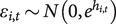 $ {\varepsilon}_{i,t}\sim N\left(0,{e}^{h_{i,t}}\right) $
with
 $$ {h}_{i,t}={h}_{i,t-1}+{v}_{i,t},{v}_{i,t}\sim N\left(0,{\sigma}_{h_{i,t}}^2\right). $$
The priors for
 $ {\beta}_i $
are the same as those in KMMP, and the reader is referred to our earlier paper for justification of our prior choice. The priors for the SV terms are:
 $ {h}_{i,0}\sim N\left(0,1\right) $
,
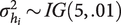 $ {\sigma}_{h_i}^2\sim IG\left(5,.01\right) $
for the errors in the equations for the monthly variables. For the
 $ {GDP}_t $
equation, the priors for parameters in the SV are
 $ {h}_{GDP,0}\sim N\left(0,1\right), $
 $ {\sigma}_{h_{GDP}}^2\sim IG\left(10,.001\right). $
We do not add SV to the errors for the equations for
 $ {GDP}_{E,t} $
and
 $ {GDP}_{I,t} $
, since these variables are latent and the latent true GDP which appears on the right-hand side of these equations already has SV in it and, thus, adding SV to the errors as well would induce two SV processes in these equations. The priors for the constant error variances in these equations are
 $ {\sigma}_{EE}^2, $
 $ {\sigma}_{II}^2\sim IG\left(5,01\right) $
.
MCMC methods involving adding a step for drawing
 $ {h}_{i,t} $
to the MCMC algorithm of KMMP. This is standard; see, for instance, Chan and Hsiao (Reference Chan, Hsiao, Jeliazkov and Yang2014).
A.3 Adding fat-tails
The KMMP model with fat-tail SV errors is
 $$ {y}_{i,t}={X}_{i,t}{\beta}_i+{\varepsilon}_{i,t},{\varepsilon}_{i,t}\sim N\left(0,{\lambda}_{i,t}{e}^{h_{i,t}}\right), $$
 $$ {\lambda}_{i,t}\mid {\nu}_i\sim IG\left({\nu}_i/2,{\nu}_i/2\right), $$
 $$ {h}_{i,t}={h}_{i,t-1}+{v}_{i,t},{v}_{i,t}\sim N\left(0,{\sigma}_{h_i}^2\right). $$
The priors for all parameters except
 $ {\nu}_i $
are the same as those specified for the KMMP model with SV. For the degrees of freedom parameter, we use a prior of
 $ {\nu}_i\sim U\left(5,50\right) $
.
MCMC methods involving adding a step for drawing
 $ {\nu}_i $
to the MCMC algorithm of the KMMP with SV model. This is standard; see, for instance, Chan and Hsiao (Reference Chan, Hsiao, Jeliazkov and Yang2014).
The version of the fat-tailed model which does not have SV is the restricted special case of this model with
 $ {h}_{i,t} $
replaced by
 $ {h}_i $
and given the same treatment as in KMMP.
A.4 Adding outliers
The model which allows for outliers and SV takes the form:
 $$ {y}_{i,t}={X}_{i,t}{\beta}_i+{\varepsilon}_{i,t},{\varepsilon}_{i,t}\sim N\left(0,{\lambda}_{i,t}^2{e}^{h_{i,t}}\right), $$
 $$ {h}_{i,t}={h}_{i,t-1}+{v}_{i,t},{v}_{i,t}\sim N\left(0,{\sigma}_{h_i}^2\right), $$
with
 $$ \left\{\begin{array}{cc}\begin{array}{c}{\lambda}_{i,t}\sim U\left(2,10\right)\;\mathrm{with}\ \mathrm{probability}\ \mathrm{of}\\ {}{\lambda}_{i,t}=1\;\mathrm{with}\ \mathrm{probability}\ \mathrm{of}\end{array}& \begin{array}{c}{p}_i\\ {}1-{p}_i\end{array}\end{array}\right.. $$
The prior for
 $ {p}_i\sim Beta\left({a}_0,{b}_0\right) $
, where
 $ {a}_0=\frac{1}{4m}10m $
,
 $ {b}_0=\left(1-\frac{1}{4m}\right)20m $
. We follow Stock and Watson (Reference Stock and Watson2016) and set
 $ m=12 $
, since we are working with monthly data. Other prior choices are the same as for the KMMP model with SV.
The MCMC algorithm involves the algorithm for the KMMP with SV model with extra steps for drawing the parameters relating to the outlier process. This is done by defining an indicator variable
 $ {S}_{it} $
, where
 $ {S}_{it}=1 $
implies a model of
 $ N\left({X}_{i,t}{\beta}_i,{\lambda}_{i,t}^2{e}^{h_{i,t}}\right) $
and
 $ {S}_{it}=0 $
implies a model of
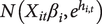 $ N\left({X}_{it}{\beta}_i,{e}^{h_{i,t}}\right) $
.
 $ {S}_{it} $
can be drawn in the MCMC algorithm from the following distribution:
 $$ \mathrm{\mathbb{P}}\left({S}_{it}=1|{y}_{it},{\beta}_i,{h}_{it}\right)=\frac{p_i\times \phi \left({y}_{it},{X}_{i,t}{\beta}_i,{\lambda}_{it}^2{e}^{h_{it}}\right)}{p_i\times \phi \left({y}_{it},{X}_{i,t}{\beta}_i,{\lambda}_{it}^2{e}^{h_{it}}\right)+\left(1-{p}_i\right)\phi \left({y}_{it},{X}_{i,t}{\beta}_i,{e}^{h_{it}}\right)}, $$
 $$ \mathrm{\mathbb{P}}\left({S}_{it}=0|{y}_{it},{\beta}_i,{h}_{it}\right)=1-\mathrm{\mathbb{P}}\left({S}_{it}=1|{y}_{it},{\beta}_i,{h}_{it}\right), $$
where
 $ \phi \left(a,\mu, {\sigma}^2\right) $
is a Normal density with a mean
 $ \mu $
and variance
 $ {\sigma}^2 $
.
When
 $ {S}_{it}=1 $
, this implies the prior for
 $ {\lambda}_{it}\sim U\left(2,10\right) $
. Then, the log conditional posterior for
 $ {\lambda}_{it} $
is
 $$ p\left({\lambda}_{it}|{y}_{it},{\beta}_i,{h}_{i,t}\right)\propto -\frac{1}{2}\mathit{\log}\left(2\pi \right)-\frac{1}{2}\mathit{\log}\left({\lambda}_{it}^2{e}^{h_{i,t}}\right)-\frac{1}{2}\frac{{\left({y}_{it}-{X}_{i,t}{\beta}_i\right)}^2}{\lambda_{it}^2{e}^{h_{it}}}, $$
where
 $ 2<{\lambda}_{it}<10 $
. To approximate this density,
 $ p\left({\lambda}_{it}|{y}_{it},{\beta}_i,{h}_{i,t}\right) $
, we use a Griddy-Gibbs sampler that bounds the support between
 $ \left[2,10\right] $
.
Lastly, the conditional posterior for
 $ {p}_i $
is
 $ {p}_i\mid \bullet \sim Beta\left({a}_0+{T}_1,{b}_0+{T}_2\right) $
, where is
 $ {T}_1 $
is the number of times in the observations
 $ {S}_t=1 $
and
 $ {T}_2=T-{T}_1 $
.
The version of the fat-tailed model which does not have SV is the restricted special case of this model with
 $ {h}_{i,t} $
replaced by
 $ {h}_i $
and given the same treatment as in KMMP.