1 Introduction
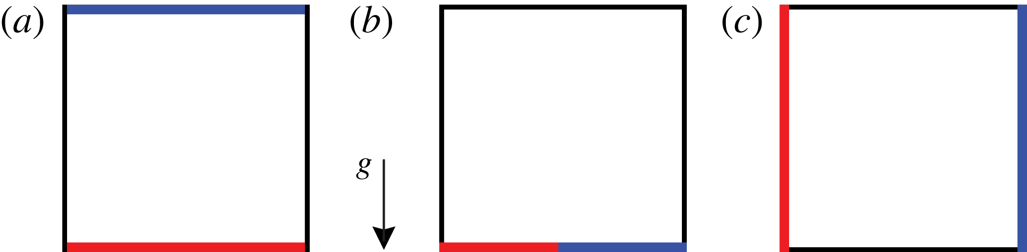
Thermally driven flows play a crucial role in nature and are associated with many engineering flows. To study such flows, researchers typically consider idealised set-ups which include (figure 1
a) the classical Rayleigh–Bénard convection, or RBC (Ahlers, Grossmann & Lohse Reference Ahlers, Grossmann and Lohse2009; Lohse & Xia Reference Lohse and Xia2010; Chillà & Schumacher Reference Chillà and Schumacher2012), where fluid is confined between a heated bottom plate and a cooled upper plate, (figure 1
b) horizontal convection, or HC (Hughes & Griffiths Reference Hughes and Griffiths2008; Shishkina, Grossmann & Lohse Reference Shishkina, Grossmann and Lohse2016), where fluid is heated at one part of the bottom plate and cooled at some other part and (figure 1
c) vertical natural convection, or VC (Ng et al.
Reference Ng, Ooi, Lohse and Chung2015, Reference Ng, Ooi, Lohse and Chung2017), where fluid is confined between two vertical walls, one heated and one cooled, i.e. the flow is driven by a horizontal average heat flux. Alternative configurations of the VC flow, such as in a confined cavity (Patterson & Armfield Reference Patterson and Armfield1990; Yu, Li & Ecke Reference Yu, Li and Ecke2007) and in a confined cylinder (Shishkina Reference Shishkina2016; Shishkina & Horn Reference Shishkina and Horn2016) have also been investigated. In all these studies on thermal convection, there is a common interest to physically understand and predict how the temperature difference imposed on the flow (characterised by the Rayleigh number
 $\mathit{Ra}$
) influences the heat flux (characterised by the Nusselt number
 $\mathit{Nu}$
) and the degree of turbulence (characterised by the Reynolds number
 $\mathit{Re}$
). With such relations, one is able to avoid relying on empirical relationships that are undetermined outside the range of calibration and which ignore the underlying physics.
Examples of wall-bounded configurations for (a) Rayleigh–Bénard convection (RBC), (b) horizontal convection (HC) and (c) vertical natural convection (VC). For illustration purposes, the configurations are drawn in a cavity with aspect ratio equal to one. Heated walls are indicated in red and cooled walls in blue.
 $g$
is the gravity vector.

At high
 $\mathit{Ra}$
, Kraichnan (Reference Kraichnan1962) and Grossmann & Lohse (Reference Grossmann and Lohse2000, Reference Grossmann and Lohse2001, Reference Grossmann and Lohse2002, Reference Grossmann and Lohse2004) – hereinafter referred to as the GL theory – predicted the so-called asymptotic ultimate-regime scaling where
 $$\begin{eqnarray}\displaystyle \mathit{Nu}\sim \mathit{Ra}^{1/2},\quad \mathit{Re}\sim \mathit{Ra}^{1/2}, & & \displaystyle\end{eqnarray}$$
for low
 $\mathit{Pr}$
-values, for instance, when
 $\mathit{Pr}\leqslant 1$
. (The
 $\mathit{Pr}$
-dependence of
 $\mathit{Nu}\sim \mathit{Pr}^{1/2}$
and
 $\mathit{Re}\sim \mathit{Pr}^{-1/2}$
predicted by the GL theory for this asymptotic ultimate regime was confirmed in Calzavarini et al. (Reference Calzavarini, Lohse, Toschi and Tripiccione2005) in the case of homogeneous RBC. For homogeneous VC, the
 $\mathit{Pr}$
-dependence is expected to be the same, but is beyond the scope of this paper.) These scaling relations contain logarithmic corrections when boundary layers or plumes are prominent (Grossmann & Lohse Reference Grossmann and Lohse2011). In numerical studies that seek to model only bulk thermal convection, i.e. without boundary layers, the
 $1/2$
-power-law scalings were indeed subsequently reported: Lohse & Toschi (Reference Lohse and Toschi2003) and Calzavarini et al. (Reference Calzavarini, Lohse, Toschi and Tripiccione2005, Reference Calzavarini, Doering, Gibbon, Lohse, Tanabe and Toschi2006a
) discounted the influence of boundary layers by simulating a triply periodic configuration for RBC, termed homogeneous RBC. Schmidt et al. (Reference Schmidt, Calzavarini, Lohse, Toschi and Verzicco2012) numerically studied the same flow but with lateral (no-slip) confinement and also reported the
 $1/2$
-power-law scaling despite the presence of lateral boundary layers. In experiments, bulk convection is mimicked by measuring plate-free convection, i.e. in a vertical channel connecting a hot chamber at the bottom and a cold chamber at the top (Gibert et al.
Reference Gibert, Pabiou, Chillá and Castaing2006, Reference Gibert, Pabiou, Tisserand, Gertjerenken, Castaing and Chillá2009; Tisserand et al.
Reference Tisserand, Creyssels, Gibert, Castaing and Chillá2010), or by measuring fluid mixing in a long vertical pipe (Cholemari & Arakeri Reference Cholemari and Arakeri2009). The use of alternative length scales to recover the
 $1/2$
-power scaling in the bulk-dominated flow has also been suggested (Gibert et al.
Reference Gibert, Pabiou, Chillá and Castaing2006, Reference Gibert, Pabiou, Tisserand, Gertjerenken, Castaing and Chillá2009). Later, Riedinger et al. (Reference Riedinger, Tisserand, Seychelles, Castaing and Chillá2013) conducted experiments by tilting the vertical channel and in doing so introduced a gravitational component which is orthogonal to the axis of the channel. The study reported a
 $1/2$
-power slope at high
 $\mathit{Ra}$
and low channel tilt angle (relative to the vertical). Recently, Frick et al. (Reference Frick, Khalilov, Kolesnichenko, Mamykin, Pakholkov, Pavlinov and Rogozhkin2015) investigated the effect of tilting in a sodium-filled cylinder of aspect ratio equal to
 $5$
with a heated lower plate and a cooled upper plate. The study found that the heat transfer is more effective when the cylinder is tilted by
 $45^{\circ }$
compared to when the cylinder is tilted by
 $0^{\circ }$
and
 $90^{\circ }$
. Shishkina & Horn (Reference Shishkina and Horn2016) obtained similar results in their numerical study where they compared RBC and VC by gradually tilting a fully enclosed cylindrical vessel. Using the same cylindrical vessel, Shishkina (Reference Shishkina2016) then found that the effective power-law scaling in VC is smaller than
 $1/2$
because of geometrical confinement.
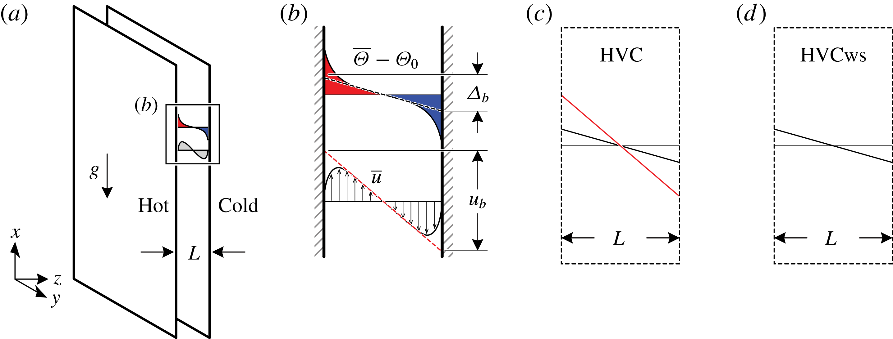
(a) Set-up of VC. (b) Illustration of the mean temperature profile (top) and mean streamwise velocity profile (bottom). Both mean profiles are statistically antisymmetric about the channel centreline. (c) Set-up of HVC with a mean temperature and velocity gradient. (d) Set-up of HVCws with only a mean temperature gradient. The black slopes in (c) and (d) represent the temperature gradient
 $\unicode[STIX]{x1D6E5}_{b}/L$
, whereas the red slope in (c) represents the uniform mean shear
 $u_{b}/L$
. Note that in (a), periodicity is applied in
 $x$
- and
 $y$
-directions only, whereas in (c) and (d), periodicity is applied in all three directions, illustrated by the dashed boundaries.
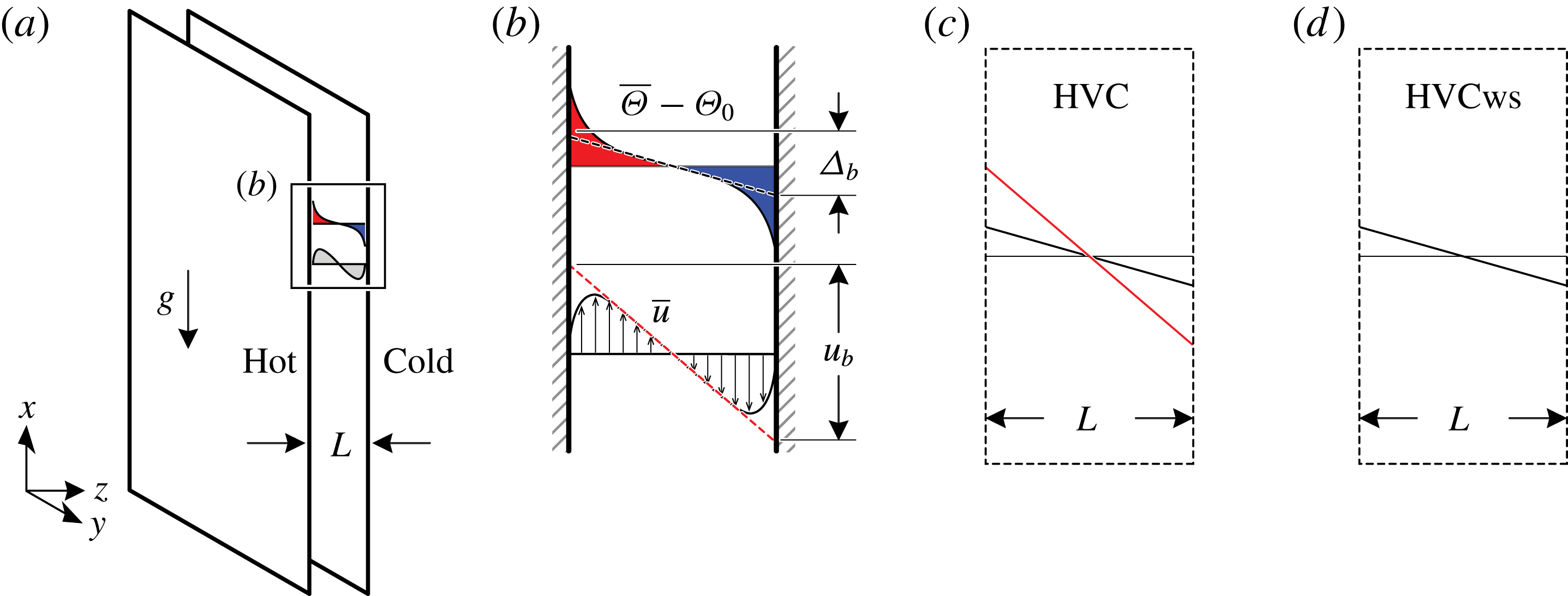
In the present study, we investigate the scaling relations of VC in a triply periodic domain (figure 2
c,d) using an approach that is similar to previous studies of bulk scaling for RBC (e.g. Lohse & Toschi Reference Lohse and Toschi2003; Calzavarini et al.
Reference Calzavarini, Lohse, Toschi and Tripiccione2005). The numerical set-up of this homogeneous flow is described in § 4. Our objective is to determine whether the asymptotic ultimate
 $1/2$
-power-law scaling can similarly be found in an idealised set-up of VC which is free of influences from the boundary layers. To achieve this, we adopted two approaches: (i) homogeneous VC with a constant mean temperature and velocity gradient in the horizontal direction, which we denote as HVC (figure 2
c), and (ii) homogeneous VC with only a constant horizontal mean temperature gradient and no velocity gradient (or shear), which we denote as HVCws (figure 2
d). Although the flow in (i) closely resembles the characteristics of the bulk flow in VC, we emphasise that the homogeneous and wall-bounded set-ups are different because for the homogeneous case, the energy transport to the walls is absent. In addition, the flow in (ii) without shear is evidently fictitious since a velocity gradient is present in the bulk of VC. In other words, both homogeneous cases (i) and (ii) are simplifications of VC, simplifications that are amenable to the
 $1/2$
-power-law scaling arguments as has been shown previously for homogeneous RBC (e.g. Lohse & Toschi Reference Lohse and Toschi2003).
The paper is structured as follows: we begin by describing the respective dynamical equations for HVC and HVCws in § 2, which are numerically solved. Using scaling arguments, we relate both HVC and HVCws with the asymptotic ultimate
 $1/2$
-power-law scaling in § 3. In § 4, we outline the numerical set-ups and direct numerical simulation (DNS) datasets, the latter being used to test the assumptions employed in our scaling arguments. Then, to assist comparisons with VC, we compare the dynamical length scales of HVC and HVCws with VC in § 5. In § 6, we compute the scaling of turbulent quantities of the homogeneous set-ups and show that
 $\mathit{Nu}$
and
 $\mathit{Re}$
appear to follow the
 $1/2$
-power-law scaling, just as in homogeneous RBC and consistent with the theoretical predictions by Kraichnan (Reference Kraichnan1962), the GL-theory and the scaling arguments in § 3. Inspired by the scaling of the turbulent quantities, we apply the insight gained to VC and find that the scaling of the turbulent bulk quantities in VC also exhibit the
 $1/2$
-power-law scaling. Finally, in § 7, we compare the stability of the solutions for HVCws and homogeneous RBC, the latter of which is known to exhibit unstable, so-called ‘elevator modes’ at low Rayleigh numbers. Such modes are associated with exponentially growing values of
 $\mathit{Nu}$
followed by sudden breakdowns (Calzavarini et al.
Reference Calzavarini, Lohse, Toschi and Tripiccione2005, Reference Calzavarini, Doering, Gibbon, Lohse, Tanabe and Toschi2006a
) and have been reported in similar studies, such as in laterally confined and axially homogeneous RBC (Schmidt et al.
Reference Schmidt, Calzavarini, Lohse, Toschi and Verzicco2012). In § 8, when we compared the stability analyses to data from our DNS of HVCws, we find that the unsteady solutions are also present in HVCws at low
 $\mathit{Ra}$
, but nonetheless both
 $\mathit{Nu}$
and
 $\mathit{Re}$
appear to follow the
 $1/2$
-power-law scaling.
2 Dynamical equations
We begin with the general form of the governing equations for VC, where we invoke the Boussinesq approximation so that the density fluctuations are considered small relative to the mean. The governing continuity, momentum and energy equations for the velocity field
 $u_{i}(x_{i},t)$
and the temperature field
 $\unicode[STIX]{x1D6E9}(x_{i},t)$
are respectively given by,
 $$\begin{eqnarray}\displaystyle {\displaystyle \frac{\unicode[STIX]{x2202}u_{j}}{\unicode[STIX]{x2202}x_{j}}} & = & \displaystyle 0,\end{eqnarray}$$
 $$\begin{eqnarray}\displaystyle {\displaystyle \frac{\unicode[STIX]{x2202}u_{i}}{\unicode[STIX]{x2202}t}}+{\displaystyle \frac{\unicode[STIX]{x2202}u_{j}u_{i}}{\unicode[STIX]{x2202}x_{j}}} & = & \displaystyle -{\displaystyle \frac{1}{\unicode[STIX]{x1D70C}_{0}}}{\displaystyle \frac{\unicode[STIX]{x2202}p}{\unicode[STIX]{x2202}x_{i}}}+\unicode[STIX]{x1D708}{\displaystyle \frac{\unicode[STIX]{x2202}^{2}u_{i}}{\unicode[STIX]{x2202}x_{j}^{2}}}+g\unicode[STIX]{x1D6FD}(\unicode[STIX]{x1D6E9}-\unicode[STIX]{x1D6E9}_{0})\unicode[STIX]{x1D6FF}_{i1},\end{eqnarray}$$
 $$\begin{eqnarray}\displaystyle {\displaystyle \frac{\unicode[STIX]{x2202}\unicode[STIX]{x1D6E9}}{\unicode[STIX]{x2202}t}}+{\displaystyle \frac{\unicode[STIX]{x2202}u_{i}\unicode[STIX]{x1D6E9}}{\unicode[STIX]{x2202}x_{i}}} & = & \displaystyle \unicode[STIX]{x1D705}{\displaystyle \frac{\unicode[STIX]{x2202}^{2}\unicode[STIX]{x1D6E9}}{\unicode[STIX]{x2202}x_{i}^{2}}}.\end{eqnarray}$$
The coordinate system
 $x$
,
 $y$
and
 $z$
(or
 $x_{1}$
,
 $x_{2}$
and
 $x_{3}$
) refers to the vertical streamwise direction that is opposite to gravity, spanwise and wall-normal directions, respectively. The pressure field is denoted by
 $p(x_{i},t)$
. For VC (see figure 2
a), we define
 $\unicode[STIX]{x1D6E9}_{0}=(T_{h}+T_{c})/2$
as the reference temperature,
 $\unicode[STIX]{x1D6E5}\equiv T_{h}-T_{c}$
the temperature difference between the two walls, which are separated by a distance
 $L$
, and
 $g$
as the gravitational acceleration. For the fluid, we specify
 $\unicode[STIX]{x1D6FD}$
as the coefficient of thermal expansion,
 $\unicode[STIX]{x1D708}$
as the kinematic viscosity and
 $\unicode[STIX]{x1D705}$
as the thermal diffusivity, all assumed to be independent of temperature. The Rayleigh and Prandtl numbers are then respectively defined as
 $$\begin{eqnarray}\displaystyle \mathit{Ra}\equiv g\unicode[STIX]{x1D6FD}\unicode[STIX]{x0394}L^{3}/(\unicode[STIX]{x1D708}\unicode[STIX]{x1D705}),\quad \mathit{Pr}\equiv \unicode[STIX]{x1D708}/\unicode[STIX]{x1D705}, & & \displaystyle\end{eqnarray}$$
and the Nusselt and Reynolds numbers are respectively defined as
 $$\begin{eqnarray}\displaystyle \mathit{Nu}\equiv JL/(\unicode[STIX]{x0394}\unicode[STIX]{x1D705}),\quad \mathit{Re}\equiv UL/\unicode[STIX]{x1D708}, & & \displaystyle\end{eqnarray}$$
where
 $J\equiv -\unicode[STIX]{x1D705}(\text{d}\overline{\unicode[STIX]{x1D6E9}}/\text{d}z)+\overline{w^{\prime }\unicode[STIX]{x1D6E9}^{\prime }}$
the horizontal heat flux and
 $U$
is a characteristic velocity scale. Equations (2.1a–c
) have been numerically solved in Ng et al. (Reference Ng, Ooi, Lohse and Chung2015) for no-slip and impermeable boundary conditions for the velocity field at the walls (in the plane
 $z=0$
and
 $z=L$
) and periodic boundary conditions in the
 $x$
- and
 $y$
-directions. The resulting mean streamwise velocity component (
 $\overline{u}=u-u^{\prime }$
) and mean temperature (
 $\overline{\unicode[STIX]{x1D6E9}}=\unicode[STIX]{x1D6E9}-\unicode[STIX]{x1D6E9}^{\prime }$
) are statistically antisymmetric about the channel centreline, as illustrated in figure 2(b). Here, we denote time- and
 $xy$
-plane-averaged quantities with an overbar, and the corresponding fluctuating part with a prime. In the channel centre of VC, both
 $\text{d}\overline{u}/\text{d}z$
and
 $\text{d}\overline{\unicode[STIX]{x1D6E9}}/\text{d}z$
are finite and possesses the same sign. Note that in VC,
 $\overline{u}$
is a persistent non-zero-mean quantity, which is different to RBC: for a sufficiently long time average, it can be shown that the wall-parallel-averaged velocity components in RBC are statistically zero (e.g. van Reeuwijk, Jonker & Hanjalić Reference van Reeuwijk, Jonker and Hanjalić2008).
For the present study, we are interested in two numerical set-ups that are different from VC. The new set-ups are defined such that they allow us to directly test the
 $1/2$
-power scaling relations described in (1.1). From this line of reasoning, the associated governing equations of the new set-ups should be expected to obey the scaling arguments of Kraichnan (Reference Kraichnan1962) and Grossmann & Lohse (Reference Grossmann and Lohse2000), and in the spirit of deriving (1.1). In short, the key idea here is to design numerical set-ups that only solve the fluctuating components of VC, which conveniently emulates the turbulent bulk-dominated conditions expected in the asymptotic ultimate regime of thermal convection at very high
 $\mathit{Ra}$
(Grossmann & Lohse Reference Grossmann and Lohse2000). To this end, we describe two set-ups for VC, i.e. HVC and HVCws, which are inspired by the so-called homogeneous configurations for RBC of Lohse & Toschi (Reference Lohse and Toschi2003) and Calzavarini et al. (Reference Calzavarini, Lohse, Toschi and Tripiccione2005, Reference Calzavarini, Doering, Gibbon, Lohse, Tanabe and Toschi2006a
). Different to homogeneous RBC, the HVC and HVCws set-ups described in the following sections are subjected to a mean horizontal temperature (or buoyancy) gradient, which is orthogonal to gravity.
2.1 Homogeneous vertical natural convection with shear (HVC)
For HVC, we assume that the flow is decomposed into constant mean gradients and fluctuations. These assumptions are notionally similar to the flow conditions in the channel centre of VC, as illustrated in figure 2(b,c). To describe the numerical approach, we also make use of the equation of state for gases,
 $\unicode[STIX]{x1D6FD}(\unicode[STIX]{x1D6E9}-\unicode[STIX]{x1D6E9}_{0})\approx -(1/\unicode[STIX]{x1D70C}_{0})(\unicode[STIX]{x1D70C}-\unicode[STIX]{x1D70C}_{0})$
and introduce
 $b$
the buoyancy variable. Therefore, following Chung & Matheou (Reference Chung and Matheou2012), we write
 $$\begin{eqnarray}\displaystyle -(g/\unicode[STIX]{x1D70C}_{0})(\unicode[STIX]{x1D70C}-\unicode[STIX]{x1D70C}_{0}) & = & \displaystyle N^{2}x_{3}+b^{\prime },\end{eqnarray}$$
 $$\begin{eqnarray}\displaystyle u_{i} & = & \displaystyle S\unicode[STIX]{x1D6FF}_{i1}x_{3}+u_{i}^{\prime },\end{eqnarray}$$
 $$\begin{eqnarray}\displaystyle p+\unicode[STIX]{x1D70C}_{0}gx_{1} & = & \displaystyle p^{\prime },\end{eqnarray}$$
 $N^{2}\equiv \text{d}\overline{b}/\text{d}z=g\unicode[STIX]{x1D6FD}\,\text{d}\overline{\unicode[STIX]{x1D6E9}}/\text{d}z$
is the constant mean buoyancy gradient,
 $S\equiv \text{d}\overline{u}/\text{d}z$
the (temporally) uniform mean shear and
 $u_{i}^{\prime }$
,
 $b^{\prime }$
and
 $p^{\prime }$
are the fluctuations of velocity, buoyancy and pressure, respectively. Substituting (2.4) into (2.1a
), we obtain
 $$\begin{eqnarray}\displaystyle {\displaystyle \frac{\unicode[STIX]{x2202}u_{j}^{\prime }}{\unicode[STIX]{x2202}x_{j}}} & = & \displaystyle 0,\end{eqnarray}$$
 $$\begin{eqnarray}\displaystyle {\displaystyle \frac{\unicode[STIX]{x2202}b^{\prime }}{\unicode[STIX]{x2202}t}}+N^{2}u_{3}^{\prime }+{\displaystyle \frac{\unicode[STIX]{x2202}u_{j}^{\prime }b^{\prime }}{\unicode[STIX]{x2202}x_{j}}}+S\unicode[STIX]{x1D6FF}_{j1}x_{3}{\displaystyle \frac{\unicode[STIX]{x2202}b^{\prime }}{\unicode[STIX]{x2202}x_{j}}} & = & \displaystyle \unicode[STIX]{x1D705}{\displaystyle \frac{\unicode[STIX]{x2202}^{2}b^{\prime }}{\unicode[STIX]{x2202}x_{j}^{2}}}\end{eqnarray}$$
 $$\begin{eqnarray}\displaystyle {\displaystyle \frac{\unicode[STIX]{x2202}u_{i}^{\prime }}{\unicode[STIX]{x2202}t}}+S\unicode[STIX]{x1D6FF}_{i1}u_{3}^{\prime }+{\displaystyle \frac{\unicode[STIX]{x2202}u_{j}^{\prime }u_{i}^{\prime }}{\unicode[STIX]{x2202}x_{j}}}+S\unicode[STIX]{x1D6FF}_{j1}x_{3}{\displaystyle \frac{\unicode[STIX]{x2202}u_{i}^{\prime }}{\unicode[STIX]{x2202}x_{j}}} & = & \displaystyle -{\displaystyle \frac{1}{\unicode[STIX]{x1D70C}_{0}}}{\displaystyle \frac{\unicode[STIX]{x2202}p^{\prime }}{\unicode[STIX]{x2202}x_{i}}}+\unicode[STIX]{x1D708}{\displaystyle \frac{\unicode[STIX]{x2202}^{2}u_{i}^{\prime }}{\unicode[STIX]{x2202}x_{j}^{2}}}+(N^{2}x_{3}+b^{\prime })\unicode[STIX]{x1D6FF}_{i1}.\end{eqnarray}$$
 $\unicode[STIX]{x1D709}_{i}(x_{i},t)=x_{i}-St\unicode[STIX]{x1D6FF}_{i1}x_{3}$
is introduced to transform the dependent variables
 $\{b^{\prime },u_{i}^{\prime },p^{\prime }\}(x_{i},t)=\{\widetilde{b},\widetilde{u}_{i},\widetilde{p}\}(\unicode[STIX]{x1D709}_{i}(x_{i},t),t)$
to convert (2.5) to
 $$\begin{eqnarray}\displaystyle {\displaystyle \frac{\unicode[STIX]{x2202}\widetilde{u}_{j}}{\unicode[STIX]{x2202}\widetilde{\unicode[STIX]{x1D709}}_{j}}} & = & \displaystyle 0,\end{eqnarray}$$
 $$\begin{eqnarray}\displaystyle {\displaystyle \frac{\unicode[STIX]{x2202}\widetilde{b}}{\unicode[STIX]{x2202}t}}+N^{2}\widetilde{u}_{3}+{\displaystyle \frac{\unicode[STIX]{x2202}\widetilde{u}_{j}\widetilde{b}}{\unicode[STIX]{x2202}\widetilde{\unicode[STIX]{x1D709}}_{j}}} & = & \displaystyle \unicode[STIX]{x1D705}{\displaystyle \frac{\unicode[STIX]{x2202}^{2}\widetilde{b}}{\unicode[STIX]{x2202}\widetilde{\unicode[STIX]{x1D709}}_{j}^{2}}},\end{eqnarray}$$
 $$\begin{eqnarray}\displaystyle {\displaystyle \frac{\unicode[STIX]{x2202}\widetilde{u}_{i}}{\unicode[STIX]{x2202}t}}+S\unicode[STIX]{x1D6FF}_{i1}\widetilde{u}_{3}+{\displaystyle \frac{\unicode[STIX]{x2202}\widetilde{u}_{j}\widetilde{u}_{i}}{\unicode[STIX]{x2202}\widetilde{\unicode[STIX]{x1D709}}_{j}}} & = & \displaystyle -{\displaystyle \frac{1}{\unicode[STIX]{x1D70C}_{0}}}{\displaystyle \frac{\unicode[STIX]{x2202}\widetilde{p}}{\unicode[STIX]{x2202}\widetilde{\unicode[STIX]{x1D709}}_{i}}}+\unicode[STIX]{x1D708}{\displaystyle \frac{\unicode[STIX]{x2202}^{2}\widetilde{u}_{i}}{\unicode[STIX]{x2202}\widetilde{\unicode[STIX]{x1D709}}_{j}^{2}}}+(N^{2}\unicode[STIX]{x1D709}_{3}+\widetilde{b})\unicode[STIX]{x1D6FF}_{i1},\end{eqnarray}$$
 $\unicode[STIX]{x2202}/\unicode[STIX]{x2202}\widetilde{\unicode[STIX]{x1D709}}_{i}\equiv \unicode[STIX]{x2202}/\unicode[STIX]{x2202}\unicode[STIX]{x1D709}_{i}-St\unicode[STIX]{x1D6FF}_{i3}\unicode[STIX]{x2202}/\unicode[STIX]{x2202}\unicode[STIX]{x1D709}_{1}$
.
The transformation from (2.5) to (2.6) allows us to numerically solve (2.6) in a triply periodic domain provided
 $N^{2}\unicode[STIX]{x1D709}_{3}$
the non-periodic term on the right-hand side of (2.6c
), which acts on the streamwise momentum, can be neglected. This is satisfied if
 $|N^{2}\unicode[STIX]{x1D709}_{3}|\ll |\widetilde{b}|$
. Estimating
 $|\widetilde{b}|=O(b_{rms})$
, where
 $b_{rms}$
is the time- and volume-averaged root-mean-square (r.m.s.) of
 $b$
, the inequality then holds true for scales in the
 $z$
-direction that are smaller than
 $b_{rms}/N^{2}(=\unicode[STIX]{x1D6E9}_{rms}(\text{d}\overline{\unicode[STIX]{x1D6E9}}/\text{d}z)^{-1})$
. There is no straightforward method to determine beforehand if
 $b_{rms}/N^{2}$
is larger or smaller than
 $L_{z}$
without performing the homogeneous simulations. As a start, we omit the non-periodic term from our DNS, noting that this is a necessary numerical approximation. On the other hand, if
 $b_{rms}/N^{2}<L_{z}$
, the solutions based on the DNS without the non-periodic term are still meaningful, provided we focus only on the dynamics of the scales that are
 ${\lesssim}b_{rms}/N^{2}$
. Indeed, we will show in § 6.1 that
 $b_{rms}/N^{2}<L_{z}$
for the homogeneous cases, which we then further enforce in our calculations of the Nusselt and Reynolds number in § 6.2, where we apply a spectral filter to the Nusselt and Reynolds number using a cutoff length of the order of
 $b_{rms}/N^{2}$
, smaller than
 $L_{z}$
.
The solutions to (2.6) without the non-periodic term describe the evolution of the fluctuating quantities of VC under the influence of a prescribed mean buoyancy gradient and mean shear. We acknowledge that the aforementioned assumptions are merely simplifications since both the mean shear
 $S$
and the buoyancy gradient
 $N^{2}$
are in principle the responding parameters of the bulk flow of VC; the boundary layers that form at the walls determine
 $S$
and
 $N^{2}$
. Thus, an explicit relation between
 $S$
and
 $N^{2}$
is presently unknown, at least to our knowledge. Similarly, in the case of HVC, both
 $S$
and
 $N^{2}$
are not known a priori but must be prescribed. (This is detailed in § 4). We emphasise that the formulation for HVC above is not an attempt to simulate the bulk flow of VC – it is instead an idealised numerical model that is designed to test the
 $1/2$
-power-law scalings of (1.1).
2.2 Homogeneous vertical natural convection without shear (HVCws)
In addition to HVC, HVCws is an alternative numerical set-up that can test the
 $1/2$
-power-law scalings by assuming that the mean shear component
 $S$
in (2.4b
) is zero, i.e.
 $u_{i}=u_{i}^{\prime }$
. It follows that the homogeneous simulations without shear can be conducted in the same triply periodic domain as HVC, but with the second term on the left-hand side of (2.6c
), which is
 $S\unicode[STIX]{x1D6FF}_{i1}\widetilde{u}_{3}$
, set to zero.
This assumption of the zero-mean shear is inspired by similar homogeneous studies for RBC (e.g. Lohse & Toschi Reference Lohse and Toschi2003; Calzavarini et al.
Reference Calzavarini, Lohse, Toschi and Tripiccione2005). For VC, the zero-mean-shear assumption is evidently fictitious since in reality, a mean flow is present. However, we make this assumption for the sake of convenience since we will show later in § 3.3 that, with
 $S=0$
, the
 $1/2$
-power-law scaling arguments appear to hold more naturally. Note that for past studies on homogeneous RBC (e.g. Lohse & Toschi Reference Lohse and Toschi2003; Calzavarini et al.
Reference Calzavarini, Lohse, Toschi and Tripiccione2005), the zero-mean-shear assumption inherently holds because the mean velocity components for RBC are zero. The zero-mean-shear assumption in RBC also implies that, in principle, the homogeneous RBC set-up would be directly comparable to the HVCws set-up, in contrast to the more phenomenologically accurate HVC set-up.
3 The relationship between the homogeneous set-ups and the 1/2-power-law asymptotic ultimate scaling
3.1 Definitions of the dimensionless numbers for the bulk
Based on the set-up for HVC and HVCws, we will now attempt to establish a priori the expected power-law scaling for
 $\mathit{Nu}$
and
 $\mathit{Re}$
in terms of
 $\mathit{Ra}$
and
 $\mathit{Pr}$
. Specifically, we are interested to determine whether the
 $1/2$
-power-law scalings described in (1.1) could also be expected for the homogeneous cases. Our approach follows the same scaling arguments as described in Grossmann & Lohse (Reference Grossmann and Lohse2000) for the asymptotic ultimate regime, which is referred in their work as the bulk-dominated regime for low-
 $\mathit{Pr}$
thermal convection (regime
 $IV_{l}$
), i.e. when
 $\mathit{Pr}\leqslant 1$
.
Before proceeding further, we first need to redefine the Rayleigh, Nusselt and Reynolds numbers for the homogeneous set-ups, i.e. (2.2a
) and (2.3), since the temperature scale
 $\unicode[STIX]{x1D6E5}$
and the characteristic velocity scale
 $U$
are undefined for HVC and HVCws. The temperature scale
 $\unicode[STIX]{x1D6E5}$
in the Nusselt and Rayleigh numbers refers to the imposed temperature difference, and so we adopt
 $\unicode[STIX]{x1D6E5}\equiv \unicode[STIX]{x1D6E5}_{b}\equiv -(\text{d}\overline{\unicode[STIX]{x1D6E9}}/\text{d}z)L$
. The velocity scale
 $U$
in the Reynolds number measures the system response, which are the velocity fluctuations and so we can define
 $U\equiv u_{rms}$
, where
 $u_{rms}$
is the time- and volume-averaged root-mean-square of the streamwise velocity fluctuations. Therefore, we recast
 $\mathit{Ra}$
,
 $\mathit{Nu}$
and
 $\mathit{Re}$
for the homogeneous set-ups as
 $$\begin{eqnarray}\displaystyle \mathit{Ra}_{b}\equiv g\unicode[STIX]{x1D6FD}\unicode[STIX]{x1D6E5}_{b}L^{3}/(\unicode[STIX]{x1D708}\unicode[STIX]{x1D705}),\quad \mathit{Nu}_{b}\equiv JL/(\unicode[STIX]{x1D6E5}_{b}\unicode[STIX]{x1D705}),\quad \mathit{Re}_{b}\equiv u_{rms}L/\unicode[STIX]{x1D708}. & & \displaystyle\end{eqnarray}$$
To distinguish (3.1) from the definitions for VC, we adopt the subscript
 $b$
to refer to the bulk-related quantities in the homogeneous flow. The length scale parameter
 $L$
is presently undefined, but for similar homogeneous studies of shear turbulence, Sekimoto, Dong & Jiménez (Reference Sekimoto, Dong and Jiménez2016) have shown that homogeneous flows are always ‘minimal’ and constrained by the shortest domain length. As such, we will later employ this definition for
 $L$
in § 4 for computing (3.1), but in the scaling arguments to follow, a different choice of
 $L$
simply affects the prefactors of the scaling arguments and not the exponent of the power law. Therefore, for the purposes of this section, the choice of
 $L$
is immaterial.
3.2
 $\mathit{Ra}$
-scaling in HVC

Starting with HVC, we consider the time- and volume-averaged kinetic and thermal dissipation rates which are obtained by manipulating (2.5) without the non-periodic term on the right-hand side of (2.5c ),
 $$\begin{eqnarray}\displaystyle \langle \unicode[STIX]{x1D700}_{u^{\prime }}\rangle =\unicode[STIX]{x1D6FD}g\langle u^{\prime }\unicode[STIX]{x1D6E9}^{\prime }\rangle -S\langle u^{\prime }w^{\prime }\rangle ,\quad \langle \unicode[STIX]{x1D700}_{\unicode[STIX]{x1D6E9}^{\prime }}\rangle =(\unicode[STIX]{x1D6E5}_{b}/L)\langle w^{\prime }\unicode[STIX]{x1D6E9}^{\prime }\rangle . & & \displaystyle\end{eqnarray}$$
The notation
 $\langle (\cdot )\rangle$
denotes time and volume averaging. Next, we write (3.2) explicitly in terms of (3.1). However, before doing so, we recognise that the two terms on the right-hand side of (3.2a
) are not known explicitly in terms of (3.1). Thus, we make two necessary assumptions which we verify later in § 6.1: the first assumption is that
 $\langle u^{\prime }\unicode[STIX]{x1D6E9}^{\prime }\rangle \sim \langle w^{\prime }\unicode[STIX]{x1D6E9}^{\prime }\rangle$
and the second assumption is that
 $\langle u^{\prime }w^{\prime }\rangle \sim u_{c}^{2}\equiv \langle \unicode[STIX]{x1D700}_{u^{\prime }}\rangle /|S|$
, where
 $u_{c}$
is the Corrsin velocity scale.
A physical interpretation of the first assumption is warranted at this point: because the driving heat flux is perpendicular to the gravity vector in our set-up, we assume that a relatively greater and uniform mixing is present in HVC compared to homogeneous RBC. Thus, the HVC flow presumably generates vertical and horizontal small scales (in the direction of the driving heat flux) that are magnitude-wise comparable. A careful comparison between HVC and homogeneous RBC datasets at matched
 $\mathit{Ra}_{b}$
is warranted to verify this relation. The first assumption is also felicitous and essential since the relation between the turbulent horizontal heat flux and the turbulent vertical heat flux is inherently unknown for VC, which is in contrast to RBC where both the turbulent driving and responding heat fluxes are parallel to gravity.
With the two assumptions, equation (3.2a
) can be written as
 $\langle \unicode[STIX]{x1D700}_{u^{\prime }}\rangle \sim \unicode[STIX]{x1D6FD}g\langle w^{\prime }\unicode[STIX]{x1D6E9}^{\prime }\rangle -S(\langle \unicode[STIX]{x1D700}_{u^{\prime }}\rangle /|S|)$
and so we can explicitly write (3.2) as
 $$\begin{eqnarray}\displaystyle \langle \unicode[STIX]{x1D700}_{u^{\prime }}\rangle \sim {\displaystyle \frac{\unicode[STIX]{x1D708}^{3}}{L^{4}}}\mathit{Ra}_{b}\mathit{Pr}^{-2}(\mathit{Nu}_{b}-1),\quad \langle \unicode[STIX]{x1D700}_{\unicode[STIX]{x1D6E9}^{\prime }}\rangle =\unicode[STIX]{x1D705}{\displaystyle \frac{\unicode[STIX]{x1D6E5}_{b}^{2}}{L^{2}}}(\mathit{Nu}_{b}-1). & & \displaystyle\end{eqnarray}$$
Next, we model the global-averaged dissipation rates on the left-hand side of (3.2) following the dimensional arguments for the turbulence cascade in fully developed turbulence, where the dissipation rate of turbulent fluctuations scale with the energy of the largest eddies of the order of
 $u_{rms}^{2}$
over a time scale
 $L/u_{rms}$
(Pope Reference Pope2000, ch. 6). By analogy, the dissipation rate of thermal variance scales with the largest eddies with variance
 $\unicode[STIX]{x1D6E9}_{rms}^{2}$
over a time scale
 $L/u_{rms}$
. Thus,
 $$\begin{eqnarray}\displaystyle \langle \unicode[STIX]{x1D700}_{u^{\prime }}\rangle \sim {\displaystyle \frac{u_{rms}^{3}}{L}}={\displaystyle \frac{\unicode[STIX]{x1D708}^{3}}{L^{4}}}\mathit{Re}_{b}^{3},\quad \langle \unicode[STIX]{x1D700}_{\unicode[STIX]{x1D6E9}^{\prime }}\rangle \sim {\displaystyle \frac{u_{rms}\unicode[STIX]{x1D6E9}_{rms}^{2}}{L}}=\unicode[STIX]{x1D705}{\displaystyle \frac{\unicode[STIX]{x1D6E9}_{rms}^{2}}{L^{2}}}\mathit{Pr}\mathit{Re}_{b}. & & \displaystyle\end{eqnarray}$$
(cf. Grossmann & Lohse Reference Grossmann and Lohse2000). We can now match (3.3a ) with (3.4a ) and (3.3b ) with (3.4b ) and eliminate common terms to obtain,
 $$\begin{eqnarray}\displaystyle \mathit{Ra}_{b}\mathit{Pr}^{-2}(\mathit{Nu}_{b}-1)\sim \mathit{Re}_{b}^{3},\quad \unicode[STIX]{x1D6E5}_{b}^{2}(\mathit{Nu}_{b}-1)\sim \unicode[STIX]{x1D6E9}_{rms}^{2}\mathit{Pr}\mathit{Re}_{b}. & & \displaystyle\end{eqnarray}$$
Equation (3.5b
) can be simplified if we assume that
 $\unicode[STIX]{x1D6E5}_{b}\sim \unicode[STIX]{x1D6E9}_{rms}$
and thus, we can manipulate (3.5) to obtain
 $$\begin{eqnarray}\displaystyle \mathit{Nu}_{b}\sim \mathit{Ra}_{b}^{1/2}\mathit{Pr}^{1/2},\quad \mathit{Re}_{b}\sim \mathit{Ra}_{b}^{1/2}\mathit{Pr}^{-1/2}, & & \displaystyle\end{eqnarray}$$
which is the same as the
 $1/2$
-power-law expressions derived in (2.19) and (2.20) of Grossmann & Lohse (Reference Grossmann and Lohse2000), similar to the asymptotic Kraichnan regime (Kraichnan Reference Kraichnan1962).
Alternatively, we can emphasise the role of the mean components on the turbulent dissipation rates (as shown in Ng et al.
Reference Ng, Ooi, Lohse and Chung2015) by defining the energy of the kinetic and thermal eddies based on
 $u_{b}$
and
 $\unicode[STIX]{x1D6E5}_{b}$
, where
 $u_{b}\equiv -SL_{z}$
. Therefore, instead of (3.4), the global-averaged dissipation rates on the left-hand side of (3.2) may be modelled as
 $$\begin{eqnarray}\displaystyle \langle \unicode[STIX]{x1D700}_{u^{\prime }}\rangle \sim {\displaystyle \frac{u_{b}^{3}}{L}}={\displaystyle \frac{\unicode[STIX]{x1D708}^{3}}{L^{4}}}\mathit{Re}_{b}^{3}\left({\displaystyle \frac{u_{b}^{3}}{u_{rms}^{3}}}\right),\quad \langle \unicode[STIX]{x1D700}_{\unicode[STIX]{x1D6E9}^{\prime }}\rangle \sim {\displaystyle \frac{u_{b}\unicode[STIX]{x1D6E5}_{b}^{2}}{L}}=\unicode[STIX]{x1D705}{\displaystyle \frac{\unicode[STIX]{x1D6E5}_{b}^{2}}{L^{2}}}\mathit{Pr}\mathit{Re}_{b}\left({\displaystyle \frac{u_{b}}{u_{rms}}}\right). & & \displaystyle\end{eqnarray}$$
Equation (3.7) can be simplified if we assume
 $u_{b}\sim u_{rms}$
. Thus, we can match (3.3a
) with (3.7a
) and (3.3b
) with (3.7b
), as before, and recover the same
 $1/2$
-power-law scaling of (3.6). Both assumptions
 $\unicode[STIX]{x1D6E5}_{b}\sim \unicode[STIX]{x1D6E9}_{rms}$
and
 $u_{b}\sim u_{rms}$
are reasonable in the absence of walls, since the fluctuating quantities respond directly to the input quantities
 $\unicode[STIX]{x1D6E5}_{b}$
and
 $u_{b}$
, which are constant (Calzavarini et al.
Reference Calzavarini, Lohse, Toschi and Tripiccione2005). When walls are present, a different treatment is necessary and would depend on the distance from the wall, see for example the mixing length model proposed in Shishkina et al. (Reference Shishkina, Horn, Emran and Ching2017).
In summary, the governing equations for HVC appear to provide a natural
 $1/2$
-power-law scaling in the spirit of the GL-theory formulation. However, we reiterate that the homogeneous set-up is merely an idealisation which enables us to test the
 $1/2$
-power-law scaling and does not explicitly model the flow at the channel centre of VC. The scaling arguments above are consistent with the approach previously discussed by Lohse & Toschi (Reference Lohse and Toschi2003) for homogeneous RBC.
3.3
$\mathit{Ra}$
-scaling in HVCws

When the shear is absent in the homogeneous set-up, the scaling arguments are relatively more straightforward because
 $S=0$
. That is, by manipulating (2.5) without the terms containing
 $S$
and the non-periodic term, we obtain the global-averaged kinetic and thermal dissipation rates
 $$\begin{eqnarray}\displaystyle \langle \unicode[STIX]{x1D700}_{u^{\prime }}\rangle =\unicode[STIX]{x1D6FD}g\langle u^{\prime }\unicode[STIX]{x1D6E9}^{\prime }\rangle ,\quad \langle \unicode[STIX]{x1D700}_{\unicode[STIX]{x1D6E9}^{\prime }}\rangle =(\unicode[STIX]{x1D6E5}_{b}/L)\langle w^{\prime }\unicode[STIX]{x1D6E9}^{\prime }\rangle . & & \displaystyle\end{eqnarray}$$
We can now repeat the only assumption that
 $\langle u^{\prime }\unicode[STIX]{x1D6E9}^{\prime }\rangle \sim \langle w^{\prime }\unicode[STIX]{x1D6E9}^{\prime }\rangle$
to rewrite (3.8) explicitly as
 $$\begin{eqnarray}\displaystyle \langle \unicode[STIX]{x1D700}_{u^{\prime }}\rangle \sim {\displaystyle \frac{\unicode[STIX]{x1D708}^{3}}{L^{4}}}\mathit{Ra}_{b}\mathit{Pr}^{-2}(\mathit{Nu}_{b}-1),\quad \langle \unicode[STIX]{x1D700}_{\unicode[STIX]{x1D6E9}^{\prime }}\rangle =\unicode[STIX]{x1D705}{\displaystyle \frac{\unicode[STIX]{x1D6E5}_{b}^{2}}{L^{2}}}(\mathit{Nu}_{b}-1), & & \displaystyle\end{eqnarray}$$
which is the same as (3.3) for HVC.
Next, since only the fluctuations are relevant for HVCws, the global-averaged dissipation rates on the left-hand side of (3.8) scale according to (3.4). Lastly, by matching (3.9) and (3.4), and manipulating the dimensionless terms, we again obtain
 $$\begin{eqnarray}\displaystyle \mathit{Nu}_{b}\sim \mathit{Ra}_{b}^{1/2}\mathit{Pr}^{1/2},\quad \mathit{Re}_{b}\sim \mathit{Ra}_{b}^{1/2}\mathit{Pr}^{-1/2}, & & \displaystyle\end{eqnarray}$$
which is the same as (3.6).
From the scaling arguments above, we conclude that both HVC and HVCws are expected to exhibit
 $1/2$
-power-law scaling exponents, provided the assumptions that
 $\langle u^{\prime }\unicode[STIX]{x1D6E9}^{\prime }\rangle \sim \langle w^{\prime }\unicode[STIX]{x1D6E9}^{\prime }\rangle$
,
 $\unicode[STIX]{x1D6E5}_{b}\sim \unicode[STIX]{x1D6E9}_{rms}$
and
 $u_{b}\sim u_{rms}$
hold.
4 Computational parameters
We now proceed to describe the numerical simulations of the homogeneous set-ups. The simulations are performed in a triply periodic box with a height that is twice its horizontal width, but with its depth that is half of its horizontal width:
 $L_{x}=4L_{y}=2L_{z}$
(see figure 2
c,d). The longer streamwise length is in anticipation of the streamwise-elongated structures in the presence of shear (Chung & Matheou Reference Chung and Matheou2012), i.e. for the case of HVC, whereas the shorter spanwise length used in our simulations fulfils the limits proposed for stationary shear flows (e.g. Sekimoto et al.
Reference Sekimoto, Dong and Jiménez2016). A qualitative assessment on the sensitivity of the domain sizes is provided in appendix A. Both the longer streamwise box height and shorter spanwise depth are necessary for the homogeneous set-up in the presence of shear, which makes our domain different to previous studies on homogeneous thermal convection, such as for homogeneous RBC which were conducted in a box with equal height, width and depth (e.g. Lohse & Toschi Reference Lohse and Toschi2003; Calzavarini et al.
Reference Calzavarini, Lohse, Toschi and Tripiccione2005, Reference Calzavarini, Doering, Gibbon, Lohse, Tanabe and Toschi2006a
). For consistency and to assist comparison, we employ the box dimensions for HVC to the cases of HVCws. Since
 $L_{y}$
is the shortest box dimension for our set-up, the largest structures of the flow are determined by this domain length (cf. appendix A) and so, we adopt
 $L\equiv L_{y}$
in our definition of
 $\mathit{Ra}_{b}$
in (2.2a
) and also for the simulation parameters described below. The spanwise-domain-based definition of
 $\mathit{Ra}_{b}$
for the homogeneous set-ups also allows for a meaningful comparison with the bulk of VC and the associated channel-width-based definition of the Rayleigh number, where the bulk flow is determined by the distant boundary layers. All of our simulations employ equal grid spacings in all three directions.
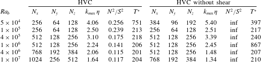
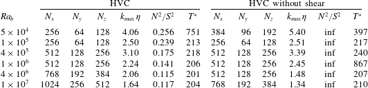
Simulation parameters of the present DNS cases for HVC and HVC without shear. For all cases,
 $L_{x}=4L_{y}=2L_{z}$
. Here,
 $k_{max}$
is the maximum dealiased wavenumber magnitude and
 $T^{\ast }\equiv T_{samp}U_{\unicode[STIX]{x1D6E5}}/L_{y}$
, where
 $T_{samp}$
is the sampling interval.
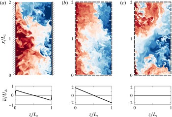
Streamwise-wall-normal visualisations of
 $\unicode[STIX]{x1D6E9}$
the instantaneous temperature field at matched Rayleigh number (
 $\mathit{Ra}_{b}\approx 10^{7}$
) for (a) VC, (b) HVC and (c) HVCws, highlighting the difference between homogeneous set-ups and VC. Temperature is decreasing from red to blue and the three plots share the same colour map. The tilted structures in (b) are reminiscent of the tilted structures in (a) at
 $z\approx 0.5L_{z}$
, but the structures in (c) bear little resemblance to the structures in (a) and (b). The respective mean velocity profiles are shown beneath the visualisations. As in figure 2, the hatched boundaries in (a) represent walls and the dashed boundaries in (b) and (c) represent periodic boundary conditions. Note that in the visualisation in (a) only a quarter section of VC is reproduced from the DNS of Ng et al. (Reference Ng, Ooi, Lohse and Chung2015).

Table 1 summarises the relevant simulation parameters used in this study. The simulation adopts a Fourier pseudospectral method (with the typical 2/3-rule for dealiasing in wavenumber space) that is stepped in time using the low-storage third-order Runge–Kutta scheme (cf. Chung & Matheou Reference Chung and Matheou2012) at the time stepping interval
 $\unicode[STIX]{x1D6E5}_{t}=\text{CFL}~\text{max}_{i}(\unicode[STIX]{x1D6E5}_{i}/u_{i}^{\prime })$
, where we have set
 $\text{CFL}=0.9$
and
 $\unicode[STIX]{x1D6E5}_{i}$
is the dealiased grid spacing in each direction. The data from the simulations are sampled for at least approximately 200 turnover times based on the free-fall period
 $t_{f}\equiv L_{y}/U_{\unicode[STIX]{x1D6E5}}$
, where
 $U_{\unicode[STIX]{x1D6E5}}\equiv \sqrt{g\unicode[STIX]{x1D6FD}\unicode[STIX]{x1D6E5}_{b}L_{y}}$
, after discarding at least 99 turnover times. When compared to the diffusive time scale
 $t_{\unicode[STIX]{x1D705}}\equiv L_{y}^{2}/\unicode[STIX]{x1D705}$
, it can be shown that
 $t_{\unicode[STIX]{x1D705}}=(\mathit{Ra}_{b}\mathit{Pr})^{1/2}t_{f}$
, reflecting that the free-fall time scale is much faster than the diffusive time scale by a factor of
 $(\mathit{Ra}_{b}\mathit{Pr})^{1/2}$
. In the present study, the simulations are resolved up to at least
 $k_{max}\unicode[STIX]{x1D702}\approx 1.34$
, where
 $k_{max}$
is the maximum dealiased wavenumber magnitude,
 $\unicode[STIX]{x1D702}\equiv (\unicode[STIX]{x1D708}^{3}/\langle \unicode[STIX]{x1D700}_{u^{\prime }}\rangle )^{1/4}$
is the Kolmogorov scale and
 $\langle \unicode[STIX]{x1D700}_{u^{\prime }}\rangle \equiv \unicode[STIX]{x1D708}\langle (\unicode[STIX]{x2202}u_{i}^{\prime }/\unicode[STIX]{x2202}x_{j})^{2}\rangle$
. The values of
 $\langle \unicode[STIX]{x1D700}_{u^{\prime }}\rangle$
used in table 1 and throughout this paper are calculated explicitly from the gradients of the velocity fluctuations in our DNS. For a comparison with the approximations for
 $\langle \unicode[STIX]{x1D700}_{u^{\prime }}\rangle$
, i.e. the right-hand side of (3.3a
) in the case of HVC and the right-hand side of (3.9a
) in the case of HVCws, we have included a discussion in appendix B. For HVCws, we selected a finer resolution for the lowest
 $\mathit{Ra}_{b}$
case (
 $=5\times 10^{4}$
), such that it is comparable to the resolution used in past numerical studies of low-
 $\mathit{Ra}_{b}$
for homogeneous RBC (e.g. Calzavarini et al.
Reference Calzavarini, Doering, Gibbon, Lohse, Tanabe and Toschi2006a
). We also note that for HVCws, different choices of resolution will affect the maximum value
 $\mathit{Nu}_{b}$
. The counter-intuitive matter of grid sensitivity has been previously highlighted, for example by Calzavarini et al. (Reference Calzavarini, Doering, Gibbon, Lohse, Tanabe and Toschi2006a
), and also found and explained by Schmidt et al. (Reference Schmidt, Calzavarini, Lohse, Toschi and Verzicco2012) for axially homogeneous RBC. Similar to Schmidt et al. (Reference Schmidt, Calzavarini, Lohse, Toschi and Verzicco2012), we find that the value of
 $\mathit{Nu}_{b}$
is lower when a coarser resolution is used. For consistency with previous studies, here we only report the results from higher-resolution simulations.
For the HVC cases, 2 additional parameters need to be determined, namely
 $N^{2}$
and
 $S$
. The selection of the values of
 $N^{2}$
and
 $S$
for the HVC cases are not intuitive since there are no boundary layers to set the values, thus, an explicit relation between
 $N^{2}$
and
 $S$
as a function of
 $\mathit{Ra}_{b}$
are unknown. For the lack of a better justification, we define
 $N^{2}$
and
 $S$
for HVC based on the channel-centre gradients for VC from the DNS dataset of Ng et al. (Reference Ng, Ooi, Lohse and Chung2015). That is, we define
 $N^{2}\equiv g\unicode[STIX]{x1D6FD}(\text{d}\overline{\unicode[STIX]{x1D6E9}}/\text{d}z)|_{c}$
and
 $S\equiv (\text{d}\overline{u}/\text{d}z)|_{c}$
, where
 $(\text{d}\overline{\unicode[STIX]{x1D6E9}}/\text{d}z)|_{c}=-\unicode[STIX]{x1D6E5}_{b}/L_{z}$
and the subscript
 $c$
denotes quantities at the channel centre of VC. By doing so, we assume that the idealised HVC cases are driven by both
 $N^{2}$
and
 $S$
, which is different to VC, where both
 $N^{2}$
and
 $S$
are the system responses. For all of our simulations, we hold both
 $N^{2}$
and
 $S$
constant with time.
To illustrate the differences between the wall-bounded and homogeneous cases, we visualise the instantaneous temperature fields for the homogeneous set-ups and VC at matched
 $\mathit{Ra}_{b}$
in figure 3. The values of
 $N^{2}$
and
 $S$
for the HVC case in figure 3(b) match those for VC in figure 3(a). There are subtle differences in the structures of both flows. For example, both fields share a similar tilting of structures in the mid-plane region (
 $z/L_{z}\approx 0.5$
), but for the VC flow, the tilting of the structures changes closer to the left and right edges of the figure, due to the impermeable wall boundary conditions, that is, boundary layers are present in figure 3(a). In contrast, for HVCws (figure 3
c), there are no obvious tilting of the structures due to the absence of shear. The differences in the homogeneous flows are to be expected since both set-ups are idealisations and are not models for the bulk flow of VC. In the next section, we validate our selection of the mean gradients by comparing the dynamical scales in the bulk of VC and in the homogeneous cases.
5 Comparison of statistics between wall-bounded and homogeneous VC
In this section, we rationalise our choices of
 $N^{2}$
and
 $S$
for simulating the homogeneous cases by comparing with the statistics in the bulk of VC. Strictly speaking and as highlighted earlier, the homogeneous flow does not replicate the flow in the bulk of VC and our interest is to employ the homogeneous set-up as an alternative to investigate the
 $1/2$
-power asymptotic ultimate-regime scaling. However, the dynamical quantities from the homogeneous cases should be reasonably comparable to the quantities in bulk of VC in order to justify comparison. In that respect, we define the characteristic length scales
 $$\begin{eqnarray}\displaystyle l_{c}\equiv (\langle \unicode[STIX]{x1D700}_{u^{\prime }}\rangle /|S|^{3})^{1/2},\quad \unicode[STIX]{x1D702}\equiv (\unicode[STIX]{x1D708}^{3}/\langle \unicode[STIX]{x1D700}_{u^{\prime }}\rangle )^{1/4},\quad l_{o}\equiv (\langle \unicode[STIX]{x1D700}_{u^{\prime }}\rangle /|N|^{3})^{1/2}, & & \displaystyle\end{eqnarray}$$
which are the Corrsin, Kolmogorov and Ozmidov-like length scales, respectively, following studies on stratified shear turbulence (e.g. Smyth & Moum Reference Smyth and Moum2000; Chung & Matheou Reference Chung and Matheou2012). Note that we define
 $l_{o}$
as a length scale that is analogous to the Ozmidov scale. We recognise that the definition is not perfect since the effects of stratification are absent in VC owing to the direction of the temperature gradient, which acts in the horizontal direction and is orthogonal to the direction of the vertical shear. Nevertheless, we employ
 $l_{o}$
simply as a convenient buoyancy length scale.
 $l_{o}$
is also defined modulo-wise because the horizontal buoyancy gradient
 $g\unicode[STIX]{x1D6FD}(\text{d}\overline{\unicode[STIX]{x1D6E9}}/\text{d}z)|_{c}$
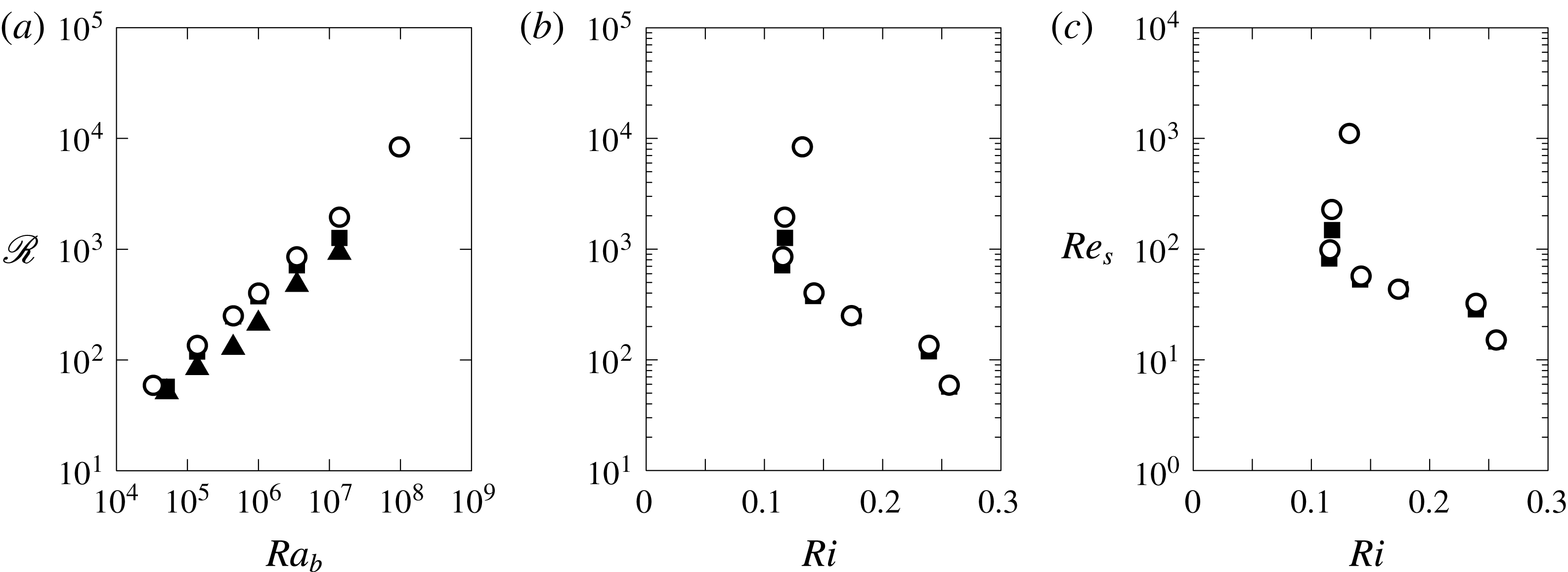
is negative for VC. The length scales defined in (5.1) can also be written in the form of the dimensionless parameters that define scale separations for stratified turbulence:
 $$\begin{eqnarray}\displaystyle \mathit{Ri}\equiv (N^{2}/S^{2})=(l_{c}/l_{o})^{4/3},\quad \mathscr{R}\equiv (l_{o}/\unicode[STIX]{x1D702})^{4/3},\quad \mathit{Re}_{s}\equiv (l_{c}/\unicode[STIX]{x1D702})^{4/3}, & & \displaystyle\end{eqnarray}$$
(cf. Chung & Matheou Reference Chung and Matheou2012) which are the gradient Richardson number, buoyancy Reynolds number and shear Reynolds number, respectively.
Comparison of length scale separations in HVC (▪), HVCws (▴) and bulk of VC (○) using (a)
 $\mathscr{R}$
versus
 $\mathit{Ra}_{b}$
, (b)
 $\mathscr{R}$
versus
 $\mathit{Ri}$
and (c)
 $\mathit{Re}_{s}$
versus
 $\mathit{Ri}$
. The quantities
 $\mathscr{R}$
,
 $\mathit{Ri}$
and
 $\mathit{Re}_{s}$
are defined in (5.2). For HVC without shear,
 $\mathit{Ri}=\text{inf}$
, and these data are therefore not shown in (b) and (c).

Figure 4(a) shows the trends of
 $\mathscr{R}$
versus
 $\mathit{Ra}_{b}$
for the homogeneous cases and for the bulk of VC. Note that for VC, we define
 $L\equiv L_{z}$
the length scale for
 $\mathit{Ra}_{b}$
, since
 $L_{z}$
is the shortest domain length for this set-up. From figure 4(a), the trends of
 $\mathscr{R}$
for the homogeneous cases are comparable to the bulk of VC, suggesting that the choices of
 $N^{2}$
and
 $S$
based on the channel-centre gradients of VC are reasonable. Similarly, the trends of
 $\mathscr{R}$
versus
 $\mathit{Ri}$
in figure 4(b) and
 $\mathit{Re}_{s}$
versus
 $\mathit{Ri}$
in figure 4(c) are also approximately equal. The
 $\mathit{Ri}$
-values are plotted on the abscissae since they are pre-determined input parameters for HVC, whereas both
 $\mathscr{R}$
and
 $\mathit{Re}_{s}$
on the ordinates are responses of HVC. In contrast, all three parameters are the responses of the bulk of VC. The agreement of the magnitudes of (5.1) in figures 4(b) and 4(c) for HVC and bulk of VC indicates that the turbulent quantities in HVC respond in a scale-wise similar manner to the turbulent quantities in the bulk of VC.
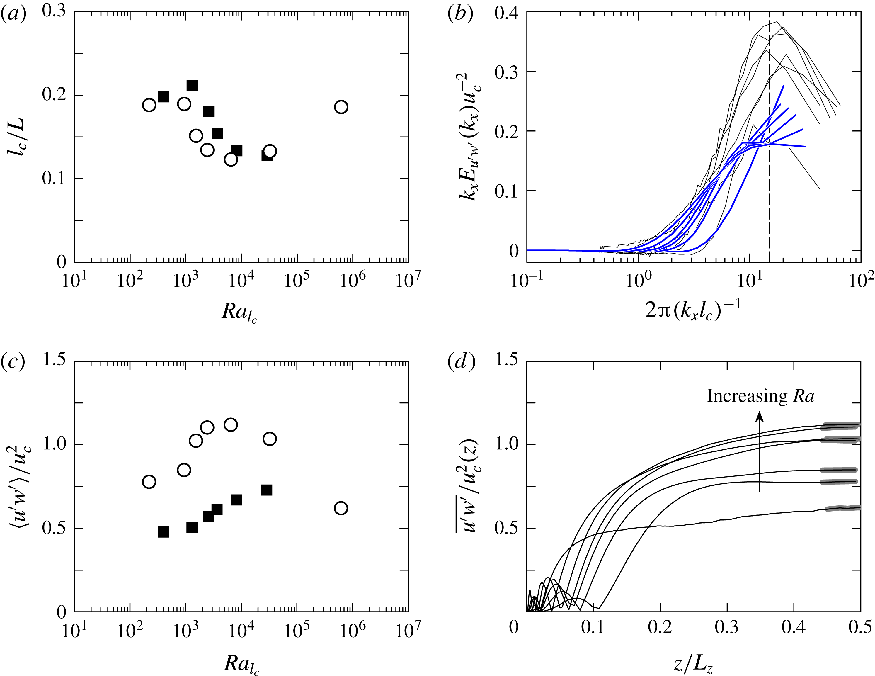
(a) Comparison of the normalised Corrsin length
 $l_{c}/L$
versus
 $\mathit{Ra}_{l_{c}}$
the Rayleigh number based on
 $l_{c}$
, plotted for the bulk of VC (○) and HVC (▪). For VC,
 $L\equiv L_{z}$
and for HVC,
 $L\equiv L_{y}$
. (b) Premultiplied one-dimensional spectra of
 $u^{\prime }w^{\prime }$
normalised by the Corrsin velocity
 $u_{c}$
for the bulk of VC (——) and HVC (—— (blue)). The vertical dashed line indicates the dominant wavelength of
 $\unicode[STIX]{x1D706}_{x,p}\equiv 2\unicode[STIX]{x03C0}k_{x}^{-1}\approx 15l_{c}$
. (c) Ratio of the Reynolds shear stress to
 $u_{c}^{2}$
for the bulk of VC and HVC, where the symbols used are the same as in (a). (d) Similar to (c) for VC but plotted as a function of wall-normal location
 $z/L_{z}$
. The averages of the grey regions in (d) correspond to the values plotted for VC in (c). Note that although the highest
 $\mathit{Ra}$
profile deviates from the overall trend the ratio remains roughly
 ${\sim}O(1)$
.

In figure 5(a), we find that the magnitudes of the normalised Corrsin length scales for HVC and the bulk of VC are in good agreement. To facilitate comparison, we define the Rayleigh number for VC based on
 $l_{c}$
. Noting also that
 $l_{c}$
is normalised by
 $L_{y}$
for HVC, and by
 $L_{z}$
for VC, the good agreement of the trends in figure 5(a) further suggests that
 $L_{y}$
can be considered as an appropriate characteristic length scale for the homogeneous cases, which is consistent with the limiting role of the shorter
 $L_{y}$
dimension discussed in Sekimoto et al. (Reference Sekimoto, Dong and Jiménez2016). In figure 5(b), we compare the one-dimensional premultiplied spectra of
 $u^{\prime }w^{\prime }$
the Reynolds shear stress in the streamwise direction, normalised with
 $u_{c}$
the Corrsin velocity scale. Although the magnitude of the spectra for HVC is reduced owing to the restricted computational domain, both trends from HVC and VC roughly agree when scaled using the Corrsin units. The dominant streamwise wavelength corresponding to the peak in the premultiplied spectra is
 $\unicode[STIX]{x1D706}_{x,p}\equiv 2\unicode[STIX]{x03C0}k_{x}^{-1}\approx 15l_{c}$
for both HVC and VC for the present
 $\mathit{Ra}_{b}$
-range. A more straightforward comparison between the Reynolds shear stress and Corrsin velocity scale is shown in figure 5(c), where we plot the values of
 $\langle u^{\prime }w^{\prime }\rangle /u_{c}^{2}$
versus
 $\mathit{Ra}_{l_{c}}$
for both HVC and bulk of VC. In the case of VC, the values are calculated as the average in the channel centre between
 $0.45\leqslant z/L_{z}\leqslant 0.55$
where the ratio of
 $u^{\prime }w^{\prime }(z)/u_{c}^{2}(z)$
is approximately constant, as shown by the grey shaded lines in figure 5(d). The approximately constant trend of
 $u^{\prime }w^{\prime }(z)/u_{c}^{2}(z)$
close to the channel centre of VC also implies that the Corrsin units are candidate scales for the bulk flow with shear. From both figure 5(c,d), we find that the fractions are both
 ${\sim}O(1)$
, which suggest that
 $u_{c}$
is a reasonable measure of
 $u^{\prime }w^{\prime }$
for the HVC flow, i.e. in support of our earlier assumption in § 3.2 that
 $u^{\prime }w^{\prime }\sim u_{c}^{2}$
.
The results from our analysis of the length scales are encouraging. Although the homogeneous set-ups are idealisations and do not represent the bulk flow of VC, the turbulent scales generated in the homogeneous cases are similar to the turbulent scales generated in the bulk of VC. Thus, keeping this insight in mind, we analyse and compare the scaling relations for VC and the homogeneous set-ups in the next section.
6 Scaling relations in VC and homogeneous VC
In the following, we test several assumptions using the results from the homogeneous cases. This is followed by the scaling of the Nusselt and Reynolds numbers, where we find reasonable agreement between the effective power laws and the expected
 $1/2$
-power laws derived in § 3. Inspired by this insight, we extend our analysis by testing the scaling of
 $\mathit{Nu}$
and
 $\mathit{Re}$
using the turbulent quantities in the bulk of VC.
6.1 Validation of assumptions
In this section we validate several assumptions employed in § 3, namely, the assumptions that
 $\langle u^{\prime }\unicode[STIX]{x1D6E9}^{\prime }\rangle \sim \langle w^{\prime }\unicode[STIX]{x1D6E9}^{\prime }\rangle$
,
 $\unicode[STIX]{x1D6E5}_{b}\sim \unicode[STIX]{x1D6E9}_{rms}$
and
 $u_{b}\sim u_{rms}$
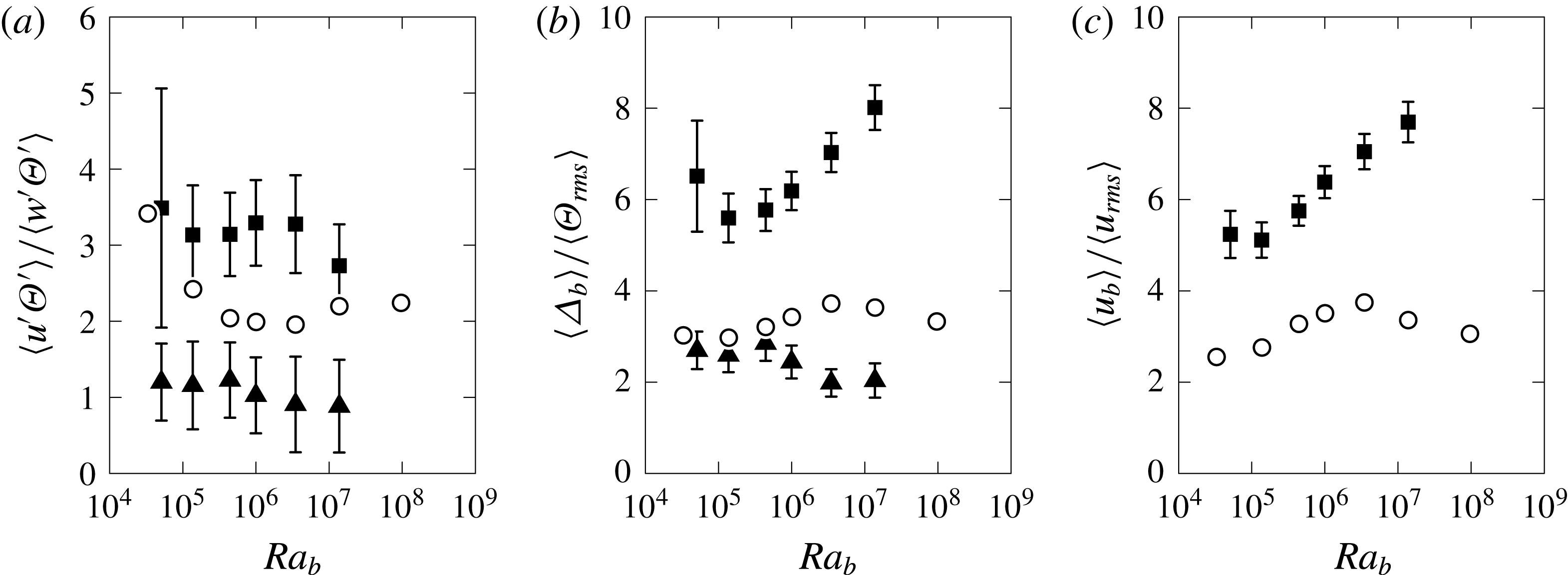
for the homogeneous cases. The three trends are plotted in figure 6 as fractions of their respective means with increasing
 $\mathit{Ra}_{b}$
. The solid square symbols represent the HVC case, solid triangle symbols for HVCws and open circles for VC. In figure 6(a), the trends of
 $\langle u^{\prime }\unicode[STIX]{x1D6E9}^{\prime }\rangle /\langle w^{\prime }\unicode[STIX]{x1D6E9}^{\prime }\rangle$
are approximately constant for the
 $\mathit{Ra}_{b}$
range for both homogeneous set-ups and for VC, which suggest that it is reasonable to assume that
 $\langle u^{\prime }\unicode[STIX]{x1D6E9}^{\prime }\rangle \sim \langle w^{\prime }\unicode[STIX]{x1D6E9}^{\prime }\rangle$
. In contrast, both
 $\langle \unicode[STIX]{x1D6E5}_{b}\rangle /\langle \unicode[STIX]{x1D6E9}_{rms}\rangle$
and
 $\langle u_{b}\rangle /\langle u_{rms}\rangle$
for HVC and HVCws in figure 6(b,c) exhibit weak
 $\mathit{Ra}_{b}$
-trends, suggesting that our scaling assumptions in § 3 may not be completely fulfilled. We reason that these weak
 $\mathit{Ra}_{b}$
-trends contaminate the effective power-law trends in the homogeneous cases resulting in a close-to-
 $1/2$
scaling exponent (shown later in § 6.2) as opposed to a definitive
 $1/2$
-power-law scaling exponent.
Tests for the assumptions in § 3, using the trends of (a)
 $\langle u^{\prime }\unicode[STIX]{x1D6E9}^{\prime }\rangle /\langle w^{\prime }\unicode[STIX]{x1D6E9}^{\prime }\rangle$
versus
 $\mathit{Ra}_{b}$
, (b)
 $\langle \unicode[STIX]{x1D6E5}_{b}\rangle /\langle \unicode[STIX]{x1D6E9}_{rms}\rangle$
versus
 $\mathit{Ra}_{b}$
, and (c)
 $\langle u_{b}\rangle /\langle u_{rms}\rangle$
versus
 $\mathit{Ra}_{b}$
. Cases shown are for HVC (▪), HVCws (▴) and bulk of VC (○). The error bars represent half of the standard deviation from the mean of the fractions.

From figure 6(b), we can further analyse the trends of
 $\langle \unicode[STIX]{x1D6E5}_{b}\rangle /\langle \unicode[STIX]{x1D6E9}_{rms}\rangle$
for both HVC and HVCws to substantiate our numerical approximation employed in our DNS (see § 2.1). We not only require that
 $\unicode[STIX]{x1D6E5}_{b}\sim \unicode[STIX]{x1D6E9}_{rms}$
to satisfy the scaling assumptions in § 3, but also that
 $\unicode[STIX]{x1D6E5}_{b}/\unicode[STIX]{x1D6E9}_{rms}>1$
so that
 $b_{rms}/N^{2}=(\unicode[STIX]{x1D6E5}_{b}/\unicode[STIX]{x1D6E9}_{rms})^{-1}L_{z}<L_{z}$
, which is modestly fulfilled by the trends shown in figure 6(b). We acknowledge that whilst the values of the fractions are not significantly larger than 1, we contend with this limitation by restricting our analyses to only the energetic contributions from the length scales smaller than
 $L_{z}$
, thereby also fulfilling the inequality. To that end, we apply a spectral filter in our calculations of the Nusselt and Reynolds numbers to discard the low-wavenumber (long-wavelength) contributions. In the subsequent sections, the filtered quantities are denoted with a superscript
 $^{\ast }$
, where
 $$\begin{eqnarray}\displaystyle (\cdot )^{\ast }=\int _{k_{3}^{\ast }}^{\infty }E_{(\cdot )}(k_{3})\,\text{d}k_{3}, & & \displaystyle\end{eqnarray}$$
 $k_{3}$
the horizontal wavenumber and
 $2\unicode[STIX]{x03C0}(k_{3}^{\ast })^{-1}=\unicode[STIX]{x1D706}_{3}^{\ast }=0.5L_{z}$
.
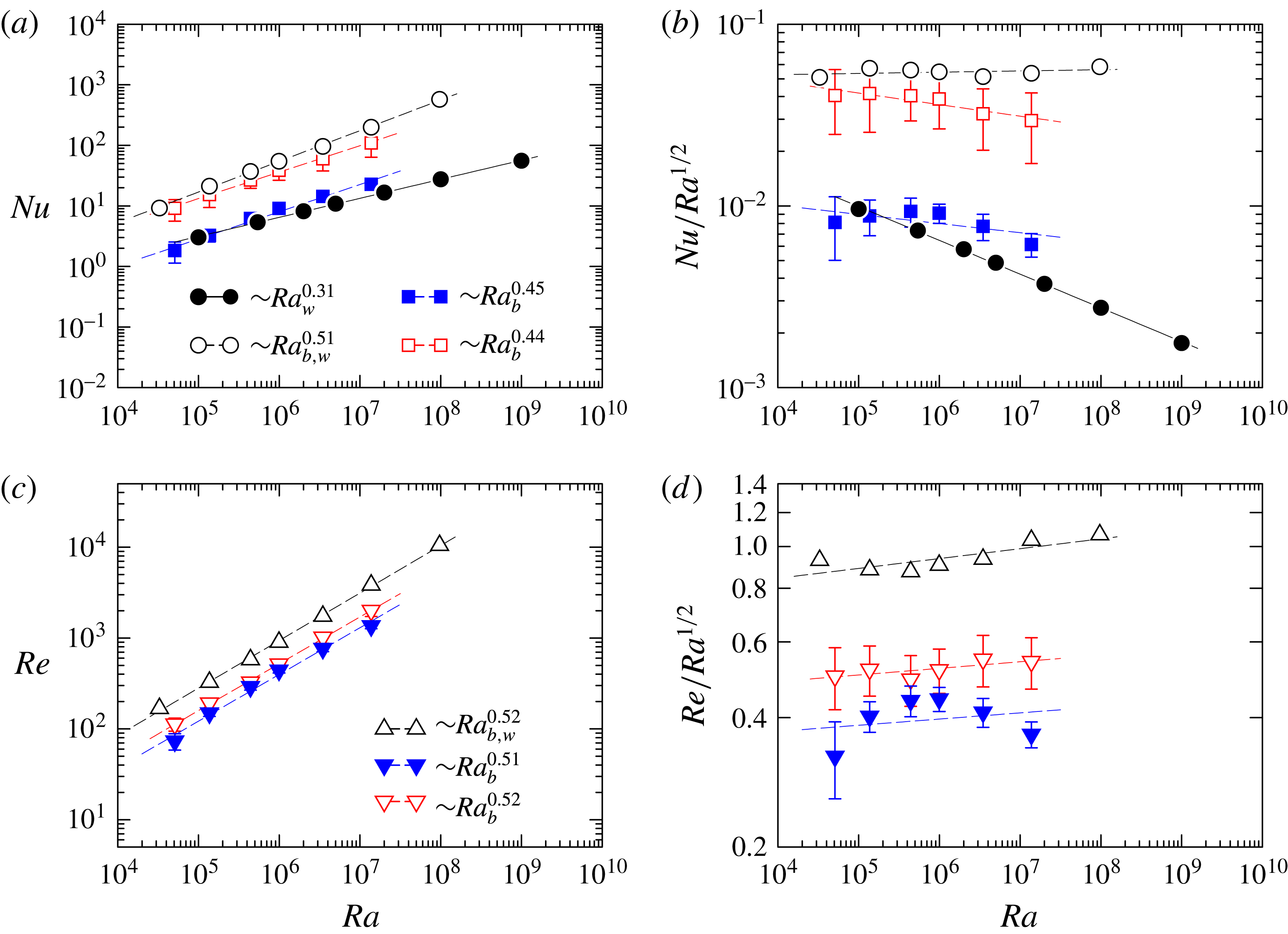
(a) Trends of Nusselt number versus Rayleigh number with slopes that are close to
 $1/2$
for the HVC case with shear (▪ (blue)), without shear (▫ (red)) and bulk of VC (○). The slopes are steeper than the
 ${\sim}\mathit{Ra}_{w}^{0.31}$
trend of the wall-gradient-based Nusselt number for VC (●). (c) Same as in (a), but now reproduced for Reynolds number, again showing slopes that are close to
 $1/2$
for the HVC case with shear (▾ (blue)), without shear (▿ (red)) and bulk of VC (▵). (b,d) Same trends as in (a) and (c) but compensated by the
 $1/2$
-power law for emphasis. Note that the Nusselt and Reynolds numbers for the HVC cases are based on the spectrally filtered small-scale quantities, as defined by (6.1). The error bars represent half of the standard deviation from the time-averaged Nusselt and Reynolds numbers.

6.2 Scaling of
$\mathit{Nu}$
and
$\mathit{Re}$


We begin our scaling analyses by re-plotting the Nusselt number versus the Rayleigh number for VC, where
 $\mathit{Nu}_{w}\equiv JL_{z}/(\unicode[STIX]{x0394}\unicode[STIX]{x1D705})$
and
 $\mathit{Ra}_{w}\equiv g\unicode[STIX]{x1D6FD}\unicode[STIX]{x0394}L_{z}^{3}/(\unicode[STIX]{x1D708}\unicode[STIX]{x1D705})$
, using the DNS data from Ng et al. (Reference Ng, Ooi, Lohse and Chung2015), where
 $(\cdot )_{w}$
denotes dimensionless quantities for VC. Figure 7(a) shows the
 $\mathit{Nu}_{w}$
versus
 $\mathit{Ra}_{w}$
trend (black solid circles). When fitting a single power-law expression,
 $\mathit{Nu}_{w}\sim \mathit{Ra}_{w}^{\unicode[STIX]{x1D6FC}_{w}}$
, a least-squares fit results in
 $\unicode[STIX]{x1D6FC}_{w}\approx 0.31$
, obviously much smaller than the
 $1/2$
-power-law exponent predicted in § 3.
Now, we compare the effective exponent
 $\unicode[STIX]{x1D6FC}_{w}$
to the effective exponents for the two homogeneous cases. We shall consider only the low-wavenumber-filtered Nusselt number, in accordance with our definition in (6.1), and the results of
 $\mathit{Nu}_{b}^{\ast }$
versus
 $\mathit{Ra}_{b}$
are plotted in figure 7(a). With
 $\mathit{Nu}_{b}^{\ast }\sim \mathit{Ra}_{b}^{\unicode[STIX]{x1D6FC}_{h}}$
, the effective scaling exponent for HVC (solid blue squares) is
 $\unicode[STIX]{x1D6FC}_{h}\approx 0.45$
. The corresponding scaling for HVCws, using
 $\mathit{Nu}_{b}^{\ast }\sim \mathit{Ra}_{b}^{\unicode[STIX]{x1D6FC}_{hns}}$
(open red squares) is
 $\unicode[STIX]{x1D6FC}_{hns}\approx 0.44$
. Both
 $\unicode[STIX]{x1D6FC}_{h}$
and
 $\unicode[STIX]{x1D6FC}_{hns}$
are steeper than
 $\unicode[STIX]{x1D6FC}_{w}$
, and are close to the
 $1/2$
-power-law scaling. While not exactly equal to
 $1/2$
, the close-to-
 $1/2$
effective power-law scalings in the homogeneous cases suggest that the homogeneous flow largely behaves in a manner similar to what is expected in the scaling arguments in § 3. The assumptions employed in § 3 may also have a weak influence, which we discuss previously in § 6.1. We accentuate the variations from the
 $1/2$
-power law by plotting the Nusselt number compensated by
 $\mathit{Ra}^{-1/2}$
in figure 7(b), where the non-horizontal trends from our homogeneous cases reflect the deviation from the
 $1/2$
-power-law scaling. Our effective power-law scalings for the homogeneous cases are consistent with similar homogeneous studies on thermal convection but for different configurations, i.e. homogeneous RBC (e.g. Lohse & Toschi Reference Lohse and Toschi2003; Calzavarini et al.
Reference Calzavarini, Lohse, Toschi and Tripiccione2005) and axially homogeneous RBC (e.g. Schmidt et al.
Reference Schmidt, Calzavarini, Lohse, Toschi and Verzicco2012). Thus, it appears that the
 $1/2$
-power-law dependency can be found in homogeneous VC where the thermal convection is quickly determined by the turbulent bulk.
Inspired by the bulk scaling behaviour from the homogeneous cases, we now attempt to apply our understanding to VC. Unlike in RBC where the temperature gradient in the bulk is nominally zero (Sun, Cheung & Xia Reference Sun, Cheung and Xia2008; Zhou et al.
Reference Zhou, Stevens, Sugiyama, Grossmann, Lohse and Xia2010) the temperature gradient in the bulk of VC is not. Therefore, we redefine the Rayleigh and Nusselt numbers for VC based on the quantities in the bulk of VC. Specifically, we define
 $\unicode[STIX]{x1D6E5}_{b}=-L_{z}(\text{d}\overline{\unicode[STIX]{x1D6E9}}/\text{d}z)|_{c}$
the bulk temperature scale in the channel centre of VC. Additionally, since the horizontal heat flux is constant throughout the channel, the definition of
 $J$
for the bulk
 $\mathit{Nu}$
is unchanged. Thus, the bulk quantities for VC can be defined by
 $\mathit{Nu}_{b,w}\equiv \mathit{Nu}_{b}$
and
 $\mathit{Ra}_{b,w}\equiv \mathit{Ra}_{b}$
, and the trend is plotted in figure 7(a) (black open circles). Interestingly, the least-squares fit to the power law
 $\mathit{Nu}_{b,w}\sim \mathit{Ra}_{b,w}^{\unicode[STIX]{x1D6FC}_{b,w}}$
gives
 $\unicode[STIX]{x1D6FC}_{b,w}\approx 0.51$
which is close to
 $1/2$
and of course much larger than the effective exponent
 $\unicode[STIX]{x1D6FC}_{w}\approx 0.31$
discussed earlier. The horizontal trend is also illustrated in the compensated plot of figure 7(b). It appears that the
 $1/2$
-power scaling for bulk-dominated thermal convection may actually exist in all our previous simulations of VC even at low
 $\mathit{Ra}$
, if
 $\unicode[STIX]{x1D6E5}_{b}$
is used instead of
 $\unicode[STIX]{x1D6E5}$
. However, further investigations, such as
 $\mathit{Pr}$
regime studies, may be necessary to determine if this is indeed truly the case.
Moving on to the scaling of the Reynolds numbers, we plot
 $\mathit{Re}_{b}$
versus
 $\mathit{Ra}_{b}$
for the homogeneous cases and for VC in figure 7(c). For VC, we define the velocity scale as the root-mean-square (r.m.s.) of the streamwise velocity fluctuations at the channel centre, i.e.
 $U\equiv u_{rms,w}=(u^{\prime 2})^{1/2}|_{c}$
, and therefore
 $\mathit{Re}_{b,w}\equiv u_{rms,w}L/\unicode[STIX]{x1D708}$
. In figure 7(d), we accentuate the trends by plotting in the
 $1/2$
-power compensated form. For the homogeneous cases, we again compute the low-wavenumber-filtered Reynolds number values, according to (6.1). For HVC, we obtain
 $\mathit{Re}_{b}^{\ast }\sim \mathit{Ra}_{b}^{0.51}$
and for HVCws, we obtain
 $\mathit{Re}_{b}^{\ast }\sim \mathit{Ra}_{b}^{0.52}$
. The effective scaling exponents for the homogeneous cases are still in good agreement with the predictions in § 3. In addition, the exponents from the homogeneous cases are also close to the effective exponent from the bulk of VC, where we obtain
 $\mathit{Re}_{b,w}\sim \mathit{Ra}_{b,w}^{0.52}$
. The present results suggest that, even for VC, by selecting r.m.s.-based parameters to define the Reynolds number, we obtain an effective power law that is consistent with the
 $1/2$
-power-law scaling for bulk-dominated thermal convection. Indeed, our r.m.s.-based scaling results appear to be consistent not only with studies for RBC, (e.g. Emran & Schumacher Reference Emran and Schumacher2008; van Reeuwijk et al.
Reference van Reeuwijk, Jonker and Hanjalić2008) but also for the Rayleigh–Taylor flow, where light fluid is accelerated into heavy fluid (e.g. Celani, Mazzino & Vozella Reference Celani, Mazzino and Vozella2006).
As a final note, the
 $1/2$
effective power-law scaling results in figure 7 for the homogeneous cases are not unexpected results; the homogeneous cases described by (2.5) obey the
 $1/2$
-power scaling arguments for the turbulent bulk-dominated regime as described by Grossmann & Lohse (Reference Grossmann and Lohse2000) (see § 3 above). As such, the homogeneous cases are merely alternative configurations to test the
 $1/2$
-power-law scaling arguments but are not models for the bulk flow of VC.
7 Exponential growth
Homogeneous simulations of RBC have been reported to exhibit unstable and so-called ‘elevator modes’ at low Rayleigh numbers, and are typically represented using exponentially growing values of the Nusselt number, followed by sudden breakdowns (Calzavarini et al. Reference Calzavarini, Lohse, Toschi and Tripiccione2005, Reference Calzavarini, Doering, Gibbon, Lohse, Tanabe and Toschi2006a ). In this section, we examine the solutions of the homogeneous set-up in order to determine whether such exponentially growing solutions also exist, and how the solutions compare to homogeneous RBC. To allow for a comparison between the homogeneous set-up and homogeneous RBC, we restrict our analysis only to the case for HVCws (cf. § 2.2).
We begin our analysis by employing the method of small disturbances (cf. § 2.5 Monin & Yaglom Reference Monin and Yaglom2007) to the linearised equations of (2.5), but without both the terms with shear and the non-periodic term in (2.5c
). That is, we set higher-order fluctuating terms to zero. When made dimensionless using the velocity scale
 $\unicode[STIX]{x1D705}/L$
, temperature scale
 $\unicode[STIX]{x1D6E5}_{b}$
and the length scale
 $L$
, which we represent by the notation
 $(\cdot )^{\prime \prime }$
, the linear equations take the form
 $$\begin{eqnarray}\displaystyle {\displaystyle \frac{\unicode[STIX]{x2202}u_{i}^{\prime \prime }}{\unicode[STIX]{x2202}x_{i}^{\prime \prime }}} & = & \displaystyle 0,\end{eqnarray}$$
 $$\begin{eqnarray}\displaystyle {\displaystyle \frac{\unicode[STIX]{x2202}\unicode[STIX]{x1D6E9}_{i}^{\prime \prime }}{\unicode[STIX]{x2202}t^{\prime \prime }}} & = & \displaystyle {\displaystyle \frac{\unicode[STIX]{x2202}^{2}\unicode[STIX]{x1D6E9}^{\prime \prime }}{\unicode[STIX]{x2202}x_{j}^{\prime \prime 2}}}+u_{3}^{\prime \prime }\end{eqnarray}$$
 $$\begin{eqnarray}\displaystyle {\displaystyle \frac{\unicode[STIX]{x2202}u_{i}^{\prime \prime }}{\unicode[STIX]{x2202}t^{\prime \prime }}} & = & \displaystyle -{\displaystyle \frac{\unicode[STIX]{x2202}p^{\prime \prime }}{\unicode[STIX]{x2202}x_{i}^{\prime \prime }}}+\mathit{Pr}\left({\displaystyle \frac{\unicode[STIX]{x2202}^{2}u_{i}^{\prime \prime }}{\unicode[STIX]{x2202}x_{j}^{\prime \prime 2}}}+\mathit{Ra}_{b}\unicode[STIX]{x1D6E9}^{\prime \prime }\unicode[STIX]{x1D6FF}_{i1}\right).\end{eqnarray}$$
 $$\begin{eqnarray}\displaystyle \unicode[STIX]{x1D703}^{\prime \prime }=\widehat{\unicode[STIX]{x1D703}}\text{e}^{st+\text{i}\boldsymbol{k}\cdot \boldsymbol{x}}+\text{ c.c.},\quad u_{i}^{\prime \prime }=\widehat{u}_{i}\text{e}^{st+\text{i}\boldsymbol{k}\cdot \boldsymbol{x}}+\text{ c.c.}, & & \displaystyle\end{eqnarray}$$
into (7.1a–c
), where
 $\boldsymbol{k}=(k_{1},k_{2},k_{3})$
is the three-dimensional wavenumber. Then, the relation between the complex growth rates
 $s$
and the wavevector
 $\boldsymbol{k}$
can be determined from the eigenvalue problem
 $$\begin{eqnarray}\displaystyle s\widehat{\unicode[STIX]{x1D703}}=-k^{2}\widehat{\unicode[STIX]{x1D703}}+\widehat{u}_{3},\quad s\widehat{u}_{i}=-\mathit{Pr}\,k^{2}\widehat{u}_{i}+\mathit{Ra}_{b}\,\mathit{Pr}\left(-{\displaystyle \frac{k_{1}k_{i}}{k^{2}}}+\unicode[STIX]{x1D6FF}_{i1}\right)\widehat{\unicode[STIX]{x1D703}}, & & \displaystyle\end{eqnarray}$$
where
 $k^{2}\equiv |\boldsymbol{k}|^{2}$
. Equation (7.3) has as solutions four eigenvalues
 $s_{1},\ldots ,s_{4}$
. Out of them
 $$\begin{eqnarray}\displaystyle s_{4,V}=-{\displaystyle \frac{1}{2}}k^{2}(\mathit{Pr}+1)+{\displaystyle \frac{1}{2k^{2}}}\left[(k^{2})^{4}(\mathit{Pr}-1)^{2}-4k_{1}k_{3}k^{2}\mathit{Pr}\mathit{Ra}_{b}\right]^{1/2} & & \displaystyle\end{eqnarray}$$
is the growth rate of interest since the real component of
 $s_{4,V}$
can be positive. Thus, we associate
 $s_{4,V}$
with an unstable mode. The growth rates for HVCws are labelled with a subscript
 $V$
. When the real component of
 $s_{4,V}$
is positive, the imaginary part is always zero, whereas when the real component of
 $s_{4,V}$
is negative, the imaginary part can be either zero or have a finite value. The remaining real component of the three eigenvalues
 $s_{1}$
,
 $s_{2}$
and
 $s_{3}$
are always negative, i.e. corresponding to stable modes. For homogeneous RBC, we label the growth rates with the subscript
 $RB$
. Its largest one, which is similarly associated with an unstable mode, takes the form
 $$\begin{eqnarray}\displaystyle s_{4,RB}=-{\displaystyle \frac{1}{2}}k^{2}(\mathit{Pr}+1)+{\displaystyle \frac{1}{2k^{2}}}\left[(k^{2})^{4}(\mathit{Pr}-1)^{2}+4\left(k_{2}^{2}+k_{3}^{2}\right)k^{2}\mathit{Pr}\mathit{Ra}_{b}\right]^{1/2}, & & \displaystyle\end{eqnarray}$$
(cf. Calzavarini et al.
Reference Calzavarini, Lohse, Toschi and Tripiccione2005, Reference Calzavarini, Doering, Gibbon, Lohse, Tanabe and Toschi2006a
). The imaginary component of
 $s_{4,RB}$
is always zero. Similar to HVCws, the remaining three eigenvalues for homogeneous RBC other than (7.5) are always negative. In addition, there are no zero-mode cases in both HVCws and homogeneous RBC since they only occur when
 $\boldsymbol{k}=(0,0,0)$
which corresponds to an unbounded infinite system (Schmidt et al.
Reference Schmidt, Calzavarini, Lohse, Toschi and Verzicco2012). If the solutions of homogeneous RBC are assumed to be independent of
 $x_{1}$
, i.e.
 $k_{1}=0$
, equation (7.5) simplifies to equation (9) of Calzavarini et al. (Reference Calzavarini, Doering, Gibbon, Lohse, Tanabe and Toschi2006a
) for which
 $s_{4,RB}>0$
for
 $\mathit{Ra}_{b}>(k_{2}^{2}+k_{3}^{2})^{2}$
.
Isosurfaces of the marginally stable modes, which have
 $s_{4}=0$
for (a) HVCws and (b) homogeneous RBC at
 $\mathit{Ra}_{b}=2\times 10^{4}$
and
 $\mathit{Pr}=0.709$
. Inside these isosurfaces, the eigenvalues are positive (labelled ● (red)), corresponding to unstable modes. The number of unstable modes thus corresponds to the number of solid red markers enclosed within the isosurface: 2 for HVCws and 16 for homogeneous RBC (in the rotated view (b), only 14 are visible). Outside these isosurfaces, the eigenvalues are negative (labelled ○ (red)), corresponding to stable modes. Thanks to symmetry, the isosurface for
 $k_{2}>0$
do not need to be shown. The isosurfaces are oriented such that
 $k_{1}$
is associated with the physical space variable
 $x_{1}$
, which is opposing gravity. The heat flux is in
 $x_{3}$
-direction in (a) and in
 $x_{1}$
-direction in (b). In (a), the isosurfaces shows a directional dependence in the (
 $k_{2}$
,
 $k_{3}$
) plane, in contrast to (b).

A convenient way to interpret the stability of the modes corresponding to
 $s_{4}$
is to visualise the surfaces of marginally stable modes which have
 $s_{4}=0$
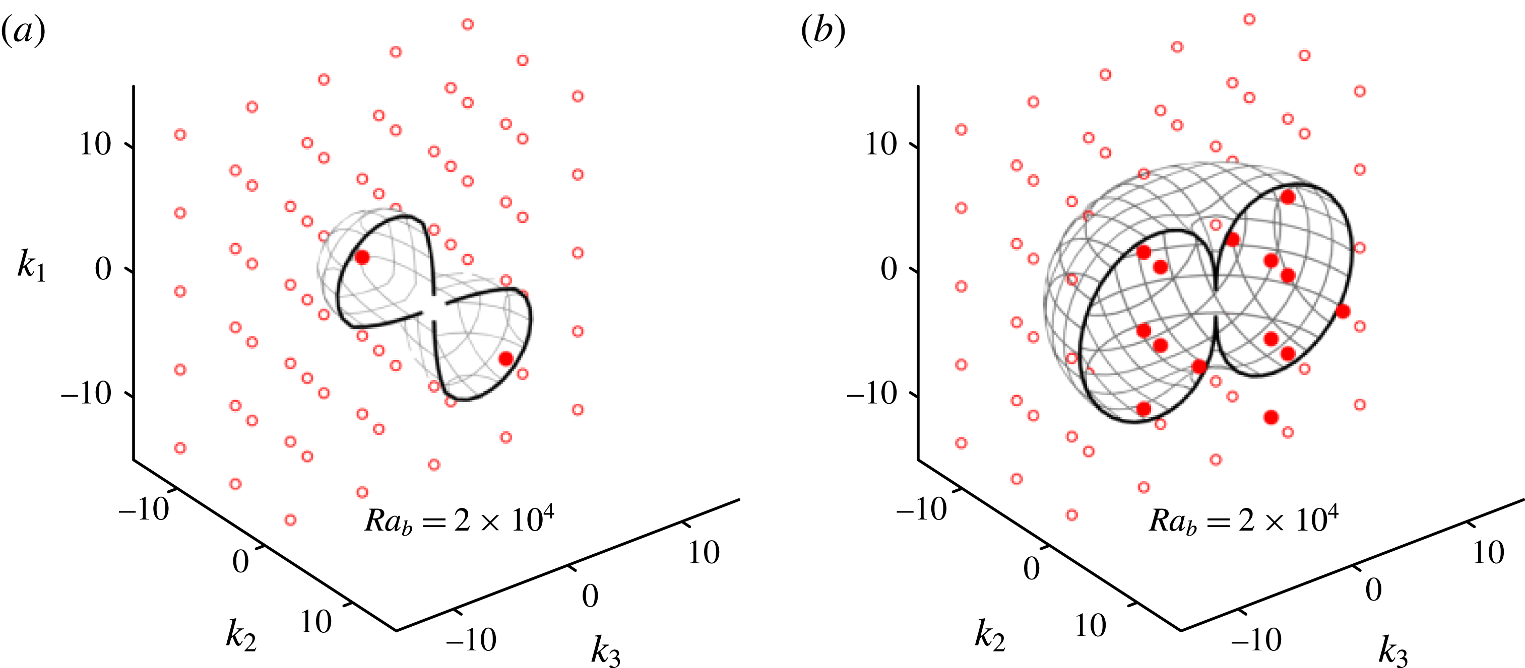
. These isosurfaces are plotted in three-dimensional wavenumber space in figure 8 for both HVCws and homogeneous RBC at
 $\mathit{Ra}_{b}=2\times 10^{4}$
and
 $\mathit{Pr}=0.709$
. A low
 $\mathit{Ra}_{b}$
is chosen for both configurations in order to relate the unstable modes to the behaviour of exponential solutions of
 $\mathit{Nu}_{b}$
that are known to exist in homogeneous RBC (Calzavarini et al.
Reference Calzavarini, Lohse, Toschi and Tripiccione2005, Reference Calzavarini, Doering, Gibbon, Lohse, Tanabe and Toschi2006a
). In figure 8, only half of the isosurfaces need to be shown thanks to symmetry: for HVCws (figure 8
a), only the region
 $k_{2}<0$
is shown since the region is plane symmetrical at
 $k_{2}=0$
; for homogeneous RBC (figure 8
b), only the region
 $k_{2}<0$
is shown since the region is axisymmetric about
 $\boldsymbol{k}=(k_{1},0,0)$
. The axisymmetric nature of the isosurface
 $s_{4,RB}=0$
reflects the invariance of homogeneous RBC towards rotation in the horizontal
 $x_{2}x_{3}$
-plane (Calzavarini et al.
Reference Calzavarini, Doering, Gibbon, Lohse, Tanabe and Toschi2006a
; Schmidt et al.
Reference Schmidt, Calzavarini, Lohse, Toschi and Verzicco2012). In contrast, the isosurface of
 $s_{4,V}=0$
shows directional dependence in HVCws. The red markers represent the
 $\boldsymbol{k}$
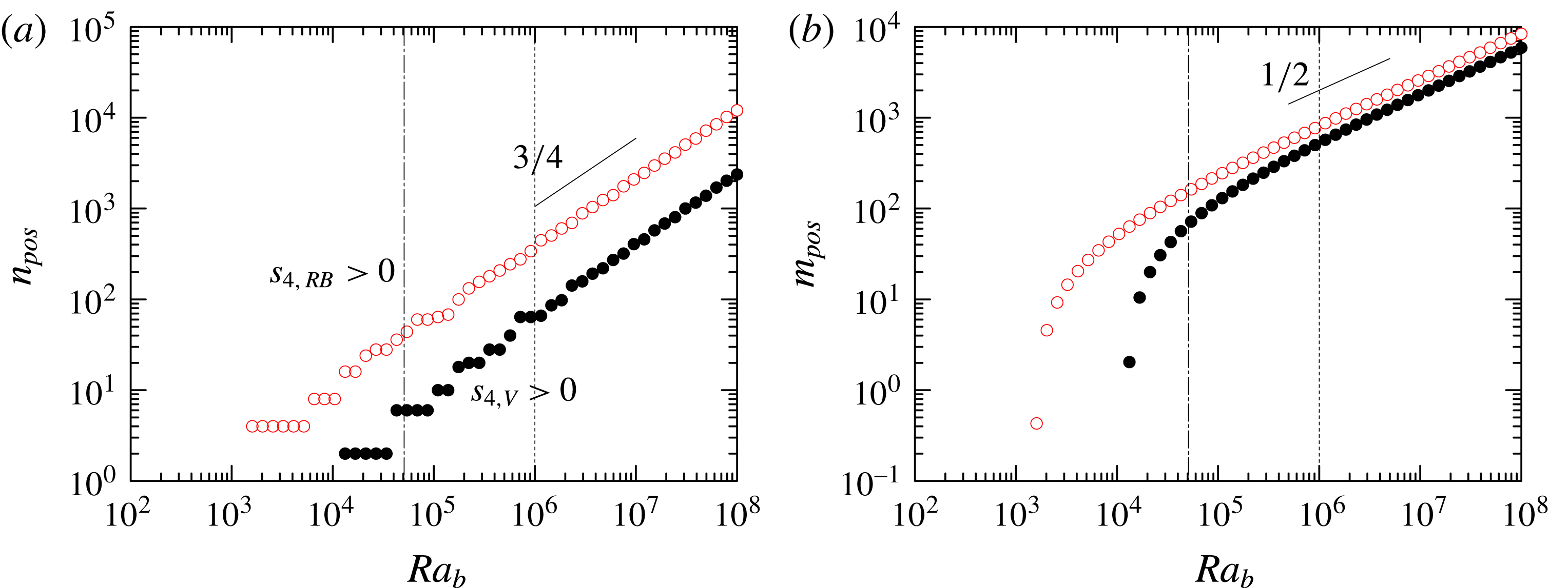
-locations of eigenvalues and any solid red markers enclosed within the isosurface represent positive eigenvalues associated with unstable modes. In figure 8, there are two unstable modes in HVCws compared to 16 unstable modes in homogeneous RBC. Varying
 $\mathit{Ra}_{b}$
for both configurations does not change the shape of the isosurface and merely scales the sizes of the stability regions. Thus, increasing
 $\mathit{Ra}_{b}$
will result in a larger region which encompasses more unstable modes. Since the shapes of the stability regions are unchanged with
 $\mathit{Ra}_{b}$
, it is immediately apparent that the number of positive eigenvalues for homogeneous RBC is larger compared to HVCws at any given
 $\mathit{Ra}_{b}$
. This suggests that at any given
 $\mathit{Ra}_{b}$
, the solutions for homogeneous RBC are exposed to more interactions between unstable modes as compared to the solutions for HVCws. In § 8, we will compare the results of our DNS of HVCws and homogeneous RBC at matched
 $\mathit{Ra}_{b}$
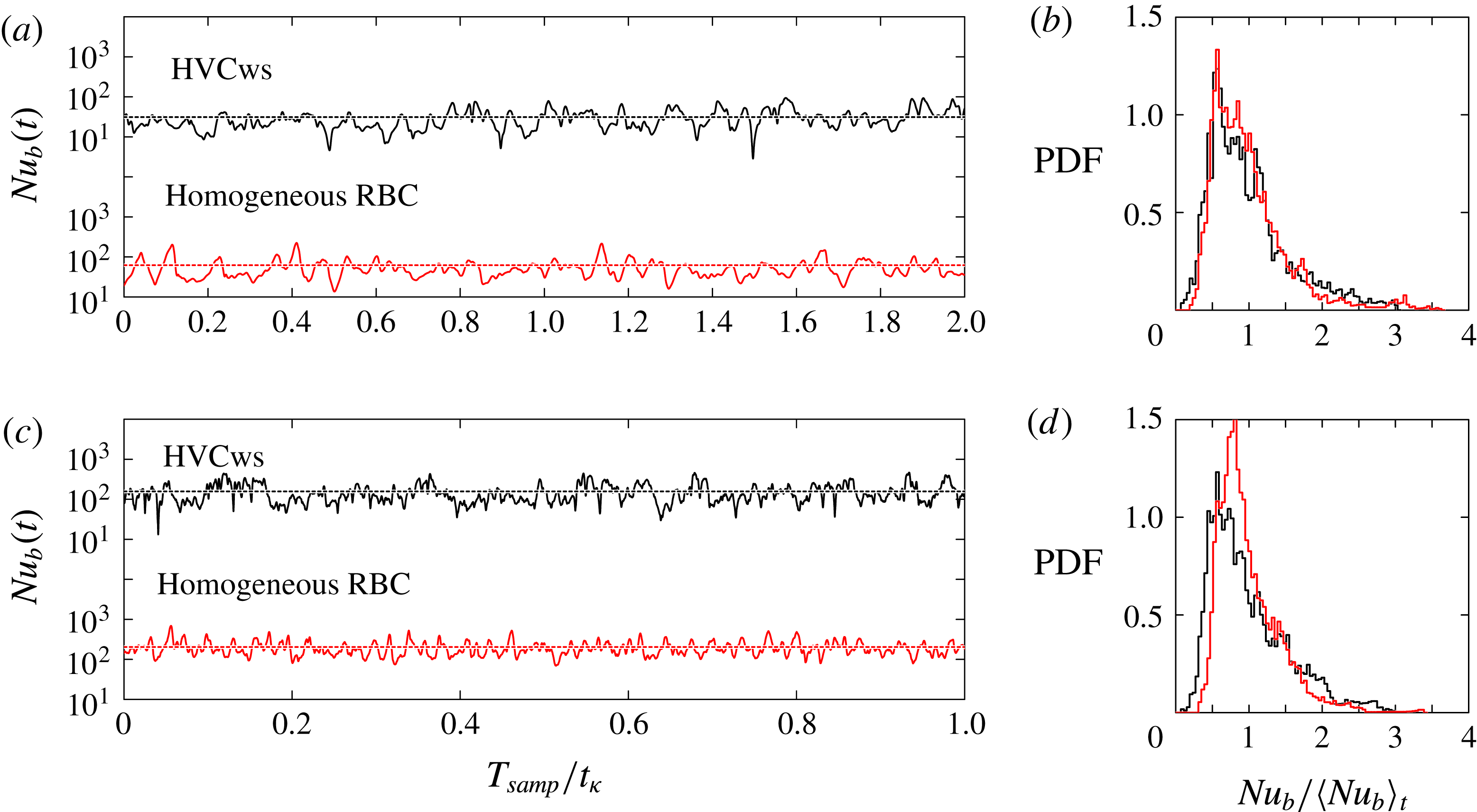
. We find that the increased interactions between unstable modes in homogeneous RBC correlate with increased unsteadiness in the time evolution of
 $\mathit{Nu}_{b}(t)$
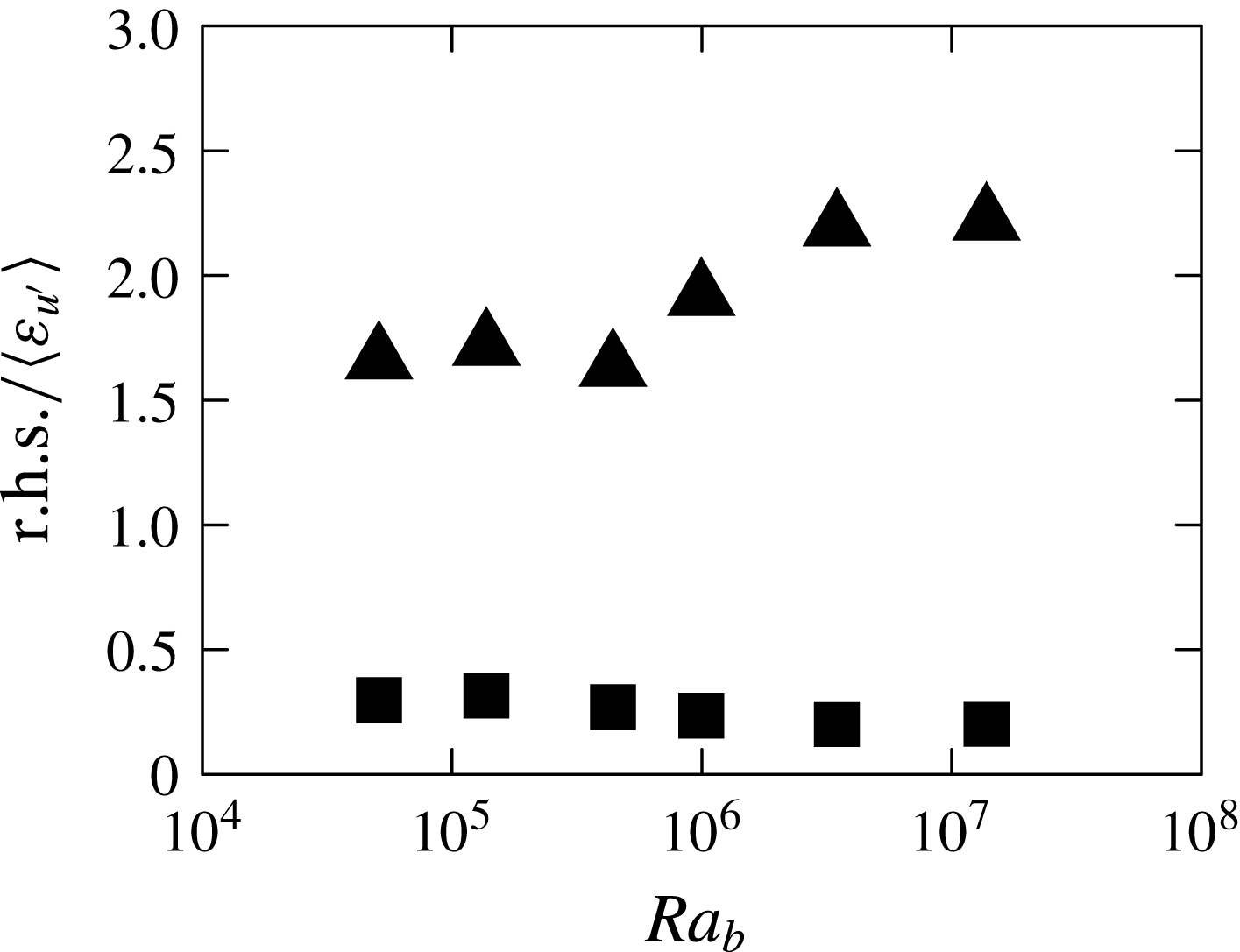
as compared to HVCws.
(a) Count of unstable modes
 $n_{pos}$
using (7.4) for HVCws (●) and (7.5) for homogeneous RBC (○). (b) Largest magnitude of unstable modes
 $m_{pos}$
; each point corresponds to the most unstable mode. In (a), both trends grow as
 $\mathit{Ra}_{b}^{3/4}$
and at matched
 $\mathit{Ra}_{b}$
,
 $n_{pos,RB}>n_{pos,V}$
. In (b), the largest magnitudes of the unstable modes vary as
 $\mathit{Ra}_{b}^{1/2}$
. The vertical lines represent
 $\mathit{Ra}_{b}\simeq 5\times 10^{4}$
(–
 $\cdot$
–
 $\cdot$
) and
 $\mathit{Ra}_{b}\simeq 1\times 10^{6}$
(
 $\cdots \cdots$
). It can be seen that HVCws has fewer numbers of less unstable modes whereas homogeneous RBC has larger numbers of more unstable modes.

To better describe the trend of the unstable modes, the modes for HVCws and homogeneous RBC are quantified for
 $\mathit{Ra}_{b}=10^{3}$
–
 $10^{8}$
by considering the number of positive modes (denoted by
 $n_{pos}$
) for a range of wavenumbers
 $\boldsymbol{k}=2\unicode[STIX]{x03C0}(n_{1},n_{2},n_{3})$
where
 $(n_{1},n_{2},n_{3})$
are the positive- and negative-integer wavenumbers (Calzavarini et al.
Reference Calzavarini, Toschi, Lohse, Tripiccione, Doering, Gibbon and Tanabe2006b
). The trend is plotted in figure 9(a), where black markers represent
 $n_{pos,V}$
and red markers represent
 $n_{pos,RB}$
. From the figure, we find that
 $n_{pos,RB}$
is always larger than
 $n_{pos,V}$
, which is consistent with the number of unstable modes counted at matched
 $\mathit{Ra}_{b}$
for the two configurations of figure 8. This suggests that the solutions for homogeneous RBC will always be more unsteady at all
 $\mathit{Ra}_{b}$
compared to HVCws. We note that both
 $n_{pos}$
vary as
 $\mathit{Ra}_{b}^{3/4}$
at high
 $\mathit{Ra}_{b}$
. Apart from the positive unstable modes, there exist sets of stable modes (which have
 $s_{4}<0$
) in the range of
 $\mathit{Ra}_{b}$
, not shown in figure 9(a). To gain further insight into the stability of the two configurations, the dominance of the most unstable mode at matched
 $\mathit{Ra}_{b}$
is compared in figure 9(b) where we plot the magnitudes of the largest positive real component of
 $s_{4}$
(denoted by
 $m_{pos}$
) in the same
 $\mathit{Ra}_{b}$
range over all wavenumbers. From the figure, we observe that
 $m_{pos}$
for homogeneous RBC is always larger than that of HVCws (both trends vary as
 $\mathit{Ra}^{1/2}$
at high
 $\mathit{Ra}_{b}$
). Thus, from a direct comparison of the trends in figure 9, it could be inferred that the relatively more unsteady solutions for homogeneous RBC (due to higher
 $n_{pos}$
) will present at a larger magnitude on average (due to higher
 $m_{pos}$
) as compared to HVCws. In § 8, we show that the trends from DNS of homogeneous RBC exhibit a higher level of unsteadiness about a larger mean, which is consistent with the observations from the analyses above.
8 Comparison to DNS
 $\mathit{Nu}_{b}(t)$
for HVCws (—— (black)) and homogeneous RBC (—— (red)) for (a)
 $\mathit{Ra}_{b}\simeq 5\times 10^{4}$
and (c)
 $\mathit{Ra}_{b}\simeq 1\times 10^{6}$
at
 $\mathit{Pr}=0.709$
. (
 $b$
,
 $d$
) The corresponding probability density functions (PDFs) of
 $\mathit{Nu}_{b}(t)$
normalised by the time-averaged
 $\mathit{Nu}_{b}$
, indicated by the dotted lines in (a) and (c). At lower
 $\mathit{Ra}_{b}$
in (b), the PDFs for both configurations are positively skewed, which suggests the presence of elevator modes (Calzavarini et al.
Reference Calzavarini, Lohse, Toschi and Tripiccione2005). At higher
 $\mathit{Ra}_{b}$
in (d), the PDFs for both configurations are less skewed, suggesting that the solutions are subjected to a stabilising mechanism.

To further illustrate the results of § 7, we compare the instantaneous Nusselt numbers for HVCws and for homogeneous RBC, and for two relatively low Rayleigh numbers:
 $\mathit{Ra}_{b}\simeq 5\times 10^{4}$
and
 $1\times 10^{6}$
. Both
 $\mathit{Ra}_{b}$
-values are indicated respectively by the dot-dashed and dotted lines in figure 9. For homogeneous RBC, we employ the same box size as that for HVCws, i.e.
 $L_{x}=4L_{y}=2L_{z}$
, and the simulations are resolved up to at least
 $k_{\mathit{max}}\unicode[STIX]{x1D702}\approx 2.71$
. The simulation parameters for HVCws have been described earlier in § 4. We also define the Nusselt number for homogeneous RBC similar to (3.1b
), i.e.
 $\mathit{Nu}_{b}\equiv JL/(\unicode[STIX]{x1D6E5}_{b}\unicode[STIX]{x1D705})$
, but with
 $J\equiv -\unicode[STIX]{x1D705}\unicode[STIX]{x1D6E5}_{b}/L+\langle u^{\prime }\unicode[STIX]{x1D6E9}^{\prime }\rangle$
the vertical heat flux and
 $L\equiv L_{x}$
.
The instantaneous values of
 $\mathit{Nu}_{b}(t)$
are plotted in figure 10(a) for
 $\mathit{Ra}_{b}\simeq 5\times 10^{4}$
and in figure 10(c) for
 $\mathit{Ra}_{b}\simeq 1\times 10^{6}$
. The corresponding probability distribution functions (PDFs) are shown in figure 10(b,d). From the PDFs, the behaviours of
 $\mathit{Nu}_{b}(t)$
of both HVCws and homogeneous RBC appear qualitatively similar at matched
 $\mathit{Ra}_{b}$
. Whilst all PDFs at both lower and higher
 $\mathit{Ra}_{b}$
appear skewed, both PDFs at the lower-
 $\mathit{Ra}_{b}$
value are relatively more positively skewed, which is consistent with the exponentially growing notion of elevator modes at low
 $\mathit{Ra}_{b}$
and is similar to previously reported PDFs of the time evolution of
 $\mathit{Nu}_{b}(t)$
(see for example figure 7(a) in Calzavarini et al.
Reference Calzavarini, Lohse, Toschi and Tripiccione2005). The change from a skewed distribution at lower
 $\mathit{Ra}_{b}$
to a relatively even distribution at higher
 $\mathit{Ra}_{b}$
suggests a stabilising mechanism that can be attributed to the presence and interactions of a larger number of unstable modes at higher
 $\mathit{Ra}_{b}$
, as suggested by Calzavarini et al. (Reference Calzavarini, Doering, Gibbon, Lohse, Tanabe and Toschi2006a
) and Schmidt et al. (Reference Schmidt, Calzavarini, Lohse, Toschi and Verzicco2012).
When comparing the time-averaged values of
 $\mathit{Nu}_{b}(t)$
for HVCws and homogeneous RBC, we find that the
 $\mathit{Nu}_{b}$
is on average larger for homogeneous RBC than for HVCws (figure 10
a,c). These trends agree with the presence of larger numbers of larger unstable modes in homogeneous RBC compared to HVCws, as discussed previously in § 7.
9 Conclusions
Using a series of DNS of homogeneous vertical natural configuration (HVC – with shear, HVCws – without shear) for
 $\mathit{Ra}_{b}$
ranging between
 $10^{5}$
and
 $10^{9}$
and a
 $\mathit{Pr}$
value of 0.709, we find that the Nusselt and Reynolds numbers exhibit close to
 $\mathit{Nu}_{b}\sim \mathit{Ra}_{b}^{1/2}$
and
 $\mathit{Re}_{b}\sim \mathit{Ra}_{b}^{1/2}$
scaling (figure 7), which are consistent with the scaling laws predicted for turbulent bulk-dominated thermal convection at high
 $\mathit{Ra}$
(Kraichnan Reference Kraichnan1962; Grossmann & Lohse Reference Grossmann and Lohse2000). The present
 $1/2$
-power-law scalings are not only consistent with results from previous studies on homogeneous thermal convection, but can also be found in VC when bulk quantities are employed in the definitions of the Nusselt, Reynolds and Rayleigh numbers.
These
 $1/2$
-power-law scaling results for the homogeneous set-ups follow in the wake of the scaling arguments for the turbulent bulk flow. In § 3, we show that both homogeneous set-ups are expected to follow the
 $1/2$
-power-law scalings for both Nusselt and Reynolds numbers, consistent with the spirit of the original derivation in Grossmann & Lohse (Reference Grossmann and Lohse2000). However, in contrast to homogeneous RBC for which the
 $1/2$
-power law can be conveniently derived (as has been shown in Lohse & Toschi Reference Lohse and Toschi2003), the
 $1/2$
-power law in the homogeneous set-up for VC is contingent on several necessary assumptions: the most important assumption being that the vertical turbulent heat flux scales with the horizontal turbulent heat flux and is
 $\mathit{Ra}_{b}$
-independent. We show that the
 $\mathit{Ra}_{b}$
-independence not only holds true for the homogeneous cases investigated, but also in the bulk region of VC (figure 6). Other assumptions, whilst exhibiting slight
 $\mathit{Ra}_{b}$
trends, appear to minimally affect the
 $1/2$
-power-law scaling result.
Although HVC is reminiscent of the bulk of the wall-bounded counterpart (both exhibiting a mean temperature gradient and mean shear), we emphasise that both HVC and HVCws are merely idealisations of the turbulent bulk flow of vertical natural convection. More importantly, the homogeneous cases rightfully capture the orthogonal action of the turbulent vertical convective heat flux and the horizontal heat flux. In addition, the governing equations for the homogeneous cases obey the original scaling arguments in Grossmann & Lohse (Reference Grossmann and Lohse2000) and Lohse & Toschi (Reference Lohse and Toschi2003) (i.e. when the contributions of the dissipation in the boundary layers are minimal).
Focusing now on the solutions for HVCws, from stability analysis, we find that the flow is direction dependent whereas homogeneous RBC is invariant in the vertical direction (figure 8). In addition, solutions for HVCws are found to be always influenced by fewer numbers of less unstable modes as compared to homogeneous RBC, which are always influenced by larger numbers of more unstable modes relative to HVCws (figure 9). At low to moderate
 $\mathit{Ra}_{b}$
, we observe unsteadiness in the solutions (figure 10), similar to the elevator modes previously reported for homogeneous RBC (Calzavarini et al.
Reference Calzavarini, Lohse, Toschi and Tripiccione2005, Reference Calzavarini, Doering, Gibbon, Lohse, Tanabe and Toschi2006a
) and axially homogeneous RBC (Schmidt et al.
Reference Schmidt, Calzavarini, Lohse, Toschi and Verzicco2012). In spite of the unsteadiness, results from the DNS appear robust and exhibit close to the
 $\mathit{Ra}_{b}^{1/2}$
power-law scalings for both Nusselt and Reynolds numbers.
The results from the present work suggest that the asymptotic ultimate
 $1/2$
-power-law scaling can also be found in VC in both the homogeneous cases and in the bulk region of VC. However, the
 $1/2$
-power-law scaling relies on additional assumptions which reasonably agree with the present DNS, but may require further validation in different Rayleigh and Prandtl number regimes.
Premultiplied one-dimensional spectra of
 $u^{\prime }u^{\prime }$
(a,d) in the
 $x$
-direction, (b,e) in the
 $y$
-direction, and (c,f) in the
 $z$
-direction. In (a–c), the streamwise domain is varied where
 $L_{x}=4L_{y}=2L_{z}$
(solid black line, used in our study),
 $L_{x}=6L_{y}=3L_{z}$
(dashed black line) and
 $L_{x}=8L_{y}=4L_{z}$
(dot-dashed black line). In (d–f), the spanwise domain is varied where
 $L_{x}=2L_{y}=2L_{z}$
(dashed blue line) and
 $L_{x}=L_{y}=2L_{z}$
(dot-dashed blue line).

Acknowledgements
This work was supported by the resources from the National Computational Infrastructure (NCI) National Facility in Canberra, Australia, which is supported by the Australian Government, and the Pawsey Supercomputing Centre, which is funded by the Australian Government and the Government of Western Australia. D.L. acknowledges support from FOM via the programme ‘Towards ultimate turbulence’.
Appendix A. Sensitivity of box dimensions on homogeneous simulations
Here, we provide an analysis on the sensitivity of the box dimensions for the HVC set-up. We will make use of the one-dimensional energy spectrum of streamwise velocity
 $u$
, which we define as
 $E_{u^{\prime }u^{\prime }}(k_{i})$
, where
 $(u^{\prime })^{2}=2\int _{0}^{\infty }E_{u^{\prime }u^{\prime }}\,\text{d}k_{i}$
,
 $k_{i}$
is the wavenumber in the
 $i$
th direction,
 $\unicode[STIX]{x1D706}_{i}=2\unicode[STIX]{x03C0}k_{i}^{-1}$
is the corresponding wavelength and
 $i=1,2$
or
 $3$
. In addition, the spectra is plotted in premultiplied form, which provides an intuitive representation on a logarithmic plot since the area under the curve of a premultiplied spectrum visually represents the distribution of energy that reside at the corresponding wavelength. The simulation parameters are set such that we match the values of
 $\mathit{Ra}_{b}$
(
 $=10^{5}$
) and
 $\mathit{Re}_{y}\equiv SL_{y}^{2}/\unicode[STIX]{x1D708}$
(
 ${\approx}640$
), which is the box-width Reynolds number (Sekimoto et al.
Reference Sekimoto, Dong and Jiménez2016). The results are shown in figure 11: in (a–c),
 $L_{x}$
is varied while holding
 $L_{y}$
and
 $L_{z}$
fixed; in (d–f),
 $L_{y}$
is varied while holding
 $L_{x}$
and
 $L_{z}$
fixed.
In figure 11(a–c), the spectra collapses when the spanwise domain length
 $L_{y}$
is used to scale the abscissae, suggesting that the limiting domain
 $L_{y}$
is indeed the characteristic length scale, in agreement with the results of Sekimoto et al. (Reference Sekimoto, Dong and Jiménez2016), and is a suitable choice to define
 $\mathit{Ra}_{b}$
. In addition, any increase of the streamwise domain length does little to close the spectra at the longest wavelengths, which suggest that the energetic wavelengths grow to fill the size of the boxes. A similar behaviour is observed in figure 11(d–f), where
 $L_{y}$
is varied while
 $L_{x}$
and
 $L_{z}$
are fixed. The latter result indicate that the dynamics of the flow remain sensitive to the box size. As a compromise between computational cost and resolving the large scales in our flow, in our study, we select
 $L_{x}=4L_{y}=2L_{z}$
.
Appendix B. Comparison of
$\langle \unicode[STIX]{x1D700}_{u^{\prime }}\rangle$
with (3.3a
) and (3.9a
)

To evaluate the modelled expressions of
 $\langle \unicode[STIX]{x1D700}_{u^{\prime }}\rangle$
, i.e. the right-hand side of (3.3a
) and the right-hand side of (3.9a
), we show the trend of the ratios with increasing
 $\mathit{Ra}_{b}$
in figure 12. Both trends exhibit weak reliance on
 $\mathit{Ra}_{b}$
, albeit slightly more pronounced for the less realistic HVCws set-up, which suggest that the models and underlying assumptions for (3.3a
) and (3.9a
) can modestly predict the average kinetic dissipation rate, at least for the present
 $\mathit{Ra}_{b}$
-range and
 $\mathit{Pr}$
-value.
Ratio of right-hand side of (3.3a
) to
 $\langle \unicode[STIX]{x1D700}_{u^{\prime }}\rangle$
for HVC (solid squares) and right-hand side of (3.9a
) to
 $\langle \unicode[STIX]{x1D700}_{u^{\prime }}\rangle$
for HVCws (solid triangles).
 $\langle \unicode[STIX]{x1D700}_{u^{\prime }}\rangle$
is computed from the gradient of the velocity fluctuations from the DNS.