1 Introduction
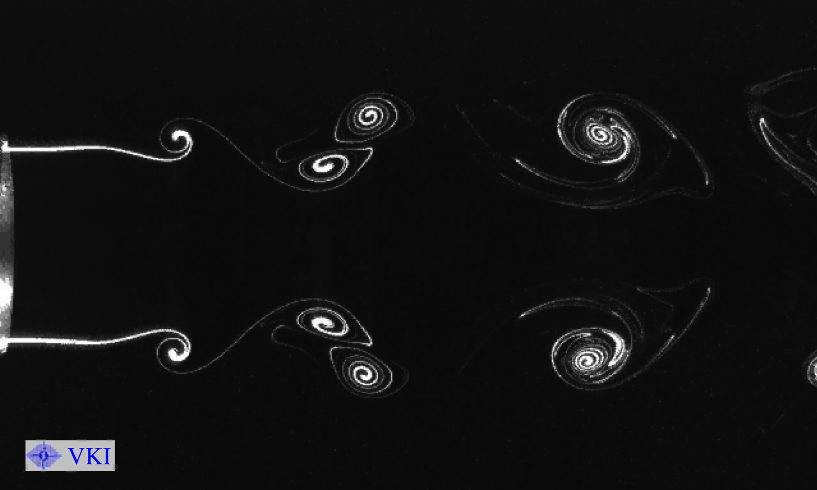
When the shear layer of a jet is subjected to low-level forcing at the nozzle, perturbations within a band of unstable frequencies are amplified as they travel downstream (Michalke Reference Michalke1971). When the perturbation amplitude reaches nonlinear levels, the shear layer rolls up into vortices. In the case of laminar jets, forced axisymmetrically at a single frequency, a regular street of ring vortices is formed, where the passage frequency of vortices is controlled by the nozzle forcing. It has long been observed that such vortices may, in certain parameter regimes, spontaneously undergo regular pairing: two neighbouring vortices then merge into one, such that a new vortex street is formed, with a periodicity that corresponds to the subharmonic of the applied forcing frequency. This scenario is illustrated in figure 1, which shows a flow visualisation from the experiments by Schram (Reference Schram2003). The first systematic studies of the pairing scenario have been conducted by Hussain & Zaman (Reference Hussain and Zaman1980) and Zaman & Hussain (Reference Zaman and Hussain1980). While the merging of two vortices is clearly a nonlinear process, it remains to be clarified to what extent the occurrence of regular vortex pairing is governed by linear mechanisms, and how such linear dynamics may be properly formalised.
Experimental visualisation of pairing in a jet, snapshot of a movie by Schram (Reference Schram2003).

Numerous past studies have sought to explain the pairing phenomenon by investigating the consistency of the paired flow state itself. Monkewitz (Reference Monkewitz1988) developed a theoretical framework based on weakly nonlinear interaction between the forced fundamental instability wave and its subharmonic. His formalism leads to a phase-relation criterion for subharmonic resonance, which has subsequently been validated experimentally by Husain & Hussain (Reference Husain and Hussain1989), Raman & Rice (Reference Raman and Rice1991), Paschereit, Wygnanski & Fiedler (Reference Paschereit, Wygnanski and Fiedler1995) and others.
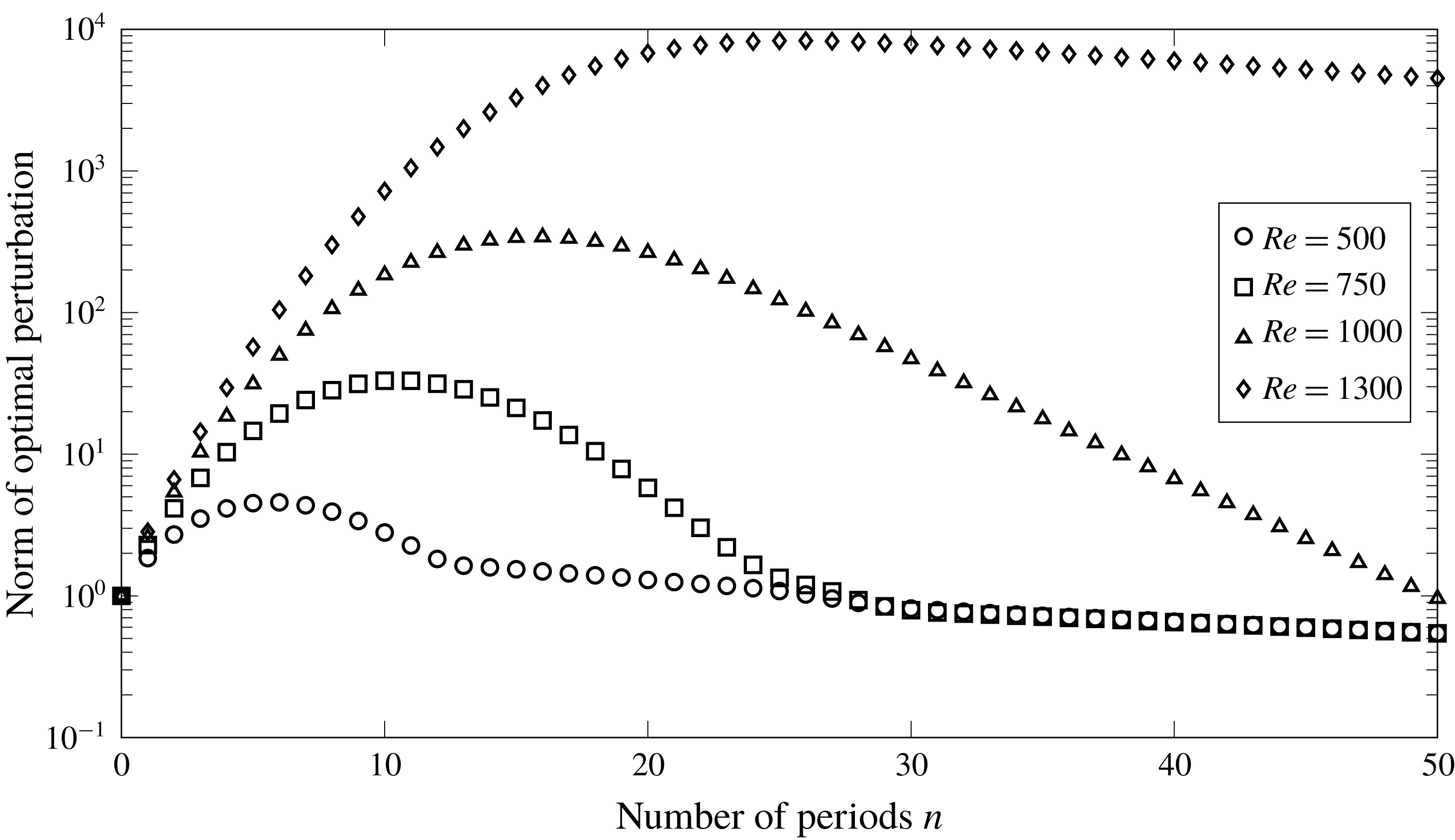
A different approach consists in considering the bifurcation process from a harmonic unpaired to a subharmonic paired state. This viewpoint leads to the question as to whether an array of vortices convecting at the imposed forcing frequency is unstable with respect to subharmonic perturbations. In forced jets, vortex pairing occurs as a self-sustained process, and the pairing location is stationary in a spatially non-periodic flow. Therefore, the appropriate framework will have to be based on either a locally absolute/convective, or a fully global analysis. Brancher & Chomaz (Reference Brancher and Chomaz1997) investigate the absolute nature of pairing instability in a periodic array of Stuart vortices, as a model for a rolled-up two-dimensional plane shear layer. In order to apply the notion of absolute/convective instability (Huerre & Monkewitz Reference Huerre and Monkewitz1990), commonly used for steady configurations, they conduct their analysis in a co-moving frame of reference, where the vortices are stationary. By varying the concentration factor of the vortices, they show that the required backflow rate for absolute instability decreases as the vortex concentration increases. This formalism pertains to a spatially periodic array of vortices and does not account for viscous effects.
In the present study, we aim to describe the onset of vortex pairing as a secondary instability in a global analysis framework. As the underlying basic state, the unpaired vortex street resulting from the primary shear instability, is time periodic, a classical Floquet formalism is employed. Modal instability as well as transient growth scenarios will be explored within this framework. Global instability analysis has become a standard approach in the context of steady base flows (Theofilis Reference Theofilis2011). Linearisation of the governing flow equations around a steady base flow yields an autonomous operator; the spectrum of this operator indicates the possibility of perturbation growth in the long-time limit. However, the base flow in our case is not steady but periodic in time, the periodicity being controlled by the harmonic forcing of the jet. Therefore, the global analysis method must be adapted to account for this periodicity, by use of the Floquet theorem (Floquet Reference Floquet1883). A global Floquet formalism has been successfully applied by Barkley & Henderson (Reference Barkley and Henderson1996) to the secondary instability of a cylinder wake around
 $Re=200$
and more recently by Jallas, Marquet & Fabre (Reference Jallas, Marquet and Fabre2017) to a study of secondary instabilities in wake flows.
Another possible scenario for the onset of instability would be through transient growth; this phenomenon has first been described in parallel flows by Trefethen et al. (Reference Trefethen, Trefethen, Reddy and Driscoll1993): if the linearised flow operator is non-normal, then, even though the system is stable, in the sense that at an infinite time horizon any perturbation decays towards zero, initial perturbations can be greatly amplified over a short time. For stationary jets, Nichols & Lele (Reference Nichols and Lele2011) and Garnaud et al. (Reference Garnaud, Lesshafft, Schmid and Huerre2013) studied this phenomenon and showed its significant role in the bifurcation. However, we aim at studying transient growth of a time-periodic jet. Several authors (Barkley, Blackburn & Sherwin Reference Barkley, Blackburn and Sherwin2008; Blackburn, Sherwin & Barkley Reference Blackburn, Sherwin and Barkley2008; Arratia, Caulfield & Chomaz Reference Arratia, Caulfield and Chomaz2013; Johnson, Brion & Jacquin Reference Johnson, Brion and Jacquin2016) applied direct–adjoint looping in order to identify finite-time optimal perturbations in unsteady base flows. In the present paper, we use a technique that allows us to retrieve optimal perturbations based on direct time stepping alone, and which takes full advantage of the time periodicity of the underlying base flows.
As a prerequisite for our analysis, periodic base flow states without vortex pairing must be computed even in situations where such pairing arises naturally. Standard methods for the computation of periodic flow states may be based on Newton–Picard shooting methods, as described in Roose et al. (Reference Roose, Lust, Champneys and Spence1995), Lust & Roose (Reference Lust and Roose1998) and applied to several flows in Sánchez et al. (Reference Sánchez, Net, Garcıa-Archilla and Simó2004) and Sánchez & Net (Reference Sánchez and Net2010). One alternative is the harmonic balance technique, in which several temporal Fourier components of a given periodicity are calculated simultaneously (Hall, Thomas & Clark Reference Hall, Thomas and Clark2002; Thomas, Dowell & Hall Reference Thomas, Dowell and Hall2002). In a recent publication (Shaabani-Ardali, Sipp & Lesshafft Reference Shaabani-Ardali, Sipp and Lesshafft2017), we describe how subharmonic fluctuations in time-stepping simulations can be efficiently suppressed by way of time-delayed feedback control; this technique is employed here in order to construct the periodic base states.
The paper is organised as follows: a comprehensive literature review is provided in § 2, in order to delineate the context of our investigation. Section 3 presents a systematic study of the parameter regimes where vortex pairing is observed in direct numerical simulations (DNS) of laminar jets at moderate Reynolds numbers. Modal Floquet analysis is performed in § 4, and it is shown that the Floquet-unstable parameter regime coincides with the observation of pairing in the DNS. Non-modal transient growth dynamics is investigated in § 5, and its relevance for the bifurcation scenario is demonstrated.
2 Review of the literature on vortex pairing
2.1 Discovery
The pairing of vortex rings in jets was described for the first time by Becker & Massaro (Reference Becker and Massaro1968): in jet experiments at moderate Reynolds number, acoustic single-frequency forcing was observed to give rise to regular vortex formation and subsequent pairing. Winant & Browand (Reference Winant and Browand1974) investigated the same phenomenon in a plane mixing layer: pairing was found to occur intermittently in these experiments, punctuated by occasional ‘shredding’ events, i.e. the destruction of vortex cores by a subharmonic strain field, which interrupt the pairing process. The authors proposed a phenomenological model based on Stuart vortices. In the context of jets, Petersen (Reference Petersen1978) examined the influence of higher Reynolds numbers, and they inferred an argument on the basis of wave dispersion intended to predict the location of vortex pairing.
More detailed experimental investigations of vortex pairing in jets were carried out by Hussain & Zaman (Reference Hussain and Zaman1980) and Zaman & Hussain (Reference Zaman and Hussain1980). These authors considered high Reynolds number (
 $Re=O(10^{4})$
) jets with a thin initial mixing layer, forced at a single frequency. Pairing was found to arise in two distinct frequency bands, one around
 $St_{\unicode[STIX]{x1D703}}=f\unicode[STIX]{x1D703}/U\approx 0.012$
and the other around
 $St_{D}=fD/U\approx 0.85$
. These Strouhal numbers are formed with the jet exit velocity
 $U$
, forcing frequency
 $f$
and either the initial shear layer thickness
 $\unicode[STIX]{x1D703}$
or the jet diameter
 $D$
. According to their characteristic scaling, the two bands were identified with a ‘mixing layer mode’ and a ‘jet column mode’, respectively. In the former case, the vortices are very thin and dissipate quickly, whereas in the latter case, their radial extent is comparable to the jet radius, and their viscous dissipation takes place over a much longer travel distance. Both articles describe in much detail the dynamics of the vortices, their trajectories and velocities, as well as the transition to turbulence. When turbulence sets in close to the nozzle, the pairing becomes intermittent. High-quality flow visualisations of vortex pairing in jets, at Reynolds number 2300, are shown by Meynart (Reference Meynart1983).
Vortex pairing is also a common event in plane shear layers. Ho & Huang (Reference Ho and Huang1982) found that very low-amplitude subharmonic forcing in their shear layer experiments led to a vigorous flow response in the form of regular pairing, associated with a strongly increased spreading of the mean flow. Intermittently, simultaneous coalescence of several vortices occurred, and was described as ‘collective interaction’. Similar observations had been made in jet experiments by Kibens (Reference Kibens1980). Ho & Huang (Reference Ho and Huang1982) established experimentally that spatial growth of the subharmonic component only occurs in situations where its phase velocity is equal to that of the fundamental flow perturbation.
2.2 Interpretation in terms of wave interaction
Prior to theoretical explanations, Arbey & Ffowcs Williams (Reference Arbey and Ffowcs Williams1984) demonstrated experimentally the importance of the phase difference between fundamental and subharmonic perturbations for the onset of vortex pairing. A jet at Reynolds number 17 500 was forced at moderate amplitude (approximately 2 % of the centreline velocity) at two frequencies
 $\unicode[STIX]{x1D714}$
and
 $\unicode[STIX]{x1D714}/2$
. The spatial growth of perturbations at both frequencies was found to be strongly dependent on the relative phase of the applied forcing. Thanks to a numerical model, Mankbadi (Reference Mankbadi1985) argued that pairing arises when the subharmonic component acquires sufficient energy, both from the fundamental wave and from the mean flow, to become the largest-amplitude perturbation in the jet. He observed that one or more stages of subsequent pairing can occur; in his framework, the number of stages and their spatial localisation depends on the Strouhal number.
A deeper theoretical understanding of the wave interaction involved in vortex pairing was reached by Monkewitz (Reference Monkewitz1988), who formulated a weakly nonlinear model for the spatial development of fundamental and subharmonic instability waves in a parallel mixing layer. This model reflects the role of the phase shift between the two waves in triggering resonance, resulting in either pairing or ‘shredding’ of vortices. It was predicted that the fundamental wave needs to reach a critical amplitude before subharmonic perturbations may phase-lock and grow. The same conclusions are supported by the more general theory of Cheng & Chang (Reference Cheng and Chang1992).
The model of Monkewitz (Reference Monkewitz1988) was confirmed experimentally by numerous studies: in a mixing layer, Husain & Hussain (Reference Husain and Hussain1989) showed that simultaneous forcing of a fundamental frequency and its subharmonic could either enhance or attenuate the pairing and shredding phenomena. Subsequently, detailed statistical analysis of experimental data was performed, first for uncontrolled ‘natural’ perturbations in a mixing layer (Hajj, Miksad & Powers Reference Hajj, Miksad and Powers1992), then for explicitly forced fundamental and subharmonic waves in the same set-up (Hajj, Miksad & Powers Reference Hajj, Miksad and Powers1993). These two studies gave clear evidence of a parametric resonance, determined by the phase difference between both waves. Husain & Hussain (Reference Husain and Hussain1995) carried out similar investigations of jets with a very thin shear layer, confirming that pairing was amplified for a large band of phase differences, but attenuated for a narrow band of phase differences. Moreover, these authors studied the influence of a slight frequency detuning in the subharmonic forcing, finding that the occurrence of vortex pairing depended on the instantaneous phase difference in the forcing. A parametric experimental study of pairing in jets was conducted by Raman & Rice (Reference Raman and Rice1991), who varied the Strouhal number, phase difference and forcing amplitude for both the fundamental and the subharmonic instability wave. Consistent with the theoretical predictions, it was shown that a critical fundamental amplitude was necessary to trigger subharmonic resonance, the growth rate being controlled by the phase difference at small forcing amplitude. When the forcing was strong enough, however, the subharmonic growth became independent of the phase difference. Paschereit et al. (Reference Paschereit, Wygnanski and Fiedler1995) confirmed these results, and further demonstrated that the subharmonic growth draws its energy from the mean flow, whereas the fundamental wave merely acts as a catalyst. In all these studies, explicit forcing of the subharmonic wave controlled the location of vortex pairing in turbulent jets.
The modal interaction framework was used by Bradley & Ng (Reference Bradley and Ng1989) to study interactions between more than two frequencies, or between frequencies different from the fundamental
 $\unicode[STIX]{x1D714}$
and its subharmonic
 $\unicode[STIX]{x1D714}/2$
. These authors experimentally studied a jet forced either at
 $\unicode[STIX]{x1D714}$
and
 $\unicode[STIX]{x1D714}/2$
or at
 $\unicode[STIX]{x1D714}$
and
 $\unicode[STIX]{x1D714}/3$
and studied the influence of frequency, amplitude ratio and phase shift. In the
 $\unicode[STIX]{x1D714}$
and
 $\unicode[STIX]{x1D714}/3$
forcing case, they found more diverse behaviour, with collective interactions, or pairing between vortices of different sizes.
2.3 Further developments on pairing
2.3.1 Chaotic behaviour
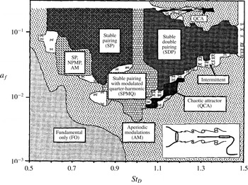
In less controlled configurations, vortex pairing events are often observed to be irregular and intermittent. Broze & Hussain (Reference Broze and Hussain1994, Reference Broze and Hussain1996) conducted jet experiments with single-frequency excitation; depending on the Strouhal number
 $St_{D}$
and on the forcing amplitude
 $a_{f}$
, different types of behaviour were reported, as summarised in figure 2. Regular dynamics was found to arise over large parameter regions, namely no pairing (FO regime in figure 2), stable pairing (SP) and stable double pairing (SDP), the latter referring to the occurrence of two successive stages of vortex pairing. Irregular dynamics was observed either in the mild form of ‘aperiodic modulations’ of the first (AM) or the second pairing stage (SPMQ), or in more erratic ways, categorised as intermittency, chaos (QCA) and ‘nearly periodic modulations’ (NPMP).
Pairing dynamics observed experimentally in turbulent jets at
 $Re=O(10^{4})$
, forced at a Strouhal number
 $St_{D}$
with amplitude
 $a_{f}$
. No subharmonic forcing is applied. From Broze & Hussain (Reference Broze and Hussain1996).

The results of Broze & Hussain (Reference Broze and Hussain1996) do not appear to depend significantly on the Reynolds number within their operating conditions of
 $11\,000\leqslant Re\leqslant 90\,000$
. Drawing on chaos theory, the authors characterised the pairing dynamics in terms of attractors. For irregular scenarios, it was demonstrated that the occurrence of pairing of two vortices is strongly influenced by previous pairing events, implying that upstream-directed feedback is involved in the subharmonic growth. This observation is fully consistent with the wave-interaction model discussed in § 2.2. Narayanan & Hussain (Reference Narayanan and Hussain1997) attempted to stabilise the pairing dynamics in chaotic regimes.
2.3.2 Pairing-related jet noise
High-speed jets are potent sources of noise, and the role of vortex pairing as an aeroacoustic source mechanism has received much attention. Bridges & Hussain (Reference Bridges and Hussain1987) determined that the radiated noise is dominated by pairing events only in cases where the initial shear layer is laminar; in fully turbulent jets, vortex pairing appears to be acoustically unimportant. The dominant role of vortex pairing in laminar jet noise was further analysed numerically by Bogey & Bailly (Reference Bogey and Bailly2010). A detailed description of sound generation from vortex interaction in jets was given by Inoue (Reference Inoue2002), and model-based predictions of radiated sound levels were derived by Schram et al. (Reference Schram, Taubitz, Anthoine and Hirschberg2005).
2.3.3 Kinematical modelling of vortex-ring interaction
Vortex interaction can be conveniently modelled by use of the Biot–Savart law. An account of early applications of such approaches to vortex rings is given by Shariff & Leonard (Reference Shariff and Leonard1992); these studies were largely concerned with the initial roll-up or with the collective motion of a limited number of co-axial vortices. A common representation characterises a vortex ring by its core centre position and core radius, from which a semi-analytical induction law can be derived (Saffman Reference Saffman1992). Contrary to vortex elements in a two-dimensional plane, axisymmetric vortex rings move at a self-induced velocity, which becomes infinitely large as the core radius approaches zero. Some simplifications arise from the assumption that the core radius is much smaller than the ring radius.
Within the limiting assumptions of inviscid flow and compact cores, such a conceptual model then yields low-dimensional systems representing the mutually induced motion of a collection of vortex rings. The ‘leap-frogging’ interaction between two rings, when one passes through the other, corresponds to the early nonlinear stage of pairing in a jet before actual merging occurs. A model of a plane jet, consisting of counter-rotating vortex pairs, was studied by Tophøj & Aref (Reference Tophøj and Aref2013), who formulated a linear stability criterion for the occurrence of leap-frogging. Similarly, Borisov, Kilin & Mamaev (Reference Borisov, Kilin and Mamaev2013) and Borisov et al. (Reference Borisov, Kilin, Mamaev and Tenenev2014) derived stability criteria for sets of two and three co-axial vortex rings, and validated these with respect to numerical simulations of viscous flow at high Reynolds number. Their work was completed by Cheng, Lou & Lim (Reference Cheng, Lou and Lim2015), who explicitly portrayed parameter regions in which leap-frogging could occur, depending on the Reynolds number and the aspect ratio of the vortex arrangement. Meunier et al. (Reference Meunier, Ehrenstein, Leweke and Rossi2002) discovered a merging criterion for two co-rotating vortices in a two-dimensional plane.
2.3.4 Pairing of helical vortices
In several industrial applications, such as helicopter rotors or wind turbines, a wake composed of several nested helical vortices is formed (Vermeer, Sørensen & Crespo Reference Vermeer, Sørensen and Crespo2003). Further downstream, these helical vortices diffuse and can interact together as well as with the hub vortex (Felli, Camussi & Di Felice Reference Felli, Camussi and Di Felice2011; Delbende, Piton & Rossi Reference Delbende, Piton and Rossi2015).
Formally, these vortices form a time-periodic three-dimensional flow, which can be regarded as a steady state in a frame of reference rotating with the blades. In addition, assuming no interaction between vortices, they diffuse slowly in the far wake, allowing for a quasi-static approximation (Selçuk, Delbende & Rossi Reference Selçuk, Delbende and Rossi2017b ) when neglecting variations of the vortex structure in the axial direction. Therefore, Selçuk, Delbende & Rossi (Reference Selçuk, Delbende and Rossi2017a ) carried out a global stability analysis of these quasi-static states reduced to steady flows. At low pitch values, they found the existence of unstable modes that trigger leap-frogging, overtaking and eventually pairing when superposed onto the quasi-static base flow.
3 Vortex pairing in simulations at various Reynolds and Strouhal numbers
In this section, we give a general overview of the vortex pairing phenomenon in axisymmetric laminar jets. After explaining the numerical simulation details, we show that, depending on the jet parameters and the forcing considered, vortex pairing can occur or not. When it does, we take a close look on a pairing sequence. Eventually, we finish with a parametric study to characterise its occurrence domain.
3.1 Set-up of direct numerical simulations
Simulations were carried out using Nek5000 (Nek 5000), an incompressible spectral element code. A perfectly axisymmetric jet is described in cylindrical coordinates
 $(z,r)$
,
 $z$
being the main flow direction and
 $r$
being the radial distance from the jet axis. The flow is assumed to be governed by the incompressible axisymmetric Navier–Stokes equations with zero azimuthal velocity, written in dimensionless form as
 $$\begin{eqnarray}\displaystyle \displaystyle \frac{\unicode[STIX]{x2202}v}{\unicode[STIX]{x2202}t}+v\frac{\unicode[STIX]{x2202}v}{\unicode[STIX]{x2202}r}+u\frac{\unicode[STIX]{x2202}v}{\unicode[STIX]{x2202}z} & = & \displaystyle -\frac{\unicode[STIX]{x2202}p}{\unicode[STIX]{x2202}r}+\frac{1}{Re}\left(\frac{1}{r}\frac{\unicode[STIX]{x2202}}{\unicode[STIX]{x2202}r}\left(r\frac{\unicode[STIX]{x2202}v}{\unicode[STIX]{x2202}r}\right)-\frac{v}{r^{2}}+\frac{\unicode[STIX]{x2202}^{2}v}{\unicode[STIX]{x2202}z^{2}}\right),\end{eqnarray}$$
 $$\begin{eqnarray}\displaystyle \displaystyle \frac{\unicode[STIX]{x2202}u}{\unicode[STIX]{x2202}t}+v\frac{\unicode[STIX]{x2202}u}{\unicode[STIX]{x2202}r}+u\frac{\unicode[STIX]{x2202}u}{\unicode[STIX]{x2202}z} & = & \displaystyle -\frac{\unicode[STIX]{x2202}p}{\unicode[STIX]{x2202}z}+\frac{1}{Re}\left(\frac{1}{r}\frac{\unicode[STIX]{x2202}}{\unicode[STIX]{x2202}r}\left(r\frac{\unicode[STIX]{x2202}u}{\unicode[STIX]{x2202}r}\right)+\frac{\unicode[STIX]{x2202}^{2}u}{\unicode[STIX]{x2202}z^{2}}\right),\end{eqnarray}$$
 $$\begin{eqnarray}\displaystyle \displaystyle \frac{1}{r}\frac{\unicode[STIX]{x2202}(rv)}{\unicode[STIX]{x2202}r}+\frac{\unicode[STIX]{x2202}u}{\unicode[STIX]{x2202}z} & = & \displaystyle 0,\end{eqnarray}$$
 $\boldsymbol{u}$
has axial and radial components
 $u$
and
 $v$
, and
 $p$
denotes pressure. The jet diameter
 $D$
and the inlet centreline velocity
 $U_{0}$
are used to render the flow problem non-dimensional, leading to a definition of the Reynolds number as
 $Re=U_{0}D/\unicode[STIX]{x1D708}$
, with
 $\unicode[STIX]{x1D708}$
the kinematic viscosity. The computational domain extends, unless specified otherwise, over
 $40\times 5$
diameters in the axial and radial directions, respectively, and it is discretised with 17 600 spectral elements, each containing 64 mesh points.
Boundary conditions are specified as follows. In the inlet plane,
 $z=0$
, a hyperbolic tangent velocity profile is imposed. Its amplitude is modulated in time as
 $$\begin{eqnarray}\boldsymbol{u}(z=0,r,t)=\frac{1}{2}\left\{1-\tanh \left[\frac{1}{4\unicode[STIX]{x1D703}_{0}}\left(r-\frac{1}{4r}\right)\right]\right\}(1+A\cos (\unicode[STIX]{x1D714}_{f}t))\boldsymbol{e}_{z},\end{eqnarray}$$
where
 $A$
is the forcing amplitude,
 $\unicode[STIX]{x1D703}_{0}=0.025$
is the initial non-dimensional shear layer thickness and
 $\unicode[STIX]{x1D714}_{f}$
is the forcing frequency. The forcing period is given by
 $T=2\unicode[STIX]{x03C0}/\unicode[STIX]{x1D714}_{f}$
, and the Strouhal number is defined as
 $St_{D}=\unicode[STIX]{x1D714}_{f}D/(2\unicode[STIX]{x03C0}U_{0})$
.
On the jet centreline, axisymmetric boundary conditions are imposed as
 $$\begin{eqnarray}\frac{\unicode[STIX]{x2202}u}{\unicode[STIX]{x2202}r}=v=\frac{\unicode[STIX]{x2202}p}{\unicode[STIX]{x2202}r}=0\quad \text{at }r=0.\end{eqnarray}$$
In the outlet plane,
 $z_{max}=40$
, and on the lateral boundary,
 $r_{max}=5$
, the standard outflow formulation provided by Nek5000 is employed. This prescribes a stress-free condition
 $$\begin{eqnarray}\frac{1}{Re}\frac{\unicode[STIX]{x2202}v}{\unicode[STIX]{x2202}r}-p=\frac{\unicode[STIX]{x2202}u}{\unicode[STIX]{x2202}r}=0\quad \text{at }r=r_{max}\quad \text{and}\quad \frac{1}{Re}\frac{\unicode[STIX]{x2202}u}{\unicode[STIX]{x2202}z}-p=\frac{\unicode[STIX]{x2202}v}{\unicode[STIX]{x2202}z}=0\quad \text{at }z=z_{max}.\end{eqnarray}$$
The flow configuration is thus characterised by the Reynolds number
 $Re$
, the Strouhal number
 $St_{D}$
, the initial shear layer thickness
 $\unicode[STIX]{x1D703}_{0}$
and the forcing amplitude
 $A$
. A single value
 $\unicode[STIX]{x1D703}_{0}=0.025$
is used throughout this study.
3.2 Two distinct behaviours
Depending on flow parameters and forcing Strouhal number, rolled-up vortices may spontaneously undergo subsequent pairing. In the absence of free-stream turbulence, and if the harmonic forcing is well controlled, this pairing takes place in a perfectly regular fashion.
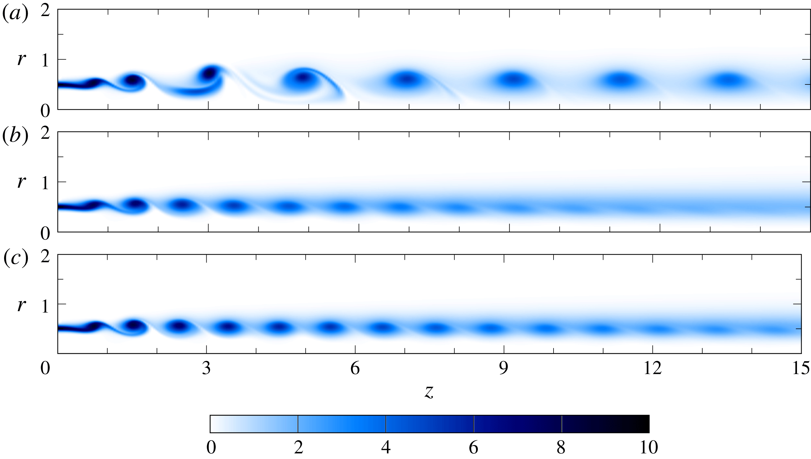
In cases where pairing occurs, two neighbouring vortices merge into one, such that the passage frequency of vortices downstream of the pairing location is exactly half that of the imposed forcing. An example, obtained by direct numerical simulation with parameters
 $Re=2000$
,
 $St_{D}=0.6$
and
 $A=5\,\%$
, is shown in figure 3(a). If the forcing is characterised by the time period
 $T$
, the ‘paired state’ is globally 2
 $T$
-periodic. The velocity field of a paired state will be denoted
 $\boldsymbol{u}^{p}$
.
Vorticity snapshots of the periodic paired and unpaired states, obtained naturally for two different parameter settings. Forcing amplitude, Reynolds and Strouhal numbers are defined in § 3.1. (a) Paired state (
 $2T$
-periodic) at
 $St_{D}=0.6$
,
 $Re=2000$
and
 $A=5\,\%$
at
 $t=3T/2$
. This is the same state as in figure 4(d). (b) Unpaired state (
 $T$
-periodic) at
 $St_{D}=0.6$
,
 $Re=1300$
and
 $A=5\,\%$
at
 $t=T/2$
. (c) Unpaired state (
 $T$
-periodic) stabilised using time-delayed feedback control, defined in § 4.1, at
 $St_{D}=0.6$
,
 $Re=2000$
and
 $A=5\,\%$
at
 $t=T/2$
.

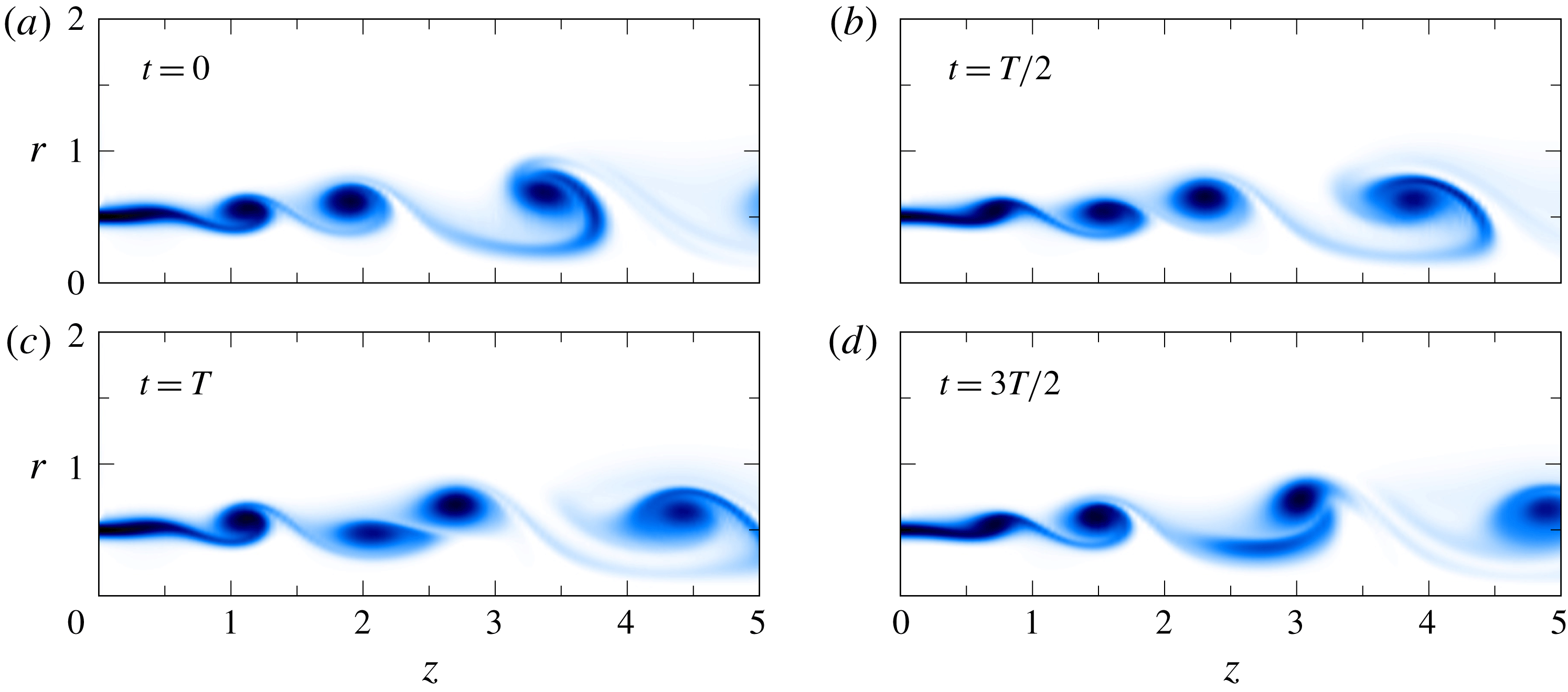
Vorticity snapshots of a paired case at
 $Re=2000$
forced harmonically at
 $St_{D}=0.60$
and
 $A=5\,\%$
. Only the region near the inlet is shown. The colour coding is the same as in figure 3.

A different behaviour is observed when the Reynolds number is lowered to
 $Re=1300$
, as shown in figure 3(b). Vortices roll up close to the nozzle and advect downstream, until they are dissipated by viscosity, but no spontaneous pairing is observed at this parameter setting. Such a flow state is globally
 $T$
-periodic and will be called hereafter an ‘unpaired state’. Its velocity field will be denoted
 $\boldsymbol{u}^{u}$
.
When the natural time-asymptotic flow state for a given set of parameters involves pairing, it is still possible to recover an unpaired state as an alternative solution of the flow equations, by use of time-delayed feedback control (see § 4.1 and Shaabani-Ardali et al.
Reference Shaabani-Ardali, Sipp and Lesshafft2017). The unpaired state obtained in such a way for the previous configuration with
 $Re=2000$
is shown in figure 3(c). This solution is an exact solution of the Navier–Stokes equations without the time-delayed feedback.
3.3 The dynamics of vortex pairing
The process of the pairing of two vortices is inspected from snapshots of the vorticity, presented in figure 4, at four different phases of one pairing cycle. At
 $t=0$
(figure 4
a), two successive vortices, located around
 $z=1$
and
 $2$
, have rolled up due to the primary shear instability. One half-cycle of the forcing period later (figure 4
b), the leading vortex has slightly expanded radially, while the trailing one has contracted. This movement is accompanied by a deceleration of the expanding vortex, and inversely an acceleration of the contracting vortex, through the influence of the vortex-ring radius on its self-induced propulsion. The same process continues at
 $t=T$
(figure 4
c), when the trailing vortex begins to pass through the interior of the leading vortex. At
 $t=3T/2$
(figure 4
d), both vortices are in the process of merging into one, which is largely achieved at the end of the cycle (figure 4
a).
Conceptual arguments for the occurrence of vortex pairing in the literature are typically based on the interaction between fundamental and subharmonic fluctuations, and the possibility of energy transfer to the latter (Monkewitz Reference Monkewitz1988). Spatial energy variations of the fundamental
 $\unicode[STIX]{x1D714}_{f}$
and the subharmonic
 $\unicode[STIX]{x1D714}_{f}/2$
Fourier modes are readily extracted from the present numerical simulations. These are presented in figure 5, for the configuration
 $Re=2000$
,
 $St_{D}=0.6$
and
 $A=5\,\%$
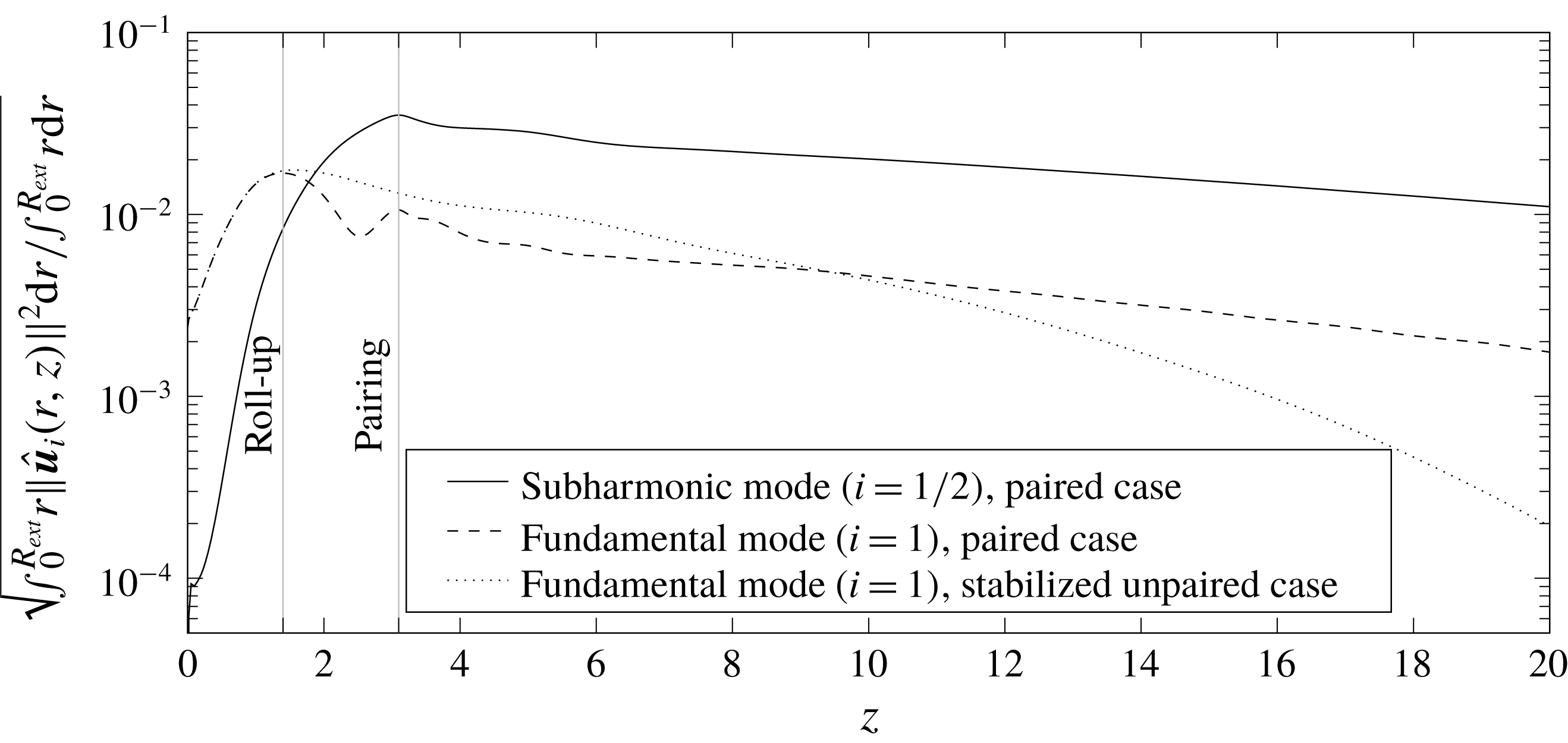
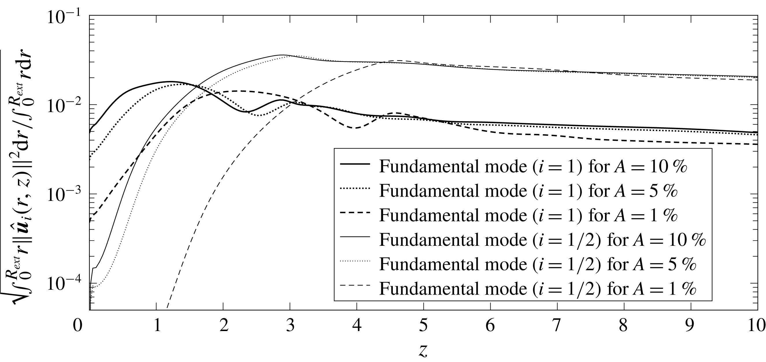
, in the form of radially integrated kinetic energy. This plot allows the distinction of various stages in the pairing process. Immediately downstream of the inlet, the fundamental mode grows from its forced initial amplitude to its peak value at
 $z=1.4$
. This streamwise position may be identified with the shedding of a fully formed vortex (see figure 4). The subharmonic component experiences strong exponential growth over the same interval, starting from a much lower level, as the boundary condition imposes zero amplitude at the inlet. Subharmonic growth continues down to
 $z=3.1$
, where figure 4(d) shows strong pairing dynamics. The energy of the fundamental mode decreases over the distance
 $1.4<z<3.1$
, although a local maximum is found at the peak location of the subharmonic mode. As pairing is accomplished, at
 $z>3.1$
, both the fundamental and the subharmonic mode decay slowly in
 $z$
, both at a similar rate, due to viscous dissipation of the convecting vortices.
Total energy of the fundamental
 $\hat{\boldsymbol{u}}_{1}$
and subharmonic
 $\hat{\boldsymbol{u}}_{1/2}$
Fourier components in each plane
 $z=\text{const.}$
as a function of
 $z$
at
 $St_{D}=0.6$
,
 $Re=2000$
and
 $A=5\,\%$
.

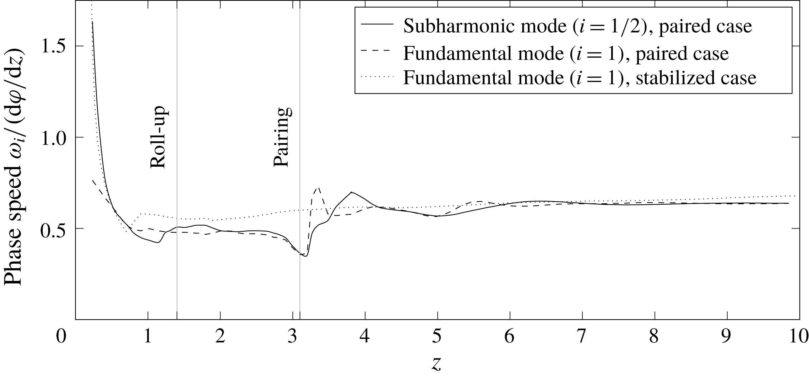
Consistent with these observations, Monkewitz (Reference Monkewitz1988) argued that a growth of subharmonic perturbations must be fed by energy transfer from the fundamental mode, which requires that both modes propagate at the same phase velocity. Phase velocities of fundamental and subharmonic fluctuations in the present simulation are compared in figure 6 as solid and dashed lines. The reported phase velocities are measured, for each streamwise location, at the radial distance where each respective Fourier mode has its maximum amplitude along
 $r$
. The values for both modes match quite closely throughout the relevant interval upstream of the pairing location. They continue to match in the downstream region, but this is only the result of the fundamental mode being slaved to its subharmonic counterpart as a passive harmonic.
Phase speed along the line of maximum subharmonic mode of the subharmonic and fundamental modes of a paired jet at
 $(Re=2000,St_{D}=0.60)$
, and comparison with the phase speed of the fundamental mode along the lime of maximum fundamental mode of the corresponding stabilised (unpaired) jet. The phase of the Fourier mode is denoted as
 $\unicode[STIX]{x1D711}$
.

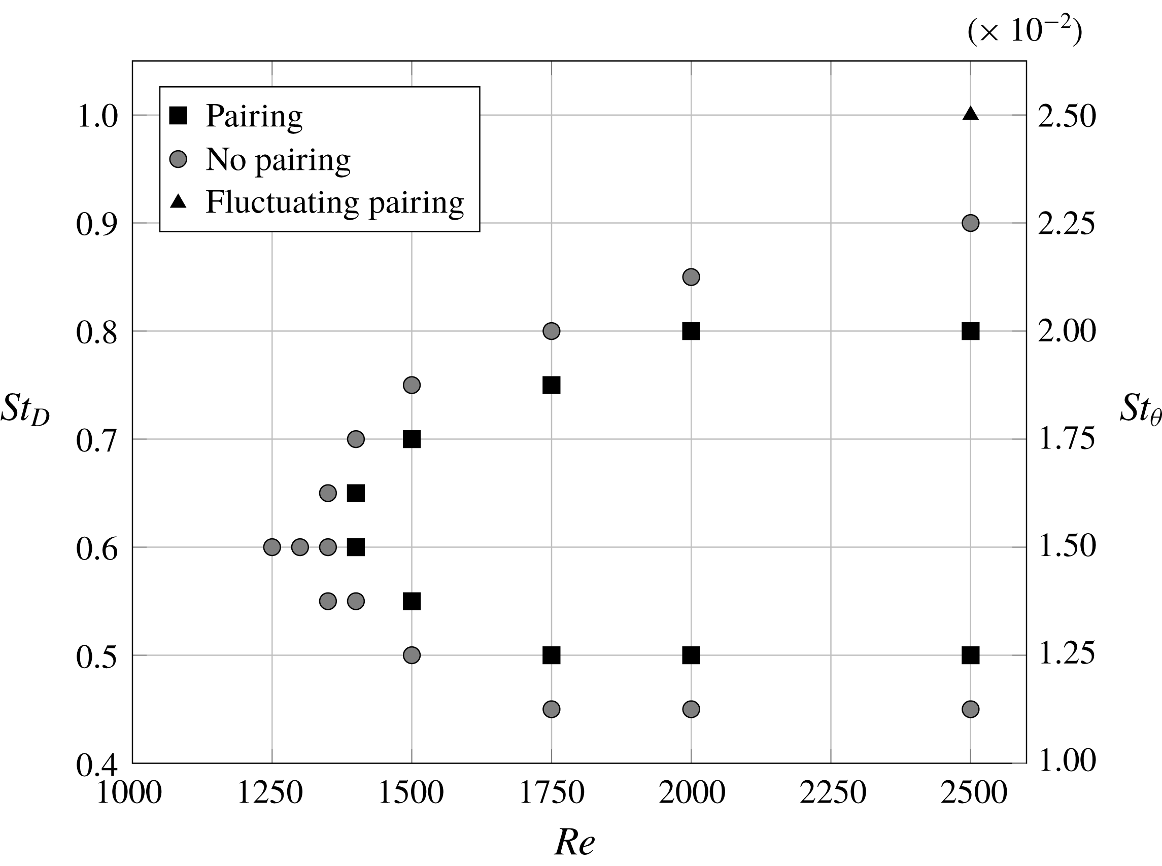
Occurrence of vortex pairing as a function of Reynolds number and Strouhal number for configurations with forcing amplitude
 $A=5\,\%$
and initial shear layer thickness
 $\unicode[STIX]{x1D703}_{0}=0.025$
. Only points near the pairing boundary are represented.

For comparison, energy and phase velocity results obtained for the fundamental mode of the corresponding stabilised (unpaired) flow are also presented in figures 5 and 6 (dotted lines), alongside the values found in the paired state. Upstream of the roll-up location, the fundamental modes show identical energy growth in both configurations. Between the roll-up and the pairing locations, the fundamental energy decay in the paired case is stronger than in the unpaired case, which again indicates that the growth of subharmonic perturbations feed on the energy of the fundamental mode. However, downstream of the pairing location, the fundamental mode in the stabilised case decays significantly faster, and at an increasing rate. This difference is also visible when one compares figures 3(a) and 3(c): it appears that the lower frequency and the stronger circulation of the paired vortices hinder their diffusion and allow them to be sustained longer. When comparing the phase velocities in figure 6, it is seen that the unpaired fundamental mode propagates faster than its paired counterpart upstream of the pairing location, whereas their velocities are again equal in the downstream region. The discrepancy upstream of the pairing can be linked to different positions of the vortices: in the paired case, the vortices are radially more expanded than in the unpaired case, therefore moving at a slower speed. Vortex pairing not only influences the flow downstream, but also upstream.
3.4 Parametric study
All simulations presented in this section were carried out on a domain with
 $z_{max}=15$
in order to save computational resources. Test runs with
 $z_{max}=40$
were performed for selected cases, showing no effect of domain truncation on the results presented here.
3.4.1 Effect of Reynolds number and Strouhal number
The effect of Reynolds and Strouhal numbers on the onset of vortex pairing is investigated first, for a fixed forcing amplitude
 $A=5\,\%$
. Direct numerical simulations were run, first in an exploratory fashion for many (
 $Re,St_{D}$
) combinations. After an initial transient phase, the flow settles into an asymptotic time-periodic state. Asymptotic states that involve regular vortex pairing were found in a restricted region in the (
 $Re,St_{D}$
) plane, and the boundary of that region was then determined more accurately by running simulations well into the asymptotic regime. Results of these simulations are mapped in figure 7. Pairing is found to occur first around a critical Reynolds number
 $Re_{c}=1375$
, for the fundamental forcing Strouhal number
 $St_{D}=0.6$
. Up to
 $Re=2500$
, the maximum value considered in this study, vortex pairing at asymptotic times is restricted to the band
 $0.5\leqslant St_{D}\leqslant 0.8$
. With increasing Reynolds number, the pairing becomes more vigorous, and its location gradually shifts nearer to the inlet.
Close to the instability thresholds, it becomes difficult to precisely characterise the flow behaviour, because of the long simulation times needed to achieve convergence. When the Reynolds number is approximately 1350, computations were run on full-length domains (
 $40D$
), and even after several hundred forcing periods, the paired or unpaired nature of the final flow state cannot be determined. For instance, at
 $St_{D}=0.6$
, the final state for
 $Re=1350$
is unpaired, for
 $Re=1400$
it is paired. For intermediate values
 $Re=1360$
, 1372 or 1375 (close to threshold
 $Re_{c}=1371$
predicted in § 4.4), the pairing location moves gradually downstream as time evolves, but with no indication whether it will eventually become stationary. These ambiguous data points are not displayed in figure 7.
As mentioned in § 2.1, a first parametric study of vortex pairing in terms of Reynolds and Strouhal numbers has been carried out experimentally by Zaman & Hussain (Reference Zaman and Hussain1980), for Reynolds numbers greater than
 $10^{4}$
and thin initial mixing layer (
 $\unicode[STIX]{x1D703}/D\approx 0.25\,\%$
). They found that pairing could occur in two frequency bands, one characterised by a Strouhal number
 $St_{\unicode[STIX]{x1D703}}=f\unicode[STIX]{x1D703}/U$
based on the shear layer thickness, the other by a Strouhal number
 $St_{D}=fD/U$
based on the jet diameter. Pairing has been reported for
 $St_{\unicode[STIX]{x1D703}}$
around 0.012 and for
 $0.75\leqslant St_{D}\leqslant 1.0$
. With our choice of the initial shear layer thickness being 5 % of the diameter, these two regimes are only weakly separated, which explains why our findings of a single band of instability at a given Reynolds is coherent; both scalings are indicated in figure 7.
Again for Reynolds numbers greater than
 $10^{4}$
, and for a 5 % forcing amplitude, Broze & Hussain (Reference Broze and Hussain1994) found several flow regimes depending on
 $St_{D}$
(see figure 2): no pairing for
 $St_{D}<0.52$
, aperiodic modulations and coexistence of different states (stable or modulated pairing) for
 $0.52<St_{D}<0.77$
, stable pairing for
 $0.77<St_{D}<0.97$
, stable pairing with quarter-harmonic modulations for
 $0.97<St_{D}<1.02$
and stable double pairing for
 $St_{D}>1.02$
, with some intermittent cases. The
 $St_{\unicode[STIX]{x1D703}}$
dependence is not documented in that study. In our computations, we do not encounter such a richness of scenarios, because our inlet condition is fully laminar and time periodic, and because our Reynolds number is one decade lower; however, the occurrence of pairing, reported in figure 7, is consistent with the experiments of Broze & Hussain (Reference Broze and Hussain1994). Multiple stages of successive pairing are never observed in our computations, even at
 $St_{D}>1$
. This difference with respect to the experiments is certainly owing to the lower Reynolds number, as Cheng et al. (Reference Cheng, Lou and Lim2015) demonstrated that viscosity inhibits pairing. However, the modulated states described by Broze & Hussain (Reference Broze and Hussain1994) for
 $St_{D}\approx 1$
may be linked to our observation of fluctuations of the pairing position (triangle in figure 7).
Cheng et al. (Reference Cheng, Lou and Lim2015) investigated numerically the leap-frogging of coaxial vortex rings. For a system of two adjacent vortices, they systematically documented the occurrence of leap-frogging as a function of Reynolds number and vortex separation. The Reynolds number, defined as the ratio of the ring vorticity over the viscosity and chosen to be of the order of
 $10^{3}$
, is related to the product between Reynolds and Strouhal numbers in our present notation. The ratio of the vortex spacing over the ring radius is related to the inverse of the Strouhal number as defined here. Cheng et al. (Reference Cheng, Lou and Lim2015) found that leap-frogging occurs only above a critical Reynolds number, and for a narrow Strouhal band that increases with Reynolds number. This is consistent with our findings (figure 7), as pairing can be understood as an advanced stage of leap-frogging (figure 4).
3.4.2 Effect of forcing amplitude
The effect of forcing amplitude is investigated by including computations with two additional values,
 $A=1\,\%$
and 10 %. Instability maps in the
 $(Re,St_{D})$
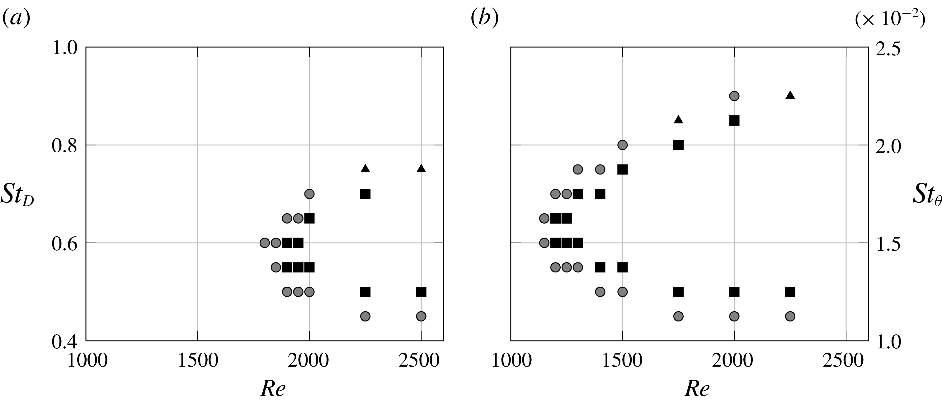
plane for these configurations are displayed in figure 8(a,b). An increase in the forcing amplitude is seen to shift the onset of pairing towards lower Reynolds number values.
Occurrence of vortex pairing as a function of the Reynolds and the Strouhal number for two different forcing amplitudes
 $A=1\,\%$
and 10 %. The same symbols as in figure 7 are used.

Total energy of the fundamental and subharmonic modes in each plane
 $z=\text{const.}$
as a function of
 $z$
at
 $St_{D}=0.6$
and
 $Re=2000$
. Three values of the inlet forcing amplitude are considered,
 $A=1\,\%$
, 5 % and 10 %.

Another effect of increasing
 $A$
is to move the roll-up and pairing locations upstream, as can be seen in figure 9. In the same way as discussed for figure 5, the energy of the fundamental mode in all cases grows from the inflow towards its maximum at the roll-up location, whereas the subharmonic mode peaks at the location of pairing. Increasing the fundamental amplitude at the inflow reduces the distance needed before roll-up, and it catalyses the subharmonic mode, inducing an earlier pairing.
However, by comparing the difference between the modes at
 $A=1\,\%$
and 5 %, and between the modes at
 $A=5\,\%$
and 10 % in figure 9, it is anticipated that a further increase in
 $A$
will only marginally change the paired flow behaviour. This is consistent with Broze & Hussain (Reference Broze and Hussain1994): as shown in figure 2, increasing the forcing amplitude above 5 % does not induce significant topological changes in the final state, but below 1 % forcing, no stable pairing is observed in the experiments. Raman & Rice (Reference Raman and Rice1991) also found that a critical minimal amplitude of the fundamental forcing was required to trigger pairing. Therefore, an expansion of the study to lower amplitude levels
 $A<1\,\%$
could be of interest; however, this would require higher values of
 $Re$
to be considered, rendering the assumption of laminar flow increasingly doubtful.
In their leap-frogging study of two vortex rings, Cheng et al. (Reference Cheng, Lou and Lim2015) varied the vortex thickness, and thereby the vortex concentration, which is similar to varying the amplitude of forcing. Consistent with the present study, they concluded that stronger vortices undergo pairing at lower Reynolds numbers.
3.4.3 Effect of inlet noise
In configurations where vortex pairing does not arise intrinsically, the flow may still be receptive to low-level subharmonic extrinsic perturbations, in the sense of a ‘slightly damped oscillator’ (Huerre & Monkewitz Reference Huerre and Monkewitz1990), and exhibit vortex pairing in their presence. In the following, this receptivity is probed by imposing a random noise in addition to the fundamental forcing at the inlet, such that the inflow condition is prescribed as
 $$\begin{eqnarray}\boldsymbol{u}(r,t)=\frac{1}{2}\left\{1-\tanh \left[\frac{1}{4\unicode[STIX]{x1D703}_{0}}\left(r-\frac{1}{4r}\right)\right]\right\}(1+A\cos (\unicode[STIX]{x1D714}_{f}t)+\unicode[STIX]{x1D716}_{noise}(t))\boldsymbol{e}_{\boldsymbol{z}},\end{eqnarray}$$
with
 $\unicode[STIX]{x1D716}_{noise}$
a white noise, constant in
 $r$
, with a specified standard deviation. Four Reynolds number values are selected,
 $Re=500$
, 750, 1000 and 1300, and two values of the standard deviation
 $A_{\unicode[STIX]{x1D716}}=\sqrt{\langle \unicode[STIX]{x1D716}_{noise},\unicode[STIX]{x1D716}_{noise}\rangle }=0.1\,\%$
and 1 % are tested. The latter are chosen such as not to exceed the level of coherent forcing
 $A$
. The fundamental forcing in all cases is prescribed with
 $St_{D}=0.6$
and
 $A=5\,\%$
.
Four distinct types of the flow response are observed:
(i) At low Reynolds number, the noise barely impacts the flow behaviour. For instance, at
 $Re=500$
and for both noise levels, no significant departure from the purely harmonically forced jet is observed.
(ii) The noise induces a subharmonic modulation of the vortices, but the flow diffuses too quickly for pairing to occur, for instance in the case
$Re=750$
and
$A_{\unicode[STIX]{x1D716}}=0.1\,\%$
.(iii) Intermittent pairing is triggered, for instance at
$Re=1000$
and
$A_{\unicode[STIX]{x1D716}}=0.1\,\%$
, or at
$Re=750$
and
$A_{\unicode[STIX]{x1D716}}=1.0\,\%$
(figure 10). In the latter case, pairing occurs far downstream, where the vortices are indistinct due to diffusion.(iv) Continuous pairing is sustained by noise input, but its location fluctuates in time. This is observed for
$Re=1000$
with
$A_{\unicode[STIX]{x1D716}}=1\,\%$
, and for
$Re=1300$
with
$A_{\unicode[STIX]{x1D716}}=0.1\,\%$
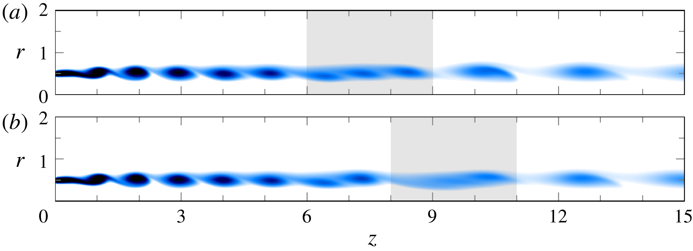
(figure 11) as well as 1.0 %. As described experimentally by Ho & Huang (Reference Ho and Huang1982), Husain & Hussain (Reference Husain and Hussain1989), other phenomena such as shredding, where one single vortex ‘escapes’ between two successful pairing events, or collective interaction, where more than two vortices interact at once, can be observed, for instance in figure 12.


Vorticity snapshots at
 $Re=750$
,
 $St_{D}=0.60$
and
 $A=5\,\%$
with
 $A_{\unicode[STIX]{x1D716}}=1.0\,\%$
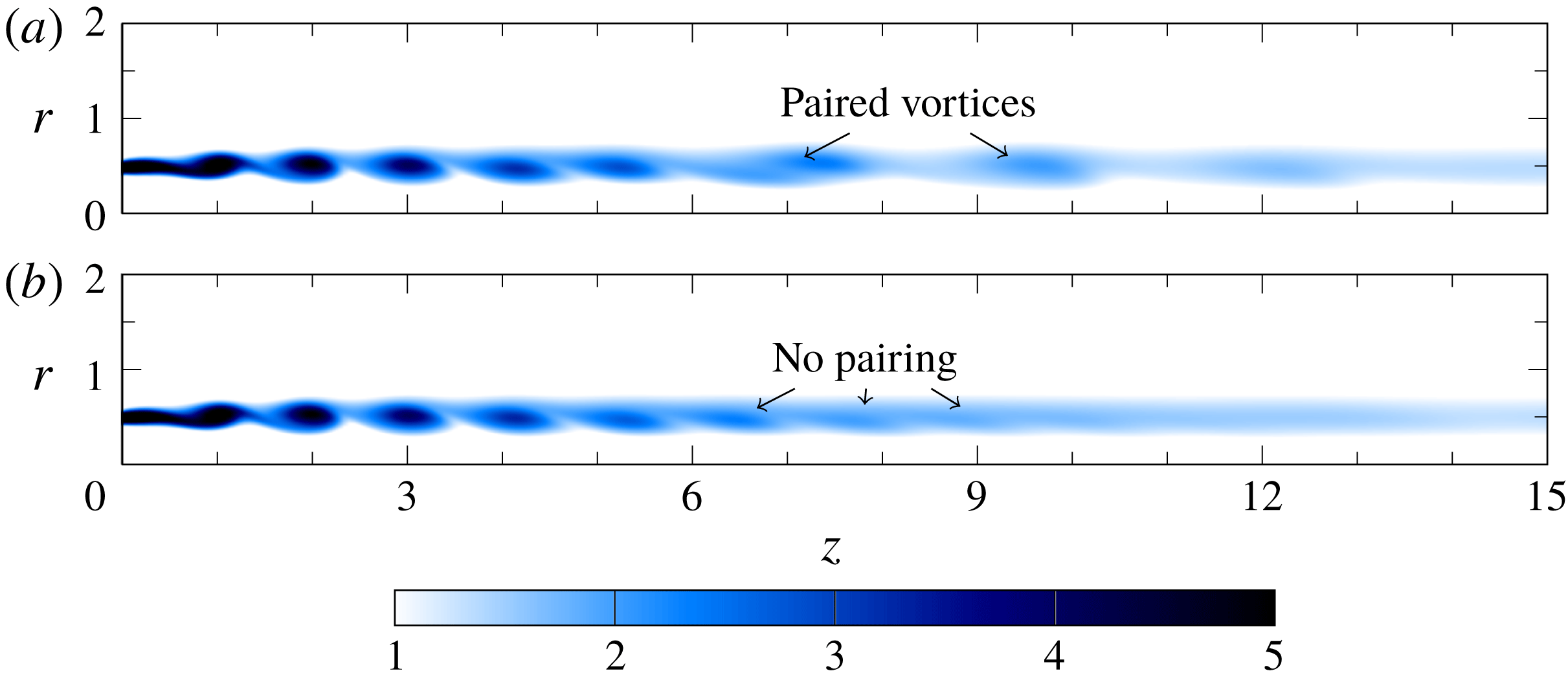
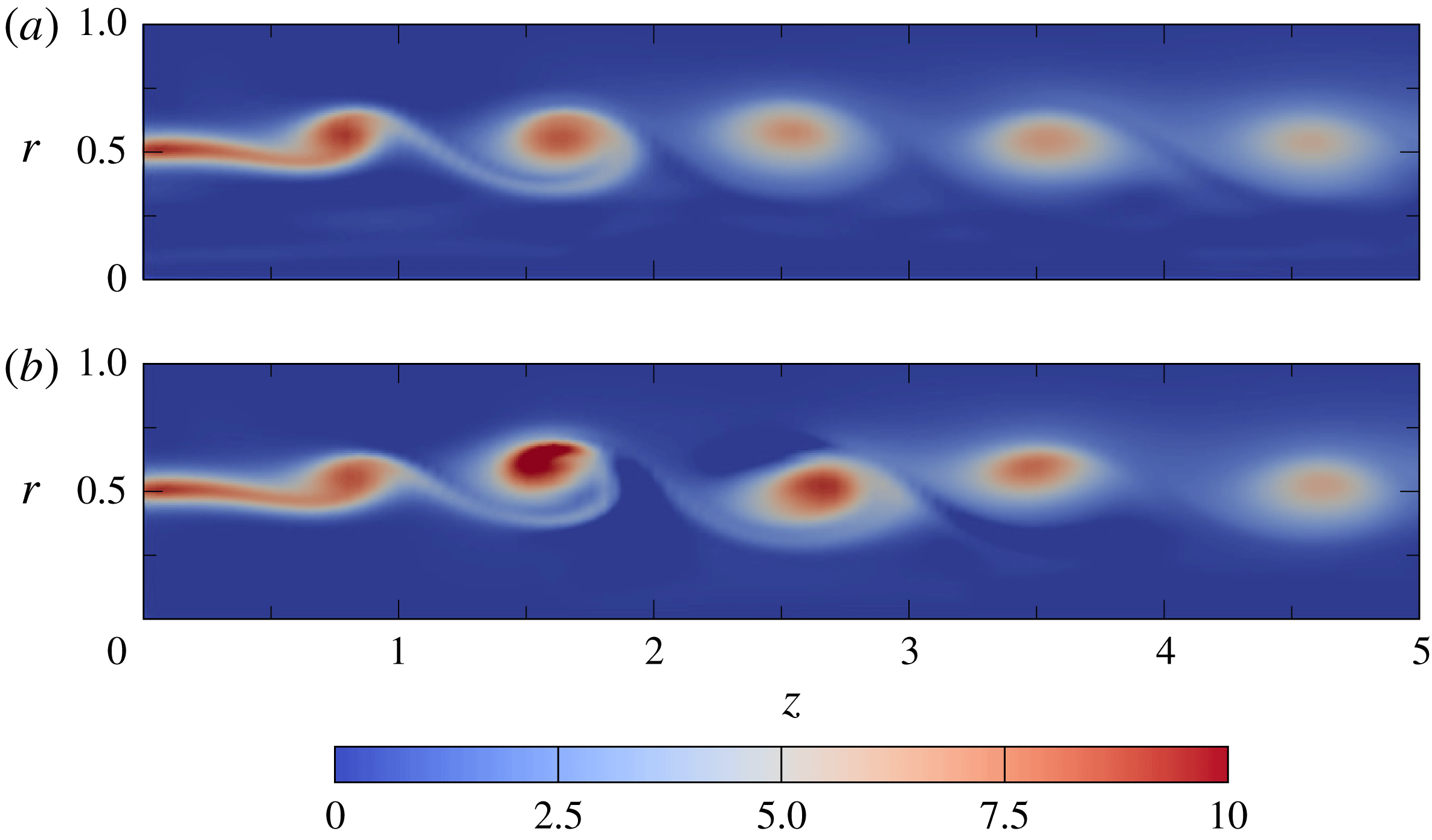
taken at two different times, and both at the same phase. Pairing is intermittent, occurring in (a) and not in (b). The colour bar is rescaled compared to figure 3(b), to magnify the behaviour of downstream vortices.

Vorticity snapshots at
 $Re=1300$
and
 $St_{D}=0.60$
with
 $A_{\unicode[STIX]{x1D716}}=0.1\,\%$
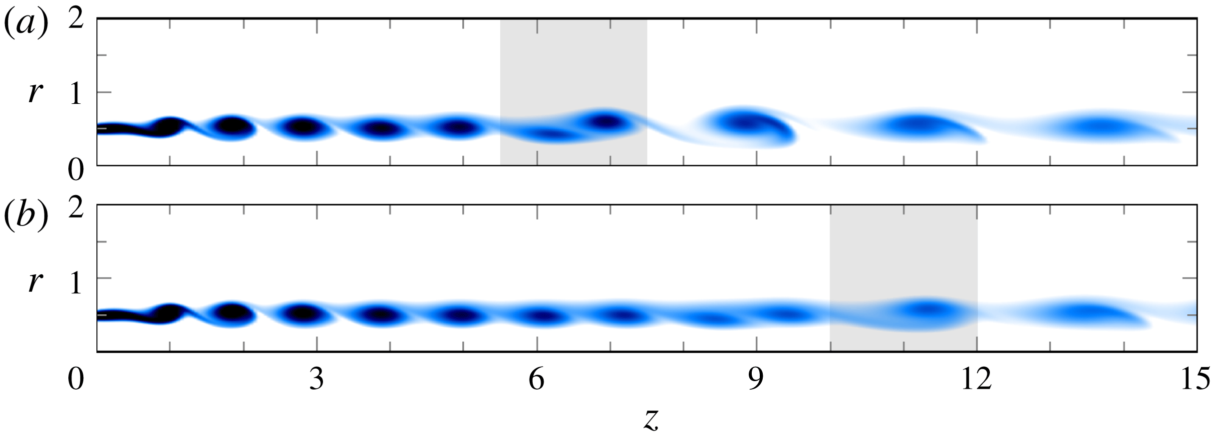
taken at two different times, and both at the same phase. This shows the pairing location fluctuation, emphasised in grey, in this set-up. The colour bar is in figure 10.

Vorticity snapshots at
 $Re=1000$
and
 $St_{D}=0.60$
with
 $A_{\unicode[STIX]{x1D716}}=1.0\,\%$
: (b) is taken two forcing periods after (a). The three vortices located in the shaded area in (a) merge altogether in (b), as an example of collective interaction. The colour bar is in figure 10.

4 Vortex pairing as an unstable global Floquet mode
In this section, we investigate whether the onset of vortex pairing can be described as the manifestation of a global Floquet instability of the periodic unpaired state. This unpaired state must first be computed for a given combination of flow parameters (§ 4.1). After a short reminder of Floquet theory (§ 4.2), and a presentation of the numerical implementation (§ 4.3), the linear Floquet stability of the unpaired vortex street is analysed (§ 4.4), and the instability characteristics are compared to the observations documented in the previous section.
4.1 Computation of
$T$
-periodic states without vortex pairing

Periodic flow states are obtained through direct numerical simulation, as described in § 3.1. In order to suppress vortex pairing in configurations where it naturally arises, subharmonic fluctuations are actively damped by means of time-delayed feedback control. A short description of this method follows, for details the reader is referred to Shaabani-Ardali et al. (Reference Shaabani-Ardali, Sipp and Lesshafft2017).
A fully synchronised paired state can be decomposed into one component that is
 $T$
-periodic and another that is only
 $2T$
-periodic,
 $$\begin{eqnarray}\displaystyle \boldsymbol{u}^{p}(\boldsymbol{x},t) & = & \displaystyle \mathop{\sum }_{n}\boldsymbol{u}_{n}^{T}(\boldsymbol{x})\exp (\text{i}n\unicode[STIX]{x1D714}_{f}t)+\mathop{\sum }_{n}\boldsymbol{u}_{n}^{2T}(\boldsymbol{x})\exp \left(\text{i}\frac{2n+1}{2}\unicode[STIX]{x1D714}_{f}t\right),\nonumber\\ \displaystyle & & \displaystyle \quad \text{with }n=0,\pm 1,\pm 2,\ldots ,\pm N.\end{eqnarray}$$
In a
 $T$
-periodic unpaired state, the second sum is zero. Time-delayed feedback control is applied by adding a forcing term of the form
 $$\begin{eqnarray}\boldsymbol{f}=-\unicode[STIX]{x1D706}(\boldsymbol{u}(t)-\boldsymbol{u}(t-T)),\end{eqnarray}$$
to the right-hand side of the governing equations (3.1a
)–(3.1c
). Such forcing attenuates all
 $2T$
-periodic fluctuations, but leaves
 $T$
-periodic components unaffected. The simulations converge towards a purely
 $T$
-periodic state, in which the artificial forcing term vanishes. This solution is therefore a full solution of the Navier–Stokes equations. An example of such a stabilised unpaired state is shown in figure 3(c).
The value of
 $\unicode[STIX]{x1D706}$
in (4.2) affects the convergence of the stabilisation procedure. In a previous publication (Shaabani-Ardali et al.
Reference Shaabani-Ardali, Sipp and Lesshafft2017), it has been demonstrated that very small values of
 $\unicode[STIX]{x1D706}$
do not lead to convergence, as the resulting damping is insufficient to counteract the natural instability of the system. Similarly, too large values of
 $\unicode[STIX]{x1D706}$
result in overshooting of the damping force, which also inhibits convergence. An optimal value
 $\unicode[STIX]{x1D706}=0.0432\unicode[STIX]{x1D714}_{f}$
was derived from a model problem, and has been used in the present calculations.
4.2 Floquet framework
The Floquet stability problem for a
 $T$
-periodic unpaired base flow
 $(\boldsymbol{U}^{\boldsymbol{u}}(t),P^{u}(t))$
is set up by superposing small-amplitude perturbations
 $(\boldsymbol{u}^{\prime },p^{\prime })$
, which are governed to leading order by the linear equations
 $$\begin{eqnarray}\frac{\unicode[STIX]{x2202}\boldsymbol{u}^{\prime }}{\unicode[STIX]{x2202}t}+(\boldsymbol{U}^{\boldsymbol{u}}(t)\boldsymbol{\cdot }\unicode[STIX]{x1D735})\boldsymbol{u}^{\prime }+(\boldsymbol{u}^{\prime }\boldsymbol{\cdot }\unicode[STIX]{x1D735})\boldsymbol{U}^{\boldsymbol{u}}(t)=-\unicode[STIX]{x1D735}p^{\prime }+\frac{1}{Re}\unicode[STIX]{x0394}\boldsymbol{u}^{\prime },\quad \unicode[STIX]{x1D735}\boldsymbol{\cdot }\boldsymbol{u}^{\prime }=0.\end{eqnarray}$$
The following boundary conditions are implemented. In the inlet plane, the flow is unperturbed,
 $\boldsymbol{u}^{\prime }(r,z=0,t)=\mathbf{0}$
. We do not allow perturbations directly at the inlet, since we consider only the behaviour of intrinsic perturbations. On the centreline of the jet,
 $r=0$
, axisymmetric boundary conditions as in the nonlinear case are imposed,
 $\unicode[STIX]{x2202}_{r}u^{\prime }=v^{\prime }=\unicode[STIX]{x2202}_{r}p^{\prime }=0$
. In the outlet plane
 $z=40$
and on the lateral boundary
 $r=5$
, stress-free conditions (3.4) are chosen.
The equations are written in compact form as
 $$\begin{eqnarray}\frac{\unicode[STIX]{x2202}\boldsymbol{q}^{\prime }}{\unicode[STIX]{x2202}t}={\mathcal{L}}(t)\boldsymbol{q}^{\prime },\end{eqnarray}$$
where
 $\boldsymbol{q}^{\prime }=(\boldsymbol{u}^{\prime },p^{\prime })$
represents the perturbation state vector.
According to Floquet theory (Floquet Reference Floquet1883), one may seek modal solutions of (4.4) in the form
 $$\begin{eqnarray}\boldsymbol{q}^{\prime }(t)=P(t)\text{e}^{\unicode[STIX]{x1D63C}t}\boldsymbol{q}^{\prime }(0),\end{eqnarray}$$
with
 $P(t)$
a
 $T$
-periodic and
 $\unicode[STIX]{x1D63C}$
a constant matrix. Noting that
 $$\begin{eqnarray}\boldsymbol{q}^{\prime }(T)=\text{e}^{\unicode[STIX]{x1D63C}T}\boldsymbol{q}^{\prime }(0),\end{eqnarray}$$
due to
 $P(T)=P(0)=Id$
, the time-shift operator
 $\unicode[STIX]{x1D6F7}=\text{e}^{\unicode[STIX]{x1D63C}T}$
is introduced, such that
 $\boldsymbol{q}^{\prime }(nT)=\unicode[STIX]{x1D6F7}^{n}\boldsymbol{q}^{\prime }(0)$
. The eigenvalues
 $\unicode[STIX]{x1D707}_{i}$
of
 $\unicode[STIX]{x1D6F7}$
are known as Floquet multipliers, and the associated eigenmodes
 $v_{i}$
are the Floquet modes of the system (4.4). For a modal perturbation
 $\boldsymbol{q}^{\prime }(0)=(\tilde{\boldsymbol{v}_{i}},\tilde{p}_{i})$
, the Floquet multiplier
 $\unicode[STIX]{x1D707}_{i}$
such that
 $\boldsymbol{q}^{\prime }((n+1)T)=\unicode[STIX]{x1D707}_{i}\boldsymbol{q}^{\prime }(nT)$
represents the complex amplitude gain over one cycle period. Therefore, the stability of the system is indicated by the modulus of
 $\unicode[STIX]{x1D707}_{i}$
: if all Floquet multipliers have a modulus lower than unity, all perturbations decay at long time and the system is stable. Floquet modes with an associated
 $|\unicode[STIX]{x1D707}_{i}|>1$
experience exponential temporal growth.
The complex phase of a Floquet multiplier,
 $\arg (\unicode[STIX]{x1D707}_{i})$
, characterises the time periodicity of its associated mode. At zero phase, the mode evolves with the same periodicity as the base flow, and may be qualified as being harmonic. A phase of
 $\arg (\unicode[STIX]{x1D707}_{i})=\unicode[STIX]{x03C0}$
, indicates that two base flow periods are needed to complete one perturbation cycle, and the mode therefore evolves as
 $\unicode[STIX]{x1D714}_{f}/2$
. Such a mode is qualified as being subharmonic. As vortex pairing is a
 $2T$
-periodic phenomenon, subharmonic Floquet modes are expected to arise. Floquet multiplier phases that are not integer multiples of
 $\unicode[STIX]{x03C0}$
characterise modes with periodicities unrelated to that of the base flow.
A standard result of Floquet theory applied to the linearised Navier–Stokes equations is that the time derivative of the base flow,
 $(\unicode[STIX]{x2202}_{t}\boldsymbol{U}^{\boldsymbol{u}},\unicode[STIX]{x2202}_{t}P^{u})$
, represents a neutral Floquet mode of the system, with
 $\unicode[STIX]{x1D707}=1$
. However, such a mode does not exist in the present problem, because it is inconsistent with the boundary conditions. While the base flow is periodically forced at the inlet boundary, according to (3.2), linear perturbations are prescribed to be zero there.
4.3 Numerical implementation
The evolution of the linearised system (4.4) is calculated using a fully implicit finite-difference time-stepping scheme of second order implemented in FreeFem
 $++$
(Hecht Reference Hecht2012). The mesh has the same size and resolution as the one used in the Nek5000 calculations.
 $P2$
finite elements are used for the velocity perturbation whereas
 $P1$
finite elements are used for the pressure.
In the numerical implementation of the Floquet mode calculation, only the velocity perturbation
 $\boldsymbol{u}^{\prime }$
is considered. This is possible in incompressible flow, since the full state
 $\boldsymbol{q}^{\prime }=(\boldsymbol{u}^{\prime },p^{\prime })$
is fully determined by
 $\boldsymbol{u}^{\prime }$
alone. Therefore, the standard projection operator
 $P_{\boldsymbol{q}\rightarrow \boldsymbol{u}}$
from the
 $\boldsymbol{q}$
-space to the
 $\boldsymbol{u}$
-space can be defined, as well as its inverse
 $P_{\boldsymbol{u}\rightarrow \boldsymbol{q}}$
. The operator
 $\unicode[STIX]{x1D6F7}^{\prime }=P_{\boldsymbol{q}\rightarrow \boldsymbol{u}}\unicode[STIX]{x1D6F7}P_{\boldsymbol{u}\rightarrow \boldsymbol{q}}$
maps a given velocity perturbation to its value after one flow period. The modal stability properties of
 $\unicode[STIX]{x1D6F7}^{\prime }$
are the same as those of
 $\unicode[STIX]{x1D6F7}$
, and
 $\unicode[STIX]{x1D6F7}^{\prime }$
will be considered in what follows.
By use of a block-Arnoldi method (Saad Reference Saad2011), it is possible to construct a matrix representation of
 $\unicode[STIX]{x1D6F7}^{\prime }$
in a reduced orthonormal basis, generated by power iterations. A
 $N_{vec}$
-vector block Arnoldi is iterated over
 $N$
stages, each stage consisting in time integration of the linear flow equations over one flow period. Contrary to the standard Arnoldi algorithm, where the image of only one vector is calculated in each iteration stage,
 $N_{vec}$
vectors are advanced simultaneously in the block-Arnoldi method. A value
 $N_{vec}=30$
was used in all calculations presented in this section. Eigenvalues of the resulting matrix, of reduced dimension
 $NN_{vec}\times NN_{vec}=750\times 750$
, may then be obtained. Concretely, the algorithm involves the following steps:
(i) An orthonormal basis of
$N_{vec}$
initial velocity perturbation vectors
$\hat{\boldsymbol{u}}_{i}^{0}$
is built, with
$i=1,\ldots ,N_{vec}$
. Orthonormalisation of these vectors with respect to the energy scalar product (4.7)is enforced.$$\begin{eqnarray}\langle \boldsymbol{u},\boldsymbol{v}\rangle =\iint _{\unicode[STIX]{x1D6FA}}r\boldsymbol{u}(r,z)\boldsymbol{\cdot }\boldsymbol{v}(r,z)\,\text{d}r\,\text{d}z\end{eqnarray}$$
(ii) At iteration
$n\in [1,N-1]$
, the images
$\unicode[STIX]{x1D6F7}\hat{\boldsymbol{u}}_{i}^{n-1}$
of each vector
$\hat{\boldsymbol{u}}_{i}^{n-1}$
after one flow period are computed simultaneously by time stepping.(iii) The Gram–Schmidt algorithm is employed to extract and normalise the component
$\hat{\boldsymbol{u}}_{i}^{n}$
of
$\unicode[STIX]{x1D6F7}^{\prime }\hat{\boldsymbol{u}}_{i}^{n-1}$
for
$1\leqslant i\leqslant N_{vec}$
that is orthogonal to the already existing set of vectors
$\{\hat{\boldsymbol{u}}_{i^{\prime }}^{j}\}$
, with
$1\leqslant i^{\prime }\leqslant N_{vec}$
when
$0\leqslant j\leqslant n-1$
and
$1\leqslant i^{\prime }<i$
when
$j=n$
. Thereby, the orthonormal basis
$\{\hat{\boldsymbol{u}}_{i}^{j}\}$
is augmented by dimension
$N_{vec}$
in every iteration
$n$
.(iv) Finally, after
$N$
iterations over one flow period, a fully orthonormal Krylov basis
$\{\hat{\boldsymbol{u}}_{i}^{0},\ldots ,\hat{\boldsymbol{u}}_{i}^{N-1}\}$
and its image
$\{\unicode[STIX]{x1D6F7}^{\prime }\hat{\boldsymbol{u}}_{i}^{0},\ldots ,\unicode[STIX]{x1D6F7}^{\prime }\hat{\boldsymbol{u}}_{i}^{N-1}\}$
after one period of time stepping are obtained. Let
$\unicode[STIX]{x1D64D}$
denote the matrix of this basis, (4.8)which is of dimension$$\begin{eqnarray}\unicode[STIX]{x1D64D}=[\hat{\boldsymbol{u}}_{1}^{0},\ldots ,\hat{\boldsymbol{u}}_{N_{vec}}^{0},\ldots ,\hat{\boldsymbol{u}}_{1}^{N-1},\ldots ,\hat{\boldsymbol{u}}_{N_{vec}}^{N-1}],\end{eqnarray}$$
$N_{dof}\times NN_{vec}$
, with
$N_{dof}$
the number of degrees of freedom of the initial velocity perturbation. It is then possible to construct the projection
$\tilde{\unicode[STIX]{x1D6F7}}$
of the infinite-dimensional operator
$\unicode[STIX]{x1D6F7}^{\prime }$
onto the finite-dimensional space spanned by
$\unicode[STIX]{x1D64D}$
.
$\tilde{\unicode[STIX]{x1D6F7}}$
is represented by the matrix (4.9)with$$\begin{eqnarray}\tilde{\unicode[STIX]{x1D6F7}}_{nN_{vec}+i,n^{\prime }N_{vec}+i^{\prime }}=\langle \unicode[STIX]{x1D6F7}^{\prime }\hat{\boldsymbol{u}}_{i^{\prime }}^{n^{\prime }},\hat{\boldsymbol{u}}_{i}^{n}\rangle \quad \text{or}\quad \tilde{\unicode[STIX]{x1D6F7}}=\unicode[STIX]{x1D64D}^{\text{T}}\unicode[STIX]{x1D648}(\unicode[STIX]{x1D6F7}^{\prime }\unicode[STIX]{x1D64D}),\end{eqnarray}$$
$\unicode[STIX]{x1D648}$
the mass matrix associated with the scalar product (4.7).(v) By computing the eigenvalues
$\unicode[STIX]{x1D707}_{k}$
and eigenvectors
$\unicode[STIX]{x1D736}^{k}$
of
$\tilde{\unicode[STIX]{x1D6F7}}$
, defined such as
$\dim (\unicode[STIX]{x1D736}^{k})=NN_{vec}$
, the Floquet multipliers
$\unicode[STIX]{x1D707}_{k}$
are obtained directly, and the Floquet modes
$\boldsymbol{v}_{k}$
can be reconstructed as (4.10)$$\begin{eqnarray}\boldsymbol{v}_{k}=\mathop{\sum }_{n=0}^{N-1}\mathop{\sum }_{i=1}^{N_{vec}}\unicode[STIX]{x1D736}_{nN_{vec}+i}^{k}\hat{\boldsymbol{u}}_{i}^{n}=\unicode[STIX]{x1D64D}\unicode[STIX]{x1D736}^{k}.\end{eqnarray}$$








As pointed out by Saad (Reference Saad2011), the orthonormalisation step (iii) is essential for the recovery of non-dominant eigenmodes in the
 $n$
th iteration amidst the numerical noise on the level of round-off error.
The above algorithm is designed to maximise numerical efficiency in combination with a linear flow solver based on implicit time stepping. As the base flow is time dependent, a linear operator is constructed and factorised at each time step. It would not be economical to use this factorised operator for the time advancement of one single state vector; by use of the block-Arnoldi method,
 $N_{vec}$
vectors can be advanced in time simultaneously, thus lowering significantly the numerical burden of constructing a high-dimensional Krylov subspace.
A minimum of
 $N=25$
flow-period iterations has been used to generate the following results. This number was increased in steps of 5 as necessary in order for the dominant eigenvalue to converge to four significant digits.
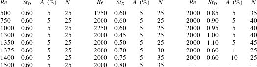
The list of all examined flow configurations is given in table 1; the influence of the Reynolds number, the Strouhal number and the forcing amplitude may thus be characterised. For high values of
 $St_{D}$
, a larger number of block-Arnoldi iterations are required in order to achieve convergence. Two competing time scales characterise the dynamics: the forcing period, which decreases with increasing
 $St_{D}$
, and the convection time, which is constant in all cases. Therefore, a constant number of iterations at high Strouhal number corresponds to a shorter convection time.
Absolute value of the dominant subharmonic Floquet multiplier for different
 $(Re,St_{D})$
, obtained for
 $A=5\,\%$
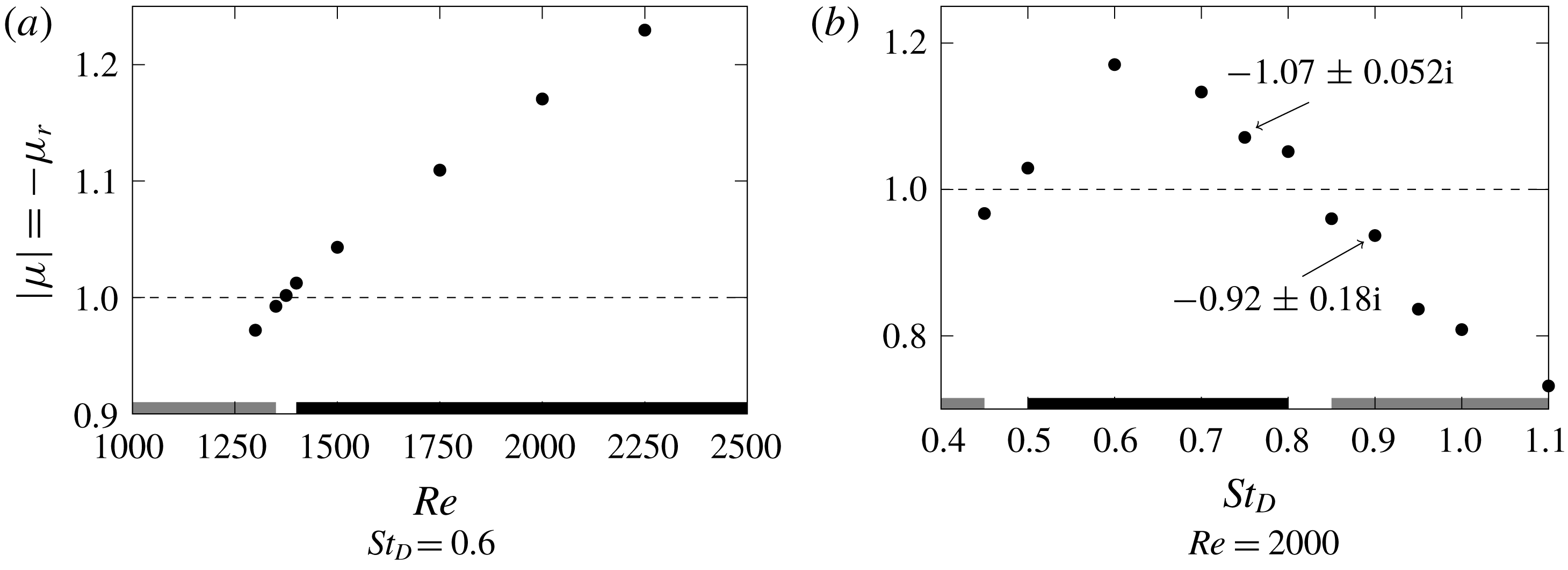
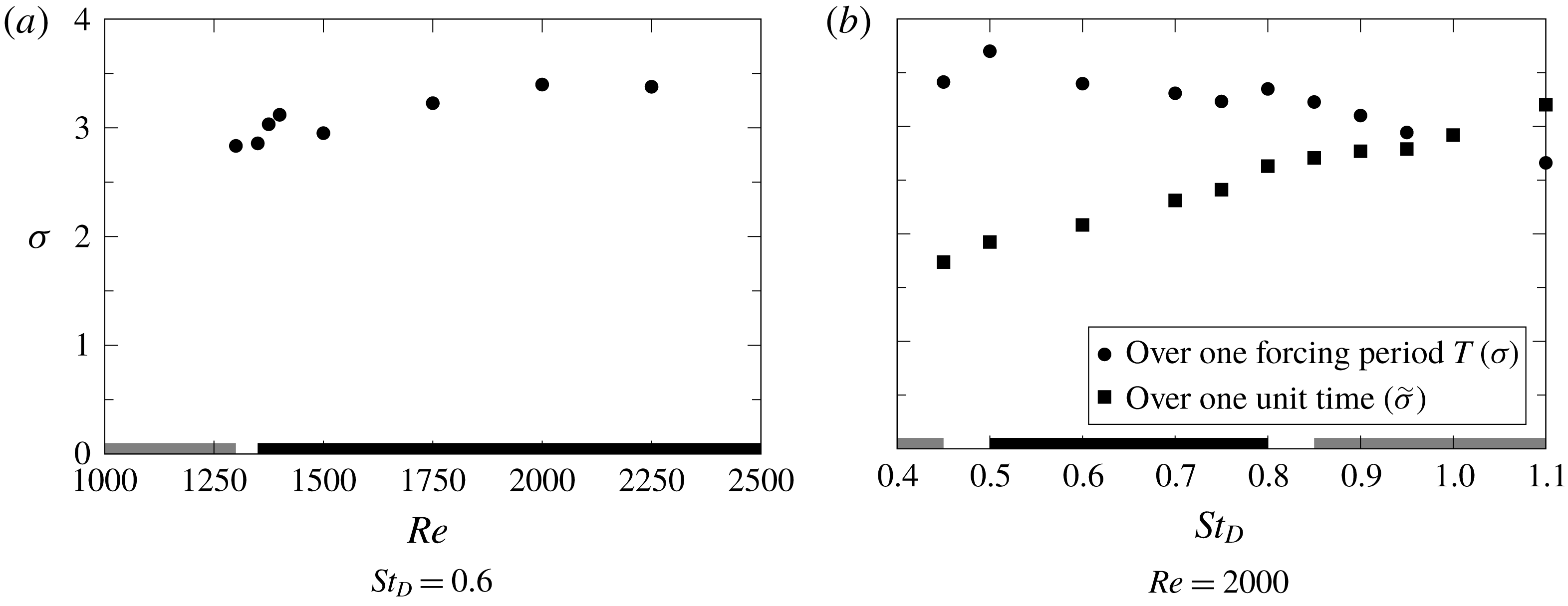
. When the system is unstable, the most unstable mode is always subharmonic (e.g. real negative), except for the two labelled cases in (b), where the most unstable mode is almost subharmonic. When the system is stable, the represented modes are the least stable of the subharmonic domain. Black and grey bars represent parameter regimes with and without vortex pairing, according to uncontrolled DNS (see figure 7).

Parameter combinations for which Floquet analysis is performed.

4.4 Floquet instability modes
As shown in table 1, nearly all calculations have been performed for constant forcing amplitude
 $A=5\,\%$
, and with fixed values of either
 $St_{D}=0.6$
or
 $Re=2000$
, in order to track the isolated influence of Strouhal and Reynolds number on the instability behaviour. In nearly all cases, one strictly subharmonic Floquet mode is identified, characterised by a negative real Floquet multiplier
 $\unicode[STIX]{x1D707}$
. This mode is observed to be unstable over certain ranges of
 $St_{D}$
and
 $Re$
, where
 $\unicode[STIX]{x1D707}$
falls below
 $-1$
. The absolute value
 $|\unicode[STIX]{x1D707}|=-\unicode[STIX]{x1D707}$
for
 $St_{D}=0.6$
and
 $A=5\,\%$
is plotted as a function of
 $Re$
in figure 13(a): by linear interpolation of the critical Reynolds at which
 $\unicode[STIX]{x1D707}_{c}=-1$
, instability in this case is found to arise for
 $Re\geqslant 1371$
. This is to be compared to the critical band
 $Re\in [1350;1400]$
, above (respectively below) which sustained pairing was found to occur (respectively not to occur) in the DNS, as discussed in § 3.4.1. The paired and unpaired regimes, as identified in the DNS, are indicated in figure 13(a) by black and grey bars, in order to highlight the agreement with the onset of subharmonic Floquet instability.
Results for variations in
 $St_{D}$
, at fixed values
 $Re=2000$
and
 $A=5\,\%$
, are presented in the same manner in figure 13(b). A finite band of subharmonically unstable Strouhal numbers is identified, again in agreement with the prevalence of vortex pairing as observed in the DNS. Two values of
 $\unicode[STIX]{x1D707}$
reported in this diagram are distinct from the others: at
 $St_{D}=0.75$
, the Floquet multiplier of the most unstable mode appears as a complex conjugate pair with small imaginary parts, as indicated in the figure. This mode is therefore nearly subharmonic, but not strictly so, and further iterations of the block-Arnoldi procedure do not change this result. Higher deviations from the negative real axis are found in the stable case
 $St_{D}=0.9$
. For
 $St_{D}=0.75$
, the unstable mode is slightly detuned, but the DNS does not display any irregular behaviour.
The effect of the forcing amplitude
 $A$
on the instability is demonstrated for a single setting
 $Re=2000$
and
 $St_{D}=0.6$
. As shown in table 2, a higher amplitude leads to stronger instability, consistent with the DNS observations discussed in § 3.4.2. Vortex pairing was found to occur in all three configurations.
Vorticity component of the most unstable Floquet mode at
 $Re=2000$
and
 $St_{D}=0.60$
. It peaks far downstream.

Evolution of the most unstable Floquet multiplier with the forcing amplitude for
 $Re=2000$
and
 $St_{D}=0.60$
.

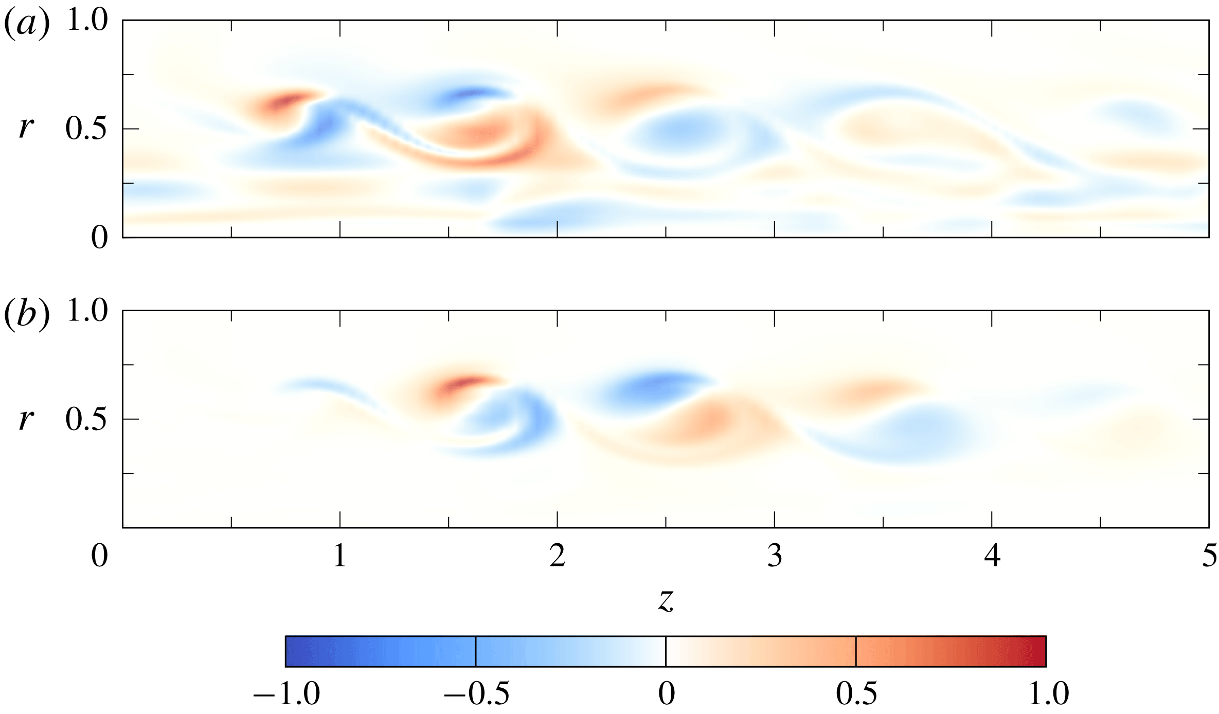
The spatial shape of an unstable subharmonic Floquet mode is presented in figure 14, for parameters
 $Re=2000$
,
 $St_{D}=0.6$
and
 $A=5\,\%$
, associated with
 $\unicode[STIX]{x1D707}=-1.17$
. A snapshot of perturbation vorticity is shown. Its axial wavelength corresponds to twice the spacing between vortices in the unpaired base flow, and its amplitude maximum occurs far downstream, around
 $z=20$
. The latter seems rather surprising, because the base flow vortices at this position are already quite diffuse, as can be seen in figure 3(c). Furthermore, vortex pairing in the unstabilised flow is observed around
 $z=3$
.
In order to demonstrate the effect of this modal shape on the unpaired base flow, the two are superposed, with a perturbation amplitude that is chosen ad hoc. The resulting vorticity field is shown in figure 15. It is seen that the perturbation indeed displaces the vortices around
 $z=20$
in a fashion that indicates pairing. This pattern was also found by Selçuk et al. (Reference Selçuk, Delbende and Rossi2017a
): the superposition of their quasi-static helical base flow and of their most unstable mode shows that their global mode shifts the helical vortices to trigger pairing.
Vorticity snapshot of the base periodic unpaired flow at
 $Re=2000$
and
 $St_{D}=0.6$
slightly perturbed by the most unstable Floquet mode:
 $\boldsymbol{u}^{\prime }=\boldsymbol{U}^{\boldsymbol{u}}+\unicode[STIX]{x1D716}\tilde{\boldsymbol{v}}_{1}$
, with
 $\unicode[STIX]{x1D716}=0.2$
.

However, in the current problem, the result from the superposition is very distinct from that of the fully developed paired state shown in figure 3(a). To explain this discrepancy, it might be speculated that nonlinear adjustments could occur, or that a different, non-dominant Floquet mode could be responsible for the onset of pairing. Indeed, a second unstable mode exists at this parameter setting, characterised by a Floquet multiplier value
 $-1.03\pm 0.14\text{i}$
, and its vorticity distribution is given in figure 16. It displays the same spatial pattern as the first Floquet mode, but shifted several diameters further downstream, and this shift presumably accounts for its weaker growth. As this mode is not strictly subharmonic, it does not evolve precisely at
 $\unicode[STIX]{x1D714}_{f}/2$
; still its growth may trigger subharmonic pairing in the nonlinear regime. However, this mode does not provide a more plausible interpretation of the observed vortex pairing much further upstream.
Real part of the vorticity component of the second most unstable Floquet mode at
 $Re=2000$
and
 $St_{D}=0.6$
. Its peak is located far downstream.

5 Transient growth analysis
In this section, we show that the transient dynamics is essential to understand the bifurcation from an unpaired unstable flow to a paired flow. Indeed, it will be demonstrated that even though the stability analysis predicts in which parameter range pairing occurs, the transition from an unpaired state arises much faster and much closer to the inlet that what modal theory predicts. In contrast, transient dynamics predicts more accurately the transition rate and the perturbation structures, and it allows us to explain the occurrence of intermittent phenomena in the sub-critical but noisy jets shown in § 3.4.3.
5.1 Growth of random initial perturbations
The jet at
 $Re=2000$
, forced at
 $St_{D}=0.6$
with 5 % amplitude is considered throughout this section. The natural state in this case is the paired one, shown in figure 7, consistent with an unstable Floquet multiplier
 $\unicode[STIX]{x1D707}=-1.17$
as discussed in § 4.4. Direct numerical simulation results are presented here, which aim to show how pairing is triggered in the unstable unpaired flow.
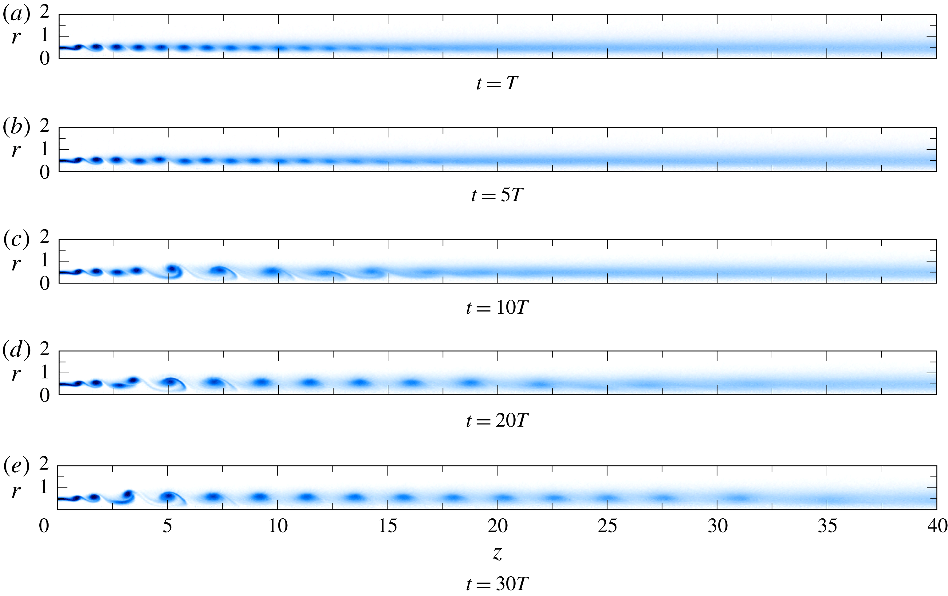
A first simulation is performed starting from the stabilised unpaired state, displayed in figure 3(c), as initial condition. Residual non-
 $T$
-periodic components
 $(u(t)-u(t-T))/2$
in this flow state are of the order of 0.01 % of the reference jet velocity.
Two additional simulations have been carried out with the same state, but with added white noise velocity perturbations,
 $\boldsymbol{u}(r,z,t=0)=\boldsymbol{U}^{\boldsymbol{u}}(r,z,t=0)+\unicode[STIX]{x1D750}(r,z)$
. This noise exhibits zero spatial mean
 $\overline{\unicode[STIX]{x1D750}}=\mathbf{0}$
, and two different standard deviations
 $\sqrt{\overline{\unicode[STIX]{x1D750}^{2}}}=(10^{-3},10^{-3})^{\mathit{T}}$
and
 $(10^{-4},10^{-4})^{\mathit{T}}$
are prescribed in the two simulations.
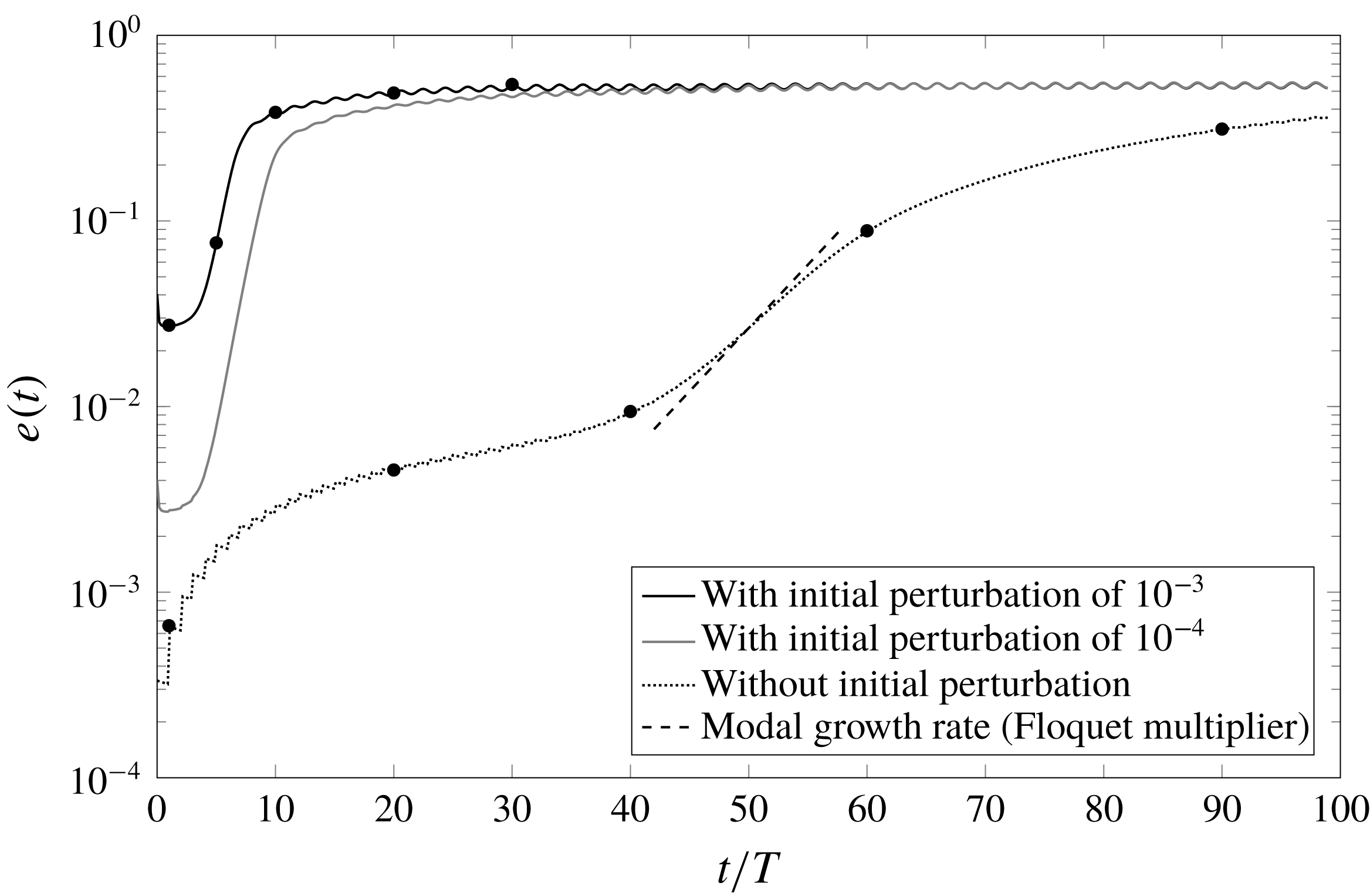
Non-harmonic components of the flow state at any given time are measured by a norm defined as
 $$\begin{eqnarray}e(t)=\frac{1}{2}\sqrt{\iint \Vert \boldsymbol{u}(t)-\boldsymbol{ u}(t-T)\Vert ^{2}r\,\text{d}r\,\text{d}z}.\end{eqnarray}$$
The time evolution of this norm is traced in figure 17 for the three different initial conditions. While all three cases evolve into the same paired attractor state, they arrive there along different trajectories.
Growth of non-harmonic components in simulations with and without added initial noise. The modal Floquet growth rate is indicated for comparison.

5.1.1 Modal growth from very low perturbation amplitude
Starting from the unpaired state, which has been obtained through flow stabilisation, without any added random noise, the initial perturbation that may give rise to a growing subharmonic component is given by the residual non-
 $T$
-periodicity that remained when the stabilised calculation was halted. The total vorticity after one period
 $T$
is shown in figure 18(a), and the magnitude of the non-
 $T$
-periodic residual at the same instant is presented in figure 19(a). Note that this residual is computed by comparing the state at time
 $t$
with that from time
 $t-T$
; therefore time stepping over one period is required before the stabilisation effect can be evaluated.
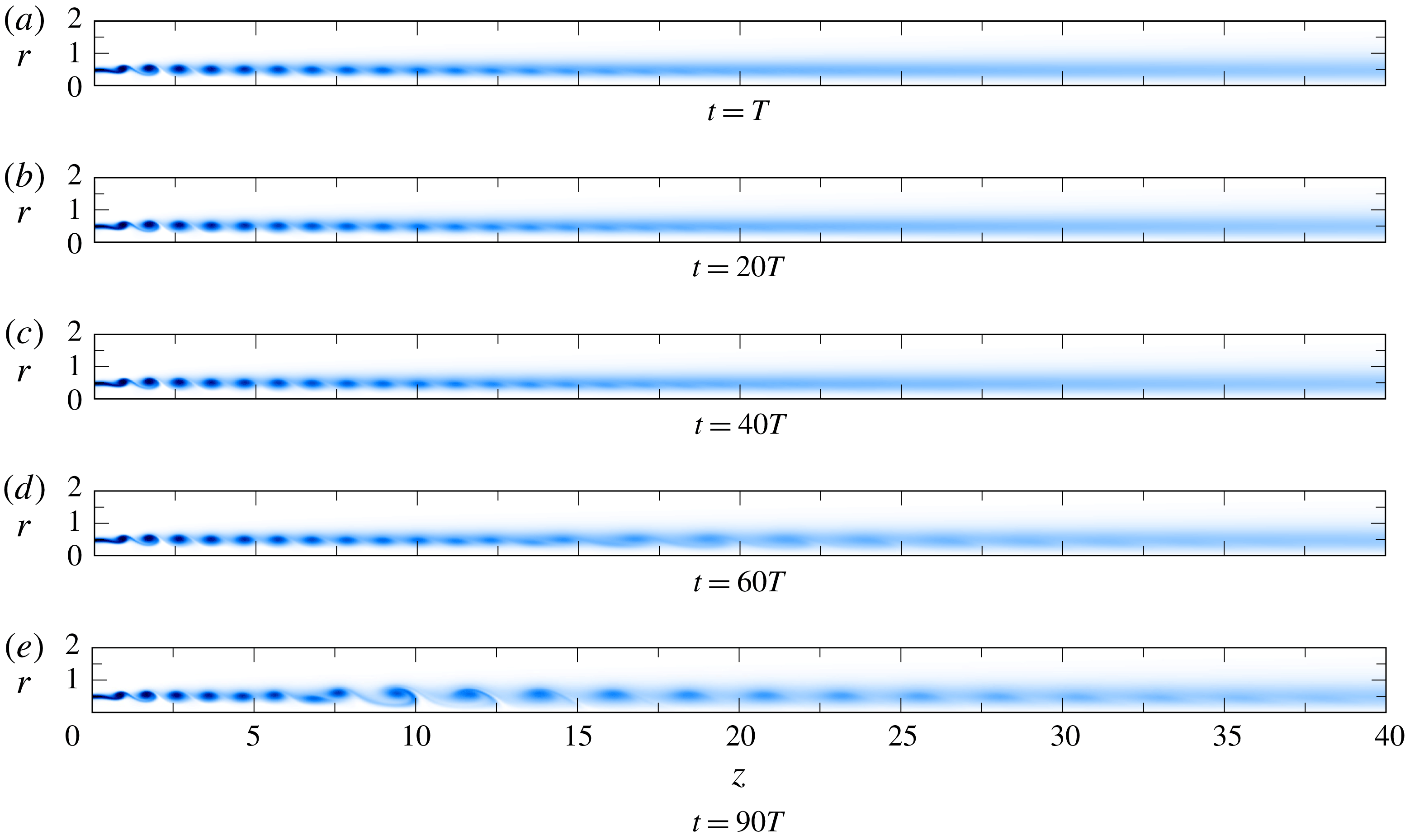
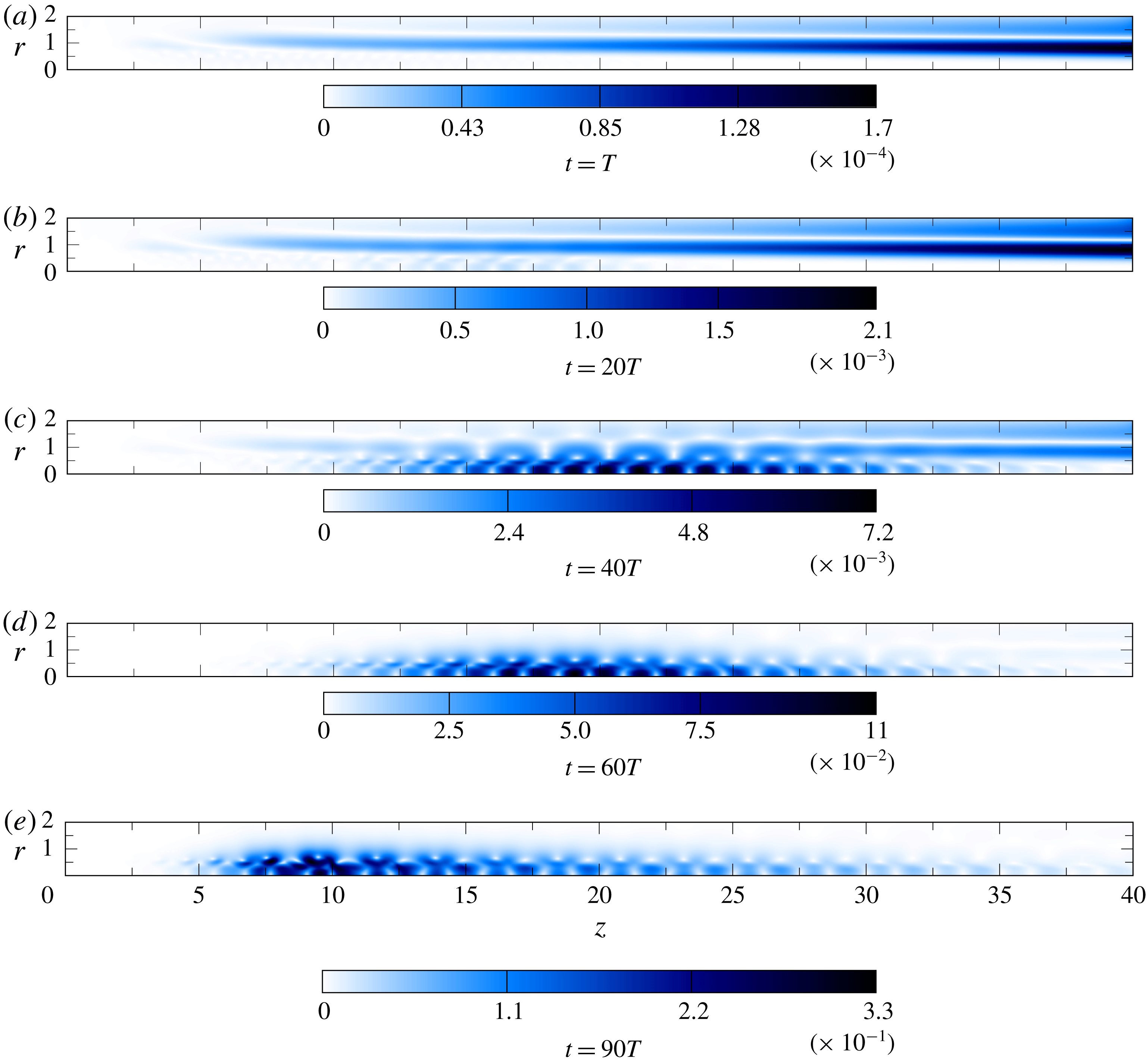
Over the first 40 periods, the subharmonic perturbation is dominated by a slow growth of the residual structure, but at such small amplitude that the total vorticity field in figure 18(b,c) is not noticeably affected. Then, as can be seen by comparing figures 19(c) and 19(d) with figure 14, the exponentially growing unstable Floquet mode becomes manifest. Its amplitude growth per flow period, between
 $t=40T$
and
 $60T$
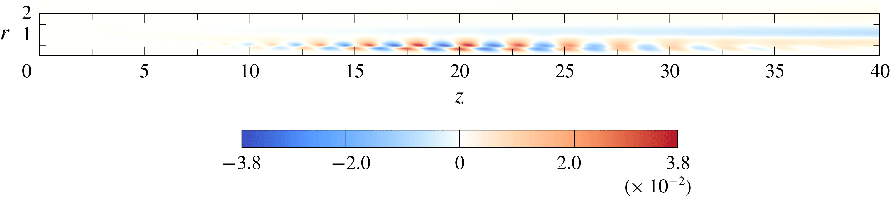
, is estimated from figure 17 as a factor 1.14, to be compared to the absolute value 1.17 of the computed Floquet multiplier. The spatial structure of this perturbation, displayed in figure 20, exhibits a similar structure as that of the corresponding Floquet mode, shown in figure 14. Beyond
 $t=60T$
, a nonlinear saturation of the subharmonic perturbation sets in (figure 17), accompanied by a change in its spatial shape. At
 $t=90T$
, as the flow approaches the asymptotic periodic regime, the maximum perturbation amplitude has moved upstream to
 $z\approx 10$
(figure 19
e), where a pronounced pairing of vortices is observed in figure 18(e). This pairing location still moves further upstream with time, until it will finally stabilise near
 $z=3$
, in the natural asymptotic paired state shown in figure 3(a).
Vorticity snapshots at five different instances without added initial noise. The colour coding is the same as in figure 3.

Perturbation magnitude
 $\Vert \boldsymbol{u}(t)-\boldsymbol{u}(t-T)\Vert$
at five different instances without added initial noise.

Vorticity field of the perturbation without any forcing applied at
 $t=40T$
.

5.1.2 Non-modal growth from initial white noise
The simulations with added white noise in the initial condition (solid lines in figure 17) show a much faster convergence to the final paired flow state than the case discussed in the preceding section (dotted line in figure 17). In particular, the initial growth of
 $e(t)$
in these two cases is markedly stronger than that of the unstable Floquet mode.
Five snapshots of vorticity, evolving out of initial white noise level
 $10^{-3}$
. The colour coding is the same as in figure 3(b).

The time development from an initial condition with
 $\sqrt{\overline{\unicode[STIX]{x1D750}^{2}}}=(10^{-3},10^{-3})^{\mathit{T}}$
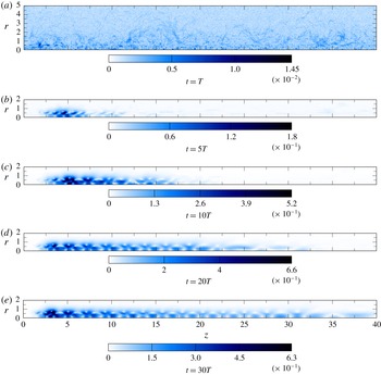
(thick solid line in figure 17) is visualised in figure 21 by successive snapshots of the total vorticity. It is seen that vortex pairing not only sets in faster than in the previous case of figure 18, but also much further upstream. Corresponding non-periodic perturbations are again displayed in figure 22: the smallest scales of the random initial condition are quickly dissipated (figure 22
a), and a growing coherent perturbation structure is evident after a few period cycles (figure 22
b). The maximum perturbation growth in this phase, as measured from figure 17, corresponds to a factor 2.01 per period, much stronger than the modal growth factor 1.17. Persistent vortex pairing is fully established at
 $t=10T$
(figure 22
c); subsequently, the pairing location slowly moves upstream, and stabilises around
 $z=3$
.
Vorticity perturbations after five flow periods, in these simulations with added initial noise, are represented in figure 23. At this early stage, their dynamics may still be regarded as linear; however, the perturbations are now located close to the inlet, and their spatial distribution bears no resemblance with the unstable Floquet mode (figure 14). Therefore, a non-modal mechanism is expected to underpin this growth.
Perturbation magnitude
 $\Vert \boldsymbol{u}(t)-\boldsymbol{u}(t-T)\Vert$
at five different instances evolving out of an initial white noise level
 $10^{-3}$
.

Vorticity field of the perturbation with random forcing (level
 $10^{-3}$
) at
 $t=5T$
.

Simulations with a lower initial noise level of
 $10^{-4}$
show a similar behaviour, although slightly delayed (figure 17). The exponential phase is longer, since the amplitude takes more time to saturate, and the maximum growth rate is 2.16 per forcing period.
In both the ‘unperturbed’ and ‘randomly perturbed’ cases, one should also note the absence of any sustained leap-frogging or overtaking events before pairing, contrary to what was observed by Selçuk et al. (Reference Selçuk, Delbende and Rossi2017a ). This can be understood because the jet vortex rings are much thicker compared their helical vortices, making leap-frogging and overtaking difficult.
5.2 Optimal linear perturbation growth over one cycle
In order to further analyse and understand the mechanism behind the non-modal onset of vortex pairing, as observed in § 5.1.2, the optimal growth of subharmonic perturbations is now investigated. One cycle period
 $T$
is chosen as the time horizon over which optimisation is performed. As discussed in the context of (4.6), perturbations are propagated over one cycle by the time-shift operator
 $\unicode[STIX]{x1D6F7}^{\prime }$
. The optimal perturbation is then found as the solution to the maximisation problem
 $$\begin{eqnarray}\Vert \boldsymbol{u}_{opt}(T)\Vert =\max _{\boldsymbol{u}^{\prime }(t=0)}\frac{\Vert \boldsymbol{u}^{\prime }(t=T)\Vert }{\Vert \boldsymbol{u}^{\prime }(t=0)\Vert }=\max _{\boldsymbol{u}^{\prime }(t=0)}\frac{\Vert \unicode[STIX]{x1D6F7}^{\prime }\boldsymbol{u}^{\prime }(t=0)\Vert }{\Vert \boldsymbol{u}^{\prime }(t=0)\Vert }.\end{eqnarray}$$
The norm used in the following is derived from the standard real
 $\boldsymbol{u}$
-scalar product in cylindrical coordinates (4.7). This scalar product defines a full norm for
 $\boldsymbol{u}$
, but only a semi-norm for
 $\boldsymbol{q}$
, because the separation condition is not fulfilled. The solution of the maximisation problem (5.2) is given by the norm of the operator
 $\unicode[STIX]{x1D6F7}^{\prime }$
.
To evaluate this norm, the orthonormal basis
 $\{\hat{\boldsymbol{u}}_{i}^{n}\}$
calculated in the context of modal analysis (§ 4.3) is once more exploited. Instead of maximising the norm of
 $\unicode[STIX]{x1D6F7}^{\prime }$
, a infinite-dimensional operator, we maximise the norm of its projection
 $\tilde{\unicode[STIX]{x1D6F7}}$
, of finite dimensions, onto this basis.
A perturbation state
 $\boldsymbol{u}^{\prime }$
is projected onto
 $\{\hat{\boldsymbol{u}}_{i}^{n}\}$
as
 $$\begin{eqnarray}\displaystyle & \displaystyle \boldsymbol{u}^{\prime }=\mathop{\sum }_{n=0}^{N-1}\mathop{\sum }_{i=1}^{N_{vec}}\unicode[STIX]{x1D737}_{nN_{vec}+i}\hat{\boldsymbol{u}}_{i}^{n}+\boldsymbol{r}^{\prime }, & \displaystyle\end{eqnarray}$$
 $$\begin{eqnarray}\displaystyle & \displaystyle \unicode[STIX]{x1D737}_{nN_{vec}+i}=\langle \boldsymbol{u}^{\prime },\hat{\boldsymbol{u}}_{i}^{n}\rangle \quad \text{such that }\unicode[STIX]{x1D737}=\unicode[STIX]{x1D64D}^{\text{T}}M\boldsymbol{u}^{\prime }. & \displaystyle\end{eqnarray}$$
The residual
 $\boldsymbol{r}^{\prime }$
is orthogonal to the basis
 $\{\hat{\boldsymbol{u}}_{i}^{n}\}$
, such that
 $\Vert \boldsymbol{u}^{\prime }\Vert ^{2}=\Vert \unicode[STIX]{x1D737}\Vert ^{2}+\Vert \boldsymbol{r}^{\prime }\Vert ^{2}$
. Therefore,
 $$\begin{eqnarray}\displaystyle \unicode[STIX]{x1D6F7}^{\prime }\boldsymbol{u}^{\prime } & = & \displaystyle \mathop{\sum }_{n=0}^{N-1}\mathop{\sum }_{i=1}^{N_{vec}}\unicode[STIX]{x1D737}_{nN_{vec}+i}(\unicode[STIX]{x1D6F7}^{\prime }\hat{\boldsymbol{u}}_{i}^{n})+\unicode[STIX]{x1D6F7}^{\prime }\boldsymbol{r}^{\prime }\end{eqnarray}$$
 $$\begin{eqnarray}\displaystyle & = & \displaystyle \mathop{\sum }_{n=0}^{N-1}\mathop{\sum }_{i=1}^{N_{vec}}(\tilde{\unicode[STIX]{x1D6F7}}\unicode[STIX]{x1D737})_{nN_{vec}+i}\hat{\boldsymbol{u}}_{i}^{n}+\unicode[STIX]{x1D6F7}^{\prime }\boldsymbol{r}^{\prime }\end{eqnarray}$$
and
 $$\begin{eqnarray}\Vert \unicode[STIX]{x1D6F7}^{\prime }\boldsymbol{u}^{\prime }\Vert ^{2}=\Vert \tilde{\unicode[STIX]{x1D6F7}}\unicode[STIX]{x1D737}\Vert ^{2}+\Vert \unicode[STIX]{x1D6F7}^{\prime }\boldsymbol{r}^{\prime }\Vert ^{2}+2\left\langle \mathop{\sum }_{n=0}^{N-1}\mathop{\sum }_{i=1}^{N_{vec}}(\tilde{\unicode[STIX]{x1D6F7}}\unicode[STIX]{x1D737})_{nN_{vec}+i}\hat{\boldsymbol{u}}_{i}^{n},\unicode[STIX]{x1D6F7}^{\prime }\boldsymbol{r}^{\prime }\right\rangle ,\end{eqnarray}$$
with the norm of
 $\tilde{\unicode[STIX]{x1D6F7}}\unicode[STIX]{x1D737}$
calculated in a finite-dimensional space of dimension
 $NN_{vec}$
. Therefore, maximising
 $\Vert \unicode[STIX]{x1D6F7}^{\prime }\boldsymbol{u}^{\prime }\Vert$
is equivalent to maximising the right-hand side of the previous equation. However, the
 $\hat{\boldsymbol{u}}_{i}^{n}$
-basis has not been chosen randomly: being constructed from the successive iterations of a single group of random vectors, it selects numerically the fastest-growing modes of the full system, in a similar way as power iterations (Saad Reference Saad2011). These modes are then gradually excluded from the residual space of
 $\boldsymbol{r}^{\prime }$
, and the norm of the image of
 $\boldsymbol{r}^{\prime }$
through
 $\unicode[STIX]{x1D6F7}^{\prime }$
decreases as the number
 $N$
of Krylov subspace iterations is increased. On the right-hand side of (5.7), the first term becomes dominant as
 $N$
increases; the second and third terms are bounded by
 $\Vert \unicode[STIX]{x1D6F7}^{\prime }\boldsymbol{r}^{\prime }\Vert ^{2}$
and
 $\Vert \tilde{\unicode[STIX]{x1D6F7}}\unicode[STIX]{x1D737}\Vert \Vert \unicode[STIX]{x1D6F7}^{\prime }\boldsymbol{r}^{\prime }\Vert$
, respectively. Therefore, the approximation
 $\Vert \unicode[STIX]{x1D6F7}^{\prime }\boldsymbol{u}^{\prime }\Vert \approx \Vert \tilde{\unicode[STIX]{x1D6F7}}\unicode[STIX]{x1D737}\Vert$
is valid for large
 $N$
. This explains why, for a given value of
 $NN_{vec}$
, a trade-off needs to be found between
 $N$
and
 $N_{vec}$
:
 $N$
must be large enough to capture the salient flow dynamics, whereas
 $N_{vec}$
must be sufficiently large to make the block-Arnoldi calculations computationally efficient.
The norm
 $\Vert \tilde{\unicode[STIX]{x1D6F7}}\unicode[STIX]{x1D737}\Vert$
is evaluated by use of the singular value decomposition (SVD)
 $$\begin{eqnarray}\tilde{\unicode[STIX]{x1D6F7}}=\tilde{\unicode[STIX]{x1D650}}\unicode[STIX]{x1D72E}\tilde{\unicode[STIX]{x1D651}}^{\text{T}},\end{eqnarray}$$
with
 $\unicode[STIX]{x1D72E}$
a real positive diagonal matrix, and
 $\tilde{\unicode[STIX]{x1D650}}$
and
 $\tilde{\unicode[STIX]{x1D651}}$
real unitary matrices. Columns
 $\tilde{\boldsymbol{v}}_{k}$
and
 $\tilde{\boldsymbol{u}}_{k}$
represent forcing and response pairs in the orthonormal basis of the
 $\{\hat{\boldsymbol{u}}_{i}^{n}\}$
;
 $\unicode[STIX]{x1D72E}$
contains the singular values ordered in descending order, such that
 $\tilde{\unicode[STIX]{x1D6F7}}\tilde{\boldsymbol{v}}_{k}=\unicode[STIX]{x1D70E}_{k}\tilde{\boldsymbol{u}}_{k}$
with
 $\unicode[STIX]{x1D70E}_{k}\geqslant \unicode[STIX]{x1D70E}_{k+1}\geqslant 0$
.
Note that the Krylov base constructed in § 4.3 is orthonormal with respect to the scalar product (4.7). Therefore, the optimal initial perturbations or responses in the reduced space correspond to the optimal initial perturbations or responses in the full-state space, using the
 $\unicode[STIX]{x1D64D}$
matrix to change basis. For a given optimal initial perturbation (respectively response)
 $\tilde{\boldsymbol{v}}_{k}$
(respectively
 $\tilde{\boldsymbol{u}}_{k}$
) in this reduced basis, the corresponding full-state initial perturbation velocity (respectively response velocity)
 $\boldsymbol{v}_{k}$
(respectively
 $\boldsymbol{u}_{k}$
) is obtained as
 $\boldsymbol{v}_{k}=\unicode[STIX]{x1D64D}\tilde{\boldsymbol{v}}_{k}$
(respectively
 $\boldsymbol{u}_{k}=\unicode[STIX]{x1D64D}\tilde{\boldsymbol{u}}_{k}$
). The corresponding matrices of optimal initial perturbations and responses are
 $\unicode[STIX]{x1D651}=\unicode[STIX]{x1D64D}\tilde{\unicode[STIX]{x1D651}}$
and
 $\unicode[STIX]{x1D650}=\unicode[STIX]{x1D64D}\tilde{\unicode[STIX]{x1D650}}$
. Because of this preserved optimality, the maximum linear gain achievable over one period in the full state is still
 $\unicode[STIX]{x1D70E}_{1}$
, obtained by perturbing the velocity field at
 $t=0$
with
 $\boldsymbol{v}_{1}$
. After one period, the perturbation velocity field is given by
 $\boldsymbol{u}_{1}$
.
This method is computationally efficient, as it is entirely based on the results already available from the modal analysis. This is in contrast with the additional computations required in a direct–adjoint approach. Moreover, with the direct–adjoint approach, the optimisation is carried out for a single time horizon
 $T_{f}$
. In this section, only
 $T_{f}=T$
has been chosen; however, as will be seen in the next section, this can be extended with little additional effort to any time horizon of integer period
 $T_{f}=nT$
. Time horizons that are not integer multiples of
 $T$
, corresponding to transient phenomena within a forcing period, are not considered here.
Singular value decomposition of
 $\unicode[STIX]{x1D6F7}^{\prime }$
has been carried out for all flow configurations listed in table 1. The maximum gain values
 $\unicode[STIX]{x1D70E}_{1}$
are shown in figure 24 for fixed values of
 $St_{D}$
and
 $Re$
. Variations of
 $\unicode[STIX]{x1D70E}_{1}$
with the forcing amplitude
 $A$
are given in table 3 for one setting
 $Re=2000$
and
 $St_{D}=0.6$
. In all cases, the achievable transient amplification over one period is significantly higher than the maximum modal growth rate. A comparison with results of perturbed DNS flows (figure 17) is discussed in § 5.3.
Norm of the time-shift operator for different Reynolds and Strouhal numbers, with a 5 % forcing level and a normalised momentum thickness of 5 %. The grey or black domains represent the parameter values for which DNS calculations show that the ‘natural’ solution is unpaired or paired, as shown in figure 7. In (b), the leading amplification rates are also depicted rescaled over one dimensionless time unit. Additional singular values for lower Reynolds number flows are discussed in § 5.4.

Evolution of the optimal perturbation gain over one period with the forcing amplitude for
 $Re=2000$
and
 $St_{D}=0.60$
.

At fixed Strouhal number (figure 24
a), the leading singular value changes weakly as a function of Reynolds number, even as the system goes from stable to unstable. Variations of
 $\unicode[STIX]{x1D70E}_{1}$
are within 20 % as the value of
 $Re$
is doubled.
At fixed Reynolds number (figure 24
b), variations of the Strouhal number also do not affect
 $\unicode[STIX]{x1D70E}_{1}$
in a strong way. Doubling
 $St_{D}$
from 0.45 to 0.9 is accompanied by a 10 % decrease of the maximum gain over one flow period. However, when
 $\unicode[STIX]{x1D70E}_{1}$
is rescaled to give the mean amplification over a constant time unit, as
 $\tilde{\unicode[STIX]{x1D70E}}_{1}=\unicode[STIX]{x1D70E}_{1}St_{D}$
, this rescaled gain increases by more than 30 % over the investigated interval of
 $St_{D}$
. This is consistent with Broze & Hussain (Reference Broze and Hussain1994, Reference Broze and Hussain1996): in their parametric study, as shown in figure 2, they found that when the Strouhal number is increased, the jet is more prone to experience non-
 $T$
- or non-
 $2T$
-periodic behaviour (periodic or not modulations, intermittency or chaos). Our study shows that the larger the Strouhal number, the more amplified random perturbations can be over a given time unit.
With increasing forcing amplitude, the maximum gain is moderately diminished (table 3). This may indicate that the receptivity to subharmonic perturbations is larger when the shear layer is not yet fully rolled up, since increasing forcing amplitude results in a faster roll-up of vortices, as shown in figure 9. Again, this is coherent with Broze & Hussain (Reference Broze and Hussain1994, Reference Broze and Hussain1996): as shown in figure 2, with larger forcing levels, except at Strouhal numbers greater than those considered in our study, the flow is less prone to non-periodic behaviour, which may be brought about by transient amplification of small disturbances.
The leading singular mode may not be the only relevant way to trigger transient growth. For the case
 $(Re=2000,St_{D}=0.6)$
, the 20 largest singular values are represented in figure 25. Indeed, a strong dominance of the optimal perturbation cannot be affirmed: the first value is 15 % larger than the second, 27 % larger than the third, and only 87 % larger than the twentieth.
The twenty largest singular values of
 $\unicode[STIX]{x1D6F7}^{\prime }$
for
 $Re=2000$
,
 $St_{D}=0.6$
and
 $A=5\,\%$
.

The shapes of the optimal initial perturbation and response structures are shown for the case
 $(Re=2000,St_{D}=0.6)$
in figures 26(a) and 26(b), respectively. In comparison with the Floquet mode discussed in § 4.4 (see figure 14), these perturbation structures are localised much closer to the inlet. Over the course of one period, the perturbation shape is largely conserved, while it is convected at the same pace as the rolled-up vortices. The manifestation of these perturbations in the total vorticity field is visualised in figure 27, where the linear optimal initial perturbation and response structures are superposed onto the periodic base state with a small amplitude of 5 %. It can be observed that the optimal perturbation structures displace the vortices towards and away from the axis, in an alternating fashion. This displacement is furthermore oriented at an oblique angle, such that the distance between neighbouring vortices is modulated, thus initiating the pairing interaction.
For
 $Re=2000$
and
 $St_{D}=0.6$
, vorticity of (a) the optimal perturbation and (b) its response after one flow period. The maxima are located close to the inlet.

Superposition of the base flow and (a) the optimal perturbation, (b) the associated linear response after one flow period. The total vorticity is shown, for velocity fields
 $\boldsymbol{u}^{\prime }=\boldsymbol{U}^{\boldsymbol{u}}+0.05\boldsymbol{u}_{\mathbf{1}}$
and
 $\boldsymbol{u}^{\prime }=\boldsymbol{U}^{\boldsymbol{u}}+0.05\unicode[STIX]{x1D70E}_{1}\boldsymbol{v}_{\mathbf{1}}$
, respectively, for the case
 $Re=2000$
and
 $St_{D}=0.6$
. Both
 $\boldsymbol{u}_{\mathbf{1}}$
and
 $\boldsymbol{v}_{\mathbf{1}}$
have unit norm.

The second singular mode pair in the same configuration, corresponding to
 $\unicode[STIX]{x1D70E}_{2}$
, is displayed in figure 28. It exhibits a very similar structure as the first singular mode, the main difference being that the maximum amplitude is shifted downstream to the next vortex pair.
For
 $Re=2000$
and
 $St_{D}=0.6$
, vorticity of the second singular mode: (a) perturbation and (b) its response after one flow period. The maxima are located further downstream than in the optimal setting shown in figure 26.

Transient growth gain achieved by a
 $(Re=2000,St_{D}=0.60)$
jet forced with 5 % amplitude and comparison with modal growth.

5.3 Optimal linear perturbation growth over many cycles
The technique that has been described in the previous section for optimisation over a single flow period
 $T$
is easily extended in order to construct optimal perturbations for time horizons of multiple periods
 $nT$
. Let
 $\boldsymbol{f}_{n}$
denote the optimal perturbation at
 $t=0$
that leads to the largest possible flow response
 $\boldsymbol{r}_{n}$
at
 $t=nT$
. The associated amplitude gain is then given by the norm
 $\Vert \boldsymbol{u}_{opt}(nT)\Vert =\Vert \boldsymbol{r}_{n}\Vert /\Vert \boldsymbol{f}_{n}\Vert$
, which is identical to the largest singular value of the
 $n$
th power of the operator
 $\unicode[STIX]{x1D6F7}$
. Substituting
 $\unicode[STIX]{x1D6F7}$
with its approximation
 $\tilde{\unicode[STIX]{x1D6F7}}$
, the SVD of
 $\tilde{\unicode[STIX]{x1D6F7}}^{n}$
is straightforward to compute.
The ensuing variation of the optimal gain with
 $nT$
is traced in figure 29, alongside the perturbation growth associated with the most unstable Floquet mode (§ 4.4). Optimal perturbation at
 $t=0$
enables a vigorous transient growth over short time horizons; at longer times, however, the optimal growth rate approaches that of the modal solution, given by the modulus of the dominant Floquet multiplier. This behaviour is identical to that of perturbation growth in steady base flows, which has been discussed theoretically by Trefethen & Embree (Reference Trefethen and Embree2005). In the present case, the transient non-modal growth provides a significant boost, of the order of
 $10^{5}$
, of the overall long-time amplitude gain. This additional factor corresponds to 73 cycle periods of modal growth.
The evolution and convergence of the optimal initial perturbation and response structures are examined in figure 30 in terms of projections. The scalar products of the initial perturbation and response structures obtained for any number of cycles with those at
 $n=1$
and
 $n=50$
are represented. It is observed that the optimal initial perturbation structure does not evolve much with time, and that the shape determined for one single period is close to optimality for all time horizons. In contrast, the shape of the optimal response changes significantly through time; the optimal response at
 $t=50T$
is indeed localised at a different location than its counterpart at
 $t=T$
. While the optimal initial perturbation structure always retains a nearly identical shape, the optimal response structure gradually shifts downstream with increasing time horizon, and eventually it converges towards the structure of the Floquet mode (see figure 14). The projection values in table 4 demonstrate this convergence. It is expected on theoretical grounds (Trefethen & Embree Reference Trefethen and Embree2005) that, at long-time horizons, the optimal response structure corresponds to the dominant Floquet mode, whereas the optimal forcing is given by the associated adjoint mode of the time-shift operator.
Projection of the optimal initial perturbation and response at time
 $nT$
over the optimal initial perturbation and responses at times
 $T$
and
 $50T$
for a jet at
 $Re=2000$
and
 $St_{D}=0.60$
forced with a 5 % amplitude. While the optimal initial perturbation experiences little change, the optimal response changes drastically. All vectors considered have unit norm.

Scalar products (4.7) between the Floquet mode
 $\tilde{\boldsymbol{v}}_{1}$
and the optimal finite-time initial perturbations
 $\boldsymbol{f}_{n}$
and responses
 $\boldsymbol{r}_{n}$
. All modes and perturbations have unit norm. Consistent with the notations introduced in § 5.2,
 $\boldsymbol{f}_{1}$
is identical to
 $\boldsymbol{v}_{1}$
, and
 $\boldsymbol{r}_{1}$
to
 $\boldsymbol{u}_{1}$
.

The different evolution from different initial perturbations, documented in §§ 5.1.1 and 5.1.2, can now be interpreted in terms of the optimal perturbation results.
In the two cases that were initialised with white noise perturbations, this initial condition contained significant components of strongly amplified optimal initial perturbation modes. After approximately five periods, these structures emerged from the background noise, as may be inferred from a qualitative comparison between figures 23, 26(b) and 28(b). However, the maximum growth observed in figure 17 for
 $\sqrt{\overline{\unicode[STIX]{x1D750}^{2}}}=(10^{-3},10^{-3})^{\mathit{T}}$
corresponds to a factor 2.16 per period, whereas the leading singular value was determined to be 3.40 in § 5.2 for the time horizon
 $t=T$
. Yet, the optimal growth rate decreases with time; this is shown in figure 31, which represents the marginal gain
 $\unicode[STIX]{x1D70E}_{m}(nT)$
at
 $t=nT$
of the
 $nT$
-optimal perturbation:
 $$\begin{eqnarray}\unicode[STIX]{x1D70E}_{m}(nT)=\frac{\Vert \boldsymbol{u}_{opt}[(n+1)T]\Vert }{\Vert \boldsymbol{u}_{opt}(nT)\Vert },\end{eqnarray}$$
with
 $\Vert \boldsymbol{u}_{opt}(nT)\Vert$
plotted in figure 29. Therefore, the maximum growth value 2.16, observed in figure 17, is consistent with the marginal gains observed after 5 to 10 periods in figure 31.
Marginal gain
 $\unicode[STIX]{x1D70E}_{m}(nT)$
of the optimal perturbation at the horizon time
 $nT$
for
 $Re=2000$
,
 $St_{D}=0.60$
and
 $A=0.05$
. The marginal growth rate asymptotically converges towards the modulus of the most unstable Floquet multiplier.

In the case discussed in § 5.1.1, initialised without added noise, the exponential growth observed between
 $40T$
and
 $60T$
has been associated with the unstable Floquet mode. The initial perturbation (figure 19
a) is spatially disjoint from optimal perturbations near the inflow. At
 $t=20T$
, a non-modal pairing perturbation is faintly visible in figure 19(b), still in the process of transitioning towards the Floquet mode in figure 19(c), the optimal linear response at long times.
Whether or not transient processes lead to a rapid onset of nonlinear vortex pairing depends on the energy level of oscillatory perturbations near the inflow, with appropriate wavelengths for subharmonic vortex modulation.
5.4 Importance of transient dynamics at low
$Re$

In § 3.4.1, a Reynolds number threshold was determined below which pairing no longer occurred naturally. However, in § 3.4.3, it has been demonstrated that forcing a jet harmonically with a small noise level was able to trigger pairing for Reynolds numbers where pairing does not normally occur. It is now examined how this behaviour can be explained in the light of the transient growth analysis developed in the previous section. At
 $St_{D}=0.6$
and
 $A=5\,\%$
, four Reynolds number values 1300, 1000, 750 and 500 are considered here. All these cases are modally stable, as seen in table 5. The transient growth of these cases is shown in figure 32.
Although in all cases, the gain decreases in the long term, the maximum achieved during the transient growth varies largely, between 4.5 after 6 periods for
 $Re=500$
, and
 $8.3\times 10^{3}$
after 26 periods for
 $Re=1300$
. This change explains the different behaviour observed in § 3.4.3. At
 $Re=500$
, whatever the forcing level, the noise is not energetic enough to trigger pairing. On the other hand, at
 $Re=1300$
, even very small perturbations eventually initiate pairing via transient growth. At intermediate Reynolds numbers, the behaviour observed depends on the perturbation level.
Transient growth gain for a jet forced at
 $St_{D}=0.60$
with 5 % amplitude at different subcritical Reynolds number values.

For
 $St_{D}=0.6$
and
 $A=0.05$
, evolution of the least stable subharmonic Floquet multiplier and of the maximum growth rate over one period as a function of
 $Re$
in the stable case.

6 Conclusion
The onset of sustained vortex pairing in the street of axisymmetric vortices in a laminar jet has been investigated by means of global instability analysis.
The numerical framework developed for this study is applicable to the instability analysis of any spatially developing time-periodic flow. It includes the computation of a strictly
 $T$
-periodic base flow by means of DNS with added time-delay control (Shaabani-Ardali et al.
Reference Shaabani-Ardali, Sipp and Lesshafft2017), the identification of dominant linear Floquet modes and a singular value decomposition of the propagator in order to characterise non-modal transient growth phenomena. The modal and non-modal analysis are both achieved via time stepping of the linearised flow equations, without the need for adjoint calculations, in combination with a block-Arnoldi algorithm (Saad Reference Saad2011).
It has been demonstrated that self-sustained vortex pairing in a jet is the manifestation of a subharmonic linear Floquet instability of the underlying periodic vortex street. Direct numerical simulations of axisymmetric laminar jets, forced harmonically at Strouhal number
 $St_{D}$
at the inlet, have been performed in order to delineate the region in the (
 $Re,St_{D}$
) parameter plane where pairing in the ensuing vortex street arises spontaneously. This parameter regime has then been shown to be characterised by subharmonic Floquet instability. Furthermore, the phase velocities of fundamental and subharmonic fluctuations in the simulation results have been found to be consistent with the resonance model proposed by Monkewitz (Reference Monkewitz1988). DNS results also show a strong influence of inflow forcing amplitude as well as random ambient noise on the onset of vortex pairing.
The spatial structure of the unstable linear Floquet mode, throughout the parameter regime considered in this study, reaches its maximum amplitude far downstream of the inlet, whereas the subharmonic perturbation amplitude in the nonlinear saturated paired flow state peaks a few diameters away from the inlet, where stationary vortex pairing occurs. When DNS calculations in the unstable regime are initiated with extremely low subharmonic perturbations, the Floquet mode structure and growth rate are indeed observed over a short time interval in the bifurcation process. However, when additional random noise is added to the initial condition, considerably faster subharmonic perturbation growth is observed, with spatial amplitudes concentrated near the inlet. This behaviour motivated a linear optimal perturbation analysis. It has been found that linear transient mechanisms may induce, for a standard configuration with
 $Re=2000$
and
 $St_{D}=0.6$
, an additional amplitude gain of approximately five orders of magnitude with respect to purely modal growth. Furthermore, the spatial structure of the linear optimal perturbation response reflects the DNS observations at early times, when subharmonic perturbations may be assumed to be governed by linear dynamics.
While the asymptotic occurrence of vortex pairing is determined by modal Floquet instability, its emergence is dominated by non-modal transient growth mechanisms.
Acknowledgements
We thank H. Johnson for her help with Nek5000 and R. Yegavian for his help with the parallelisation of FreeFem
 $++$
. This work was granted access to the HPC resources of TGCC under the allocation grant no. 2016-2a6451 made by GENCI, and it was financially supported by the Délégation Générale de l’Armement under grant no. 2015.60.0004.00.470.75.01.