
 B



1. Introduction
Jet noise remains a challenging prediction problem because the radiated sound energy emerges from a multiscale turbulent flow in which only a limited part of the unsteady motion is acoustically efficient. A central issue, therefore, is not to describe the turbulence itself, but to identify the flow structures and source mechanisms that make the dominant contribution to far-field sound. Over the years, this has motivated a wide range of analysis and modelling strategies. These have been based on acoustic analogies (Lighthill Reference Lighthill1952; Lilley Reference Lilley1974; Goldstein Reference Goldstein2003), on instability-wave models (Goldstein & Leib Reference Goldstein and Leib2005; Cavalieri et al. Reference Cavalieri, Rodríguez, Jordan, Colonius and Gervais2013; Jordan & Colonius Reference Jordan and Colonius2013; Sinha et al. Reference Sinha, Rodríguez, Brès and Colonius2014) and most recently on resolvent-based formulations (Cavalieri et al. Reference Cavalieri, Jordan and Lesshafft2019; Lesshafft et al. Reference Lesshafft, Semeraro, Jaunet, Cavalieri and Jordan2019; Karban et al. Reference Karban, Bugeat, Towne, Lesshafft, Agarwal and Jordan2023; Bugeat et al. Reference Bugeat, Karban, Agarwal, Lesshafft and Jordan2024). When formulated for aeroacoustic problems, resolvent analysis provides a frequency-domain, discrete counterpart to classical aeroacoustic integral formulations, allowing old problems to be revisited through the lens of linear algebra. The present work applies this framework to the problem of jet-noise modelling.
From the first acoustic analogy (Lighthill Reference Lighthill1952) to the most recent (Goldstein Reference Goldstein2003), the study of sound generation by turbulence has been anchored in linearisations of the flow equations, with nonlinear effects aggregated in an endogenous, inhomogeneous source term. These exact reorganisations of the Navier–Stokes system have provided frameworks for simplified sound-source modelling which have been instrumental in clarifying the acoustic importance of (experimentally observed) coherent structures in turbulent jets (Crow Reference Crow1972; Ffowcs-Williams & Kempton Reference Ffowcs-Williams and Kempton1978; Cavalieri et al. Reference Cavalieri, Jordan, Colonius and Gervais2012; Cavalieri & Agarwal Reference Cavalieri and Agarwal2014). Acoustic matching, discussed in early studies (Lighthill Reference Lighthill1952; Ffowcs-Williams Reference Ffowcs-Williams1963; Crighton Reference Crighton1975), is a central idea: only those source scales compatible with the dispersion relation of the linear operator can radiate sound. While each linear operator (for each acoustic analogy) has an associated, unique dispersion relation, all linearised formulations to date indicate the same basic requirement for a source term to be acoustically effective: some part of the source field must have sonic phase speed in the propagation direction. One may compare, for instance, the discussion of acoustic matching by Crighton (Reference Crighton1975), where physical interpretation is based on the d’Alembertian, with those of Goldstein (Reference Goldstein2005), Garnaud et al. (Reference Garnaud, Sandberg and Lesshafft2013), Jeun et al. (Reference Jeun, Nichols and Jovanović2016) or Bugeat et al. (Reference Bugeat, Karban, Agarwal, Lesshafft and Jordan2024), all four of which are based on linearisation about a spatially evolving shear flow. Acoustic matching has, furthermore, provided a framework for analysis, post-processing and modelling strategies over the years (Freund Reference Freund2001; Goldstein Reference Goldstein2003, Reference Goldstein2005; Cabana et al. Reference Cabana, Fortuné and Jordan2008; Tinney & Jordan Reference Tinney and Jordan2008; Sinayoko et al. Reference Sinayoko, Agarwal and Hu2011; Karban et al. Reference Karban, Bugeat, Towne, Lesshafft, Agarwal and Jordan2023).
When linearisation is performed about a shear flow, the operator describes, in addition to the convection and refraction of sound by velocity gradients, the amplification mechanisms that underpin coherent structures (wavepackets) (Jordan & Colonius Reference Jordan and Colonius2013; Cavalieri et al. Reference Cavalieri, Jordan and Lesshafft2019). These amplification mechanisms are most clearly revealed when the linear operator is considered in resolvent form (Cavalieri et al. Reference Cavalieri, Jordan and Lesshafft2019; Lesshafft et al. Reference Lesshafft, Semeraro, Jaunet, Cavalieri and Jordan2019; Nogueira et al. Reference Nogueira, Cavalieri, Schmidt, Jordan, Jaunet, Pickering, Rigas and Colonius2019; Pickering et al. Reference Pickering, Rigas, Nogueira, Cavalieri, Schmidt and Colonius2020; Maia et al. Reference Maia, Brès, Lesshafft and Jordan2023, Reference Maia, Heidt, Pickering, Colonius, Jordan and Brès2024). Agreement between coherent structures so modelled and those educed from experimental and numerical data is compelling over a broad range of frequencies and azimuthal wavenumbers, both for jets in static ambient conditions (Pickering et al. Reference Pickering, Rigas, Nogueira, Cavalieri, Schmidt and Colonius2020) and in the presence of a flight stream (Maia et al. Reference Maia, Brès, Lesshafft and Jordan2023, Reference Maia, Heidt, Pickering, Colonius, Jordan and Brès2024). The results also show that turbulent jets are predominantly populated by three basic kinds of coherent structures, each underpinned by a specific instability mechanism (Kelvin–Helmholtz, Orr, lift-up) (Pickering et al. Reference Pickering, Rigas, Nogueira, Cavalieri, Schmidt and Colonius2020).
In aeroacoustics, resolvent analysis involves the frequency space linear operator by which source and sound are connected. Once discretised, the operator is a matrix that can be used to numerically compute the sound field given the source field: from the inhomogeneous differential linear system
 $L\hat {p}=\hat {s}$
, one obtains the integral system
 $\hat {p}=R\hat {s}$
, where
 $L$
is the linear operator,
 $R=L^{-1}$
is the resolvent operator, and
 $\hat {p}$
and
 $\hat {s}$
are the complex Fourier amplitudes of sound pressure and source, respectively. So formulated, one has a discrete, matrix representation of the Green’s function solutions traditionally considered in integral aeroacoustics problems. The action of the resolvent operator on the source is, as mentioned above, nothing other than a discrete, frequency space representation of the action of the Green’s function in aeroacoustic integral methods.
A novel feature of resolvent analysis, compared with the standard Green’s function approach, is the use of the singular-value decomposition (SVD),
 $\hat {p}=U \! \varSigma V^H \hat {s}$
, which provides orthonormal input and output-vector bases,
 $U$
and
 $V$
, respectively, that rank the gains between inputs and outputs through the corresponding singular values contained in the diagonal matrix,
 $\varSigma$
. When the singular values decay rapidly, truncating the SVD provides reduced-rank approximations of the full solution.
With a so-called acoustic formulation of the resolvent problem, where the underpinning optimality problem searches for source modes that maximise an acoustic output, the gain matrix does not always decay rapidly (Garnaud et al. Reference Garnaud, Sandberg and Lesshafft2013; Jeun et al. Reference Jeun, Nichols and Jovanović2016; Bugeat et al. Reference Bugeat, Karban, Agarwal, Lesshafft and Jordan2024). One must therefore consider the source field in detail to understand its projection onto the input-vector space. Cast in a two-point framework,
 $\langle \hat {p}\hat {p}^*\rangle =U\varSigma V \langle \hat {s}\hat {s}^*\rangle V\varSigma U^H$
, we see that power- and cross-spectral densities of the sound field, contained in the cross-spectral density (CSD),
 $\langle \hat {p}\hat {p}^*\rangle$
, are driven by the CSD of the source field,
 $\langle \hat {s}\hat {s}^*\rangle$
, via the resolvent operator.
As the source in an acoustic analogy is nonlinear in the turbulence velocity fluctuations, the object of interest, its CSD, is a large, high-rank matrix, associated with two-point, fourth-order statistics. It is a formidably difficult object to compute or measure. To understand the acoustic-matching phenomena by which a high-rank source field produces a low-rank sound field, methodologies are required that would provide access to the part of the CSD that dominates the projection, or a simplified model of this. If that can be identified, simplified sound-source modelling strategies can be elaborated based on the acoustically active scales of the turbulence.
Based on methodologies developed to educe and model coherent structures in incompressible shear-flow problems (Martini et al. Reference Martini, Cavalieri, Jordan, Towne and Lesshafft2020; Towne et al. Reference Towne, Lozano-Durán and Yang2020; Karban et al. Reference Karban, Martini, Cavalieri, Lesshafft and Jordan2022b ), Karban et al. (Reference Karban, Bugeat, Towne, Lesshafft, Agarwal and Jordan2023) addressed the jet-noise problem with the goal of identifying the acoustically active part of the source CSD in a Mach 0.9 turbulent jet. It was necessary to compute the source CSD from high-fidelity numerical simulation, run for many thousands of convective time units. Specially developed signal-processing techniques were required to address aliasing issues (Karban et al. Reference Karban, Martini, Jordan, Brès and Towne2022), and a dedicated modal decomposition tool, resolvent-based-extended-spectral proper orthogonal decomposition (RESPOD), was developed to obtain a low-rank approximation of the acoustically matched source structure. On the basis of the RESPOD result, a rank-1 empirical model was proposed and shown to capture the effect of variations of jet and flight-stream Mach number.
This difficulty of identifying sound-source activity from turbulent flow motivates the development of sound-source identification methodologies that use data acquired in the sound field to infer the structure of the source. Such techniques have been applied to jets over the years, in various forms (cf. Fisher & Holland Reference Fisher and Holland1997; Fisher et al. Reference Fisher, Harper-Bourne and Glegg1977; Kœnig et al. Reference Kœnig, Cavalieri, Jordan, Delville, Gervais and Papamoschou2013 to cite just a few). The approach we implement in the present study belongs to that class of analysis. It follows that proposed by Pickering et al. (Reference Pickering, Towne, Jordan and Colonius2021b
), where, rather than directly modelling the source CSD, focus is on its projection into the input space of the resolvent operator: the projection,
 $V\langle \hat {s}\hat {s}^*\rangle V^H$
, rather than the CSD, becomes the modelling objective. The source projection is inferred from the CSD of the sound field via an inversion approach that leverages the resolvent operator. As the CSD of the sound field is low rank, the inversion can be crafted to find a low-rank representation of the source projection, which can then be modelled.
Pickering et al. (Reference Pickering, Towne, Jordan and Colonius2021b
) showed, using large eddy simulation (LES) data (Brès et al. Reference Brès, Jordan, Jaunet, Rallic, Maxime, André, Towne, Lele, Colonius and Schmidt2018), that a rank-1 truncation was suitable for the description of low-angle sound radiation in a Mach 0.9 turbulent jet for the acoustically relevant azimuthal wavenumbers,
 $m\leqslant 2$
. And an empirical model for the low-rank source-projection matrix was shown to reproduce the sound field with good accuracy.
Our study follows that of Pickering et al. (Reference Pickering, Towne, Jordan and Colonius2021b ), but we consider a much broader range of Mach numbers, so as to identify low-rank projection matrices and associated models that capture both Mach-number and frequency dependence. Furthermore, we use experimental data, obtained using a novel, automated apparatus specially designed to directly provide the CSD of the sound field for all relevant azimuthal Fourier modes and frequencies, and over a finely discretised range of Mach numbers, from 0.4 to 0.9.
While the acoustic analogy has motivated many efforts to obtain two-point turbulence measurements for jet noise (Fisher & Holland Reference Fisher and Holland1997; Bridges & Wernet Reference Bridges and Wernet2003; Jordan & Gervais Reference Jordan and Gervais2007; Jaunet et al. Reference Jaunet, Jordan and Cavalieri2017), two-point measurement of the sound field is less common. A first attempt to do so was made by Maestrello (Reference Maestrello1976), by incrementally changing the angular spacing between two microphones. Tam et al. (Reference Tam, Viswanathan, Ahuja and Panda2008), Kœnig et al. (Reference Kœnig, Cavalieri, Jordan, Delville, Gervais and Papamoschou2013) and Sirotto et al. (Reference Sirotto, Cordioli and Cavalieri2018) explored the two-point polar structure of the sound field using microphone arrays. In Cavalieri et al. (Reference Cavalieri, Jordan, Colonius and Gervais2012), Piantanida et al. (Reference Piantanida, Jaunet, Huber, Wolf, Jordan and Cavalieri2016) and Brès et al. (Reference Brès, Jordan, Jaunet, Rallic, Maxime, André, Towne, Lele, Colonius and Schmidt2018), azimuthal distributions of microphones enabled exploration of the azimuthal Fourier modes that dominate jet noise. Cavalieri et al. (Reference Cavalieri, Jordan, Colonius and Gervais2012) clarified the superdirective character of axisymmetric wavepacket radiation from turbulent jets. Kopiev et al. (Reference Kopiev, Zaitsev, Velichko, Kotova and Belyaev2008) went further, using a cylindrical distribution of microphones to obtain two-point measurements, in the streamwise direction, between azimuthal Fourier modes (
 $|m|\leqslant 3$
) of the acoustic pressure field.
These studies do not permit computation of the complete CSD matrix for each azimuthal Fourier mode and frequency. And one of the contributions of this study is the design of a dedicated experiment that provides that CSD matrix. This is an object of interest in itself, and also the quantity required for application of the resolvent-based inversion proposed by Pickering et al. (Reference Pickering, Towne, Jordan and Colonius2021b ).
The paper is organised as follows. Section 2 presents the experimental set-up and signal processing used to generated the sound-field CSD; § 3 presents the resolvent-modelling framework. Section 4 presents the mean-flow-based acoustic resolvent analysis and associated low-rank reconstructions of the acoustic field. Following that, an empirical model for the low-rank source projection is presented. Finally, we compare the inferred source projection with the actual matrix, computed from flow data provided by LES. The final § 6 summarises the main results and discussed perspectives.
2. Experimental set-up and data processing
(a) Sketch representing the reference system of coordinates. (b) Measurement system at Bruit et Vent. (c) Downstream view of the measurement system. Red circles in (a) and (b) highlight the jet position.

Figure 1. Long description
Panel A: A diagram showing a coordinate system with axes labeled x, x1, x2, and angles phi and theta. Two elliptical shapes are centered at points A1 and A2 on the x-axis. Panel B: A photo of a measurement system in an anechoic chamber with a jet nozzle and microphones. The jet position is highlighted with a red circle. Panel C: A downstream view of the same measurement system, showing the jet nozzle and microphones from a different angle, with the jet position again highlighted with a red circle.
Measurements were conducted in the Bruit et Vent jet-noise facility of Institut Pprime. The anechoic chamber, presented in figure 1(c), measures
 $12.6 \times 10.6 \times 7.85$
m
 $^3$
, and has a cutoff frequency of 250 Hz. The Mach number is defined as
 $M=U_{\!j}/c_{\!j}$
, with
 $U_{\!j}$
the exit nozzle velocity and
 $c_{\!j}$
the local speed of sound at the jet exit. We consider isothermal jets in the Mach-number range from 0.4 to 0.9, and with a Mach-number increment of
 $\Delta M=0.02$
. A proportional–integral–derivative (PID) controller maintains the flow at a constant Mach number and temperature ratio. For the jets studied, the Reynolds number,
 $ \textit{Re}= \rho _{\!j} U_{\!j} D/\mu$
, where
 $\mu$
is the dynamic viscosity,
 $\rho _{\!j}$
is the density at the nozzle exit, is in the range
 $4 \times 10^5\leqslant \textit{Re}\leqslant 1.1 \times 10^6$
. The round nozzle, the same used in earlier studies (Cavalieri et al. Reference Cavalieri, Jordan, Colonius and Gervais2012; Brès et al. Reference Brès, Jordan, Jaunet, Rallic, Maxime, André, Towne, Lele, Colonius and Schmidt2018), has an exit diameter
 $D$
of 0.05 m, and a carborundum boundary layer trip located 2.5 D upstream of the nozzle exit.
A dedicated measurement system was designed comprising two 18-probe azimuthal microphone arrays, each of which can be independently displaced in the streamwise direction (cf. figure 1 b). With the displacement systems automated and synchronised with the jet-condition PID controller, data can be acquired over wind tunnel runtimes of many hours to acquire spatially refined CSD matrices for turbulent jets over a broad and finely discretised range of Mach numbers, detailed in what follows.
We use B-K type 4944-B 1/4 inch microphones; these operate in the 16 Hz to 70 kHz frequency range with
 $\pm$
0.3 dB uncertainty at 95 % confidence level and have 169 dB dynamic range. They are oriented perpendicular to the jet such that the plane containing the microphone diaphragm also contains the jet axis. This removes any directional bias as the microphones are moved in the streamwise direction. The microphones are situated at a radius of 14.3D from the jet axis. At this distance the measurement is far beyond the hydrodynamic near field, and pressure fluctuations are thus purely acoustic. The azimuthal distribution permits decomposition of the sound field into azimuthal Fourier modes. An offset in the azimuthal microphone positions on the two antennae allows both to be placed in the same axial position. The two antennae are displaced by an automatic positioning system. Acoustic measurements are taken with the 36 microphones simultaneously for a range of two-point combinations along the axial axis so as to build the CSD for each Mach number.
The measurement grid comprises 50 streamwise positions between 0 and 40D, unevenly spaced so as to resolve the low radiation angles down to 20
 $^\circ$
from the downstream jet axis. Figure 1(a) provides a schematic depiction of the set-up and the polar-angle convention used. For a given fixed position of antenna
 $A_1$
at
 $x_1$
, antenna
 $A_2$
moves over
 $x_2=$
 $x_1$
,…,40D. Then, antenna
 $A_1$
is moved to the next position
 $x_1$
, followed by another sweep of antenna
 $A_2$
. This procedure is repeated until
 $x_1$
reaches 40D. An acquisition is made for each two-point configuration (
 $x_1$
,
 $x_2$
), at a sample frequency of 200 kHz (the data are later low-pass filtered and downsampled). The measurement grid (table 3 in Appendix A) provides 1275 two-point measurements for each Mach number. For the refined Mach-number grid (26 conditions in the range
 $M=0.4$
and
 $M=0.9$
), this amounts to
 $26\times 1275=33150$
acquisitions: 1.2 million individual microphone recordings.
The duration of the measurements for each Mach number takes approximately 4 hours; wind tunnel conditions are maintained isothermal during that time by the PID controller. Several preliminary tests were conducted to evaluate the uncertainty of microphone positioning (in azimuthal, radius and streamwise position), and the repeatability of measurements. Results show worst-case variations of
 $\pm$
0.6 dB (overall sound-pressure level). Acquisition parameters necessary for statistical convergence of two-point measurements were also evaluated so as to optimise acquisition time, leading to the choice of a 4-s acquisition. With these parameters, the total data acquired amounts to 4 TB. The data were carefully validated against one-point measurements performed in 2014 (
 $M=0.9$
) used to validate the LES database of Brès et al. (Reference Brès, Jordan, Jaunet, Rallic, Maxime, André, Towne, Lele, Colonius and Schmidt2018). The same nozzle was used in both experimental campaigns. Between the previous and current experiments, the Bruit & Vent facility has been completely rebuilt with different flow generation systems and ducting. New microphones and antennae displacement system were now used to allow the two-point measurements, as mentioned previously.
Processing of the two-point measurements involves removal of the mean followed by a low-pass filter via convolution with a three-point Gaussian
 $w=[0.25; 0.5; 0.25]$
, where
 $w$
is the weight vector. The signal is subsequently downsampled to half of the acquired signal, (sampling frequency)
 $f_s=100 \ \mathrm{ kHz}$
. A Fourier-series expansion of the data in the azimuthal direction is then performed
 \begin{align} \hat {p}_m(x, r, t) = \int _{-\infty }^{\infty } p(x,r,\theta ,t) \mathrm{e}^{-im\theta }\mathrm{d}\theta \mbox{,} \end{align}
where
 $p(x,r,\theta ,t)$
refers to the pressure fluctuations measured at streamwise position
 $x$
at azimuthal position
 $\theta$
and radial position
 $r=14.3$
D at instant
 $t$
. We thus obtain the space- and time-resolved azimuthal Fourier components of the acoustic pressure
 \begin{align} \hat {p}_0(x, r, t) = \hat {p}&(x, r, m=0, t) \mbox{,} \\[-12pt] \nonumber \end{align}
 \begin{align} \hat {p}_m(x, r, t) = \hat {p}(x, r&, m, t)+\hat {p}(x, r, -m, t)\mbox{.} \\[10pt] \nonumber \end{align}
We apply the Welch method to compute spectra, using a Hanning window, for each azimuthal component. A fast Fourier transform is applied to blocks of data, to provide the complex Fourier amplitude
 \begin{align} \hat {p}_{m,f}(x, r) = \int _{-\infty }^{\infty } \hat {p}_m(x,r,t) \mathrm{e}^{-i2\pi \textit{ft}}{\mathrm{d}}{t}\mbox{,} \end{align}
for data blocks of length,
 $N_{\textit{fft}}=2048$
.
For each frequency, we compute the CSD
 \begin{align} S_{pp}(x_1, x_2, m, f) &= 2 \kappa \sum _{n=1}^{N_b} \big(\hat {p}^{n}_{m,f}(x_1)\big)\big(\hat {p}^{n}_{m,f}(x_2)\big)^*\mbox{,} \\[-12pt] \nonumber \end{align}
 \begin{align} \kappa &= \frac {1}{sN_b \Delta f} \mbox{,} \\[10pt] \nonumber \end{align}
using an overlap of 75 %. The superscript * denotes the complex conjugate,
 $S_{pp}$
is the CSD of the pressure fluctuations,
 $N_b$
is the number of blocks used and
 $s=(\sum _{j=1}^{N_{\textit{fft}}}{w^2_{\!j}} N_{\textit{fft}})^{-1}$
corrects for the energy of the Hanning window
 $w_{\!j}$
. The factor 2 multiplying equation (2.5) is to account for negative frequencies. The frequency resolution within each block is given by
 $\Delta f=f_s/N_{\textit{fft}}$
. The pressure component
 $\hat {p}^{n}_{m,f}(x_1)$
denotes the complex Fourier amplitude of azimuthal mode
 $m$
and frequency,
 $f$
, for block
 $n$
of the signal measured by antenna
 $A_1$
. The term
 $\hat {p}^{n}_{m,f}(x_2)$
is the corresponding component measured by antenna
 $A_2$
. The resulting CSD matrix,
 $S_{pp}$
has dimension
 $N_x$
 $\times$
 $N_x$
, for each frequency, azimuthal mode and Mach number, with
 $N_x=50$
corresponding to the number of streamwise positions from 0 to 40D where two-point measurements were taken. The CSD
 $S_{pp}$
is made non-dimensional using the factor
 $U_{\!j}/D$
to express it as a function of Strouhal number
 $\textit{St}=\textit{fD}/U_{\!j}$
and using the factor
 $c_{\!j}/D$
to express it in terms of Helmholtz number
 $ \textit{He}=\textit{fD}/c_{\!j}$
.
The overall sound-pressure level (OASPL) is obtained by integrating over the range of frequencies, and the directivity can be obtained by assessing the diagonal of the matrix
 $S_{pp}(x_1, x_2, m, \textit{St})$
, which contains the power spectral density (PSD).
3. Modelling
This section outlines the resolvent-modelling framework and describes how it is use to estimate the forcing-projection matrix from acoustic measurement data.
3.1. Tailored resolvent analysis
We perform resolvent analysis with specific input and output spaces adapted to the jet-noise problem considered. Specifically, the Navier–Stokes equations are expressed, following a Reynolds decomposition of the dependent variables, as
 \begin{align} \frac {\partial q}{\partial t}&= A q + Bf \mbox{,} \\[-12pt] \nonumber \end{align}
 \begin{align} y&= Cq \mbox{,} \\[10pt] \nonumber \end{align}
where
 $q$
contains fluctuations, about the mean, of the state variables
 $q=[\rho , u_x, u_r,u_\theta , p]$
, with
 $\rho$
and
 $p$
as the density and pressure, respectively, and
 $u_x$
,
 $u_r$
and
 $u_\theta$
the velocity components in cylindrical coordinates, following the coordinate system defined in figure 1. Variables are non-dimensionalised by the jet-exit velocity
 $U_{\!j}$
and jet diameter
 $D$
, consistent with the postprocessing formulated in § 2. The operator
 $A$
represents the Navier–Stokes operator linearised about the mean flow and
 $f$
denotes the resulting nonlinear terms, which is generally referred to as a ‘forcing’, but which in this work we will refer to as source. The matrices
 $B$
and
 $C$
are used to define the input and output spaces, respectively.
Fourier transform of (3.1) and (3.2) in time and azimuth, gives
 \begin{align} q_{m,\omega }&= L_{m,\omega }^{-1} B f_{m,\omega } = R_{m,\omega } B f_{m,\omega }\mbox{,}\\[-12pt] \nonumber \end{align}
 \begin{align} y_{m,\omega } &= C R_{m,\omega } B f_{m,\omega } = \mathcal{H}_{m,\omega } f_{m,\omega } \mbox{,} \\[10pt] \nonumber \end{align}
where the linear operator
 $L=(i\omega I - A)$
, following the Fourier convention given in (2.4), and
 $R=L^{-1}$
is the corresponding resolvent operator. The operator
 $H_{m,\omega }=C R_{m,\omega } B$
is the final tailored resolvent operator.
Mean-flow quantities used to build the linear operator are obtained from LES databases computed by the unstructured flow solver ‘Charles’. The Mach numbers 0.4, 0.7, 0.8 and 0.9 of isothermal and ideally expanded jets are considered. All jets are turbulent thanks to a synthetic forcing applied inside the nozzle. The physical domain considered extends to
 $x/D,r/D,\theta = [0, 30] \times [0,6] \times [0, 2\pi ]$
, which does not include the sponge zones used in the full LES numerical domain to damp turbulent structures and sound waves, avoiding any reflection at the boundaries.
The LES mean field is interpolated onto a cylindrical grid with mesh size
 $N_x, N_r=(656,128)$
. The details on numerical methods, meshing and subgrid models can be found in Brès et al. (Reference Brès, Jordan, Jaunet, Rallic, Maxime, André, Towne, Lele, Colonius and Schmidt2018) along with validation cases conducted at Institut Pprime, Poitiers, France for the jet Mach-number 0.9. The numerical mean fields
 $M=0.8$
and
 $M=0.7$
were validated by experiments performed by Maia et al. (Reference Maia, Brès, Lesshafft and Jordan2023). Table 1 presents some of the main parameters of those simulations, extracted from Brès et al. (Reference Brès, Jordan, Jaunet, Rallic, Maxime, André, Towne, Lele, Colonius and Schmidt2018) and Karban et al. (Reference Karban, Bugeat, Towne, Lesshafft, Agarwal and Jordan2023), where c.v. refers to control volumes, dt,
 $t_{sim}$
and
 $\Delta t$
stand for the time step, total simulation time and database sampling period, respectively, all normalised to
 $c_{\!j}/D$
.
Our modelling framework is built from the LES mean fields considering the jet Mach numbers 0.4, 0.7, 0.8 and 0.9, as mentioned, but later in the results section we test its validity to
 $M=0.5$
. At that point, we consider a Reynolds-averaged Navier–Stokes (RANS) mean field for
 $M=0.5$
, provided by AIRBUS, to build the resolvent operator in (3.3). The RANS calculations performed follow an internal industry-standard set-up. The jet is considered axisymmetric, and data are obtained at a single plane, XZ.
Details of the LES database (Karban et al. Reference Karban, Bugeat, Towne, Lesshafft, Agarwal and Jordan2023).

Table 1. Long description
A table detailing the LES database with various cases and mesh sizes. The table has 10 rows and 7 columns. Column headers are: case, Mesh size, 0.45, 10, 1.12, 1.03, 16, 10, c.v., 1, 10, 0.1, 3000, 0.79, 10, 1.39, 1.10, 22, 10, c.v., 1, 10, 0.1, 2000, 0.90, 10, 1.52, 1.13, 22, 10, c.v., 1, 10, 0.1, 2000, 1.01, 10, 1.69, 1.16, 16, 10, c.v., 1, 10, 0.1, 2000.
Following previous work on resolvent analysis (Pickering et al. Reference Pickering, Rigas, Schmidt, Sipp and Colonius2021a
; Von Saldern et al. Reference Von, Jakob, Schmidt, Jordan and Oberleithner2024), we include an eddy viscosity model. A spatially constant eddy viscosity is used, motivated by the study of Von Saldern et al. (Reference Von, Jakob, Schmidt, Jordan and Oberleithner2024), leading to an effective Reynolds number of 1000. This corresponds to the eddy viscosity typically obtained in RANS computations of turbulent jets. Besides that, a sensibility was performed on the choice of the effective
 $Re$
and we find the gain spectra and output resolvent modes to be only marginally affected by the choice of eddy viscosity, provided that the effective Reynolds number is equal to or greater than
 $Re=1000$
, the value used in our model.
The output space is restricted to the positions used for measurement of
 $S_{pp}$
at a radius
 $r/D=14.3$
and to the pressure variable (i.e.
 $y_{m,\omega }=p_{m,\omega }$
in (3.4)). Meanwhile the input space is designed to localise the ‘forcing’ or source within the turbulent jet: a mask is designed based on the contour
 $U\leqslant 0.05U_{\!j}$
 \begin{align} p={\mathcal{H}}f\mbox{,} \end{align}
relating source,
 $f$
, and sound,
 $p$
.
We must define a weighted resolvent operator
 $\tilde {\mathcal{H}}_{m,\omega }$
, which accounts for inner products on the input and output spaces (Towne et al. Reference Towne, Schmidt and Colonius2018)
 \begin{align} \tilde {\mathcal{H}}_{m,\omega }=W_p^{1/2}&\mathcal{H}_{m,\omega }W_f^{-1/2}= \tilde {U} \varSigma \tilde {V}^{H}\mbox{,} \\[-12pt] \nonumber \end{align}
 \begin{align} U_{m,\omega } &= W_p^{-1/2} \tilde {U}\mbox{,} \\[-12pt] \nonumber \end{align}
 \begin{align} V_{m,\omega } &= W_f^{-1/2} \tilde {V}\mbox{,} \\[10pt] \nonumber \end{align}
where the matrix
 $W$
is associated with the compressible energy norm of Chu (Reference Chu1965) and with numerical quadrature weights of the input and output spaces. The weighted resolvent operator
 $\tilde {\mathcal{H}}_{m,\omega }$
can be decomposed by SVD, indicated in (3.6), where the optimal response
 $U$
and forcing
 $V$
modes are ranked in terms of the corresponding gain
 $\varSigma =\mathrm{diag}(\sigma _1, \sigma _2,\ldots ,\sigma _n)$
between source and sound. Details on numerical techniques for implementing the SVD are addressed in Schmidt et al. (Reference Schmidt, Towne, Rigas, Colonius and Brès2018). As the output space is restricted to the acoustic field, the response modes will be referred to as acoustic resolvent modes from now on, to distinguish them from the standard response modes (whose output space is not restricted to the acoustic field), and the tailored resolvent analysis will be referred to as acoustic resolvent analysis.
Introducing the relations (3.6) in (3.5), we have
 \begin{align} p_{m,\omega } &= W_p^{-1/2} \tilde {U} \varSigma \tilde {V}^H W_f^{1/2} f_{m,\omega }, \end{align}
where the superscript H indicates the Hermitian transpose of a matrix.
The two-point formulation involves the CSD matrices associated with sound and forcing fields, respectively,
 \begin{align} S_{pp}= {\big\langle p_{m,\omega } p^{H}_{m,\omega } \big\rangle }_{E} \mbox{,} \\[-12pt] \nonumber \end{align}
 \begin{align} S_{\textit{ff}}= {\big\langle f_{m,\omega } f^{H}_{m,\omega } \big\rangle }_{E} \mbox{,} \\[10pt] \nonumber \end{align}
which are related in the two-point resolvent framework, as first shown by Towne et al. (Reference Towne, Brès and Lele2016) and Semeraro et al. (Reference Semeraro, Jaunet, Jordan, Cavalieri and Lesshafft2016), as follows:
 \begin{align} S_{pp} &= \mathcal{H}_{m,\omega } S_{\textit{ff}} \mathcal{H}_{m,\omega }^{H} \mbox{.} \end{align}
In what follows, the subscripts
 $_{m,\omega }$
are omitted for the sake of clarity. Following application of SVD we have
 \begin{align} S_{pp} =&W_p^{-1/2}\tilde {U} \varSigma {\tilde {V}^{H}W_f^{1/2}S_{\textit{ff}}W_f^{1/2}\tilde {V}}\varSigma \tilde {U}^{H}W_p^{-1/2}\mbox{.} \end{align}
3.2. Resolvent-based estimation
As discussed in the introduction, we are interested in the source projection,
 $\mathcal{B}= \tilde {V}^{H}W_f^{1/2}S_{\textit{ff}}W_f^{1/2}\tilde {V}$
(Pickering et al. Reference Pickering, Towne, Jordan and Colonius2021b
). Substituting this in (3.11), we obtain
 \begin{align} S_{pp} =W_p^{-1/2}\tilde {U} \varSigma \mathcal{B} \varSigma \tilde {U}^{H}W_p^{-1/2}\mbox{.} \end{align}
With restricted input and output domains, this system of equations for
 $\mathcal{B}$
is under-constrained so we find the best approximation
 \begin{align} \tilde {\mathcal{B}} & = \mbox{argmin}_{\mathcal{B}} \quad S_{pp} - W_p^{-1/2}\tilde {U} \! \varSigma \mathcal{B} \varSigma \tilde {U}^{H}W_p^{-1/2}\mbox{} \\[-12pt] \nonumber \end{align}
 \begin{align} & = \tilde {\varSigma }^{-1} \tilde {U}^{+}W_p^{1/2}S_{pp}W_p^{1/2}[\tilde {U^H}]^+ \tilde {\varSigma }^{-1}\mbox{,} \\[10pt] \nonumber \end{align}
where the superscript
 $^+$
denotes Moore–Penrose pseudo-inverse. Using the measured
 $S_{pp}$
,
 $\tilde {\mathcal{B}}$
can be obtained via equation (3.13) using the truncated resolvent basis. Meanwhile, the approximately reconstructed value of
 $\tilde {S}_{pp}$
can then be obtained as
 \begin{align} \tilde {S}_{pp} =W_p^{-1/2}\tilde {U} \tilde {\varSigma } \tilde {\mathcal{B}} \tilde {\varSigma } \tilde {U}^{H}W_p^{-1/2}\mbox{.} \end{align}
4. Results
In this section, we present and discuss the main results of the study. We begin with the measured acoustic data, suitably processed for subsequent resolvent-based analysis. This is followed by a presentation of the resolvent mode bases and associated gains, which are the basis for estimating the forcing-projection matrix,
 $\mathcal{\tilde {B}}$
. Here,
 $\mathcal{\tilde {B}}$
is presented and its main characteristics discussed. Finally, we propose a model consistent with the identified forcing-projection matrix and assess its ability to reproduce the experimentally observed acoustic trends.
4.1. Measurements
We first focus on exploring the measurement data. For the sake of eventual comparison with studies performed using microphones situated at constant radius in a spherical reference frame, we first present the measurements rescaled to a constant radial distance
 $R_{\textit{ref}}=35D$
on a sphere centred at the origin of the cylindrical grid in figure 1(a). We assume a decay of the pressure amplitude,
 $p\propto 1/R$
and correct the measured pressure signal at polar angle
 $\phi$
and corresponding distance
 $R=14.3D/\sin {\phi }$
from the nozzle exit to
 $R_{\textit{ref}}$
. The results are presented in figure 2 in terms of the diagonal of the scaled
 $S_{pp}$
.
(a) Jet directivity is represented by OASPL (including all azimuthal modes) for a Mach-number difference of 0.1 for better visualisation. (b) The OASPLs of the first azimuthal mode
 $m=0$
(diamond), mode
 $m=1$
(square) and mode
 $m=2$
(circle) are presented for
 $M=0.4$
and
 $M=0.9$
. The graduation of colours represents the Mach number of each case (
 ,
 $M=0.4 \leqslant M \leqslant M=0.9$
) for subsonic jets. The same colours represent the same Mach number in both plots.

Figure 2(a) shows the azimuthally integrated OASPL as a function of polar angle for a selection of Mach numbers from 0.4 to 0.9. Although measurements were performed with a resolution of
 $\Delta M = 0.02$
, only
 $\Delta M = 0.1$
measurements are presented here for readability, as the intermediate cases exhibit consistent trends.
The OASPL is obtained by integrating the PSD over the range of frequencies
 $0.1 \leqslant \textit{St} \leqslant 3.5$
, where
 $St$
is the Strouhal number. In this section, OASPL is scaled to account for changes in the dynamic head of the jet,
 $\rho _{\!j} ^2 U_{\!j} ^4$
following Brès et al. (Reference Brès, Jordan, Jaunet, Rallic, Maxime, André, Towne, Lele, Colonius and Schmidt2018). In that way, the measured acoustic field is comparable to LES data. Specifically,
 $P_{\textit{ref}}=20\, \mu Pa$
is made non-dimensional by
 $P_{\textit{ref}}/(\rho _{0}c_{0}^2)$
which is equal to
 $P_{\textit{ref}}/(\rho _{j}c_{j}^2)$
for an isothermal jet
 \begin{align} \mathrm{OASPL}(x, m) [\mathrm{d}{B}] = 10\log _{10}\left [\dfrac {\dfrac {\mathrm{OASPL}(x, m)}{\rho _{\!j}^2 U_{\!j}^4} }{\left (\dfrac {P_{\textit{ref}}}{\rho _{j}c^2_{j}}\right )^2}\right ] = 10\log _{10}\dfrac {\mathrm{OASPL}(x, m)}{P^{2}_{\textit{ref}}M^4_{\!j}}\mbox{.} \end{align}
Figure 2(b) shows the OASPLs associated with azimuthal modes
 $m=0$
,
 $m=1$
and
 $m=2$
for Mach 0.4 and 0.9. Note that the measured sound fields have been carefully compared and validated against those of previous studies (Brès et al. Reference Brès, Jordan, Jaunet, Rallic, Maxime, André, Towne, Lele, Colonius and Schmidt2018 for
 $M=0.9$
; Cavalieri et al. Reference Cavalieri, Jordan, Colonius and Gervais2012 for Mach 0.4 to Mach 0.6.). The data are found to be consistent with those studies in terms of spectra (levels, shape and polar dependence); in terms of polar directivity; and in terms of the azimuthal distribution of fluctuation energy: with Brès et al. (Reference Brès, Jordan, Jaunet, Rallic, Maxime, André, Towne, Lele, Colonius and Schmidt2018) for
 $M=0.9$
, in terms of PSD, the axisymmetric component of the sound field and the OASPL; for
 $M=0.4$
, we note that, similarly to Kopiev et al. (Reference Kopiev, Zaitsev, Velichko, Kotova and Belyaev2008) and Cavalieri et al. (Reference Cavalieri, Jordan, Colonius and Gervais2012), a characteristic quadrupole, ‘double-hump’ structure of the axisymmetric sound-pressure mode becomes more marked.
Next, we examine some key features of the CSD. It is helpful to normalise the CSD for plotting, and we use the magnitude-squared coherence (MSC)
 \begin{align} \gamma (x_1, x_2, m, \textit{St}) = \sqrt {\frac {S_{pp}(x_1, x_2, m, \textit{St})S_{pp}(x_1, x_2, m, \textit{St})}{S_{pp}(x_1, x_1, m, \textit{St})S_{pp}(x_2, x_2, m, \textit{St})}} \mbox{,} \end{align}
which reveals the degree of correlation (between zero and one) between pressure fluctuations at different sensor locations in frequency space. Figure 3 presents the results for
 $m=0$
,
 $m=1$
and
 $m=2$
for a range of Strouhal numbers for the
 $M=0.9$
jet. At
 $\textit{St}=0.2$
, we see that the sound field is coherent spatially at
 $x/D\gt 15$
for
 $m=0$
, and at
 $x/D\gt 30$
for
 $m=1$
. At
 $\textit{St}=0.6$
, we see that the sound field in the downstream region is coherent spatially at
 $x/D\gt 30$
for
 $m=0$
and
 $m=1$
.
Magnitude-squared coherence for
 $M=0.9$
is presented at different Strouhal numbers: (a–c) at
 $\textit{St}=0.2$
and (d)–(f) at
 $\textit{St}=0.6$
for azimuthal modes
 $m=0$
,
 $m=1$
and
 $m=2$
.

The measured CSD (and the MSC) is of dimension
 $ N_x^2$
for each frequency and azimuthal mode, which results in a large dataset that is difficult to visualise and interpret efficiently. A more concise way to extract meaningful features from these data is through the spectral proper orthogonal decomposition (SPOD) (Picard & Delville Reference Picard and Delville2000; Lumley Reference Lumley2007; Towne et al. Reference Towne, Schmidt and Colonius2018). The SPOD corresponds to the solution of the eigenvalue problem
 \begin{align} S_{pp} W_y \varPsi = \varPsi \varLambda \mathrm{,} \end{align}
where
 $ W_y$
refers to the numerical quadrature weights of the cylindrical mesh where the measurements were performed,
 $ \varPsi$
is the matrix of eigenvectors (SPOD modes) and
 $ \varLambda$
is the diagonal matrix of eigenvalues (SPOD energies).
In this study, the distribution of axial measurement points is non-uniform, leading to a non-uniform integration weight matrix, such that
 $ W_y \neq \Delta x I$
. As a result, the product
 $ S_{pp} W_y$
is a non-Hermitian matrix. In this case, it is necessary to define a symmetrised matrix
 $ \tilde {S}_{pp} = W_y^{1/2} S_{pp} W_y^{1/2}$
by multiplying both sides of (4.3) by
 $ W_y^{1/2}$
, following the approach of Gordeyev & Thomas (Reference Gordeyev and Thomas2000). This yields the Hermitian eigenvalue problem
 \begin{align} \big(W_y^{1/2} S_{pp} W_y^{1/2} \big) \big(W_y^{1/2} \varPsi \big) &= \big(W_y^{1/2} \varPsi \big) \varLambda \mathrm{,} \\[-12pt] \nonumber \end{align}
 \begin{align} \tilde {S}_{pp} \tilde {\varPsi } &= \tilde {\varPsi } \varLambda \mathrm{,} \\[10pt] \nonumber \end{align}
where
 $ \tilde {S}_{pp} = W_y^{1/2} S_{pp} W_y^{1/2}$
and
 $ \tilde {\varPsi } = W_y^{1/2} \varPsi$
.
Looking at the resulting SPOD energy spectra provides insight into the required rank of our subsequent modelling efforts. For instance, if much of the total energy is contained in a few
 $n$
eigenvalues, this means that most of the information contained in the original CSD would be recovered by only considering the
 $n$
energetic SPOD modes
 \begin{align} \varPsi &= W_y^{-1/2}\tilde {\varPsi } \mbox{,} \\[-12pt] \nonumber \end{align}
 \begin{align} S_{pp} &= W_y^{-1/2}\tilde {\varPsi }\varLambda \tilde {\varPsi }^HW_y^{-1/2} \mbox{.} \\[10pt] \nonumber \end{align}
Figure 4 reports the SPOD eigenvalue spectra for
 $m=0$
,
 $m=1$
and
 $m=2$
, for
 $M=0.4$
and
 $M=0.9$
. As expected, the decay in eigenvalues is more pronounced at low frequencies.
Energy spectra of all SPOD modes for
 $m=0$
(a,d),
 $m=1$
(b,e) and
 $m=2$
(c,f) as a function of St, for
 $M=0.9$
(a–c) and
 $M=0.4$
(d –f). In all plots, the thicker line represents the sum of all energies.

Figure 4. Long description
Panel A: A line graph showing energy spectra of SPOD modes as a function of St for Mach number 0.9 and m = 0. The vertical axis is labeled with lambda and ranges from 10^0 to 10^1. The horizontal axis is labeled with St and ranges from 10^−1 to 10^0. The thicker line represents the sum of all energies. Panel B: A line graph showing energy spectra of SPOD modes as a function of St for Mach number 0.9 and m = 1. The vertical axis is labeled with lambda and ranges from 10^0 to 10^1. The horizontal axis is labeled with St and ranges from 10^−1 to 10^0. The thicker line represents the sum of all energies. Panel C: A line graph showing energy spectra of SPOD modes as a function of St for Mach number 0.9 and m = 2. The vertical axis is labeled with lambda and ranges from 10^0 to 10^1. The horizontal axis is labeled with St and ranges from 10^-1 to 10^0. The thicker line represents the sum of all energies. Panel D: A line graph showing energy spectra of SPOD modes as a function of St for Mach number 0.4 and m = 0. The vertical axis is labeled with lambda and ranges from 10^0 to 10^1. The horizontal axis is labeled with St and ranges from 10^-1 to 10^0. The thicker line represents the sum of all energies. Panel E: A line graph showing energy spectra of SPOD modes as a function of St for Mach number 0.4 and m = 1. The vertical axis is labeled with lambda and ranges from 10^0 to 10^1. The horizontal axis is labeled with St and ranges from 10^-1 to 10^0. The thicker line represents the sum of all energies. Panel F: A line graph showing energy spectra of SPOD modes as a function of St for Mach number 0.4 and m = 2. The vertical axis is labeled with lambda and ranges from 10^0 to 10^1. The horizontal axis is labeled with St and ranges from 10^-1 to 10^0. The thicker line represents the sum of all energies.
For all azimuthal modes and Mach numbers, we see that the energy of the most energetic SPOD peaks at
 $\textit{St}=0.2$
for
 $|m|\leqslant 2$
. When comparing
 $M=0.4$
and
 $M=0.9$
, we see that the leading SPOD energy of the lower Mach number dominates the total energy up to higher values of the Strouhal number than
 $M=0.9$
, for all
 $m$
, showing that the lower-rank behaviour of the CSD matrix extends to a broader range of Strouhal numbers for lower Mach numbers.
Leading SPOD modes for
 $m=0$
(
 $a$
),
 $m=1$
(
 $b$
) and
 $m=2$
(
 $c$
) at
 $\textit{St}=0.2$
. The magnitude of the first SPOD mode is given by lines with the
 $*$
marker and the real value of the SPOD of only one Mach number by lines with
 $o$
markers. The graduation of colours represents the Mach number of each case (
 ,
 $M=0.4 \leqslant M \leqslant M=0.9$
). The same colours represent the same Mach number in all plots.

The leading SPOD mode amplitude envelopes are shown in figure 5 for
 $|m|\leqslant 2$
at peak frequency for all Mach numbers (
 $\textit{St}=0.2$
). Similarly to figure 2(b), only
 $\Delta M = 0.1$
results are presented in figure 5 for readability, as the intermediate cases exhibit consistent trends. The real part of the mode is plotted for
 $M=0.9$
.
We note that, as we increase the azimuthal wavenumber, there is a shift in the peak of the mode to higher polar angles, consistent with the observations of Cavalieri et al. (Reference Cavalieri, Jordan, Colonius and Gervais2012) and Jordan & Colonius (Reference Jordan and Colonius2013) with respect to the radiation peak angle of the OASPL azimuthal component. Both studies discuss how this is related to azimuthal interferences in the source that reduce the radiated sound at low polar angles for higher
 $m$
. A detailed explanation was first presented by Michalke & Fuchs (Reference Michalke and Fuchs1975) based on line-source models and azimuthal source interference. In addition, we observe that, at lower Mach numbers, the leading SPOD mode of
 $m=0$
shown in figure 5(a) also captures a small peak upstream, seen in the directivity of OASPL of
 $M=0.4$
and
 $m=0$
(figure 2
b).
4.2. Acoustically tailored resolvent analysis
In what follows we present and discuss the resolvent mode bases and associated gains, computed based on LES mean fields.
4.2.1. Source input modes – optimal source structure
Figure 6 presents the optimal and suboptimal source (forcing) modes for
 $n\leqslant 2$
for
 $M=0.9$
and
 $M=0.4$
at
 $\textit{St}=0.6$
. Resolvent forcing associated with streamwise and radial momentum fluctuations is shown. We see that, as the azimuthal mode increases, the optimal forcing moves downstream. At
 $m=2$
, for
 $M=0.9$
and
 $\textit{St}=0.6$
, the forcing becomes concentrated beyond the end of the potential core.
The studies of Jeun et al. (Reference Jeun, Nichols and Jovanović2016), Karban et al. (Reference Karban, Bugeat, Towne, Lesshafft, Agarwal and Jordan2023) and Bugeat et al. (Reference Bugeat, Karban, Agarwal, Lesshafft and Jordan2024) find that the phase speed of these forcing modes is supersonic, consistent with the acoustic-matching mechanism discussed in the introduction. In addition, Karban et al. (Reference Karban, Bugeat, Towne, Lesshafft, Agarwal and Jordan2023) and Bugeat et al. (Reference Bugeat, Karban, Agarwal, Lesshafft and Jordan2024) highlighted, as we see here, the wave-like shape of the streamwise momentum forcing modes, characterised by minimal radial oscillation in the active forcing regions.
Optimal forcing modes for
 $m\leqslant 2$
,
 $M=0.4$
and
 $M=0.9$
, at
 $\textit{St}=0.6$
, streamwise (
 $v_1(u_x)$
, upper subplots) and radial (
 $v_1(u_r)$
, lower subplots) velocity components are presented, both normalised by the maximum value of the streamwise velocity component of the forcing. Contours of the real part
 $\pm 0.5V$
are shown. Black contour delimits the approximate potential core extent (
 $U=0.99U_{\!j}$
).

Figure 6. Long description
Panel A: It shows contour plots of the real part of the optimal forcing modes for the streamwise velocity component at m = 0, m = 1, and m = 2. The x-axis is labeled x/D and ranges from 0 to 10. The y-axis is labeled r/D and ranges from 0 to 2. The Mach number M is 0.9 at the top row. Panel B: The bottom row shows similar contour plots for the real part of the optimal forcing modes for the radial velocity component at m = 0, m = 1, and m = 2. The x-axis is labeled x/D and ranges from 0 to 10. The y-axis is labeled r/D and ranges from 0 to 2. Black contours delimit the approximate potential core extent.
Our results show similar characteristics for
 $m\leqslant 2$
across
 $M=0.4$
and
 $M=0.9$
, for the streamwise velocity component of the optimal forcing modes. For
 $m\gt 0$
, however, the value reaches zero at the jet centreline, consistent with the kinematic constraints imposed on these azimuthal modes. In contrast, the radial velocity component of the optimal forcing exhibits significant radial modulation for all azimuthal modes.
The magnitude of the radial forcing for
 $m=0$
shown in figure 5 is smaller than that of the axial forcing mode. This is consistent with earlier observations. Crighton (Reference Crighton1975), for instance, showed that only quadrupole fluctuations aligned with the radiation direction contribute significantly to sound in that direction in the acoustic field. For low-angle radiation, these quadrupoles can be approximated by the
 $T_{xx}$
component of Lighthill’s tensor; accordingly, most line-source models have focused exclusively on this term of Lighthill’s tensor (e.g. Crow Reference Crow1972). This hypothesis has, furthermore, been confirmed in numerical simulations (Freund Reference Freund2001). The
 $m=0$
leading resolvent forcing mode, which governs downstream noise radiation, is therefore dominated by axial forcing, with a weaker contribution from radial momentum fluctuation forcing.
4.2.2. Response output modes – acoustic directivity
Figure 7 presents the five leading output modes for azimuthal modes
 $m\leqslant 2$
and
 $\textit{St} =0.6$
at
 $M=0.9$
. The modes have been computed using the restricted output domain (the measurement cylinder) and then recast in the full domain by
 $U_q=L^{-1}V$
. Mode shapes for other Mach numbers are qualitatively similar: an increased number of acoustic beams are observed with increasing mode numbers, as in previous studies (Jeun et al. Reference Jeun, Nichols and Jovanović2016; Pickering et al. Reference Pickering, Towne, Jordan and Colonius2021b
; Karban et al. Reference Karban, Bugeat, Towne, Lesshafft, Agarwal and Jordan2023; Bugeat et al. Reference Bugeat, Karban, Agarwal, Lesshafft and Jordan2024). The characteristic downstream beaming of sound energy is clear in the leading modes. This is consistent with many previous studies that observe such directive radiation on the basis of measurements in the acoustic field (Viswanathan Reference Viswanathan2006; Tam et al. Reference Tam, Viswanathan, Ahuja and Panda2008; Kopiev et al. Reference Kopiev, Zaitsev, Velichko, Kotova and Belyaev2008; Cavalieri et al. Reference Cavalieri, Jordan, Colonius and Gervais2012). The appearance of these features in the resolvent output basis points to the fact that such directive radiation is largely controlled by the acoustic-matching-response mechanism encoded in the propagation operator.
Optimal
 $n=1$
and suboptimal
 $2\leqslant n\leqslant 5$
acoustic resolvent response modes for
 $m\leqslant 2$
,
 $M=0.9$
,
 $\textit{St}=0.6$
recast in full domain. Contours of the real part
 $\pm 0.1U_q$
for
 $n\lt 3$
and
 $\pm 0.05U_q$
for
 $n\geqslant 3$
pressure modes shown.

For
 $m=0$
, real values of the optimal (
 $a$
and
 $b$
) and the first suboptimal response modes (
 $c$
and
 $d$
) are presented for all Mach numbers at He
 $=0.3$
. Plots presented in (
 $b$
) and (
 $d$
) show the response-mode amplitude multiplied by the Mach number of each case. In all plots, the graduation of blue colours represents the Mach number of each case (

 $M=0.4$
;

 $M=0.7$
;

 $M=0.8$
;

 $M=0.9$
).

Figure 8. Long description
Panel A: A line graph shows the response-mode amplitude multiplied by the Mach number for different Mach numbers. The x-axis is labeled x/D and the y-axis is labeled U1. The graduation of blue colors represents the Mach number of each case. Panel B: A line graph shows the response-mode amplitude multiplied by the Mach number for different Mach numbers. The x-axis is labeled x/D and the y-axis is labeled U1 M. The graduation of blue colors represents the Mach number of each case. Panel C: A line graph shows the response-mode amplitude multiplied by the Mach number for different Mach numbers. The x-axis is labeled x/D and the y-axis is labeled U2. The graduation of blue colors represents the Mach number of each case. Panel D: A line graph shows the response-mode amplitude multiplied by the Mach number for different Mach numbers. The x-axis is labeled x/D and the y-axis is labeled U2 M. The graduation of blue colors represents the Mach number of each case.
Figure 8 shows the acoustic resolvent response modes obtained for
 $m=0$
at the constrained output region (line) at
 $r/D=14.3$
, which corresponds to the measurements. The optimal and the first suboptimal modes are presented for all Mach numbers (
 $M=0.4$
,
 $M=0.7$
to
 $M=0.9$
) at the same He
 $=0.3$
in figures 8(a) and 8(c), respectively. We observe that, when plotted at the same Helmholtz number, the modes are aligned, with lower Mach numbers showing a greater amplitude than higher Mach numbers. A perfect collapse is obtained if multiplying its amplitude by the corresponding Mach number, as shown in figures 8(b) and 8(d), respectively. Similar results are obtained for
 $m\gt 0$
, as presented in figure 23 of Appendix A. This shows a Mach and Helmholtz number similarity in the response vector basis. This is further explored in the next section by considering the rank of the acoustic resolvent analysis with gain separation.
4.2.3. Gain – acoustic efficiency
The top row in figure 9 shows, for azimuthal modes
 $m\leqslant 2$
, the ratio between the leading gain and the sum of the gains for
 $n\leqslant 5$
. The result, shown for
 $M=0.4$
, and for
 $M=0.7$
to
 $M=0.9$
, as a function of He, shows that there is no significant gain separation between leading and suboptimal modes with decreasing gain separation with increasing frequency. It furthermore illustrates, by the collapse of the different Mach-number curves, that the rank exhibits Helmholtz similarity. The absence of significant gain separation, consistent with previous studies (Jeun et al. Reference Jeun, Nichols and Jovanović2016; Bugeat et al. Reference Bugeat, Karban, Agarwal, Lesshafft and Jordan2024), is explained by the absence of a single significant amplification mechanism in optimal sound generation. Plots (d) to (f) show the gain separation between leading and first suboptimal mode. This follows similar trends to (a) to (c): higher separation at low frequency range that decreases with frequency, and again exhibits Helmholtz similarity, associated with the key physical mechanism underpinning the sound-generation problem as cast in both classical acoustic analogies (Crighton Reference Crighton1975) and in the resolvent framework: acoustic matching.
(
 $a$
–
 $c$
) Ratio between the leading gain and the sum of gains from the five leading resolvent modes. (
 $d$
–
 $f$
) Gain separation between the leading resolvent mode and the first sub-optimal mode. Results are presented for
 $m\leqslant 2$
and all Mach numbers considered in the study; in all plots, the graduation of blue colours represents the Mach number of each case (
 $M=0.4$
;
 $M=0.7$
;
 $M=0.8$
;
 $M=0.9$
).

For different Mach numbers, we present the resolvent gain spectrum for the first five leading modes, for
 $m=0$
, at (
 $a$
)
 $ \textit{He}=0.3$
; at (
 $b$
)
 $\textit{St}=0.4$
. In all plots, the graduation of blue colours represents the Mach number of each case (
 $M=0.4$
;
 $M=0.7$
;
 $M=0.8$
;
 $M=0.9$
).

However, when plotting the leading gain
 $\sigma _1$
as a function of He (figure 11), we observe that for
 $m\leqslant 2$
the spectrum of each Mach number has a different peak frequency and a different spectral shape. Although not shown, this was also verified when plotting the leading gain as a function of Strouhal number. The peak frequency moves to higher He as the Mach number decreases. When comparing
 $\sigma _2$
at different Mach numbers, this is also observed.
Optimal
 $\sigma _1$
and first sub-optimal
 $\sigma _2$
acoustic resolvent gain spectra presented for
 $m\leqslant 2$
and all Mach numbers considered in the study. (
 $a$
–
 $c$
) Correspond to the optimal gain, and (
 $d$
–
 $f$
) correspond to the first sub-optimal gain. In all plots, the graduation of blue colours represents the Mach number of each case (
 $M=0.4$
;
 $M=0.7$
;
 $M=0.8$
;
 $M=0.9$
).

We observe a Helmholtz–Mach number similarity to the spectral decay and gain separation (cf. figure 9) and to gain-spectrum shape (figure 10), all related to a self-similarity in the organisation of the response-mode vector basis. However, we see that the leading gain spectrum of different Mach numbers (figure 11) does not follow any trend. To better understand seemingly contradictory result, we zoom in on the leading response mode, shown in figure 7, for
 $m=0$
and
 $M=0.9$
and we also present the response mode at
 $M=0.4$
, both in figure 12. We observe that, for both Mach numbers, two different mode wavelengths can be observed in these plots: a subsonic one close to the jet exit (at
 $x/D\lt 3$
) and a sonic one (at
 $x/D\gt 5$
) that matches the acoustic waves. This suggests that the leading mode captures two distinct amplification mechanisms: a hydrodynamic response, which at
 $\textit{St}=0.6$
is related to the Kelvin–Helmholtz instability, and the acoustic matching due to the filtering action of the resolvent operator, and which is analogous, as discussed in the introduction, to the filtering operation at the core of integral aeroacoustics.
Optimal
 $n=1$
acoustic resolvent response modes for
 $m=0$
,
 $M=0.4$
(
 $a$
) and
 $M=0.9$
(
 $b$
), both at
 $\textit{St}=0.6$
, recast in full domain. Contours of the real part
 $\pm 0.1U_q$
for pressure modes are shown.

This shows that, when performing acoustic resolvent analysis, a single dominant physical mechanism is not picked out by the leading acoustic resolvent mode. This is also related to the fact that there is no important gain separation between the leading resolvent mode and the first suboptimal for most of the frequency range, in contrast to what is observed in standard resolvent analysis, where the hydrodynamic instability mechanism is captured as shown in the comparison presented in Bugeat et al. (Reference Bugeat, Karban, Agarwal, Lesshafft and Jordan2024). However, when combining several leading modes, it is possible to distinguish similarity trends as presented in figures 9 and 10, which are associated with acoustic matching and acoustic compactness.
4.3. The rank of the forcing-projection matrix
A rank-5 source-projection matrix,
 $\tilde {\mathcal{B}}$
, is obtained via by application (3.13), with
 $\tilde {U}$
truncated to include the five output modes shown in figure 7. A corresponding rank-5 approximation of
 $\tilde {S}_{pp}$
is then obtained by (3.15) and compared with the measured
 $\tilde {S}_{pp}$
. Figure 13 shows the difference in terms of the PSD (diagonal of CSD) as a function of frequency (He) and polar angle (
 $\phi$
) for
 $m\leqslant 2$
and for
 $M=0.9$
and
 $M=0.4$
(results for intermediate Mach numbers are comparable). Three key features of the result are worth noting: (i) for all Mach numbers, and over a broad range of frequency and polar angle, the rank-5 approximation shows a good match (errors of less than 1 dB); (ii) Helmholtz similarity is again observed, consistent with the Helmholtz similarity of both the data and the resolvent operator; (iii) at high frequency and polar angle, the rank-5 approximation deteriorates.
Error between the estimated
 $\tilde {S}_{pp}$
from a truncated description of
 $\tilde {\mathcal{B}}$
that accounted for
 $n=5$
resolvent modes and the measured
 ${S}_{pp}$
is presented. Cases at
 $M=0.9$
and
 $M=0.4$
,
 $m\leqslant 2$
are presented as a function of He and polar angle. All plots are saturated to the maximum value of 5 dB.

Figure 14 illustrates the effect of changing the rank of the projection. For rank varying from 1 to 5, the figure shows comparisons between low-rank OASPL approximations and measured data at M = 0.9, for each azimuthal wavenumber (a,b,c), and then in terms of the sum of the three dominant azimuthal modes (d). The data of figure 14(d) are close to what would be obtained by considering the root mean square measured by a single microphone in the experiment. Similar results are obtained for all Mach numbers considered.
The rank-5 approximation provides a good match over all polar angles (biggest differences are of order 2.5 dB considering
 $m\leqslant 2$
). While the rank-2 model is found to capture the low-angle radiation with good accuracy.
The coloured dashed lines in figure 14 show results obtained using only the diagonal of
 $\tilde {\mathcal{B}}$
. This illustrates the importance of off-diagonal terms for sideline radiation and their lesser importance for low-angle radiation.
Estimated OASPL is presented in coloured lines for
 $M=0.9$
and each azimuthal mode
 $m\leqslant 2$
separately (
 $a$
–
 $c$
) and for the sum of all azimuthal modes (
 $d$
), computed from the integration of the estimated
 $\tilde {S}_{pp}$
over frequencies
 $0.1\leqslant \textit{St}\leqslant 1.1$
. Dashed coloured lines correspond to the OASPL computed from the estimated
 $\tilde {S}_{pp}$
when not accounting for the off-diagonal terms of
 $\tilde {\mathcal{B}}$
, corresponding solid lines accounts for the diagonal terms. Black thick lines represent the reference value of the OASPL, computed from measured
 ${S}_{pp}$
integrated over frequencies
 $0.1\leqslant \textit{St}\leqslant 1.1$
. In all plots, the graduation of purple/pink colours represents the rank that was considered for computing
 $\tilde {\mathcal{B}}$
and consequently
 $\tilde {S}_{pp}$
(

 $n=1$
;

 $n=2$
;

 $n=5$
).

Figure 14. Long description
Panel A: A line graph shows the estimated OASPL for azimuthal mode m = 0. The x-axis represents the angle φ in degrees, ranging from 20 to 90. The y-axis represents the OASPL, ranging from 80 to 120. Colored lines represent different ranks considered for computing the source projection. The dashed black line represents the reference value of the OASPL. Panel B: A line graph shows the estimated OASPL for azimuthal mode m = 1. The x-axis represents the angle φ in degrees, ranging from 20 to 90. The y-axis represents the OASPL, ranging from 80 to 110. Colored lines represent different ranks considered for computing the source projection. The dashed black line represents the reference value of the OASPL. Panel C: A line graph shows the estimated OASPL for azimuthal mode m = 2. The x-axis represents the angle φ in degrees, ranging from 20 to 90. The y-axis represents the OASPL, ranging from 80 to 110. Colored lines represent different ranks considered for computing the source projection. The dashed black line represents the reference value of the OASPL. Panel D: A line graph shows the estimated OASPL for the sum of all azimuthal modes. The x-axis represents the angle φ in degrees, ranging from 20 to 90. The y-axis represents the OASPL, ranging from 80 to 120. Colored lines represent different ranks considered for computing the source projection. The dashed black line represents the reference value of the OASPL.
Figure 15 presents the spectral shape, as a function of azimuthal mode, for sound radiation to low (
 $\phi =30^\circ$
) and high (
 $\phi =90^\circ$
) polar angles. The figure shows the measured spectra and their low-rank reconstructions using the identified forcing-projection matrix. Results are presented for
 $M=0.9$
and
 $M=0.4$
, which are the limiting Mach numbers of our analysis.
We see that the downstream spectrum is well captured by rank-1 approximation for
 $m=0$
for all Mach numbers. For the higher azimuthal modes, a rank-5 estimation provides an accurate downstream spectrum with respect to the measured
 $S_{pp}$
. For sideline noise, we note that low frequencies are well captured by rank-5 reconstruction: as the Mach number is decreased, the accurate frequency range increases (approximately up to
 $\textit{St}=0.4$
for
 $M=0.9$
, approximately up to
 $\textit{St}=0.6$
for
 $M=0.4$
). This shows that the low-rank projection matrices identified correctly capture these key characteristics of jet noise.
Estimated
 $\tilde {S}_{pp}$
, PSD (dB/St), is presented in coloured lines for
 $M=0.9$
and
 $M=0.4$
, for each azimuthal mode
 $m\leqslant 2$
separately. Results are presented for downstream and sideline noise (
 $\phi = 30^\circ$
and
 $\phi = 90^\circ$
). Black dashed lines represent the reference value, the measured PSD. Coloured lines correspond to the estimated PSD, the graduation of purple/pink colours represents the rank that was considered for computing
 $\tilde {\mathcal{B}}$
and consequently
 $\tilde {S}_{pp}$
(
 $n=1$
;
 $n=2$
;
 $n=5$
).

4.4. An empirical model for the forcing-projection matrix
Given the ability of the rank-2 approximation,
 $\tilde {\mathcal{B}}_{2 \times 2 }$
, to capture downstream sound radiation over a broad range of Mach number, frequency and polar angle, an empirical model can be sought that would capture these parametric trends.
We thus focus on the four elements of the matrix
 $\tilde {\mathcal{B}}_{2 \times 2 }$
, for each azimuthal wavenumber, and search for Mach-number and frequency trends in the magnitude and phase of the matrix elements, so as to propose a model.
Figure 16 shows the magnitude and phase of the elements of
 $\tilde {\mathcal{B}}_{2 \times 2 }$
as a function of frequency, for all Mach numbers and all azimuthal modes.
A clear Strouhal-number dependence is observed for the magnitudes; and for all azimuthal modes considered these collapse with an
 $M^7$
scaling. This can be discussed with respect to the Mach-number scaling of the measured acoustic data, shown in figure 17 as a function of Strouhal number. As shown in this figure, and consistent with many previous studies, jet noise does not exhibit a universal Mach-number scaling, but rather depends strongly on radiation angle (Zaman & Yu Reference Zaman and Yu1985; Viswanathan Reference Viswanathan2006; Tam et al. Reference Tam, Viswanathan, Ahuja and Panda2008) and on frequency (Cavalieri et al. Reference Cavalieri, Jordan, Colonius and Gervais2012). We see in figure 17 that the highest exponents occur for low polar angles, with values greater than 10 (this value exceeds that of Cavalieri et al. (Reference Cavalieri, Jordan, Colonius and Gervais2012) due to the larger Mach-number range that we cover in comparison with that study) for the most energetic,
 $m=0$
radiation at the lowest polar angles and
 $\textit{St}=0.2$
. This has been discussed in Cavalieri et al. (Reference Cavalieri, Jordan, Colonius and Gervais2012) and associated with the strongly non-compact radiation mechanisms due to streamwise-convecting wavepackets. The Mach-number exponent at higher polar angles is broadly in the range 6–8, due to associated radiation mechanisms that are more acoustically compact (the shear-layer thickness being the appropriate source scale).
The global
 $M^7$
scaling observed in figure 16 for all azimuthal modes is interesting given that, as we will show later (cf. figures 18 and 19), the model identified using this Mach-number scaling correctly follows the measured Mach-number trends both at low polar angles and at the sideline. This indicates that the global
 $M^7$
(Strouhal) scaling can be associated with the turbulence that determines the source-projection matrix, while the angle- and frequency-dependent variation of Mach-number scaling (cf. figure 17) is encoded in the resolvent gains and the acoustic output modes: i.e. in the acoustic-response part of the problem.
Recall that the resolvent framework identifies these three distinct effects: (i) the projection of the forcing (source) field onto the input-vector basis: the projection coefficients are determined by the acoustically matched content of the turbulence; (ii) the gain of the linear operator, which reflects the intrinsic acoustic transfer properties of the operator; and (iii) the acoustic output-vector basis, which encodes directivity properties associated with the propagation (response) mechanisms encoded in the linear operator.
Norms and phase of the elements composing
 $\tilde {\mathcal{B}}_{2 \times 2 }$
are presented for azimuthal modes
 $m \leqslant 2$
and Mach numbers:
 $M=0.4$
(diamond symbols),
 $M=0.7$
(triangle symbols),
 $M=0.8$
(square symbols) and
 $M=0.9$
(circle symbols). Dashed red lines in (
 $a$
), (
 $b$
), (
 $c$
), (
 $e$
), (
 $f$
), (
 $g$
), (
 $i$
), (
 $j$
), (
 $k$
) correspond to a stretched exponential fitting to the Strouhal number. Dashed red lines in (
 $d$
), (
 $h$
), (
 $l$
), correspond to a linear fitting to the Helmholtz number.

Figure 16. Long description
Panel A: A scatter plot showing the norms of elements for azimuthal mode m = 0. The x-axis is labeled Strouhal number (St) and the y-axis is labeled B11/M^7. Panel B: A scatter plot showing the norms of elements for azimuthal mode m = 0. The x-axis is labeled Strouhal number (St) and the y-axis is labeled B22/M^7. Panel C: A scatter plot showing the norms of elements for azimuthal mode m = 0. The x-axis is labeled Strouhal number (St) and the y-axis is labeled B12/M^7. Panel D: A scatter plot showing the phase of elements for azimuthal mode m = 0. The x-axis is labeled Helmholtz number (He) and the y-axis is labeled arg(B21). Panel E: A scatter plot showing the norms of elements for azimuthal mode m = 1. The x-axis is labeled Strouhal number (St) and the y-axis is labeled B11/M^7. Panel F: A scatter plot showing the norms of elements for azimuthal mode m = 1. The x-axis is labeled Strouhal number (St) and the y-axis is labeled B22/M^7. Panel G: A scatter plot showing the norms of elements for azimuthal mode m = 1. The x-axis is labeled Strouhal number (St) and the y-axis is labeled B12/M^7. Panel H: A scatter plot showing the phase of elements for azimuthal mode m = 1. The x-axis is labeled Helmholtz number (He) and the y-axis is labeled arg(B21). Panel I: A scatter plot showing the norms of elements for azimuthal mode m = 2. The x-axis is labeled Strouhal number (St) and the y-axis is labeled B11/M^7. Panel J: A scatter plot showing the norms of elements for azimuthal mode m = 2. The x-axis is labeled Strouhal number (St) and the y-axis is labeled B22/M^7. Panel K: A scatter plot showing the norms of elements for azimuthal mode m = 2. The x-axis is labeled Strouhal number (St) and the y-axis is labeled B12/M^7. Panel L: A scatter plot showing the phase of elements for azimuthal mode m = 2. The x-axis is labeled Helmholtz number (He) and the y-axis is labeled arg(B21). Dashed red lines in Panels A, B, C, E, F, G, I, J, and K correspond to a stretched exponential fitting to the Strouhal number. Dashed red lines in Panels D, H, and L correspond to a linear fitting to the Helmholtz number.
The magnitudes of the matrix entries,
 $|| \tilde {\mathcal{B}}_{11} ||$
,
 $|| \tilde {\mathcal{B}}_{22} ||$
,
 $|| \tilde {\mathcal{B}}_{12} ||$
, can be modelled using a stretched exponential function
 \begin{align} \lVert \tilde {\mathcal{B}}_{\textit{ij}} \rVert /M^7 = a_{\textit{ij}} \exp {(-c_{\textit{ij}}\textit{St}^{b_{\textit{ij}}})} \mbox{,} \end{align}
with the observed Mach-number power law. A comparison with the projection data is shown in figure 16 as dashed red lines. For the phase of
 $\tilde {\mathcal{B}}_{12}$
, we propose a linear function
 \begin{align} \mathrm{arg}( \tilde {\mathcal{B}}_{21} )=d_{21} + e_{21} \textit{He} \mbox{.} \end{align}
Table 2 shows the fitting coefficients used for both the norms and phase of the
 $\tilde {\mathcal{B}}_{2 \times 2 }$
entries for each azimuthal mode.
For each azimuthal wavenumber, coefficients of the fitting law proposed in the parametric study for forcing-projection matrix
 $\tilde {\mathcal{B}}_{2 \times 2}$
.

Table 2. Long description
A table comparing fitting coefficients for different azimuthal wavenumbers. The table has 3 columns and 12 rows. Column headers are B11, B22, B12, and arg(B12). Row labels are m = 0, m = 1, and m = 2. Row 1: m = 0, a11 = 3.63×10^2, a22 = 3.93×10^4, a12 = 1.69×10^5, d12 = 2.80. Row 2: m = 0, b11 = 0.42, b22 = 0.22, b12 = 0.24, e12 = −54.28. Row 3: m = 0, c11 = 8.67, c11 = 13.62, c12 = 16.17. Row 4: m = 1, a11 = 47.94, a22 = 11.59, a12 = 73.52, d12 = 3.16. Row 5: m = 1, b11 = 0.62, b22 = 0.72, b12 = 0.53, e12 = −12.47. Row 6: m = 1, c11 = 6.13, c22 = 4.57, c12 = 7.66. Row 7: m = 2, a11 = 2.95×10^4, a22 = 2.57×10^5, a12 = 2.26×10^5, d12 = 4.44. Row 8: m = 2, b11 = 0.31, b22 = 0.25, b12 = 0.26, e12 = −13.65. Row 9: m = 2, c11 = 13.16, c22 = 15.05, c12 = 16.05.
Exponents of the Mach-number power-law fitting of measured acoustic PSD for
 $|m|\leqslant 2$
, given as a function of polar angle and frequency (from
 $\textit{St}=0.1$
).

4.5. Model evaluation
The modelled source-projection matrix is first used to generate the sound field for the
 $M=0.4$
, and
 $M=0.7$
to
 $M=0.9$
cases, using resolvent modes associated with the corresponding means fields (all provided by LES).
Figure 18 shows the modelled OASPL (
 $\hat {S}_{pp}$
integrated over a broad range of frequencies) for
 $M=0.9$
,
 $M=0.8$
,
 $M=0.7$
and
 $M=0.4$
and
 $m\leqslant 2$
. Figure 19(a) shows the corresponding OASPL integrated over
 $m\leqslant 2$
(representative of what a single microphone root mean square would provide). Figure 19(b) shows the result of a model in which only the diagonal components of modelled
 $\tilde {\mathcal{B}}_{2 \times 2 }$
. As expected, downstream sound radiation is captured with good accuracy, while discrepancies are manifest for higher-angle radiation (we have already seen that a rank-5 model would be necessary to capture radiation to these polar angles).
The OASPL computed from the estimated
 $\hat {S}_{pp}$
by using the proposed model for
 $\tilde {\mathcal{B}}$
is presented in thick coloured solid lines for each azimuthal mode
 $m\leqslant 2$
separately and for
 $M=0.4$
(diamond symbols), for
 $M=0.7$
(triangle symbols),
 $M=0.8$
(square symbols) and
 $M=0.9$
(circle symbols). Thin dashed coloured lines correspond to the OASPL computed from the estimated
 $\tilde {S}_{pp}$
when truncating
 $\tilde {\mathcal{B}}$
to rank-2 (§ 4.3). Black thick lines represent the reference value of the OASPL, computed from measured
 ${S}_{pp}$
. In all cases, OASPL is computed from the integration of the estimated
 $\tilde {S}_{pp}$
over frequencies
 $0.1\leqslant \textit{He}\leqslant 1$
for all Mach numbers.

Figure 19(a) presents the estimated OASPL (
 $\hat {S}_{pp}$
integrated over a broad range frequency) corresponding to the sum of azimuthal modes
 $m\leqslant 2$
for
 $M=0.9$
,
 $M=0.8$
,
 $M=0.7$
and
 $M=0.4$
, compared against the measured OASPL. Figure 19(b) also presents the result obtained when we neglect the off-diagonal terms. We see that the off-diagonal terms are necessary to properly capture the radiation peak. Figure 19(a) shows that the rank-2 model does a reasonable job in terms of the OASPL at
 $\phi \leqslant 47^{\mathrm{o}}$
of all Mach numbers (worst agreement of 2.5 dB).
The OASPL (computed from the estimated
 $\hat {S}_{pp}$
) corresponding to the sum of azimuthal modes
 $m\leqslant 2$
is presented in coloured lines for
 $M=0.4$
(diamond symbols),
 $M=0.7$
(triangle symbols),
 $M=0.8$
(square symbols) and
 $M=0.9$
(circle symbols). Black thick lines represent the reference value of the OASPL, computed from measured
 ${S}_{pp}$
. (
 $a$
) Coloured lines correspond to the OASPL computed from the estimated
 $\hat {S}_{pp}$
when modelling the full
 $\tilde {\mathcal{B}}_{2 \times 2 }$
for all azimuthal modes
 $m\leqslant 2$
. (
 $b$
) Coloured lines correspond to the OASPL computed from the estimated
 $\hat {S}_{pp}$
when modelling only the diagonal elements of
 $\tilde {\mathcal{B}}_{2 \times 2 }$
and not accounting for the off-diagonal term, for all azimuthal modes
 $m\leqslant 2$
. The OASPL is computed from the integration of the estimated
 $\tilde {S}_{pp}$
over frequencies
 $0.1\leqslant \textit{He}\leqslant 1$
.

Figure 19. Long description
Panel A: A line graph shows the OASPL values on the vertical axis ranging from 70 to 120 and the azimuthal modes on the horizontal axis ranging from 20 to 90. Different colored lines with symbols (diamonds, triangles, squares, and circles) represent the OASPL computed from the estimated data. Black thick lines represent the reference value of the OASPL. Panel B: Another line graph with the same axes and symbols as Panel A. Colored lines correspond to the OASPL computed from the estimated data when modeling only the diagonal elements of the matrix and not accounting for the off-diagonal term.
The model is now used to generate a sound field at
 $M=0.5$
, for which data were not included in the source-projection identification, and for which the resolvent operator is built using mean-field data provided by an industry standard RANS calculation.
Modelled OASPL for
 $M=0.5$
computed from the estimated
 $\tilde {S}_{pp}$
by using the proposed model for
 $\tilde {\mathcal{B}}$
is presented in coloured lines for each azimuthal mode
 $m\leqslant 2$
separately (
 $a$
), (
 $b$
), (
 $c$
), and for the sum of them (
 $d$
). In all cases, OASPL is computed from the integration of the estimated
 $\tilde {S}_{pp}$
over frequencies
 $0.1\leqslant \textit{He}\leqslant 1$
for all Mach numbers. Black thick lines represent the reference value of the OASPL, computed from measured
 ${S}_{pp}$
.

The obtained OASPL is presented in figure 20 and compared with the measured acoustic field for each azimuthal mode as for the sum of
 $m\leqslant 2$
. The results show the agreement to within 2 dB at
 $\phi \leqslant 48^{o}$
when considering all azimuthal components, demonstrating promising potential for application in an industrial setting.
5. The true
 $\mathcal{B}$

As the outside-in approach used to infer the structure of the forcing-projection matrix is not guaranteed to reconstruct the true projection matrix, we here perform an inside-out approach, computing the true
 $\mathcal{B}$
and compare it with that obtained in the previous section.
The true forcing projection can be obtained numerically from
 \begin{align} \mathcal{B}&= \tilde {V}^{H}W_f^{1/2}S_{\textit{ff}}W_f^{1/2}\tilde {V}. \end{align}
To do this for the entire range of Mach numbers considered, and evaluate the associated forcing-projection trends (dependence on Mach number and frequency), would require a large number of high-fidelity simulations, the computation and storage of extensive spatio-temporally resolved forcing CSD,
 $S_{\textit{ff}}(M,m,\textit{St})$
, from time series of sufficient length – and sampling frequencies of sufficient finesse – for statistical convergence and the avoidance of spectral aliasing (cf. Karban et al. Reference Karban, Martini, Jordan, Brès and Towne2022a
). This is a significant challenge in terms of computational complexity, cost, data management, processing and analysis, and indeed it is this complexity that partly motivated our experiment-based approach. In what follows we use one high-fidelity LES, on which the work of Karban et al. (Reference Karban, Bugeat, Towne, Lesshafft, Agarwal and Jordan2023) was based, to perform the forcing projection, identify the projection matrix for
 $m=0$
and compare with that identified from experiment. Details of the LES data are provided in table 1).
From the forcing data,
 $\hat {f}$
, the projection matrix is computed as
 \begin{align} \mathcal{B}&= \big(\tilde {V}^{H}W_f^{1/2}\hat {f}\big) \big(\hat {f}^HW_f^{1/2}\tilde {V} \big). \end{align}
As the LES data are based on the acoustic Mach number (
 $M/c_{\infty }$
), while experiments and the resolvent analysis are based on the dynamic Mach number (
 $M/c_{j}$
) (Brès et al. Reference Brès, Jordan, Jaunet, Rallic, Maxime, André, Towne, Lele, Colonius and Schmidt2018), the measured PSD and the resolvent forcing (axial and radial velocity components) and response modes (pressure) must be scaled accordingly
 \begin{align} S_{pp}(x, m, M) [\mathrm{d}{B}] &= 10\log _{10}\dfrac {S_{pp}(x, m, M)}{P^{2}_{\textit{ref}}M^4_{\!j}}\mbox{,} \\[-12pt] \nonumber \end{align}
 \begin{align} U(x, m, M) &= \frac {U(x, m, M)}{M^2}\mbox{,} \\[-12pt] \nonumber \end{align}
 \begin{align} V(x, m, M) &= \frac {V(x, m, M)}{M^2}\mbox{.} \\[10pt] \nonumber \end{align}
Figure 21 presents a comparison between
 $\mathcal{B}$
(computed entirely numerically from LES data and resolvent analysis) and
 $\tilde {\mathcal{B}}$
(deduced from acoustic measurements and resolvent analysis). The diagonal elements and the norms of
 $\mathcal{B}_{12}$
and
 $\tilde {\mathcal{B}}_{12}$
are presented. The Strouhal-number trends are globally similar for the diagonal elements of
 $\mathcal{B}$
and
 $\tilde {\mathcal{B}}$
. For higher-rank elements presented in the right-hand side of figure 21, differences between
 $\mathcal{B}$
and
 $\tilde {\mathcal{B}}$
are observed at higher
 $\textit{St}$
, but the general trend is again captured.
The diagonal elements of
 ${\mathcal{B}}_{5 \times 5 }$
and
 $\tilde {\mathcal{B}}_{5 \times 5 }$
are presented in both plots for better visualisation: solid lines (
 $\tilde {\mathcal{B}}$
) and symbols (
 $\mathcal{B}$
) and the graduation of purple/pink colours represents the norm of the considered element from
 $\mathcal{B}$
and
 $\tilde {\mathcal{B}}$
(
 ${\mathcal{B}}_{1,1}$
and
 $\tilde {\mathcal{B}}_{1,1}$
;
 ${\mathcal{B}}_{2,2}$
and
 $\tilde {\mathcal{B}}_{2,2}$
; […]
 ${\mathcal{B}}_{5,5}$
and
 $\tilde {\mathcal{B}}_{5,5}$
). The dashed lines represent the norms of
 ${\mathcal{B}}_{1,2}$
(thinner dashed lines) and
 $\tilde {\mathcal{B}}_{2,2}$
(thicker dashed lines).

The sound field generated by the
 $\mathcal{B}$
and
 $\tilde {\mathcal{B}}$
matrices are compared in figure 22, for varying forcing-projection rank. At rank-1, the agreement between the inferred and computed cases is excellent. As the rank is increased, some discrepancies appear: the sound field computed from forcing-data projection overpredicts mid-angle noise, indicating that a higher-rank projection matrix – involving more complex resolvent-mode cancellation combinations – is necessary to correctly capture the sound field in this region. The inferred projection matrix produces a better match with the data, precisely because it has been informed by the data. This is what is expected and it can be discussed as follows. It is known that the true forcing projection involves a high-rank input behaviour (turbulence) that produces a low-rank output (sound) through the filtering operation of the resolvent operator. This filtering is present not only in the gain structure of the operator, but also in the subtle cancellation mechanisms that arise via forcing projection and the way this projection determines resolvent-mode combinations – cross-spectral mode products and subsequent linear combinations. As the rank of the true projection matrix is increased, these combinations become progressively more complex, in the spirit of Lighthill’s comment that ‘it is the radiation due to the minute fraction of the fluctuation in momentum flux which is not balanced by a local reciprocating motion that we must seek to determine’. On the other hand, the inferred projection matrix – which is of interest not in terms of its ability to produce the exact projection matrix, but rather in terms of it’s ability to produce an equivalent, low-rank object capable of following trends in the data – does not see this higher-rank cancellation behaviour because it has been obtained from data in which the cancellations have already taken place; the approach is blind to the details of the cancellations (and the turbulence), as are all source identification methodologies (cf. beamforming and related source-localisation techniques). The inferred projection-matrix approach we propose belongs to this class of source-identification approach, and it shares the same advantages and disadvantages.
The OASPL computed from the estimated
 $\tilde {S}_{pp}$
by using
 $\tilde {\mathcal{B}}$
is presented in thick coloured solid lines for
 $m=0$
and
 $M=0.4$
. Black thick lines represent the reference value of the OASPL, computed from measured
 ${S}_{pp}$
. Coloured symbols correspond to the OASPL computed when truncating
 $\mathcal{B}$
computed from forcing data. The graduation of purple/pink colours represents the rank that was considered for computing
 $\tilde {\mathcal{B}}$
and
 $\mathcal{B}$
and the consequent acoustic field (
 $n=1$
;
 $n=2$
;
 $n=5$
). In all cases, OASPL is computed from the integration of the PSD over frequencies
 $0.1\leqslant \textit{He}\leqslant 1$
for all Mach numbers.

6. Conclusion
The goal of the study is to elaborate and test a simple, resolvent-based, empirical jet-noise model for the dominant part of sound radiation valid for a broad range of frequencies, for the entire range of subsonic Mach numbers (
 $M=0.4$
to
 $M=0.9$
) by accounting for only the most acoustically relevant azimuthal wavenumbers (
 $m \leqslant 2$
). The study is grounded in the two-point acoustic resolvent framework. As the structure of the forcing CSD is difficult to educe, we identify instead the forcing-projection matrix from experimental measurements of the sound field and numerical mean fields, followed by an empirical-model proposal for this, according to the procedure described by Pickering et al. (Reference Pickering, Towne, Jordan and Colonius2021b
). Whereas that earlier work used LES data for higher-Mach-number jets, the present study combines resolvent analysis with a a large new experimental database.
The database was obtained from two-point acoustic measurements on a cylindrical grid surrounding a subsonic jet, with closely spaced Mach numbers and fine axial resolution. Using these data, we identified the forcing-projection matrix (
 $\tilde {B}$
) from the measured acoustic CSD and examined its low-rank structure. The results show that a compact representation is sufficient to reconstruct the dominant acoustic field. In particular, a rank-5 approximation accurately captures sideline radiation for (
 $0.4 \leqslant M \leqslant 0.9$
) and (
 $m \leqslant 2$
). This constitutes a major reduction in modelling complexity: the difficult two-point, fourth-order forcing statistics are replaced by a low-rank matrix acting only in the acoustically relevant resolvent subspace.
This strong rank reduction is a consequence of acoustic matching. The resolvent decomposition identifies forcing directions that radiate efficiently to the far field; components of the turbulent forcing that are poorly matched to acoustic radiation are filtered out. The inferred matrix (
 $\tilde {B}$
) represent but the part of forcing that is both projected onto the resolvent input space and acoustically efficient.
A still simpler rank-2 representation was then used to identify frequency and Mach-number trends in the elements of (
 $\tilde {B}$
). Across all frequencies and azimuthal wavenumbers considered, the magnitudes collapse under an approximate (
 $M^7$
) scaling. The full acoustic Mach-number dependence, however, only emerges after combining this modelled forcing projection with the resolvent gains and response modes. The observed radiation scaling therefore reflects two contributions: the Mach-number dependence of the acoustically matched turbulent forcing, and the acoustic response of the linearised jet operator.
We verified that the estimated acoustic field computed with the model can reconstruct downstream sound radiation (
 $\phi \leqslant 47^{\mathrm{o}}$
) with a worst agreement of 2.5 dB for subsonic jets for all Mach numbers considered in the model (figure 19). Additionally, the model also stands for
 $M=0.5$
computed from a mean-flow obtained by industry-standard RANS calculations (figure 20), which is encouraging for practical use in industrial prediction.
Finally, the inferred matrix (
 $\tilde {B}$
), obtained from acoustic measurements, was compared with the true forcing-projection matrix (
 $B$
), computed from flow data. The diagonal elements show similar Strouhal-number trends, and the higher-rank elements retain the main qualitative behaviour, although differences appear at higher Strouhal numbers. The inferred matrix produces a closer reconstruction of the measured sound field because it is directly informed by the acoustic data. Its strength is also its limitation: it bypasses the high-rank turbulence dynamics and cancellation mechanisms that generate the observed low-rank acoustic field. In this respect, the approach is analogous to other source identification methods, such as beamforming: it accurately reconstructs observable radiation without fully recovering the entire underlying flow physics.
Taken together, these results show that the dominant subsonic jet-noise field can be represented by a small number of acoustically matched forcing projections whose amplitudes exhibit simple Mach-number organisation. The resulting resolvent-based model combines experimental identification, linear acoustic amplification and practical mean-flow inputs to provide both prediction and a physically interpretable decomposition of the observed radiation scalings.
Acknowledgements
The authors acknowledge use of the VISION high performance cluster at Université de Poitiers, France, for performing the resolvent analysis computations reported in this paper. This work was supported by the DGAC (Direction Générale de l’Aviation Civile), by the PNRR (Plan National de Relance et de Résilience Français) and by NextGeneration EU via the project MAMBO (Méthodes Avancées pour la Modélisation du Bruit moteur et aviOn). T.C. acknowledges support from the US Office of Naval Research (N00014-23-1-2650, N00014-20-1-2311) and the US Federal Aviation Administration (13-C-AJFE-UI). The authors also thank E.R. Eichberger for examining the impact of effective eddy viscosity on the gain spectra and output resolvent modes from acoustic resolvent analysis, thereby justifying the eddy viscosity modelling adopted in this work.
Declaration of interests
The authors report no conflict of interest.
Appendix A
The material presented here provides support information to the main text.
Measurement grid for the experiment.

Table 3. Long description
Table 3 provides experimental or calculated data pairing angular measurements (φ in degrees) with corresponding normalized distance ratios (x/D). The data is presented sequentially across three multi-column sets, tracing a progression where φ gradually decreases from 90.00° down to 19.7° while x/D increases from 0 to 40.
For
 $m\gt 0$
, the real part of the optimal (
 $a$
–
 $d$
) and the first suboptimal response modes (
 $e$
–
 $h$
) are presented for all Mach numbers at He
 $=0.3$
. Plots presented in (
 $b$
), (
 $d$
), (
 $f$
) and (
 $h$
) show the response-mode amplitude multiplied by the Mach number of each case. In all plots, the graduation of blue colours represents the Mach number of each case (
 $M=0.4$
;
 $M=0.7$
;
 $M=0.8$
;
 $M=0.9$
).


 m=0
 m=1
 m=2
 M=0.4
 M=0.9
 M=0.4⩽M⩽M=0.9

 M=0.9
 St=0.2
 St=0.6
 m=0
 m=1
 m=2

 m=0
 m=1
 m=2
 M=0.9
 M=0.4

 m=0
 a
 m=1
 b
 m=2
 c
 St=0.2
 ∗
 o
 M=0.4⩽M⩽M=0.9

 m⩽2
 M=0.4
 M=0.9
 St=0.6
 v1(ux)
 v1(ur)
 ±0.5V
 U=0.99Uj

 n=1
 2⩽n⩽5
 m⩽2
 M=0.9
 St=0.6
 ±0.1Uq
 n<3
 ±0.05Uq
 n⩾3

 m=0
 a
 b
 c
 d
 =0.3
 b
 d
 M=0.4
 M=0.7
 M=0.8
 M=0.9

 a
 c
 d
 f
 m⩽2
 M=0.4
 M=0.7
 M=0.8
 M=0.9

 m=0
 a
 He=0.3
 b
 St=0.4
 M=0.4
 M=0.7
 M=0.8
 M=0.9

 σ1
 σ2
 m⩽2
 a
 c
 d
 f
 M=0.4
 M=0.7
 M=0.8
 M=0.9

 n=1
 m=0
 M=0.4
 a
 M=0.9
 b
 St=0.6
 ±0.1Uq

 S~pp
 B~
 n=5
 Spp
 M=0.9
 M=0.4
 m⩽2

 M=0.9
 m⩽2
 a
 c
 d
 S~pp
 0.1⩽St⩽1.1
 S~pp
 B~
 Spp
 0.1⩽St⩽1.1
 B~
 S~pp
 n=1
 n=2
 n=5

 S~pp
 M=0.9
 M=0.4
 m⩽2
 ϕ=30∘
 ϕ=90∘
 B~
 S~pp
 n=1
 n=2
 n=5

 B~2×2
 m⩽2
 M=0.4
 M=0.7
 M=0.8
 M=0.9
 a
 b
 c
 e
 f
 g
 i
 j
 k
 d
 h
 l
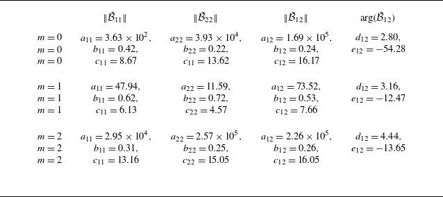
 B~2×2

 |m|⩽2
 St=0.1

 S^pp
 B~
 m⩽2
 M=0.4
 M=0.7
 M=0.8
 M=0.9
 S~pp
 B~
 Spp
 S~pp
 0.1⩽He⩽1

 S^pp
 m⩽2
 M=0.4
 M=0.7
 M=0.8
 M=0.9
 Spp
 a
 S^pp
 B~2×2
 m⩽2
 b
 S^pp
 B~2×2
 m⩽2
 S~pp
 0.1⩽He⩽1

 M=0.5
 S~pp
 B~
 m⩽2
 a
 b
 c
 d
 S~pp
 0.1⩽He⩽1
 Spp

 B5×5
 B~5×5
 B~
 B
 B
 B~
 B1,1
 B~1,1
 B2,2
 B~2,2
 B5,5
 B~5,5
 B1,2
 B~2,2

 S~pp
 B~
 m=0
 M=0.4
 Spp
 B
 B~
 B
 n=1
 n=2
 n=5
 0.1⩽He⩽1
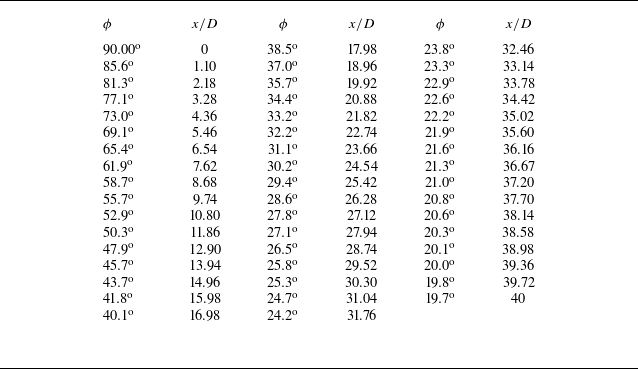

 m>0
 a
 d
 e
 h
 =0.3
 b
 d
 f
 h
 M=0.4
 M=0.7
 M=0.8
 M=0.9


