1 Introduction
Our concern is with exact coherent structures in shear flows. In particular, using a combination of asymptotic and numerical methods, we investigate how distributions of vortex–wave interaction states occur in quite arbitrary shear flows. The analysis will be based on a high number approximation, but we expect that the solutions extend to lower Reynolds numbers in much the same way as is the case in, for example, Couette flow. The analysis is partially motivated by recent experimental results on fully turbulent flows with the hope that the structures we describe might form the ‘backbone’ on which turbulent flows evolve in much the same manner as has been found to be the case for internal flows such as Couette flow or Hagen–Poiseuille flow; see, for example, Kawahara & Kida (Reference Kawahara and Kida2001).
Numerical investigations of nonlinear equilibrium states in shear flows began in the context of Couette flow with Nagata (Reference Nagata1990); more recently there have been numerous numerical descriptions of these states in channels and pipes by, for example, Wedin & Kerswell (Reference Wedin and Kerswell2004), Wang, Gibson & Waleffe (Reference Wang, Gibson and Waleffe2007) and Gibson, Halcrow & Cvitanovic (Reference Gibson, Halcrow and Cvitanovic2008). These solutions were christened as ‘self-sustained processes’, SSP for short by Waleffe (Reference Waleffe1997, Reference Waleffe2001), and were classified as lower or upper branch solutions by following them back to the saddle–node bifurcation from which they emanate. The lower branch solutions were subsequently found to play the role of edge states separating laminar and turbulent attractors – see, for example, Itano & Toh (Reference Itano and Toh2001) – whilst Kreilos & Eckhardt (Reference Kreilos and Eckhardt2012) showed that upper branch solutions undergo bifurcation cascades to new solutions which eventually lead to the formation of chaotic sets.
Some years before the SSP work mentioned above, Hall & Smith (Reference Hall and Smith1988, Reference Hall and Smith1991) had laid down a formal asymptotic fully nonlinear framework for what was described as vortex–wave interaction theory, VWI for short. The framework given was a quite general approach and can be applied to both inviscid (Rayleigh) and viscous (Tollmien–Schlichting) waves interacting with streamwise vortices. The theory was developed in order to describe the highly nonlinear processes involved in boundary layer transition, but it turned out that the relevance of the approach there was limited by the fact the receptivity process which internalises external mechanisms triggering disturbance growth in boundary layers did not predict a route to the VWI states. In recent years it has become common to refer to SSP or VWI states as exact coherent structures; the terminology is unfortunate as it leads to confusion with coherent structures loosely defined in the context of shear layer turbulence and acoustics.
The crucial feature of vortex–wave interaction theory is that it enables the Reynolds number to be scaled out of the problem and provides a rational closed interaction system describing the tripartite process allowing rolls, streaks and waves to coexist and support each other. In fact the process by which the wave interacts with itself to drive the roll through a stress jump across the wave’s critical layer is essentially the steady streaming mechanism associated with oscillatory flows; see, for example, Stuart (Reference Stuart1966). The only significant difference is that the layer where the Reynolds stresses associated with the oscillatory motion drive the process is bounded by fluid interfaces and so produces a stress jump rather than a velocity jump across its boundaries.
Some years later, motivated by the numerical results of Wang et al. (Reference Wang, Gibson and Waleffe2007), Hall & Sherwin (Reference Hall and Sherwin2010), hereafter HS1, applied the Hall & Smith (Reference Hall and Smith1991) formulation to plane Couette flow and showed that VWI theory was the formal high-Reynolds-number asymptotic description of lower branch SSP. Moreover, VWI theory was found to accurately predict the fully numerical calculations of SSP at remarkably low Reynolds numbers. Subsequently the upper branch of the curve in amplitude–wavenumber space describing the nonlinear states was given by Deguchi & Hall (Reference Deguchi and Hall2014) and thus VWI theory was shown to describe both upper and lower branch SSP states.
The work of HS1 was subsequently extended to a range of spanwise wavenumbers by Blackburn, Hall & Sherwin (Reference Blackburn, Hall and Sherwin2013), BHS for short, and it was shown that as the spanwise wavenumber
 $\unicode[STIX]{x1D6FD}$
increases, the VWI states for Couette flow deform into new canonical VWI states localised away from any boundaries. However, as was the case in HS1, only a lower branch state was found for a given streamwise wavenumber
 $\unicode[STIX]{x1D6FC}$
in a range
 $(0,\unicode[STIX]{x1D6FC}_{c}(\unicode[STIX]{x1D6FD}))$
and the question of whether there is an upper branch asymptotic state beyond the turning point
 $\unicode[STIX]{x1D6FC}=\unicode[STIX]{x1D6FC}_{c}$
remains unanswered.
At long streamwise wavelengths of the order of the Reynolds number, VWI theory fails and the states become long-wavelength structures satisfying the boundary-region equations; see Deguchi, Hall & Walton (Reference Deguchi, Hall and Walton2013). There it was found that as
 $\unicode[STIX]{x1D6FC}$
decreases the solutions develop a spatial localisation in the streamwise direction, with the flow having the tendency to vary on an
 $O(1)$
streamwise length scale excluded in the long-wavelength theory. Spanwise localised states have also been found in numerical investigations of channel flow equilibrium states; see Brand & Gibson (Reference Brand and Gibson2014). In pipe flows Willis & Kerswell (Reference Willis and Kerswell2009) have found states localised in the streamwise direction. In the channel flow case the localisation in the spanwise direction is akin to that known to occur in the Swift–Hohenberg equation often used to model Benard convection; see Thiele et al. (Reference Thiele, Archer, Robbins, Gomez and Knobloch2013). In the case of vortex–wave interactions involving Tollmien–Schlichting waves, localisation in the spanwise direction has been described by Dempsey et al. (Reference Dempsey, Deguchi, Hall and Walton2016).
It has in recent years become widely accepted that the SSP or VWI mechanism is implicated in the process by which near-wall streaks are generated in turbulent boundary layers; see, for example, Chernyshenko & Big (Reference Chernyshenko and Big2005). However, the work of Deguchi & Hall (Reference Deguchi and Hall2015) showed that near-wall streaks could be induced by nonlinear interactions at the edge of a boundary layer; this has clouded the issue somewhat. The streaks generated by the latter mechanism are smaller than those generated by VWI and so it is likely that VWI is the most relevant mechanism for near-wall streak generation. Further away from the wall in a turbulent boundary layer the mean part of the flow is thought to be described by von Kármán’s ‘law of the wall’; this has the velocity varying with the logarithm of the distance from the wall. This so-called ‘log layer’ is thicker than the near-wall region and therefore capable of supporting a wider range of roll–streak–wave wavelengths. The VWI mechanism essentially describes how a single downstream propagating wave interacts with itself to produce a spanwise periodic stress jump driving a roll flow which then interacts with the mean streamwise flow to produce a streak. Thus the existing VWI framework cannot be the mechanism enabling the log layer to persist because a single wave would just produce a stress jump at a single location normal to the wall. Here we investigate families of interacting VWI states involving waves of different wavespeeds and investigate whether such families can produce structures consistent with that in the log layer.
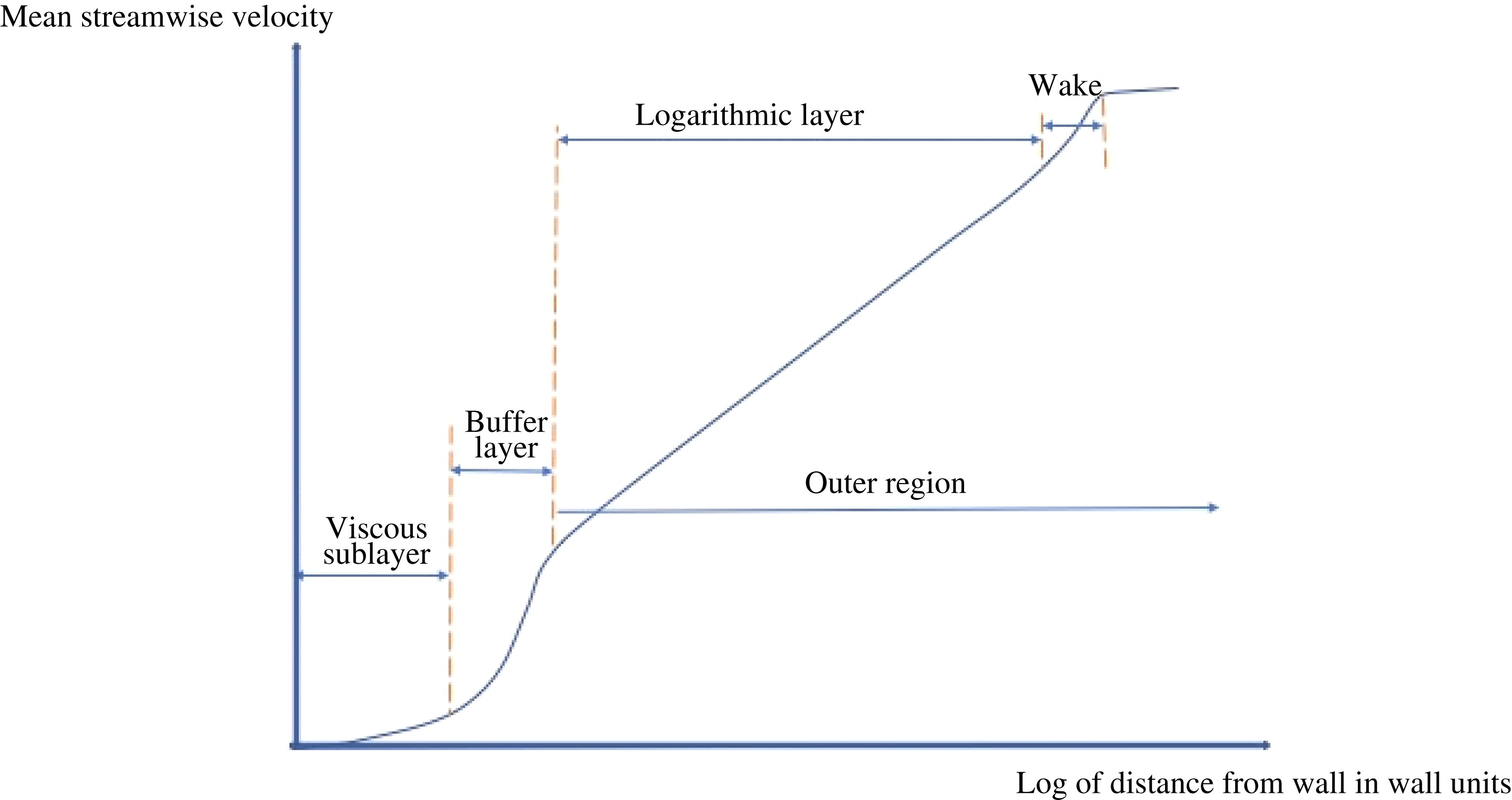
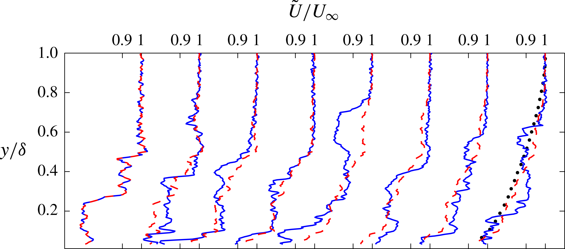
Figure 1 is a sketch of the mean velocity profile in a turbulent flow plotted against distance from the wall in wall units. Our interest is in VWI states which can occur in the log layer; indeed we will investigate whether the log layer could be driven by a distribution of VWI states. Figure 2 taken from Silva et al. (Reference Silva, Philip, Hutchins and Marusic2017) shows snapshots at different times of the instantaneous streamwise velocity (horizontal axis) at a given spanwise location as a function of
 $y/\unicode[STIX]{x1D6FF}$
, the distance from the wall, for
 $Re_{\unicode[STIX]{x1D70F}}=8000$
. Here
 $\unicode[STIX]{x1D6FF}$
is the boundary layer thickness. The blue lines are the instantaneous velocities, whilst each red dashed line is the cumulative average of the profiles taken from left to right. The black dotted curve is the converged mean streamwise velocity profile. We see that at any instant the profile seems to consist of regions of relatively constant momentum separated by shear layers. We will investigate whether such profiles are consistent with shear flows driven by families of VWI states separated by distances comparable to the distance between the shear layers.
The mean streamwise velocity (vertical axis) as a function of distance measured in wall units for a turbulent shear flow.

One reason why we expect a link between arrays of interacting VWI states in quite general shear flows and homogeneous turbulence can be explained as follows. Consider a flow predominantly in the
 $x$
direction which is homogeneous in the
 $x,z$
directions and suppose
 $U(y)$
is the mean (in
 $x,z$
) part of the streamwise velocity component. If the total velocity
 $\hat{\boldsymbol{U}}$
is written as
 $\hat{\boldsymbol{U}}=(U+u,v,w)$
then it is readily shown that
 $$\begin{eqnarray}0=-\frac{\text{d}(\overline{uv})}{\text{d}y}-\frac{\unicode[STIX]{x2202}P}{\unicode[STIX]{x2202}x}+\frac{1}{Re_{\unicode[STIX]{x1D70F}}}\frac{\unicode[STIX]{x2202}^{2}U}{\unicode[STIX]{x2202}y^{2}}.\end{eqnarray}$$
Here
 $\overline{uv}$
denotes the average of
 $uv$
in the
 $x{-}z$
plane,
 $Re_{\unicode[STIX]{x1D70F}}$
is the Reynolds number based on the friction velocity and
 $\unicode[STIX]{x2202}P/\unicode[STIX]{x2202}x$
is the streamwise pressure gradient. The equations for the fluctuating quantities
 $u,v,w$
can be written down by subtracting out
 $U$
, and they are of course nonlinear. The equations for the mean and the fluctuating quantities are coupled and, when used to model turbulence, some closure of the system is needed. If we think of a roll–streak–wave flow described by VWI theory as a mean streamwise flow, plus a fluctuating part made up of the roll, streak and wave flows, then the same kind of separation occurs. What VWI theory does is to provide a rational asymptotic way for closure of the two sets of equations rather than use a turbulence modelling approach where terms are retained or neglected based on arguments not necessarily backed by asymptotic analysis.
We shall see that VWI theory for distributed flows thus follows quite closely the spirit of turbulence closure models, but with the resulting equation for the mean
 $U$
a slightly modified form of the equation above. In fact the envelope equation associated with slowly varying distributions of vortex–wave interaction states is essentially the same as (1.1), the turbulent mean, except that the average term is simplified by the scale separations of VWI states and the small scales in the
 $y$
direction are also averaged out. We will see that for distributed slowly varying VWI states we have a situation similar to that found in turbulence models or in nonlinear small-wavelength Görtler vortices, see Hall & Lakin (Reference Hall and Lakin1988), where the mean state cannot be a priori specified and must be found from the interaction equations. A possible mechanism to support a single step of the staircase-like structure of figure 2 has been proposed recently by Chini et al. (Reference Chini, Montemuro, White and Klewicki2017). The mechanism is based on the VWI structure of Hall & Sherwin (Reference Hall and Sherwin2010) as applied to an isolated interaction. We comment further on this after describing the isolated interaction in the next section.
Instantaneous streamwise velocity in a turbulent shear flow as a function of distance from the wall. The horizontal axis denotes the streamwise velocity divided by its free stream value and the vertical axis denotes the distance from the wall scaled on boundary layer thickness. Figure is reproduced from Silva et al. (Reference Silva, Philip, Hutchins and Marusic2017).

Our first step described in §§ 2 and 3 will be to extend the original VWI structure of HS1 to allow for arrays of coupled interacting VWI states in a uniform infinite shear flow. The structures found are periodic in all three spatial directions and time. The process by which the states are sustained is identical to that discussed for Couette flow in HS1, but now there is an infinite set of waves of the same downstream wavenumber propagating downstream with wavespeeds differing by integer multiples of some reference speed. The key point is that to provide a stress jump capable of driving the roll field any wave can only successfully interact with itself and so, even though each wave is not periodic in the direction normal to its direction of propagation, the fact that there is a periodic array of waves identical apart from their wavespeed means that a triply periodic roll–streak–wave state can be sustained. The numerical method used to solve the interaction equations is given in § 4. Results of computations of the triply periodic VWI states are then given in § 5.
Having established this new form of exact coherent structure for a uniform shear flow we then investigate in § 6 how it can be embedded within an arbitrary shear flow. In § 7 we discuss the solution of the slow evolution equation similar to (1.1) which governs VWI arrays in arbitrary shear flows. In § 8 we will draw some conclusions.
2 Canonical localised exact coherent structures
VWI states localised in the wall normal direction were first found in BHS using the structure given in Hall & Sherwin (Reference Hall and Sherwin2010). Here we will quote the results from the two papers mentioned above. Consider the shear flow
 $$\begin{eqnarray}\boldsymbol{u}^{\ast }=(u^{\ast }(\boldsymbol{x}^{\ast }),v^{\ast }(\boldsymbol{x}^{\ast }),w^{\ast }(\boldsymbol{x}^{\ast })).\end{eqnarray}$$
In the above equations a
 $^{\ast }$
denotes a dimensional quantity and the flow is predominantly in the
 $x^{\ast }$
direction so we assume
 $v^{\ast },w^{\ast }$
are zero and that the dominant dependence of
 $u^{\ast }$
is on
 $y^{\ast }.$
The structure is taken to have typical wavelength
 $\hat{\unicode[STIX]{x1D706}}^{\ast }$
in the spanwise,
 $z^{\ast }$
, direction. We expand
 $u^{\ast }$
in the form
 $$\begin{eqnarray}u^{\ast }=u^{\ast }(\overline{y}^{\ast })+(y^{\ast }-\overline{y}^{\ast })u^{\ast \prime }(\overline{y}^{\ast })+\cdots =u^{\ast }(\overline{y}^{\ast })+\frac{(y^{\ast }-\overline{y}^{\ast })}{\hat{\unicode[STIX]{x1D706}}^{\ast }}\hat{\unicode[STIX]{x1D706}}^{\ast }u^{\ast \prime }(\overline{y}^{\ast })+\cdots \,,\end{eqnarray}$$
where a dash denotes a derivative with respect to
 $y^{\ast }$
. If we work in a frame moving downstream with speed
 $u^{\ast }(\overline{y}^{\ast })$
we can, without any loss of generality, set
 $u^{\ast }(\overline{y}^{\ast })=0$
. A typical flow velocity in a rectangular box of sides of length
 $O(\hat{\unicode[STIX]{x1D706}}^{\ast })$
centred on
 $y^{\ast }=\overline{y}^{\ast }$
is
 $\hat{\unicode[STIX]{x1D706}}^{\ast }u^{\ast \prime }(\overline{y}^{\ast })$
and so we define a Reynolds number associated with the flow in that box to be
 $$\begin{eqnarray}Re=\frac{(\hat{\unicode[STIX]{x1D706}}^{\ast })^{2}u^{\ast \prime }(\overline{y}^{\ast })}{\unicode[STIX]{x1D708}},\end{eqnarray}$$
where
 $\unicode[STIX]{x1D708}$
is the kinematic viscosity and write
 $$\begin{eqnarray}(x,y,z)=\frac{(x^{\ast },y^{\ast }-\overline{y}^{\ast },z^{\ast })}{\hat{\unicode[STIX]{x1D706}}^{\ast }},\quad t=t^{\ast }u^{\ast \prime }(\overline{y}^{\ast }).\end{eqnarray}$$
We scale the velocity and pressure fields in the form
 $$\begin{eqnarray}\boldsymbol{u}^{\ast }=\hat{\unicode[STIX]{x1D706}}^{\ast }u^{\ast \prime }(\overline{y}^{\ast })\widehat{\boldsymbol{U}}(x,t),\quad p^{\ast }=\unicode[STIX]{x1D70C}^{\ast }(\hat{\unicode[STIX]{x1D706}}u^{\ast \prime }(\overline{y}^{\ast }))^{2}\widehat{p}.\end{eqnarray}$$
The equations of motion for the fluid in the box become
 $$\begin{eqnarray}\displaystyle & \displaystyle \frac{\text{D}\widehat{\boldsymbol{U}}}{\text{D}t}=-\unicode[STIX]{x1D735}\widehat{p}+\frac{1}{Re}\unicode[STIX]{x1D6FB}^{2}\widehat{\boldsymbol{U}}, & \displaystyle\end{eqnarray}$$
 $$\begin{eqnarray}\displaystyle & \displaystyle \unicode[STIX]{x1D735}\boldsymbol{\cdot }\widehat{\boldsymbol{U}}=0. & \displaystyle\end{eqnarray}$$
Solutions of these equations localised in the
 $y$
direction constitute the class of VWI solutions we refer to as the canonical localised VWI states. For completeness we shall now write down the essential details of the formal expansion procedure to describe VWI interactions; we shall do this in the context of the Navier–Stokes equations in the form shown in (2.6)–(2.7). Following HS1 we consider the roll–streak–wave flow
 $$\begin{eqnarray}\displaystyle & \displaystyle \widehat{\boldsymbol{U}}(y,z)=\left(y+U,\frac{V}{Re},\frac{W}{Re}\right)+\unicode[STIX]{x1D70C}\left[\frac{\text{e}^{\text{i}\unicode[STIX]{x1D6FC}(x-ct)}}{Re^{7/6}}(u(y,z),v(y,z),w(y,z))+\text{c.c.}\right]+\cdots \qquad & \displaystyle\end{eqnarray}$$
 $$\begin{eqnarray}\displaystyle & \displaystyle \widehat{P}=\frac{P(y,z)}{Re}+\unicode[STIX]{x1D70C}\left[\frac{\text{e}^{\text{i}\unicode[STIX]{x1D6FC}(x-ct)}}{Re^{7/6}}p(y,z)+\text{c.c.}\right]+\cdots \,. & \displaystyle\end{eqnarray}$$
We refer to
 $U$
as the streak and
 $y+U$
as the total streak flow. What we refer to as the ‘roll’ corresponds to the flow associated with
 $V/Re,W/Re$
in (2.8). The size of the wave term of scaled amplitude
 $\unicode[STIX]{x1D70C}$
is fixed as in Hall & Smith (Reference Hall and Smith1991), HS2 for short, such that the Reynolds stresses associated with the wave in the critical layer where
 $y+U=c$
produce an
 $O(1)$
jump in the roll stresses across the critical layer. Substituting the above expansions into (2.6)–(2.7) we find that the roll and streak problems decouple and take the form
 $$\begin{eqnarray}\displaystyle & V+VU_{y}+WU_{z}=U_{yy}+U_{zz}, & \displaystyle\end{eqnarray}$$
 $$\begin{eqnarray}\displaystyle & VV_{y}+WV_{z}=-P_{y}+V_{yy}+V_{zz}, & \displaystyle\end{eqnarray}$$
 $$\begin{eqnarray}\displaystyle & VW_{y}+WW_{z}=-P_{z}+W_{yy}+W_{zz}, & \displaystyle\end{eqnarray}$$
 $$\begin{eqnarray}\displaystyle & V_{y}+W_{z}=0. & \displaystyle\end{eqnarray}$$
We are interested in spanwise periodic flows and so the roll–streak equations must be solved subject to
 $\boldsymbol{U}$
,
 $P$
being periodic in
 $z$
with wavelength unity. We are interested in the canonical states localised in
 $y$
and so, as noted in BHS, the roll–streak equations must be solved subject to
 $U_{y},V,W$
all vanishing at
 $\pm \infty$
.
The wavenumber
 $\unicode[STIX]{x1D6FC}$
and the wavespeed
 $c$
are assumed real so that the wave is always neutral and, following the analysis of Hall & Horseman (Reference Hall and Horseman1991), we see that the wave satisfies the equation
 $$\begin{eqnarray}\left[\frac{p_{y}}{F^{2}}\right]_{y}+\left[\frac{p_{z}}{F^{2}}\right]_{z}-\frac{\unicode[STIX]{x1D6FC}^{2}p}{F^{2}}=0,\end{eqnarray}$$
where
 $F=y+U-c$
. This equation becomes singular on the curve
 $y=f(z)$
, where
 $F=0$
and a viscous critical layer is required to regularise the disturbance field.
The roll–streak system and the wave pressure equation must be solved subject to periodicity in
 $z$
and the vanishing of the roll–streak flow at large distances from
 $y=0$
. Thus we must solve (2.10)–(2.14) subject to
 $$\begin{eqnarray}U_{y},V,W,p\rightarrow 0,\quad y\rightarrow \pm \infty ,\end{eqnarray}$$
and
 $$\begin{eqnarray}\boldsymbol{U}(y,z+2\unicode[STIX]{x03C0})=\boldsymbol{U}(y,z),p(y,z+2\unicode[STIX]{x03C0})=p(y,z).\end{eqnarray}$$
Note here that the conditions on
 $U$
at
 $\pm \infty$
allow for a finite jump in
 $U$
across the layer; see Deguchi & Hall (Reference Deguchi and Hall2014) for how that jump is accommodated by the outer unperturbed flow. The system is closed by solving for the flow in the critical layer straddling
 $y=f$
; the upshot is that when crossing the critical layer the roll stresses undergo the jumps:
 $$\begin{eqnarray}\displaystyle & \displaystyle \left[\frac{\unicode[STIX]{x2202}{\mathcal{V}}^{s}(n,s)}{\unicode[STIX]{x2202}n}\right]_{-}^{+}=n_{0}\unicode[STIX]{x1D70C}^{2}\unicode[STIX]{x1D6FC}^{-5/3}\frac{\unicode[STIX]{x2202}}{\unicode[STIX]{x2202}s}\left(\hat{\unicode[STIX]{x1D706}}_{1}^{-5/3}\left|\frac{\unicode[STIX]{x2202}Q}{\unicode[STIX]{x2202}s}\right|^{2}\right), & \displaystyle\end{eqnarray}$$
 $$\begin{eqnarray}\displaystyle & \displaystyle [P]_{-}^{+}=-n_{0}\unicode[STIX]{x1D70C}^{2}\unicode[STIX]{x1D6FC}^{-5/3}\hat{\unicode[STIX]{x1D706}}_{1}u^{-5/3}\hat{\unicode[STIX]{x1D706}}_{0}\left|\frac{\unicode[STIX]{x2202}Q}{\unicode[STIX]{x2202}s}\right|^{2}, & \displaystyle\end{eqnarray}$$
where
 $n_{0}=2\unicode[STIX]{x03C0}(2/3)^{2/3}$
and
 $n,s$
are body-fitted coordinates normal and along the critical layer,
 $\hat{\unicode[STIX]{x1D706}}_{1}=\unicode[STIX]{x2202}/\unicode[STIX]{x2202}n[y+U]$
at
 $y=f,\hat{\unicode[STIX]{x1D706}}_{0}$
is the local curvature of the critical layer,
 ${\mathcal{V}}^{s}$
is
 $(V,W)$
resolved along the tangent to the critical layer, and
 $Q(s)$
is the wave pressure
 $p$
evaluated on the critical layer. The roll, streak and wave equations (2.10)–(2.18), together with a normalisation condition on the wave pressure, constitute the VWI description of exact coherent structures and define a nonlinear eigenvalue problem for the wavespeed
 $c$
and amplitude
 $\unicode[STIX]{x1D70C}$
in terms of the streamwise wavenumber
 $\unicode[STIX]{x1D6FC}$
. For mirror-symmetric modes, which will be our concern here, there is a significant simplification in that the critical layer becomes flat, in which case there is no jump in
 $P$
across the critical layer, which is now at
 $y=0$
. The structure proposed by Chini et al. (Reference Chini, Montemuro, White and Klewicki2017) is a variant of (2.10)–(2.18). The structure proposed would require the VWI interaction equations for a localised interaction to be embedded in a mean flow tending to constants at
 $\pm \infty$
; it is not clear that such a constraint can be applied over an infinite interval.
We define
 $U^{L},V^{L},W^{L},P^{L},p^{L}$
to be a solution of (2.10)–(2.18) with
 $c=0$
and mirror symmetry about
 $y=0$
. For future reference we also note that these quantities are functions of
 $y,z$
and, along with the wave amplitude
 $\unicode[STIX]{x1D70C}$
, also depend on the streamwise wavenumber
 $\unicode[STIX]{x1D6FC}$
. Thus they represent a one-parameter family of solutions of the VWI equations for localised mirror-symmetric states, and we can write, for example,
 $U^{L}=U^{L}(\unicode[STIX]{x1D6FC},y,z)$
.
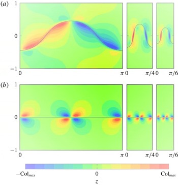
Contours of constant streamwise vorticity for the sinuous (a) and mirror-symmetric (b) modes in Couette flow for
 $\unicode[STIX]{x1D6FC}/\unicode[STIX]{x1D6FD}=0.5$
and
 $\unicode[STIX]{x1D6FD}=2,4,12$
from left to right. The results correspond to full Navier–Stokes solutions at
 $Re=30\,000$
. The black line represents the location of the critical layer.

Figure 3 gives results from the full Navier–Stokes equations showing how the localised sinuous and mirror-symmetric modes develop from Couette flow states. The results are for
 $Re=30\,000$
with the streamwise and spanwise wavenumbers fixed and in the ratio 1 : 2. The results show contours of constant streamwise vorticity in the
 $y{-}z$
plane for sinuous and mirror-symmetric modes in (a,c), respectively. In each panel the results shown from left to right correspond to
 $\unicode[STIX]{x1D6FD}=2,8,12$
.
Now let us comment on the possible relevance of localised canonical VWI states to the law of the wall. We suppose that there is a distribution of VWI states of the form discussed above, separated by a distance
 $d$
which is large compared to the VWI-wavelength scale
 $\hat{\unicode[STIX]{x1D706}}^{\ast }$
. The separation of the states means there is no interaction between them and they will together lead to an order
 $\hat{\unicode[STIX]{x1D706}}^{\ast }/d$
correction to the mean flow
 $u^{\ast }$
.
The usual derivations of the law of the wall insist on self-similarity of the flow in the log layer based on the assertion that there is no length scale in the problem. In the situation envisaged above that requires that the family of VWI states introduced in the flow must be identical when they are written in terms of their distance from the wall. From the definition of
 $x,y,z$
in (2.4) it therefore follows that, if self-similarity is present, the localised structures can only correspond to the same VWI state, subject to magnification, if
 $\hat{\unicode[STIX]{x1D706}}^{\ast }\sim \overline{y}^{\ast }$
. For self-similarity of the velocity field the form of (2.5) then requires that
 $\hat{\unicode[STIX]{x1D706}}^{\ast }u^{\ast \prime }(\overline{y}^{\ast })$
is independent of
 $\overline{y}^{\ast }$
. It follows that
 $$\begin{eqnarray}u^{\ast \prime }(y^{\ast })=\frac{H}{y^{\ast }},\end{eqnarray}$$
where
 $H$
is a constant. It follows that
 $$\begin{eqnarray}u^{\ast }(y^{\ast })=H\ln y^{\ast }+J,\end{eqnarray}$$
where
 $J$
is a constant. This is of course von Kármán’s law of the wall. Thus we see that if a distribution of self-similar VWI interactions exists then the mean flow satisfies the law of the wall. In other words a logarithmic profile is the only flow which allows for a family of self-similar states, but it is not self-sustaining. That it cannot be self-sustaining follows from the first condition in (2.14), which means that the states together produce at most an order
 $\hat{\unicode[STIX]{x1D706}}^{\ast }/d$
correction to the mean state. Hence the jump produced by a family of interactions cannot drive the leading-order mean flow
 $u^{\ast }$
. The conclusion then is that, though the condition for the existence of a distribution of non-interacting identical VWI states requires the mean flow to satisfy the law of the wall, there is no mechanism present to sustain the logarithmic profile. The obvious modification is therefore to bring the VWI states sufficiently close together.
The simplest case to consider is when the VWI states are brought together to form a periodic array in the
 $y$
direction. We will begin by considering such a possibility within an infinite uniform shear flow, and later extend that to quite arbitrary shear flows. Even for the case of an infinite uniform shear flow there are many ways in which identical localised VWI states can be brought together. Here we will consider perhaps the simplest case, where an infinite set of mirror-symmetric states of the type shown in figure 3(c) are brought together with no phase difference introduced in the
 $z$
direction.
3 Canonical periodic exact coherent structures
In order to set the scene for the new family of more general canonical VWI states it is useful to recap on the key features of the basic VWI. Firstly, the wave part of the state exists as a neutrally stable linear inviscid instability of the streak. Away from the critical layer the self-interaction of the wave is weak and it does not reinforce the roll flow. However, in the critical layer where the wave moves with the same speed as the flow in the streamwise direction the equation for the wave becomes singular and the wave velocity grows inversely with distance from the critical layer. That growth is checked by viscous effects and the critical layer does not become sufficiently large for it to be nonlinear as in, for example, Benney & Bergeron (Reference Benney and Bergeron1966). The growth of the wave in the critical layer causes the self-interaction of the wave to intensify and at quadratic order produces an
 $O(1)$
jump in the roll stresses across the layer.
It is clear that VWI states can exist with multiple waves with different critical layers so long as each exists as a neutral wave of the streak. The interaction of the different waves does not contribute to the roll stress jumps because each wave only blows up within its own critical layer. But it would be unusual for a given streak to support a number of neutral waves, and so not surprisingly such states have not yet been identified. Nevertheless we could, however, imagine a situation where individual localised VWI states are brought together sufficiently close for some interaction to occur; the states we now describe can be viewed as a result of such a procedure.
Our starting point is once again (2.6)–(2.7), but we now assume that in the unperturbed case the basic flow is the uniform shear flow
 $\hat{\boldsymbol{U}}=(y,0,0)$
. How the structures we now derive for the latter case fit into a more general shear flow will be addressed later. The first step is to assume that the roll–streak flow
 $(U,V,W)$
flow is now periodic in both
 $y$
and
 $z$
. In the description given above for localised VWI states the spanwise wavelength was used as the length scale for the interaction. In order to more easily account for more general flows later in this paper it is convenient to now chose the wavelength of the array of VWI states in the
 $y$
direction as the appropriate length scale.
It is important to note that the total streak
 $y+U$
itself is not periodic in
 $y$
, it is the difference between the total streak and the unperturbed linear shear profile that is periodic in
 $y$
. That is important because the pressure wave equation for each individual wave depends on the total streak, and therefore is not to be solved subject to periodicity in
 $y$
. The wavelengths in the
 $y,z$
directions are comparable, so the change in scaling is taken care of by allowing the VWI state to be periodic in
 $z$
with wavenumber
 $\unicode[STIX]{x1D6FD}$
. For convenience we will define
 $Z=\unicode[STIX]{x1D6FD}z$
, and therefore seek solutions in
 $Z$
with period
 $2\unicode[STIX]{x03C0}$
. Now consider a zero-frequency inviscid wave disturbance to the streak flow
 $y+U(y,Z)$
. If the wave is once again proportional to
 $\text{e}^{\text{i}\unicode[STIX]{x1D6FC}(x-ct)}$
then the wave pressure will satisfy (2.14), but with the latter written in terms of
 $Z$
rather than
 $z$
. Suppose that the equation is again solved subject to
 $p$
vanishing at
 $\pm \infty$
.
Now consider the wave with
 $c$
replaced by
 $c+n$
, where
 $n$
is any integer. Since the total streak
 $y+U$
has
 $U$
periodic in
 $y$
with period unity, it follows by shifting the origin to
 $y=n$
that the wave pressure of this disturbance is the wave pressure of the
 $c=0$
wave, but with
 $y$
replaced by
 $y-n$
. Thus, if we superimpose on the streak an infinite set of waves of the same streamwise wavenumber but with wave speeds differing by unity we can express the ‘
 $n$
th’ wave field in terms of that of the
 $c=0$
wave. Within the VWI framework we know that it is the interaction of a wave with itself in its critical layer which drives the roll enabling the roll field to exist. Now when we have an infinite number of waves we simply consider the interaction of each distinct wave with itself, the cross-interactions are a higher-order effect since the critical layers for the waves are distinct. In other words we can treat the waves as if they exist in isolation from each other and the only difference between them is the location of the different critical layers. Since we have assumed the wavespeeds differ by unity it follows that the self-interactions of each of the infinite set of waves will generate a periodic (in
 $y$
) set of roll stress jumps across the periodically spaced critical layers. This is the self-sustaining mechanism for the new type of periodic array of exact coherent structures. We now write down the formal asymptotic expansion defining the process just outlined. We modify (2.8)–(2.9) by writing
 $$\begin{eqnarray}\displaystyle & \displaystyle \widehat{U}=y+U(y,Z)+\frac{\text{e}^{\text{i}\unicode[STIX]{x1D6FC}X}}{Re^{7/6}}\mathop{\sum }_{-\infty }^{\infty }\unicode[STIX]{x1D70C}\text{e}^{-\text{i}n\unicode[STIX]{x1D6FC}t}u(y-n,Z)+\text{c.c.}\cdots \,, & \displaystyle\end{eqnarray}$$
 $$\begin{eqnarray}\displaystyle & \displaystyle \widehat{V}=\frac{V(y,Z)}{Re}+\frac{\text{e}^{\text{i}\unicode[STIX]{x1D6FC}X}}{Re^{7/6}}\mathop{\sum }_{-\infty }^{\infty }\unicode[STIX]{x1D70C}\text{e}^{-\text{i}n\unicode[STIX]{x1D6FC}t}v(y-n,Z)+\text{c.c.}\cdots \,, & \displaystyle\end{eqnarray}$$
 $$\begin{eqnarray}\displaystyle & \displaystyle \widehat{W}=\frac{W(y,Z)}{Re}+\frac{\text{e}^{\text{i}\unicode[STIX]{x1D6FC}X}}{Re^{7/6}}\mathop{\sum }_{-\infty }^{\infty }\unicode[STIX]{x1D70C}\text{e}^{-\text{i}n\unicode[STIX]{x1D6FC}t}w(y-n,Z)+\text{c.c.}\cdots \,, & \displaystyle\end{eqnarray}$$
 $$\begin{eqnarray}\displaystyle & \displaystyle \widehat{P}=\frac{P(y,Z)}{Re}+\frac{\text{e}^{\text{i}\unicode[STIX]{x1D6FC}X}}{Re^{7/6}}\mathop{\sum }_{-\infty }^{\infty }\unicode[STIX]{x1D70C}\text{e}^{-\text{i}n\unicode[STIX]{x1D6FC}t}p(y-n,Z)+\text{c.c.}\cdots \,. & \displaystyle\end{eqnarray}$$
Thus we have replaced the single wave in the localised VWI problem by an infinite sum of waves of the same amplitude and wavenumber but with wavespeeds differing by unity. That means that ‘
 $n$
th’ wave has its critical layer at
 $y=n$
, where it interacts with itself to produce a jump in the roll shear. We know from (2.17) to (2.18) that the stress jumps depend on the modulus of the wave pressure along its critical layer, so, without changing the overall interaction equations, we could generalise the above expansion to allow for arbitrary phase differences between the waves. The periodicity of the roll–streak flow is therefore supported by a periodic array of waves, each of which interacts significantly only with itself to produce the required local shear stress jump across its own critical layer. The roll–streak equations become
 $$\begin{eqnarray}\displaystyle & V+VUy+\unicode[STIX]{x1D6FD}WU_{Z}=U_{yy}+\unicode[STIX]{x1D6FD}^{2}U_{ZZ}, & \displaystyle\end{eqnarray}$$
 $$\begin{eqnarray}\displaystyle & VV_{y}+\unicode[STIX]{x1D6FD}WV_{Z}=-P_{y}+V_{yy}+\unicode[STIX]{x1D6FD}^{2}V_{ZZ}, & \displaystyle\end{eqnarray}$$
 $$\begin{eqnarray}\displaystyle & VW_{y}+\unicode[STIX]{x1D6FD}WW_{Z}=-\unicode[STIX]{x1D6FD}P_{z}+W_{yy}+\unicode[STIX]{x1D6FD}^{2}W_{ZZ}, & \displaystyle\end{eqnarray}$$
 $$\begin{eqnarray}\displaystyle & V_{y}+\unicode[STIX]{x1D6FD}W_{Z}=0. & \displaystyle\end{eqnarray}$$
Note that we choose to work with variable
 $Z$
rather than
 $z$
in order to facilitate comparison with the more general case to be discussed later. The wave pressure function
 $p$
satisfies
 $$\begin{eqnarray}\left(\frac{p_{y}}{[y+U(y,Z)]^{2}}\right)_{y}+\unicode[STIX]{x1D6FD}^{2}\left(\frac{p_{Z}}{[y+U(y,Z)]^{2}}\right)_{Z}-\frac{\unicode[STIX]{x1D6FC}^{2}p}{[y+U(y,Z)]^{2}}=0,\end{eqnarray}$$
Note, however, that the wave pressure function is not periodic in
 $y$
and so the above equation is to be solved subject to
 $$\begin{eqnarray}\displaystyle p\rightarrow 0,\quad y\rightarrow \pm \infty . & & \displaystyle\end{eqnarray}$$
The conditions to be imposed on the roll–streak flow are periodicity in
 $y,Z$
so that
 $$\begin{eqnarray}\displaystyle & \boldsymbol{U}(y+1,Z)=\boldsymbol{U}(y,Z+2\unicode[STIX]{x03C0})=\boldsymbol{U}(y,Z), & \displaystyle\end{eqnarray}$$
 $$\begin{eqnarray}\displaystyle & P(y+1)=P(y,Z+2\unicode[STIX]{x03C0})=P(y,Z). & \displaystyle\end{eqnarray}$$
We restrict attention to mirror-symmetric states so the jump conditions arising from the interaction of each wave with itself leads to the jump conditions
 $$\begin{eqnarray}\displaystyle & \displaystyle \left[\frac{\unicode[STIX]{x2202}W}{\unicode[STIX]{x2202}y}\right]_{-}^{+}=n_{0}\unicode[STIX]{x1D70C}^{2}\unicode[STIX]{x1D6FD}^{3}\unicode[STIX]{x1D6FC}^{-5/3}\frac{\unicode[STIX]{x2202}}{\unicode[STIX]{x2202}Z}\left(\hat{\unicode[STIX]{x1D706}}^{-5/3}\left|\frac{\unicode[STIX]{x2202}Q}{\unicode[STIX]{x2202}Z}\right|^{2}\right), & \displaystyle\end{eqnarray}$$
 $$\begin{eqnarray}\displaystyle & \displaystyle [P]_{-}^{+}=0, & \displaystyle\end{eqnarray}$$
across each critical layer. In the above equation
 $\hat{\unicode[STIX]{x1D706}}(z)=1+U_{y}(0,Z)$
is the local shear at the critical layer and
 $Q$
is the wave pressure evaluated along the critical layer
 $y=0$
. Finally, the wave pressure function
 $p$
has been normalised such that
 $$\begin{eqnarray}\int _{-\infty }^{\infty }p(0,Z)p^{\ast }(0,Z)\,\text{d}Z=1.\end{eqnarray}$$
The equations (3.5)–(3.15) define the nonlinear eigenvalue for an infinite periodic array of mirror-symmetric exact coherent structures. Given the above normalisation the eigenvalue problem determines the wave amplitude
 $\unicode[STIX]{x1D70C}$
as a function of
 $\unicode[STIX]{x1D6FC},\unicode[STIX]{x1D6FD}$
. For ease of comparison with the non-local theory which follows later we denote the roll–streak flow of an equilibrium exact periodic coherent structure by
 $\boldsymbol{{\mathcal{U}}}(\unicode[STIX]{x1D6FC},\unicode[STIX]{x1D6FD},y,Z),{\mathcal{P}}(\unicode[STIX]{x1D6FC},\unicode[STIX]{x1D6FD},y,Z)$
. The eigenrelation for the wave amplitude can be written in the form
 $$\begin{eqnarray}\unicode[STIX]{x1D70C}={\mathcal{F}}(\unicode[STIX]{x1D6FC},\unicode[STIX]{x1D6FD}).\end{eqnarray}$$
The equations describing the new kind of periodically distributed exact coherent structures describe all possible VWI states whatever their symmetry properties. For definiteness we shall here concentrate on the so-called mirror-symmetric structures; these are easier to deal with than sinuous structures since they have flat critical layers and so the associated computations do not have to be quite so sophisticated. The mirror-symmetric structure we investigate has the property that the wave part of the flow has twice the spanwise wavelength of the roll–streak flow. For a discussion of such structures in Couette flow see Maestri (Reference Maestri2015); interestingly it was found in the latter case that there was also a mirror-symmetric state possible with the pressure wave having spanwise wavelength four times that of the roll–streak flow.
4 Numerical solution of the VWI equations for periodic arrays
The essential difficulty associated with the solution of the interaction equations is the implementation of the jump conditions across the critical layer. In Hall & Sherwin (Reference Hall and Sherwin2010) the problem was taken care of by introducing forcing terms in the roll equations which automatically produced the correct jumps; however, doing so introduced a parameter representing the thickness of the regularising delta function layer. In addition, viscosity was introduced into the wave pressure eigenvalue problem to avoid its singular nature at the critical layer. Thus solutions of the VWI problem were then obtained by taking the appropriate limits of those regularisation parameters. In BHS the same difficulties were resolved by retaining the viscous terms in the wave pressure problem and the quadratic terms involving the wave were left in the roll equations to induce the required stress jumps rather than applying the jump conditions directly. The latter approach is easier in the sense that it involves only one physical parameter, the Reynolds number. We first consider the form of the wave pressure as the critical layer is approached. If we work in ‘body-fitted’ coordinates
 $(n,s)$
normal and along the critical layer, and expand the streak
 $y+U(y,z)$
near the critical layer as
 $$\begin{eqnarray}y+U=\unicode[STIX]{x1D707}_{1}(s)n+\unicode[STIX]{x1D707}_{2}(s)n^{2}+\cdots\end{eqnarray}$$
we find that
 $u,v,w\backsim 1/(y-f)$
as the critical layer is approached and at the critical layer the three velocity components of the leading order wavefield are therefore of size
 $R^{-5/6}$
since the critical layer is viscous and of thickness
 $R^{-1/3}$
. In order to find the form of the wave within the critical layer we need to determine the series form of the pressure as the layer is approached. This is most easily achieved by writing the wave pressure equation in terms of the coordinates
 $(n,s)$
normal and along the critical layer, we find that (3.9) becomes
 $$\begin{eqnarray}\frac{\unicode[STIX]{x2202}^{2}p}{\unicode[STIX]{x2202}n^{2}}+\left[\frac{\unicode[STIX]{x1D712}}{{\mathcal{G}}}-\frac{2{\displaystyle \frac{\unicode[STIX]{x2202}[y+U]}{\unicode[STIX]{x2202}n}}}{y+U-c}\right]\frac{\unicode[STIX]{x2202}p}{\unicode[STIX]{x2202}n}+\frac{1}{{\mathcal{G}}^{2}}\frac{\unicode[STIX]{x2202}^{2}p}{\unicode[STIX]{x2202}s^{2}}-\left[\frac{\unicode[STIX]{x1D712}^{\prime }n}{{\mathcal{G}}^{3}}+\frac{2{\displaystyle \frac{\unicode[STIX]{x2202}u}{\unicode[STIX]{x2202}s}}}{[y+U-c]{\mathcal{G}}^{2}}\right]\frac{\unicode[STIX]{x2202}p}{\unicode[STIX]{x2202}s}-\unicode[STIX]{x1D6FC}^{2}p=0,\end{eqnarray}$$
where
 $\unicode[STIX]{x1D712}$
is the curvature of the critical layer and
 ${\mathcal{G}}=1+\unicode[STIX]{x1D712}n$
. The Frobenius solution of the wave pressure equation for small
 $n$
takes the form
 $$\begin{eqnarray}\displaystyle p=p_{0}(s)+p_{2}(s)n^{2}+p_{3L}(s)n^{3}\ln n+p_{3}(s)n^{3}+\cdots \,. & & \displaystyle\end{eqnarray}$$
Here
 $p_{0},p_{2}\ldots \ldots$
are functions of
 $s$
, and
 $$\begin{eqnarray}p_{2}=\frac{1}{2}\left[\left(\frac{p_{0s}}{\unicode[STIX]{x1D707}_{1}^{2}}\right)_{s}-\unicode[STIX]{x1D6FC}^{2}p_{0}\right]^{\prime }\end{eqnarray}$$
and
 $$\begin{eqnarray}p_{3L}=\frac{p_{2}}{3}\left[\frac{4\unicode[STIX]{x1D707}_{2}}{\unicode[STIX]{x1D707}_{1}}-2\unicode[STIX]{x1D712}\right]+\frac{2}{3}\unicode[STIX]{x1D712}p_{0ss}-\frac{2}{3}\frac{\unicode[STIX]{x1D707}_{1}^{\prime }}{\unicode[STIX]{x1D707}_{1}}\left[2\unicode[STIX]{x1D712}+\frac{\unicode[STIX]{x1D707}_{2}^{\prime }}{\unicode[STIX]{x1D707}_{1}^{\prime }}+\frac{\unicode[STIX]{x1D707}_{2}}{\unicode[STIX]{x1D707}_{1}}\right].\end{eqnarray}$$
Thus the singular nature of the wave pressure equation manifests itself through the generation of the
 $n^{3}\ln n$
term above. However, we see that the singular term vanishes if the critical layer is flat and
 $\unicode[STIX]{x1D707}_{2}=0$
. This situation is equivalent to the situation for the classical Rayleigh equation when an inflection point exists. In this paper we henceforth restrict our attention to the case when
 $U$
and hence
 $y+U$
are odd functions of
 $y$
. This simplifies the problem significantly since the critical layers associated with the waves are all flat and the jump conditions reduce to a simpler form, indeed there is now no jump for the roll pressure. Moreover, the numerical computation of the wave from the wave pressure equation turns out to be relatively easy since the critical layer associated with each wave turns out to be a regular singular point. Note, however, that even though the wave pressure is no longer singular the
 $x,Z$
components of the wave velocity still blow up inversely with distance from the critical layer, and so a viscous critical layer is still needed.
We now describe how we solved the wave pressure equation (3.9) with
 $U$
now corresponding to the distributed periodic case. If the streak field is known we can discretise (3.9) using finite differences in both
 $x$
and
 $Z$
using the scheme given by Hall & Horseman (Reference Hall and Horseman1991); the reader is referred to that paper for details of the process. In that paper the complex wavespeed was calculated as a function of the real wavespeed
 $\unicode[STIX]{x1D6FC}$
for a given value of
 $\unicode[STIX]{x1D6FD}$
, the spanwise wavenumber. Here our interest is in eigenvalues with
 $c=0$
and so, for a given streak field, we iterate to find the corresponding real eigenvalue
 $\unicode[STIX]{x1D6FC}$
. The grid used has step lengths
 $h_{y}$
and
 $h_{Z}$
in the
 $y,Z$
directions, respectively. The modes of interest here have the wave a 1 : 2 subharmonic of the roll–streak field in the spanwise direction. If the streak is even in
 $Z$
we can therefore choose to look for wave pressure fields which have
 $p_{Z}=0$
at
 $Z=0$
and
 $p=0$
at
 $Z=\unicode[STIX]{x03C0}/2$
; therefore, we need only solve the wave pressure equation on
 $0\leqslant z\leqslant \unicode[STIX]{x03C0}/2$
. In the
 $y$
direction we look for solutions even in
 $y$
and so need only consider
 $0\leqslant y\leqslant \infty$
. In view of the singular nature of the wave pressure equation at
 $y=0$
we take the first grid point in the
 $y$
direction to be at
 $y=h_{y}$
. The wave pressure field at
 $y=0$
will appear in the discretised equations, but is replaced by a combination of the pressure at
 $h_{y},2h_{y},3h_{y}$
after; noting that the pressure is even in
 $y$
, we can set
 $p_{yyy}=0$
at
 $y=0$
. Having found an eigenvalue and eigenfunction of the wave pressure equation for the given streak field, the jump conditions can then be computed.
The roll–streak equations were solved using the spectral/finite difference procedure given in Hall (Reference Hall1988) in the context of nonlinear spatially growing Görtler vortices. In view of the periodicity in
 $y$
we need only solve the equations on
 $(0,1)$
. The jump conditions now have zero jump in
 $P$
and thus only a jump in
 $W_{y}$
at
 $y=0,1$
. The required solution has
 $U,V$
even in
 $Z$
and
 $W$
odd in
 $Z$
. In the vertical direction we seek solutions which, with respect to
 $y=1/2$
, have
 $W$
even in
 $y$
with
 $U,V$
odd in
 $y.$
That symmetry enables us to solve the equations only on
 $(0,1/2)$
, so that in
 $y$
we impose the conditions
 $$\begin{eqnarray}U=V=0,\quad W_{y}=\frac{1}{2}n_{0}\unicode[STIX]{x1D6FD}^{3}\unicode[STIX]{x1D70C}^{2}\unicode[STIX]{x1D6FC}^{-5/3}\frac{\unicode[STIX]{x2202}}{\unicode[STIX]{x2202}Z}(\hat{\unicode[STIX]{x1D706}}^{-5/3}{Q_{Z}}^{2}),\quad y=0,\end{eqnarray}$$
and
 $$\begin{eqnarray}U=V=W_{y}=0,\quad y={\textstyle \frac{1}{2}}.\end{eqnarray}$$
Note above that for the mirror-symmetric modes we can take the wave pressure
 $Q=p_{0}(Z)$
on the critical layer to be real.
Next we reintroduce the time derivatives into the roll–streak equations and, for a given set of jump conditions, use the procedure of Hall (Reference Hall1988) to march them forward in time until they reach steady state. Thus, following Hall (Reference Hall1988) we obtained a solution by expanding
 $U,V$
in a Fourier cosine series in
 $z$
together with a Fourier sine series expansion for
 $W$
. In the vertical direction we used a finite difference approach, once again following Hall (Reference Hall1988). Thus, for example, when we present results,
 $U_{0}$
represents the zeroth Fourier cosine coefficient in the expansion of
 $U$
whilst
 $V_{1}$
is the coefficient of the first term in the sine series expansion of
 $V$
. For the results we will present it was found that
 $16$
spanwise modes were sufficient for graphical accuracy. In order to obtain a converged solution of the distributed VWI equations given a value for the wave amplitude
 $\unicode[STIX]{x1D70C}$
we followed the following steps:
(i) for a given set of jump conditions on
 $W_{y}$
we march the unsteady form of the roll equations forward until a steady state is reached;
(ii) using the converged roll solution we then march the streak equation forward in time until a steady state is reached;
(iii) we then take the converged streak field and solve the wave pressure eigenvalue problem for a real wavenumber
$\unicode[STIX]{x1D6FC}$
using the scheme of Hall & Horseman (Reference Hall and Horseman1991);(iv) next, having normalised the wave pressure, we calculate the jump condition on
$W_{y}$
and go back to step (i) and iterate until a converged state is reached.


5 Results for a periodic array of exact coherent structures
The main difficulty associated with the scheme outlined above is that it requires a reasonable first guess for the equilibrium state if convergence is to be achieved. In order to begin the calculations we therefore used a homotopy involving the jump condition on
 $W_{y}$
by expressing it as
 $W_{y}=\unicode[STIX]{x1D6FE}F_{1}+(1-\unicode[STIX]{x1D6FE})F_{2}$
, where
 $F_{1}$
is the required jump condition and
 $F_{2}$
is a suitable chosen function. We then obtain a solution with
 $\unicode[STIX]{x1D6FE}=0$
and increase
 $\unicode[STIX]{x1D6FE}$
to 1 to obtain a solution of the required problem. The grid size in
 $y$
and the number of spanwise harmonics for the roll–streak field were varied until convergence was achieved. The results given below correspond to 400 points in
 $0\leqslant y\leqslant 1/2$
with 16 Fourier modes in the spanwise direction for the roll–streak equations. For the solution of the wave pressure equation we used the same number of points in
 $y$
and found it was sufficient to use 64 points in
 $(0,1/2)$
for the discretisation in
 $Z$
.
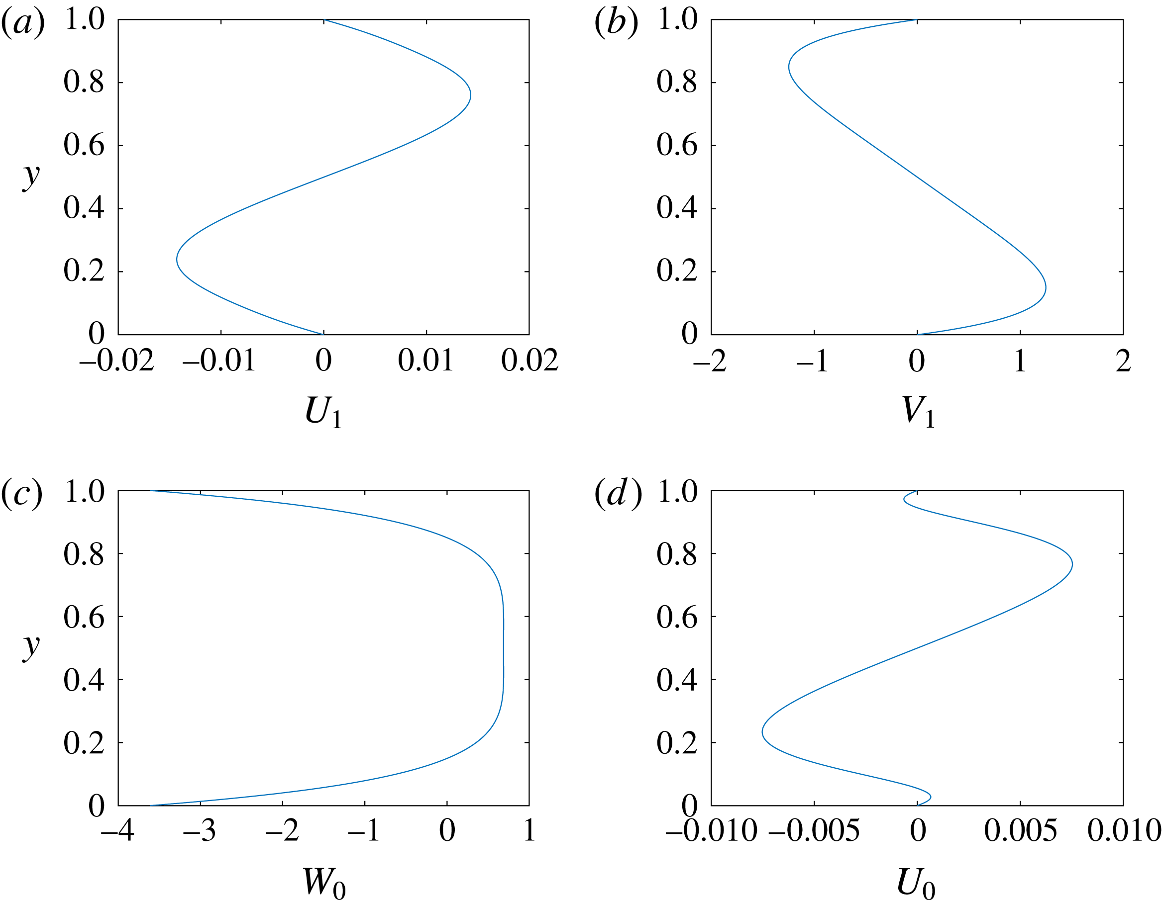
The roll–streak fundamental field and mean flow correction for the square periodic state of wavelength unity and
 $\unicode[STIX]{x1D6FC}=2.3$
. The results are shown over one period in the
 $y$
direction and the wave pressure equation will have solutions with critical layers at
 $0,1$
.

We shall first present results for two different equilibrium states we found; these correspond to
 $\unicode[STIX]{x1D6FC}=2.3$
and
 $\unicode[STIX]{x1D6FC}=3.35$
. Note that, as will be seen below, the second value of
 $\unicode[STIX]{x1D6FC}$
corresponds to a solution on the upper branch of the solution curve in
 $\unicode[STIX]{x1D70C}{-}\unicode[STIX]{x1D6FC}$
space. We restricted our attention to the case when the wavelengths in the
 $y,z$
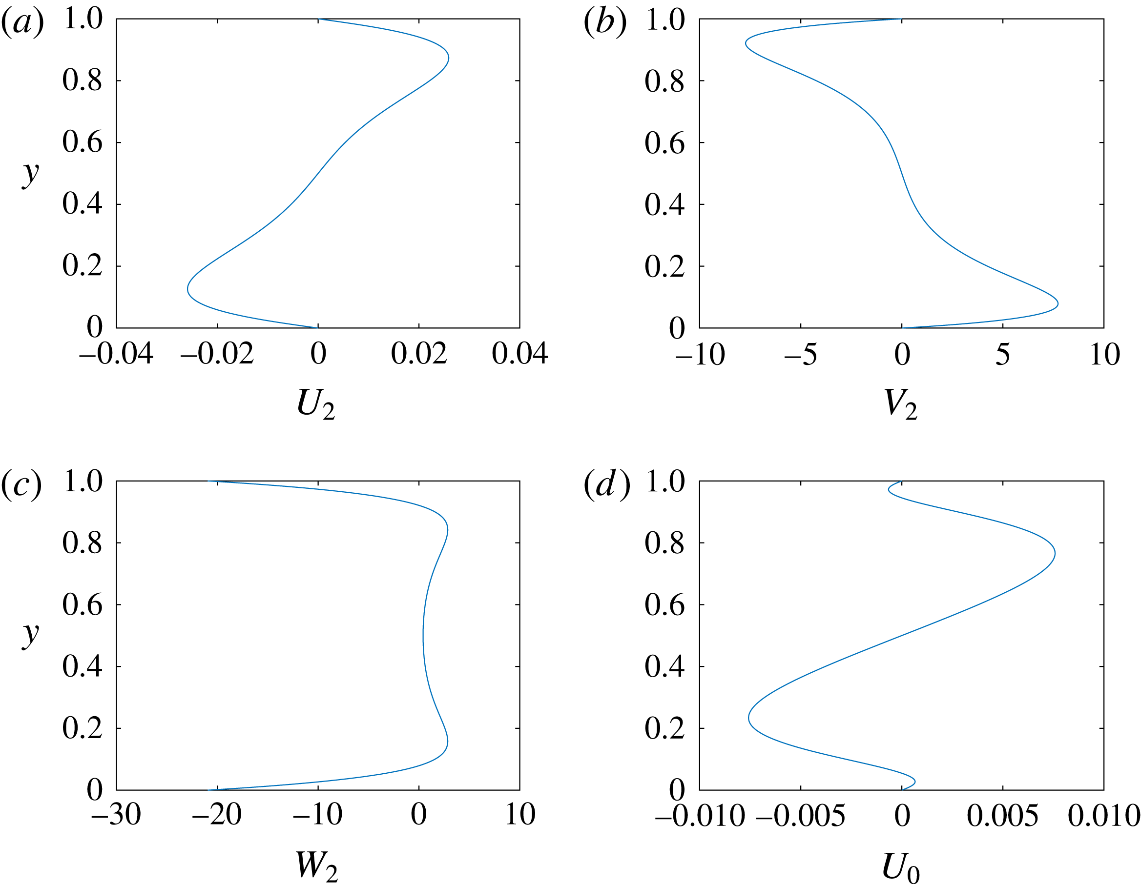
directions are both unity. Figures 4 and 5 show results for the roll–streak field for
 $\unicode[STIX]{x1D6FC}=2.3$
. We observe that the first harmonic streamwise mode
 $U_{2}$
is larger than the fundamental
 $U_{1}$
; the higher modes decrease rapidly in size. Whether there are equilibrium solutions with the fundamental dominating is an open question. Certainly our search procedures using the homotopy method were started with the dominant forcing in the fundamental, but in all cases we found that the equilibrium state deformed into one dominated by the first harmonic as
 $\unicode[STIX]{x1D6FE}$
was increased to unity. That does not rule out the possibility of modes dominated by the fundamental, but exhaustive searches failed to uncover any.
We note that the shape of the mean flow correction is such that the mean profile in the
 $y$
direction will have a ‘staircase’ shape of the type shown in figure 2 for turbulent shear flows. Thus the odd behaviour of the mean flow correction about
 $y=1/2$
will cause the total mean flow between critical layers to deform closer to a uniform-momentum flow. Note in the figures that the normal and streamwise velocity components of the roll–streak flow in fact satisfy no-slip conditions where
 $w$
does not and simply adjusts itself so that the jump in
 $W_{y}$
driven by the wave’s Reynolds stresses is satisfied. We further observe that, as required, the roll and streak fields and their derivatives with respect to
 $y$
are periodic in
 $y$
with unit period.
The roll–streak first harmonic field and mean flow correction for the square periodic state of wavelength unity and
 $\unicode[STIX]{x1D6FC}=2.3$
. The results are shown over one period in the
 $y$
direction and the wave pressure equation will have solutions with critical layers at
 $0,1$
.


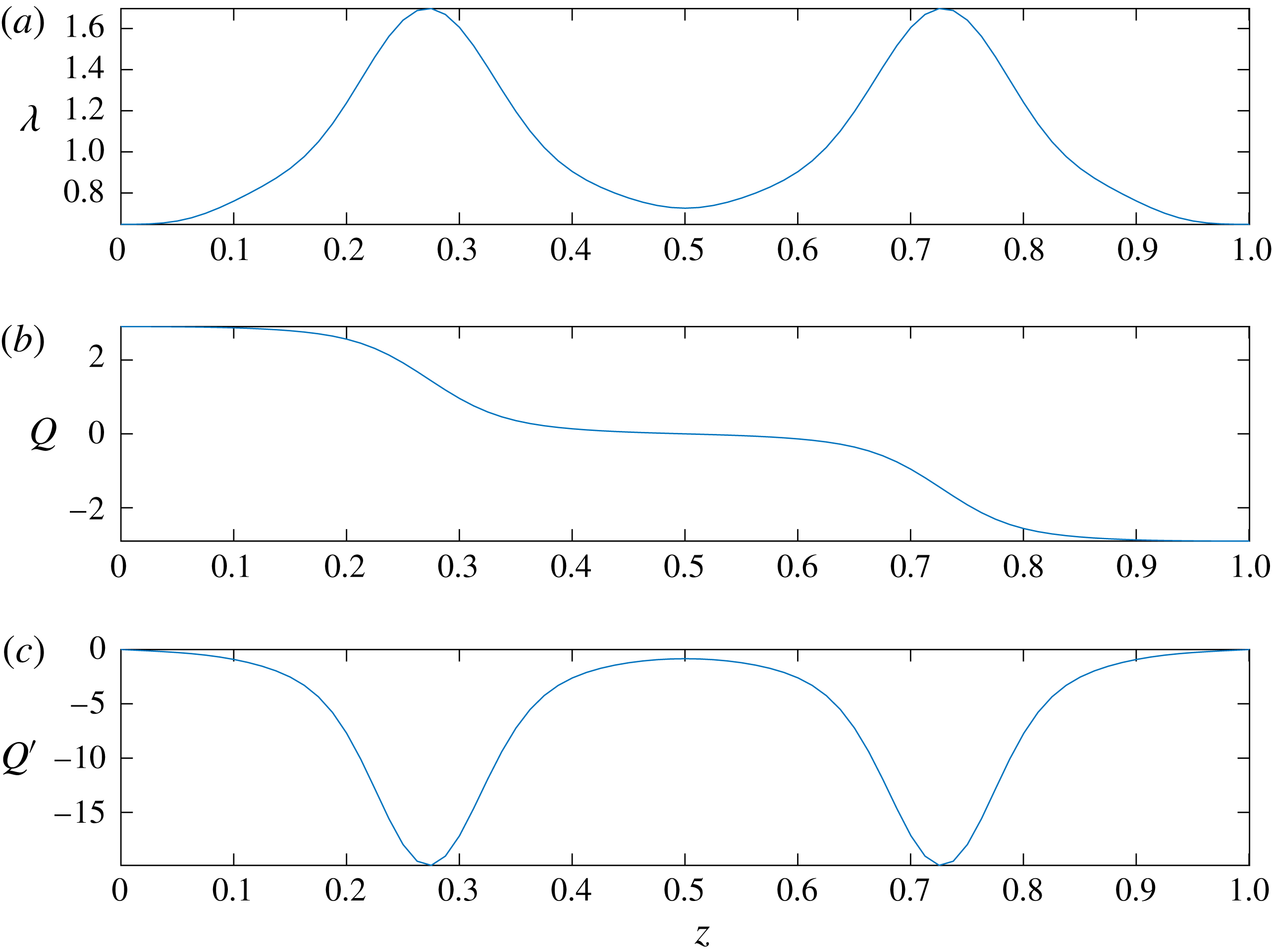
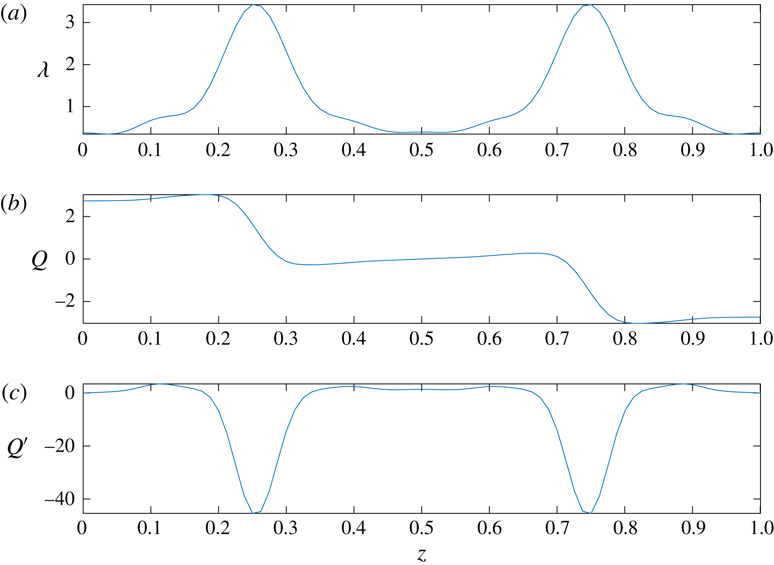
Figure 6 shows the shear stress
 $\hat{\unicode[STIX]{x1D706}}$
at the critical layer as a function of
 $z$
. Also shown in that figure are
 $Q,Q^{\prime }$
, the wave pressure field and its derivative, as functions of
 $z$
at the critical layer. Since the jump conditions are functions of
 $\unicode[STIX]{x2202}/\unicode[STIX]{x2202}z[\hat{\unicode[STIX]{x1D706}}^{-5/3}{Q^{\prime }}^{2}]$
and the
 $z$
variations of
 $Q^{\prime }$
are more pronounced than those of
 $\hat{\unicode[STIX]{x1D706}}$
, the forcing concentrates either side of the minima in figure 3(c). Moreover, the presence of two minima in
 $Q^{\prime }$
over one streak wavelength explains why the first harmonic is forced at a higher level than the fundamental. We found that this preferential forcing of the first harmonic increases as the wavenumber
 $\unicode[STIX]{x1D6FC}$
increases. Typical of the flow fields at larger
 $\unicode[STIX]{x1D6FC}$
are the results we now discuss for
 $\unicode[STIX]{x1D6FC}=3.35$
.
The roll–streak fundamental field and mean flow correction for the square periodic state of wavelength unity and
 $\unicode[STIX]{x1D6FC}=3.35$
. The results are shown over one period in the
 $y$
direction and the wave pressure equation will have solutions with critical layers at
 $0,1$
.

The roll–streak first harmonic field and mean flow correction for the square periodic state of wavelength unity and
 $\unicode[STIX]{x1D6FC}=3.35$
. The results are shown over one period in the
 $y$
direction and the wave pressure equation will have solutions with critical layers at
 $0,1$
.


Contours of constant wave pressure in the
 $y{-}Z$
plane for the case
 $\unicode[STIX]{x1D6FC}=3.35$
. Note the appearance of local maxima near the critical layer.

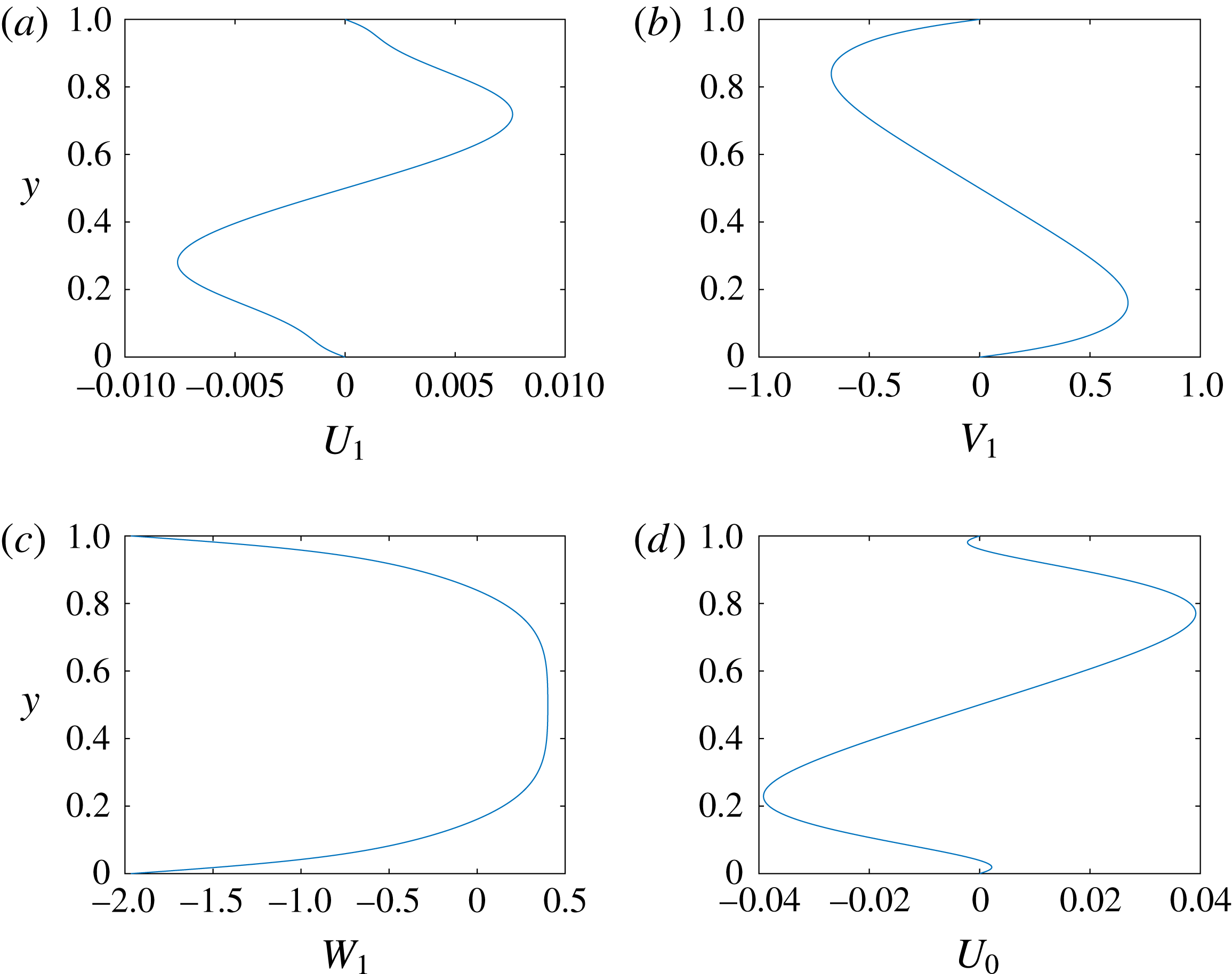
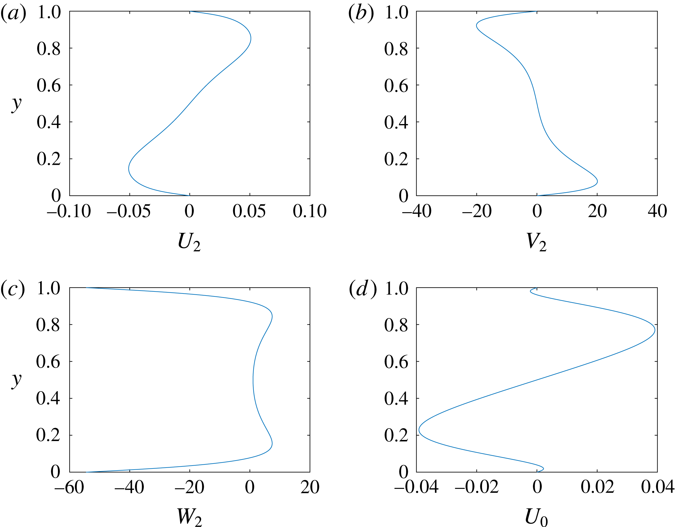
Figures 7–9 show the results corresponding to figures 4–6, respectively, but now at a value of
 $\unicode[STIX]{x1D6FC}=3.35$
. The first significant difference between the results is that the gradient of the wave pressure along the critical layer increases when
 $\unicode[STIX]{x1D6FC}$
increases. This relates to the roll stress jumps becoming more concentrated when the wavenumber increases; a similar trend can be seen in VWI states in Couette flow: see, for example, Deguchi & Hall (Reference Deguchi and Hall2014). Secondly, as a consequence of the latter effect, we note that the local minima along the critical layer of the wave pressure become pronounced. Figure 10 is a blow-up of the pressure field showing clearly the development of minima for the pressure field near to the critical layer. Note that the pressure wave field is what would one expect for a typical
 $1/2$
mirror-symmetric state. However, we see that the pressure wave field extends beyond one wavelength in the
 $y$
direction. Moreover, at the levels
 $y=\pm 1$
the normal derivative of the pressure does not vanish and so the pressure field, although displaying some of the properties of mirror-symmetric modes between rigid walls, is significantly altered by the periodicity of the streak in the
 $y$
direction. The rate of decay of the pressure field in
 $y$
is fixed by the size of the streamwise and spanwise wavenumbers. Those quantities likewise govern the rate of decay of the pressure field associated with the localised problem, so the pressure fields of the localised and periodic problems have some superficial similarities; but a more careful examination shows that there are significant differences, particular near the critical layer.
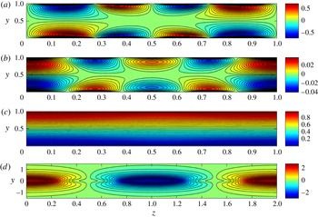
In order to further investigate the possible difference between the two cases we show in figures 11 and 12 further properties of the roll, streak and wave fields. Panel (
 $a$
) in each figure corresponds to the streamfunction associated with the roll flow and the contours denote equal values of the stream function in the unit square in the
 $y{-}z$
plane. Once again no discernible difference between the rolls is apparent and both clearly show the dominance of the first harmonic of the roll flow. Panels (
 $b$
) and (
 $c$
) show constant contours of the streak
 $U$
, and total streak
 $U+y$
in the unit square. The dominance of the second harmonic in the streak field shown is a direct result of the roll forcing having that property. Panel (
 $d$
) in each figure shows the wave field, and here we see the localisation of
 $Q^{\prime }$
mentioned above now beginning to drive smaller scale structures near
 $z=0.5,1.5$
. Note also here that we have plotted the wavefield over one full period in
 $z$
and
 $-1.5\leqslant y\leqslant 1.5$
to illustrate the decay of the wave to zero for large
 $y$
. We observe that, as could be anticipated from the asymptotic form of the decaying wave field at large
 $|y|$
,
 $Q$
is more concentrated in the
 $y$
direction at the higher value of the wavenumber.
Contours of constant stream function associated with the roll flow,
 $U(y,z)$
,
 $y+U(y,z)$
and the wave pressure
 $p(y,z)$
for the equilibrium state with
 $\unicode[STIX]{x1D6FC}=2.3$
and spanwise and vertical wavelengths of unity.

Contours of constant stream function associated with the roll flow,
 $U(y,z)$
,
 $y+U(y,z)$
and the wave pressure
 $p(y,z)$
for the equilibrium state with
 $\unicode[STIX]{x1D6FC}=3.35$
and spanwise and vertical wavelengths of unity.

The dependence of
 $\unicode[STIX]{x1D70C}$
on
 $\unicode[STIX]{x1D6FC}$
for the mirror-symmetric mode with wavelength unity in the spanwise and normal directions. The dotted curve is the small
 $\unicode[STIX]{x1D70C}$
solution
 $\unicode[STIX]{x1D70C}=\text{const.}$
 $\unicode[STIX]{x1D6FC}^{5/6}$
with the constant interpolated using the last three points on the finite
 $\unicode[STIX]{x1D6FC}$
curve.

Figure 13 shows the other equilibrium solutions we found in the
 $\unicode[STIX]{x1D6FC}{-}\unicode[STIX]{x1D70C}$
plane for unit vertical and spanwise periodicity. The continuous curve shows the range of amplitudes and wavenumbers where our iteration procedure converged. We were unable to extend our results beyond the range shown. At the lower end of the range the solutions had in effect reached an asymptotic form appropriate to the limit
 $\unicode[STIX]{x1D6FC}\rightarrow 0$
. In fact we know from Hall & Sherwin (Reference Hall and Sherwin2010) that for small
 $\unicode[STIX]{x1D6FC}$
the amplitude
 $\unicode[STIX]{x1D70C}$
goes to zero like
 $\unicode[STIX]{x1D6FC}^{5/6}$
and the arguments given in that paper leading to that result apply equally here. Indeed a log–log plot of the last four points shown shows that the small
 $\unicode[STIX]{x1D6FC}$
limit has already been achieved, so it is likely that the curve extends to smaller
 $\unicode[STIX]{x1D6FC}$
, as indicated by the dotted line. The excellent agreement between the asymptotic solution for small
 $\unicode[STIX]{x1D6FC}$
extrapolated from the first data point and the results of the full computation for
 $\unicode[STIX]{x1D6FC}$
in the range
 $(1.5,2.5)$
suggests that the equilibrium states of the full problem would simply follow the dotted red line into the origin. Note that this continuation into the origin is only possible because we have not regularised the equations as in HS or BHS; both regularisations involve keeping smaller viscous terms, and for small enough
 $\unicode[STIX]{x1D6FC}$
those terms have sufficient structure to capture the long-wavelength structure of VWI states described by Deguchi et al. (Reference Deguchi, Hall and Walton2013) in the limit
 $\unicode[STIX]{x1D6FC}\rightarrow 0$
, with
 $\unicode[STIX]{x1D6FC}R$
fixed.
The upper branch of the solutions indicated in figure 13 could not be continued to lower
 $\unicode[STIX]{x1D6FC}$
using our numerical approach. A similar difficulty arose in HS1, and the continuation of the curve above the saddle–node point was only subsequently found by limiting numerical solutions of the full Navier–Stokes equations as
 $Re$
was increased: see Deguchi & Hall (Reference Deguchi and Hall2014). Here the difficulty in continuing the curve is perhaps different since an examination of the energy in the different modes hints that there might be a bifurcation to a 1 : 4 subharmonic close to where the solution procedure fails. In fact the Deguchi & Hall (Reference Deguchi and Hall2014) quantification of the upper branch of solutions for the sinuous modes has not been done for the mirror-symmetric mode in Couette flow, so it is not clear whether the probable bifurcation is an intrinsic property of mirror-symmetric modes or whether it is special to the periodic distributions described here. The fact that when convergence was lost the solution seemed to be oscillating between two possible solutions suggests its failure was due to a bifurcation.
5.1 Evaluation of the streamwise vorticity
In order to interpret the flow field generated by the exact coherent structure derived above it is useful to consider the streamwise vorticity
 $\unicode[STIX]{x1D714}_{x}$
associated with (3.1–3.4). It suffices for us to consider the region
 $-1/2\leqslant y\leqslant 1/2$
and we see from (3.1–3.4) that away from the critical layer
 $\unicode[STIX]{x1D714}_{x}=R^{-1}(W_{z}-V_{y}+\cdots \,)$
and is therefore dominated by the roll’s streamwise vorticity. However, when the critical layer is approached the wave velocity field blows up like
 $(y-f)^{-1}$
and the critical layer within the region we are investigating has
 $f=0$
. If the critical layer is flat, only the
 $x,z$
velocity components become singular, and so the vorticity will be dominated by the contribution from the spanwise velocity component of the wave, and will rise to
 $O(R^{-1/2})$
there since the critical layer is smoothed out by viscous effects and so is of thickness
 $O(R^{-1/3})$
. From the critical layer analysis given in Hall & Sherwin (Reference Hall and Sherwin2010), we can readily show that within the critical layer the streamwise vorticity is dominated by the contribution from the spanwise component of the wave velocity field and is given by
 $$\begin{eqnarray}\displaystyle \unicode[STIX]{x1D714}_{x}=-\unicode[STIX]{x1D70C}(\unicode[STIX]{x1D6FC}\hat{\unicode[STIX]{x1D706}})^{-2/3}\text{e}^{\text{i}\unicode[STIX]{x1D6FC}x}\frac{R^{-1/2}}{(\hat{\unicode[STIX]{x1D706}}\unicode[STIX]{x1D6FC})^{2/3}}Q_{z}\frac{\unicode[STIX]{x2202}}{\unicode[STIX]{x2202}\unicode[STIX]{x1D702}}\left[\int _{0}^{\infty }\text{e}^{-\text{i}(\hat{\unicode[STIX]{x1D706}}\unicode[STIX]{x1D6FC})^{1/3}\unicode[STIX]{x1D702}s-s^{3}/3}\,\text{d}s\right]+\text{c.c.}\cdots \,. & & \displaystyle\end{eqnarray}$$
Here
 $\unicode[STIX]{x1D702}=R^{1/3}y$
is the critical layer variable and we can easily show that for large
 $\unicode[STIX]{x1D702}$
the integral behaves like
 $\unicode[STIX]{x1D702}^{-1}$
and so the vorticity decays like
 $\unicode[STIX]{x1D702}^{-2}$
, so that in a layer of depth
 $O(R^{-1/12})$
around
 $y=0$
the vorticity from the wavefield falls off to a size
 $O(R^{-1})$
consistent with that of the roll field. Note here that
 $\hat{\unicode[STIX]{x1D706}}$
is a function of
 $Z$
and we cannot separate the
 $\unicode[STIX]{x1D702}$
and
 $Z$
dependencies above. We also observe that, because only one streamwise mode contributes to the vorticity, the isosurfaces of the streamwise vorticity at any
 $\unicode[STIX]{x1D702}$
will be symmetric in
 $x$
around the
 $x$
value where a maximum is attained. Moreover, from the results shown in figure 9, it is
 $Q^{\prime }$
which dominates the shape of the spanwise variation of the streamwise vorticity in
 $Z$
. In view of the turning points of
 $Q^{\prime }$
seen in figure 9, we can anticipate that at any height contours of constant streamwise vorticity in the
 $x{-}Z$
plane will have two positive maxima in one spanwise wavelength of the streak followed by two local minima in the next wavelength. That behaviour is indicated in figure 14, where we plot surfaces of constant streamwise vorticity at different values of the critical layer variable
 $\unicode[STIX]{x1D702}$
. Note that at finite Reynolds numbers it is anticipated that the neighbouring regions become inclined to the streamwise direction to form ‘lambda’ vortices.
Finally, in this section, we note that it is expected that there will be other mirror-symmetric modes in addition to the one described above. In particular, though we could not find it using the homotopy procedure, it would be surprising if the 1 : 2 subharmonic mode did not exist. In addition to the mirror-symmetric modes we also believe that sinuous modes having no flat critical layers will exist; however, they cannot be computed by the scheme described here. Moreover, experience with VWI states in Couette flow suggests that the sinuous modes are of much larger amplitude and might therefore be the most physically relevant. In fact the solutions presented here are the first solutions of VWI equations to be computed directly without the introduction of regularisation parameters.
Surfaces enclosing regions where
 $\unicode[STIX]{x1D714}_{x}>0.8$
or
 $\unicode[STIX]{x1D714}_{x}<-0.8$
of its maximum value for the square periodic state of wavelength unity and
 $\unicode[STIX]{x1D6FC}=2.3$
.

6 VWI arrays in an arbitrary shear flows
In the previous sections we saw how periodic arrays of vortex–wave interactions can be assembled to produce exact coherent structures periodic in all three spatial dimensions and time. We now describe the extension needed to describe VWI arrays in any shear flow. In order to do so it is necessary to be more precise about the mean state in the
 $x$
direction. We assume then that it has typical speed
 $U_{0}$
and varies on a length scale
 $L$
in the normal direction. Appropriate values for these quantities will depend on the particular flow in question. If we define a Reynolds number
 $\overline{R}=U_{0}L/\unicode[STIX]{x1D708}$
then we can take the dimensionless equations of motion in the form
 $$\begin{eqnarray}\displaystyle & \displaystyle \frac{\text{D}\boldsymbol{u}}{\text{D}t}=-\unicode[STIX]{x1D735}p+\frac{1}{\overline{R}}\unicode[STIX]{x1D6FB}^{2}\boldsymbol{u}, & \displaystyle\end{eqnarray}$$
 $$\begin{eqnarray}\displaystyle & \displaystyle \unicode[STIX]{x1D735}\boldsymbol{\cdot }\boldsymbol{u}=0. & \displaystyle\end{eqnarray}$$
We are interested in coherent structures having a typical spanwise wavelength
 $\hat{\unicode[STIX]{x1D706}}^{\ast }$
and we assume this is small compared to
 $L$
, thus
 $$\begin{eqnarray}\displaystyle \hat{\unicode[STIX]{x1D706}}=\frac{\hat{\unicode[STIX]{x1D706}}^{\ast }}{L}, & & \displaystyle\end{eqnarray}$$
is a small parameter. The flows we are interested in have a mean flow
 $\overline{u}(y)$
in the
 $x$
direction together with a roll–streak flow driven by an inviscid wave system. Numerical simulations or experimental investigations of streamwise vortices in curved or essentially parallel shear flows suggest that the spanwise period of the motion is conserved as it evolves. Therefore, the spanwise wavelength will not vary in the normal direction. We also restrict attention to wave systems of fixed period in the
 $x$
direction, and so we anticipate that it is just the local normal wavelength of the array which varies in
 $y$
. The fixed wavelength conditions we apply in
 $x,z$
are at first sight at odds with the usual self-similarity assumption used in derivations of the law of the wall, where it is assumed that the flow at any
 $y$
is, apart from rescaling, the same canonical flow. Interestingly it turns out that the local VWI interaction at any
 $y$
adjusts so as in some sense to make it as self-similar as possible. For the sake of generality we allow for the presence of a constant streamwise pressure gradient driving the unperturbed flow. We will see that, though the pressure gradient can have a significant effect on the vertical structure of the periodic states, the local VWI state adjusts so as to preserve what will turn out to be a canonical form for the mean flow.
The more general variation of the mean state with
 $y$
means that exact triply periodic coherent structures must adjust to the local flow conditions, which means that the local wavenumber in the normal direction must vary with
 $y$
. We can account for such a variation by introducing the phase function
 $\unicode[STIX]{x1D6F7}$
defined by
 $$\begin{eqnarray}\displaystyle \unicode[STIX]{x1D6F7}=\frac{\unicode[STIX]{x1D703}(y)}{\hat{\unicode[STIX]{x1D706}}}, & & \displaystyle\end{eqnarray}$$
and we will seek a structure which is periodic in
 $\unicode[STIX]{x1D6F7}$
with period unity. Note from (6.4) that periodicity in
 $\unicode[STIX]{x1D6F7}$
implies only local periodicity in
 $y$
. Thus we are seeking a nonlinear Wentzel–Kramers–Brillouin–Jeffreys (WKBJ) or ray theory solution where the local periodicity in the normal direction adjusts to the local mean flow properties.
In the usual arguments leading to the law of the wall, self-similarity in the three spatial directions is invoked. Thus it is assumed that apart from identical changes in length scale in the three directions the flow is identical. Thus it appears at first sight that the fact that we are only allowing for slow variations in the
 $y$
direction precludes us obtaining a structure consistent with the classical ‘self-similar’ view. That is not the case for the following reasons.
Firstly we will see below that the wave part of the distributed interaction feels only the local flow structure, the wavespeed is fixed by making it propagate downstream with the local streamwise mean velocity, but the streamwise wavenumber can be a function of
 $y$
. This is because the wave is localised near its critical layer, so we are not discussing a single wave with varying wavenumber but an infinite sum of waves of possibly differing streamwise wavenumbers. We are therefore at liberty to allow choose the wavenumber so that the flow is self-similar in
 $x$
and
 $z$
.
Secondly we note that we fix the spanwise wavenumber to be that associated with the spanwise box width used in the computations. In exactly the same way as is done in Navier–Stokes calculations, we could begin with a box width many times the spanwise wavelength and allow the energy to migrate across spanwise wavenumbers as
 $y$
varies. That increases enormously the size of the computation, and so here we restrict attention to the case when the box width and spanwise wavelength coincide. However, the much bigger scale computation for the more general case would, as found in Navier–Stokes simulations, allow the distributed structure to have self-similarity in all three directions.
We define ‘fast’ variables
 $X=x/\hat{\unicode[STIX]{x1D706}}$
,
 $Z=\unicode[STIX]{x1D6FD}z/\hat{\unicode[STIX]{x1D706}}$
,
 $T=t/\hat{\unicode[STIX]{x1D706}}$
. In § 3 we saw how the introduction of an infinite sum of inviscid waves of wavenumber
 $\unicode[STIX]{x1D6FC}$
riding on the shear flow with critical layers separated by a constant distance could drive a non-zero roll–streak flow also periodic in the normal direction. But now the periodicity is in terms of the fast
 $\unicode[STIX]{x1D6F7}$
variable, so we will consider an infinite sum of waves of the same streamwise wavenumber and with wavespeeds given by the local streamwise mean velocity at
 $y=y_{n}$
where
 $$\begin{eqnarray}\displaystyle \unicode[STIX]{x1D6F7}=\unicode[STIX]{x1D6F7}_{n}=\frac{\unicode[STIX]{x1D703}(y_{n})}{\hat{\unicode[STIX]{x1D706}}}=\unicode[STIX]{x1D6F7}^{\ast }+n. & & \displaystyle\end{eqnarray}$$
Here
 $\unicode[STIX]{x1D6F7}^{\ast }$
is a constant and
 $n=0,\pm 1,\pm 2,\ldots \,$
.
Let us consider the form of the operator
 $\unicode[STIX]{x2202}/\unicode[STIX]{x2202}t+\overline{u}(\unicode[STIX]{x2202}/\unicode[STIX]{x2202}x)$
which will appear in the linearised equations for the waves. If we focus on the wave with critical layer at
 $\unicode[STIX]{x1D6F7}_{n}$
and write
 $$\begin{eqnarray}\unicode[STIX]{x1D6F7}=\unicode[STIX]{x1D6F7}_{n}+\unicode[STIX]{x1D719}\end{eqnarray}$$
then near
 $y_{n}$
 $$\begin{eqnarray}\displaystyle y-y_{n}=\frac{\hat{\unicode[STIX]{x1D706}}\unicode[STIX]{x1D719}}{\unicode[STIX]{x1D703}^{\prime }(y_{n})}+\cdots \,, & & \displaystyle\end{eqnarray}$$
so that for the wave proportional to
 $\text{e}^{\text{i}\unicode[STIX]{x1D6FC}[X-\overline{u}(y_{n})T]}$
we have
 $$\begin{eqnarray}\displaystyle \frac{\unicode[STIX]{x2202}}{\unicode[STIX]{x2202}t}+\overline{u}\frac{\unicode[STIX]{x2202}}{\unicode[STIX]{x2202}x}=\text{i}\unicode[STIX]{x1D6FC}\left[\frac{\overline{u}^{\prime }(y_{n})}{\unicode[STIX]{x1D703}^{\prime }(y_{n})}\unicode[STIX]{x1D719}+\cdots \cdots \,\right]\simeq \text{i}\unicode[STIX]{x1D6FC}\left[\frac{\overline{u}^{\prime }(y)}{\unicode[STIX]{x1D703}^{\prime }(y)}\unicode[STIX]{x1D719}+\cdots \cdots \,\right], & & \displaystyle\end{eqnarray}$$
and we can replace
 $y_{n}$
by
 $y$
in
 $\overline{u}^{\prime }(y_{n})/\unicode[STIX]{x1D703}^{\prime }(y_{n})$
because
 $y-y_{n}=O(\hat{\unicode[STIX]{x1D706}}).$
If we modify the streamwise velocity component by adding on a ‘streak’ term at order
 $\hat{\unicode[STIX]{x1D706}}$
then the above result suggests that, in order to reduce the pressure wave equation to a form independent of the slow variable
 $y$
, the streak should also be proportional to
 $\overline{u}^{\prime }/\unicode[STIX]{x1D703}^{\prime }$
.
Figure 15 is a sketch of the type of array of VWI states we are considering. The critical layers are a distance
 $O(\hat{\unicode[STIX]{x1D706}})$
apart if we work in terms of
 $y$
. On the other hand if plotted in terms of
 $\unicode[STIX]{x1D6F7}$
the critical layers are unit distance apart. Within each critical layer the Reynolds stresses associated with the self-interaction of the wave concentrated there generate a stress jump in the roll field. In terms of the fast variable
 $\unicode[STIX]{x1D6F7}$
the induced stress jumps are periodic with unit wavelength, thereby sustaining the local periodic roll–streak field.
Schematic showing the distribution of VWI states for an arbitrary shear flow. The orange regions denote the thin viscous critical layers needed to regularise the inviscid wave operator there and within which the appropriate local stress jumps on the roll are generated. Note that the layers are a distance
 $O(\hat{\unicode[STIX]{x1D706}})$
apart but the separation in each case is unity in terms of the phase variable
 $\unicode[STIX]{x1D6F7}$
.

Now suppose we look for a roll–streak flow of the form
 $$\begin{eqnarray}\displaystyle & \displaystyle u=\overline{u}(y)+\hat{\unicode[STIX]{x1D706}}\frac{\overline{u}^{\prime }}{\unicode[STIX]{x1D703}^{\prime }}[U_{1}^{\dagger }(\unicode[STIX]{x1D6F7},Z,y)+\hat{\unicode[STIX]{x1D706}}U_{2}^{\dagger }(\unicode[STIX]{x1D6F7},Z,y)+\cdots \,], & \displaystyle\end{eqnarray}$$
 $$\begin{eqnarray}\displaystyle & \displaystyle v=\frac{\unicode[STIX]{x1D703}^{\prime }}{\hat{\unicode[STIX]{x1D706}}\overline{R}}[V_{1}^{\dagger }(\unicode[STIX]{x1D6F7},Z,y)+\hat{\unicode[STIX]{x1D706}}V_{2}^{\dagger }(\unicode[STIX]{x1D6F7},Z,y)+\cdots \,], & \displaystyle\end{eqnarray}$$
 $$\begin{eqnarray}\displaystyle & \displaystyle w=\frac{\unicode[STIX]{x1D703}^{\prime }}{\hat{\unicode[STIX]{x1D706}}\overline{R}}[W_{1}^{\dagger }(\unicode[STIX]{x1D6F7},Z,y)+\hat{\unicode[STIX]{x1D706}}W_{2}^{\dagger }(\unicode[STIX]{x1D6F7},Z,y)+\cdots \,], & \displaystyle\end{eqnarray}$$
 $$\begin{eqnarray}\displaystyle & \displaystyle p=-\overline{p}(x)+\frac{{\unicode[STIX]{x1D703}^{\prime }}^{2}\overline{u}^{\prime }}{\hat{\unicode[STIX]{x1D706}}^{2}\overline{R}^{2}}[P_{1}^{\dagger }(\unicode[STIX]{x1D6F7},Z,y)+\hat{\unicode[STIX]{x1D706}}P_{2}^{\dagger }(\unicode[STIX]{x1D6F7},Z,y)+\cdots \,]. & \displaystyle\end{eqnarray}$$
Here
 ${\overline{p}_{x}}^{\prime }$
is now the streamwise pressure gradient and the factor
 $\hat{\unicode[STIX]{x1D706}}^{2}\overline{R}$
is assumed large since if it becomes
 $O(1)$
the disturbances are operating on the Kolmogorov length scale and the VWI reduction of the interaction equations is not possible. The quantity
 $\hat{\unicode[STIX]{x1D706}}^{2}\overline{R}$
is the effective local Reynolds number based on
 $\hat{\unicode[STIX]{x1D706}}^{\ast }$
and the local mean flow rather than
 $L,U_{0}$
. That is why we have assumed the relative scaling shown above for the terms proportional to
 $U_{1}^{\dagger },V_{1}^{\dagger }$
. Based on the discussion beneath (6.8) we have, for convenience, inserted the factor
 $\overline{u}^{\prime }/\unicode[STIX]{x1D703}^{\prime }$
in the
 $O(\hat{\unicode[STIX]{x1D706}})$
term in (6.9). Once we anticipate that the spanwise varying part of the streamwise velocity component should be proportional to
 $\overline{u}^{\prime }/\unicode[STIX]{x1D703}^{\prime }$
the corresponding scalings shown for the other two velocity components and pressure follow.
The leading-order approximation to the equations of motion for the streamwise averaged part of the flow is
 $$\begin{eqnarray}\displaystyle & \displaystyle V_{1}^{\dagger }+V_{1}^{\dagger }U_{1\unicode[STIX]{x1D6F7}}^{\dagger }+\frac{\unicode[STIX]{x1D6FD}}{\unicode[STIX]{x1D703}^{\prime }}W_{1}^{\dagger }U_{1Z}^{\dagger }=\left[\frac{\unicode[STIX]{x2202}^{2}}{\unicode[STIX]{x2202}\unicode[STIX]{x1D6F7}^{2}}+\frac{\unicode[STIX]{x1D6FD}^{2}}{{\unicode[STIX]{x1D703}^{\prime }}^{2}}\frac{\unicode[STIX]{x2202}^{2}}{\unicode[STIX]{x2202}Z^{2}}\right]U_{1,}^{\dagger } & \displaystyle\end{eqnarray}$$
 $$\begin{eqnarray}\displaystyle & \displaystyle V_{1}^{\dagger }V_{1\unicode[STIX]{x1D6F7}}^{\dagger }+\frac{\unicode[STIX]{x1D6FD}}{\unicode[STIX]{x1D703}^{\prime }}W_{1}^{\dagger }V_{1Z}^{\dagger }=-P_{1\unicode[STIX]{x1D6F7}}^{\dagger }+\left[\frac{\unicode[STIX]{x2202}^{2}}{\unicode[STIX]{x2202}\unicode[STIX]{x1D6F7}^{2}}+\frac{\unicode[STIX]{x1D6FD}^{2}}{{\unicode[STIX]{x1D703}^{\prime }}^{2}}\frac{\unicode[STIX]{x2202}^{2}}{\unicode[STIX]{x2202}Z^{2}}\right]V_{1,}^{\dagger } & \displaystyle\end{eqnarray}$$
 $$\begin{eqnarray}\displaystyle & \displaystyle V_{1}^{\dagger }W_{1\unicode[STIX]{x1D6F7}}^{\dagger }+\frac{\unicode[STIX]{x1D6FD}}{\unicode[STIX]{x1D703}^{\prime }}W_{1}^{\dagger }W_{1Z}^{\dagger }=-\frac{\unicode[STIX]{x1D6FD}}{\unicode[STIX]{x1D703}^{\prime }}P_{1Z}^{\dagger }+\left[\frac{\unicode[STIX]{x2202}^{2}}{\unicode[STIX]{x2202}\unicode[STIX]{x1D6F7}^{2}}+\frac{\unicode[STIX]{x1D6FD}^{2}}{{\unicode[STIX]{x1D703}^{\prime }}^{2}}\frac{\unicode[STIX]{x2202}^{2}}{\unicode[STIX]{x2202}Z^{2}}\right]W_{1,}^{\dagger } & \displaystyle\end{eqnarray}$$
 $$\begin{eqnarray}\displaystyle & \displaystyle V_{1\unicode[STIX]{x1D6F7}}^{\dagger }+\frac{\unicode[STIX]{x1D6FD}}{\unicode[STIX]{x1D703}^{\prime }}W_{1Z}^{\dagger }=0. & \displaystyle\end{eqnarray}$$
Apart from the factor
 $1/\unicode[STIX]{x1D703}^{\prime }$
premultiplying each
 $Z$
derivative and with
 $y$
and
 $\unicode[STIX]{x1D719}$
interchanged these equations are simply (3.5)–(3.8) so that the only slow dependence of the equations is through the local wavenumber
 $\unicode[STIX]{x1D6FD}/\unicode[STIX]{x1D703}^{\prime }$
. The equations must be solved subject to periodicity in the
 $Z$
direction with wavelength
 $2\unicode[STIX]{x03C0}$
. Once again in the absence of any wave forcing there will be no nonlinear equilibrium solution of these equations.
We saw earlier that the wave system driving the equilibrium state takes the form of an infinite sum of waves with the same downstream wavenumber
 $\unicode[STIX]{x1D6FC}$
and with wavespeeds
 $\overline{u}(y_{n})$
, where
 $y_{n}$
is defined by (6.5). This is an important difference from the uniform shear case since now the waves which drive the roll flows will have their frequencies an integer multiple of some factor, but that factor will change slowly in
 $y$
. Thus the time period of the contributing waves at any depth will be a function of depth. Note that this is subtly different from having a single wave with its frequency a function of position; this is because the contributing waves must convect with the local basic flow in order to drive the roll system locally. In other problems, such as two-dimensional Tollmien–Schlichting waves propagating in a boundary layer, a phase function depending on time must be introduced to describe a similar effect because the same wave provides the nonlinear feedback at all locations; see, for example, Hall (Reference Hall1995). We now perturb the roll–streak system described by (6.13)–(6.16) to a small-amplitude inviscid wave system. If, for example, we let
 $\tilde{p}$
denote the wave pressure to be added to (6.12) we write
 $$\begin{eqnarray}\displaystyle \tilde{p}=\frac{\hat{\unicode[STIX]{x1D706}}^{2}\unicode[STIX]{x1D70C}(y_{n})(\overline{u}^{\prime }(y_{n}))^{5/6}(\unicode[STIX]{x1D703}^{\prime }(y_{n}))^{1/3}}{(\hat{\unicode[STIX]{x1D706}}^{2}\overline{R})^{7/6}}\displaystyle \mathop{\sum }_{-\infty }^{\infty }\text{e}^{\text{i}\unicode[STIX]{x1D6FC}[X-\overline{u}(y_{n})T]}\widetilde{p}_{n}(\unicode[STIX]{x1D6F7}-\unicode[STIX]{x1D6F7}_{n},z,y)+\text{c.c.}, & & \displaystyle\end{eqnarray}$$
where
 $\unicode[STIX]{x1D70C}(y_{n})$
is the amplitude of the ‘
 $n$
th’ wave and the factors dependent on
 $\unicode[STIX]{x1D703}^{\prime },\overline{U}^{\prime }$
have been introduced in order to facilitate comparison with the uniform shear case. The equation to describe each wave is found by expanding the normal variations in terms of
 $\unicode[STIX]{x1D719}$
. Each wave decays to zero exponentially for large values of the modulus of
 $\unicode[STIX]{x1D719}=\unicode[STIX]{x1D6F7}-\unicode[STIX]{x1D6F7}_{n}$
but reinforces the roll–streak structure within its own critical layer. Furthermore, because
 $y-y_{n}$
is
 $O(\hat{\unicode[STIX]{x1D706}})$
, we can replace
 $\unicode[STIX]{x1D70C}(y_{n})$
by
 $\unicode[STIX]{x1D70C}(y)$
above and in what follows.
The wave pressure equation for the
 $n$
th wave is
 $$\begin{eqnarray}\displaystyle \left(\frac{\widetilde{p}_{n\unicode[STIX]{x1D719}}}{[\unicode[STIX]{x1D719}+U_{1}^{\dagger }]^{2}}\right)_{\unicode[STIX]{x1D719}}+\frac{\unicode[STIX]{x1D6FD}^{2}}{{\unicode[STIX]{x1D703}^{\prime }}^{2}}\left(\frac{\widetilde{p}_{nz}}{[\unicode[STIX]{x1D719}+U_{1}^{\dagger }]^{2}}\right)_{z}-\frac{\unicode[STIX]{x1D6FC}^{2}\widetilde{p}_{n}}{{\unicode[STIX]{x1D703}^{\prime }}^{2}[\unicode[STIX]{x1D719}+U_{1}^{\dagger }]^{2}}=0, & & \displaystyle\end{eqnarray}$$
which must be solved subject to
 $$\begin{eqnarray}\displaystyle \widetilde{p}_{n}\rightarrow 0,\quad |\unicode[STIX]{x1D719}|\rightarrow \infty ,\quad \widetilde{p}_{n}(\unicode[STIX]{x1D719},Z)=\widetilde{p}_{n}(\unicode[STIX]{x1D719},Z+2\unicode[STIX]{x03C0}). & & \displaystyle\end{eqnarray}$$
Thus, once again, apart from a prefactor
 $1/\unicode[STIX]{x1D703}^{\prime }(y_{n})$
multiplying each
 $Z$
derivative and
 $\unicode[STIX]{x1D6FC}$
, we have the wave pressure equation (3.9) of the uniform shear case. The interaction of each wave with itself produces jump conditions on the tangential roll stresses at
 $\unicode[STIX]{x1D6F7}-\unicode[STIX]{x1D6F7}_{n}=\unicode[STIX]{x1D719}=0$
. We restrict attention to mirror-symmetric modes which have flat critical layers and so
 $u_{1},v_{1},w_{1},u_{1\unicode[STIX]{x1D719}},v_{1\unicode[STIX]{x1D719}}$
are continuous across the critical layer whilst
 $$\begin{eqnarray}\displaystyle \left[\frac{\unicode[STIX]{x2202}W_{1}^{\dagger }}{\unicode[STIX]{x2202}\unicode[STIX]{x1D719}}\right]_{-}^{+}=n_{0}\unicode[STIX]{x1D6FD}^{3}\unicode[STIX]{x1D70C}^{2}(y_{n})\left(\frac{\unicode[STIX]{x1D6FC}}{\unicode[STIX]{x1D703}^{\prime }(y_{n})}\right)^{-5/3}(\unicode[STIX]{x1D703}^{\prime }(y_{n}))^{-3}\frac{\unicode[STIX]{x2202}}{\unicode[STIX]{x2202}Z}(\{1+U_{1\unicode[STIX]{x1D719}}^{\dagger }\}^{-5/3}|\widetilde{Q}_{nZ}|^{2}), & & \displaystyle\end{eqnarray}$$
where
 $\widetilde{Q}_{n}$
is
 $\widetilde{p}_{n}$
evaluated on the critical layer where
 $\unicode[STIX]{x1D6F7}-\unicode[STIX]{x1D6F7}_{n}=\unicode[STIX]{x1D719}=0$
.
The above discussion for the
 $n$
th wave applies to all the other waves, and so the upshot then is that the roll–streak system is driven by the jump condition (6.20) but now with
 $y_{n}$
replaced by
 $y$
; we can of course do that because
 $y-y_{n}$
is
 $O(\hat{\unicode[STIX]{x1D706}})$
. The local roll–streak–wave problem is now, apart from the prefactor
 $1/\unicode[STIX]{x1D703}^{\prime }(y_{n})$
multiplying each
 $Z$
derivative or term proportional to
 $\unicode[STIX]{x1D6FC}$
, identical to that found for the uniform shear case and so, using (3.16) the local wave amplitude must satisfy
 $$\begin{eqnarray}\displaystyle \unicode[STIX]{x1D70C}(y)={\mathcal{F}}\left(\frac{\unicode[STIX]{x1D6FC}}{\unicode[STIX]{x1D703}^{\prime }(y)},\frac{\unicode[STIX]{x1D6FD}}{\unicode[STIX]{x1D703}^{\prime }(y)}\right). & & \displaystyle\end{eqnarray}$$
Thus the local values in
 $y$
of the effective streamwise and spanwise wavenumbers of the equivalent periodic problem in a uniform shear flow become
 $\unicode[STIX]{x1D6FC}/\unicode[STIX]{x1D703}^{\prime }(y)$
,
 $\unicode[STIX]{x1D6FD}/\unicode[STIX]{x1D703}^{\prime }(y)$
, respectively. If
 $\bar{u},\unicode[STIX]{x1D703}$
are known for given values of
 $\unicode[STIX]{x1D6FC},\unicode[STIX]{x1D6FD}$
the eigenrelation (6.21) gives the local wave amplitude needed to sustain the local triply periodic VWI state. The functional form of
 $U_{1}^{\dagger },V_{1}^{\dagger },W_{1}^{\dagger },P_{1}^{\dagger }$
is revealed by comparison of the local nonlinear eigenvalue problem with that of the uniform shear periodic problem of § 3. It follows from (6.13)–(6.20) that these quantities only depend on
 $y$
through the local wavenumbers
 $\unicode[STIX]{x1D6FC}/\unicode[STIX]{x1D703}^{\prime }$
,
 $\unicode[STIX]{x1D6FD}/\unicode[STIX]{x1D703}^{\prime }$
, so that, for example,
 $$\begin{eqnarray}\displaystyle U_{1}^{\dagger }={\mathcal{U}}\left(\frac{\unicode[STIX]{x1D6FC}}{\unicode[STIX]{x1D703}^{\prime }},\frac{\unicode[STIX]{x1D6FD}}{\unicode[STIX]{x1D703}^{\prime }},\unicode[STIX]{x1D719},Z\right). & & \displaystyle\end{eqnarray}$$
It is crucial at this stage to observe that
 $U_{1}^{\dagger }$
and
 $V_{1}^{\dagger }$
are independent of
 $\overline{u}^{\prime }$
because of the factors we introduced into the
 $O(\hat{\unicode[STIX]{x1D706}})$
terms in (6.9)–(6.10). At first sight it might appear then that the slowly varying triply periodic VWI states have been completely determined, but of course, given
 $\unicode[STIX]{x1D6FC},\unicode[STIX]{x1D6FD}$
, the local nonlinear eigenvalue fixes the wave amplitude
 $\unicode[STIX]{x1D70C}$
in terms of
 $\unicode[STIX]{x1D6FC}/\unicode[STIX]{x1D703}^{\prime }$
,
 $\unicode[STIX]{x1D6FD}/\unicode[STIX]{x1D703}^{\prime }$
at the local values of
 $\unicode[STIX]{x1D703}^{\prime }$
and
 $\overline{u}^{\prime }$
, and these functions remain unknown. Note that for given
 $\unicode[STIX]{x1D6FC},\unicode[STIX]{x1D6FD}$
the equivalent periodic infinite uniform shear problem with wavenumbers
 $\unicode[STIX]{x1D6FC}/\unicode[STIX]{x1D703}^{\prime }$
,
 $\unicode[STIX]{x1D6FD}/\unicode[STIX]{x1D703}^{\prime }$
has the streamwise and spanwise wavenumbers varying but with their ratio held fixed.
In fact, as is generally the case for linear or nonlinear WKBJ expansions, there will be a further condition relating these quantities at higher order. We might expect that condition arises because of the translational invariance of our solution in the
 $\unicode[STIX]{x1D6F7}$
variable; see, for example, Hall (Reference Hall1995). But the translational invariance associated with that case cannot apply here because the
 $\unicode[STIX]{x1D6F7}$
dependence is effectively pinned by the stress jumps induced by the wave system. Indeed the wave system drives, periodically spaced in
 $\unicode[STIX]{x1D6F7}$
, discontinuities in the slope of
 ${W_{1}}^{\dagger }$
so we cannot move the whole pattern upwards by an arbitrarily small amount and do a local expansion to deduce that the linearised form of the leading order nonlinear problem must have a solution. Usually it is the existence of a solution of that linearised problem which necessitates the imposition of a solvability problem on the next-order problem in the nonlinear WKBJ expansion procedure. Thus when we write down the next-order approximation to the equations of motion based on the expansion (6.9)–(6.12) we will obtain a linear system of equations which will couple to the next-order form of the wave pressure equation and that system will automatically have a solution.
In particular, the next-order approximation to the streamwise momentum and continuity equations yields
 $$\begin{eqnarray}\displaystyle & \displaystyle V_{2}^{\dagger }+V_{2}^{\dagger }U_{1\unicode[STIX]{x1D6F7}}^{\dagger }+\frac{\unicode[STIX]{x1D6FD}}{\unicode[STIX]{x1D703}^{\prime }}W_{2}^{\dagger }U_{1Z}^{\dagger }+V_{1}^{\dagger }U_{2\unicode[STIX]{x1D6F7}}^{\dagger }+\frac{\unicode[STIX]{x1D6FD}}{\unicode[STIX]{x1D703}^{\prime }}W_{1}^{\dagger }U_{2Z}^{\dagger }=\left[\frac{\unicode[STIX]{x2202}^{2}}{\unicode[STIX]{x2202}\unicode[STIX]{x1D6F7}^{2}}+\frac{\unicode[STIX]{x1D6FD}^{2}}{{\unicode[STIX]{x1D703}^{\prime }}^{2}}\frac{\unicode[STIX]{x2202}^{2}}{\unicode[STIX]{x2202}Z^{2}}\right]U_{2,}^{\dagger }+S_{1} & \displaystyle\end{eqnarray}$$
 $$\begin{eqnarray}\displaystyle & \displaystyle V_{2\unicode[STIX]{x1D6F7}}^{\dagger }+\frac{\unicode[STIX]{x1D6FD}}{\unicode[STIX]{x1D703}^{\prime }}W_{2Z}^{\dagger }=S_{2}, & \displaystyle\end{eqnarray}$$
where the inhomogeneous terms
 $S_{1}$
is given by
 $$\begin{eqnarray}\overline{u}^{\prime }\unicode[STIX]{x1D703}^{\prime }S_{1}=\frac{\overline{u}^{\prime \prime }-\overline{p}_{x}}{\overline{u}^{\prime }\unicode[STIX]{x1D703}^{\prime }}+\left[\overline{u}^{\prime \prime }-\frac{\overline{u}^{\prime }\unicode[STIX]{x1D703}^{\prime \prime }}{\unicode[STIX]{x1D703}^{\prime }}\right]V_{1}^{\dagger }U_{1}^{\dagger }+\overline{u}^{\prime }V_{1}^{\dagger }U_{1y}^{\dagger }+\left(\left[2\overline{u}^{\prime }-\frac{\overline{u}^{\prime }\unicode[STIX]{x1D703}^{\prime \prime }}{\unicode[STIX]{x1D703}^{\prime }}\right]\frac{\unicode[STIX]{x2202}}{\unicode[STIX]{x2202}\unicode[STIX]{x1D6F7}}+2\overline{u}^{\prime }\frac{\unicode[STIX]{x2202}^{2}}{\unicode[STIX]{x2202}\unicode[STIX]{x1D6F7}\unicode[STIX]{x2202}y}\right)U_{1}^{\dagger },\end{eqnarray}$$
and
 $$\begin{eqnarray}S_{2}=\frac{\unicode[STIX]{x1D703}^{\prime \prime }}{{\unicode[STIX]{x1D703}^{\prime }}^{2}}V_{1}^{\dagger }-\frac{1}{\unicode[STIX]{x1D703}^{\prime }}V_{1y}^{\dagger }.\end{eqnarray}$$
We are seeking a structure periodic in both
 $\unicode[STIX]{x1D6F7}$
and
 $Z$
, so if we integrate (6.23) over
 $A$
defined by
 $0<y<1,0<Z<2\unicode[STIX]{x03C0}$
and use (6.16), (6.23) after integration by parts we deduce that
 $$\begin{eqnarray}\displaystyle \overline{u}^{\prime \prime }+[(\overline{u}^{\prime }\unicode[STIX]{x1D70E})]^{\prime }=\overline{p}_{x}, & & \displaystyle\end{eqnarray}$$
where a dash denotes a derivative with respect to
 $y$
and
 $$\begin{eqnarray}\displaystyle \unicode[STIX]{x1D70E}=-\frac{1}{2\unicode[STIX]{x03C0}}\iint _{A}{\mathcal{U}}{\mathcal{V}}\,\text{d}y\,\text{d}z & & \displaystyle\end{eqnarray}$$
is a function of
 $y$
only through the dependence of the roll–streak field on
 $\unicode[STIX]{x1D703}^{\prime }(y)$
. Here the integral is taken over the rectangle
 $A$
and
 ${\mathcal{U}},{\mathcal{V}}$
are the infinite uniform shear periodic streak and roll fields for wavenumbers
 $\unicode[STIX]{x1D6FC}/\unicode[STIX]{x1D703}^{\prime }$
,
 $\unicode[STIX]{x1D6FD}/\unicode[STIX]{x1D703}^{\prime }$
in the
 $x,Z$
directions.
The slow evolution equation (6.27) involving the mean flow and the phase function
 $\unicode[STIX]{x1D703}$
has a striking similarity with (1.1), the equation for the mean part of a turbulent flow. In fact (6.27) can be deduced directly from (1.1). We recall that in (1.1) a bar denotes an average over the streamwise and spanwise directions. Since (1.1) is exact we can apply it to the velocity field given in (6.9)–(6.10); note the contribution from the wave part of the flow is a higher-order effect and the leading-order average of the term
 $uv$
in (1.1) is the average in
 $Z$
of the leading-order roll multiplied by the leading-order streak. Interestingly the effect of the wave on the mean manifests itself through the roll which is driven by the wave-induced stress jump. In the structure proposed here we have local periodicity in
 $\unicode[STIX]{x1D6F7}$
, so averaging (1.1) over the fast variable
 $\unicode[STIX]{x1D6F7}$
produces exactly (6.27). Thus the slow dynamics of the distributed vortex–wave state is fixed by the usual turbulent mean equation, except that we now have an explicit expression for the ‘closure’ problem between the small scale flow and the mean! So (6.27) can be viewed as a simplification of (1.1) which takes out the small-scale dependence of the mean flow. The above discussion applies equally to all distributed VWI arrays and does not depend on the mirror-symmetry properties of the particular case we investigated in § 5. Note that though our restricted investigations discussed in § 5 were all for mirror-symmetric states the analysis we have given in this section applies to any class of VWI state.
7 The slow dynamics equation and the log law
Here we will discuss the possible relevance of the types of distributed vortex arrays described in the previous section. It is now generally accepted the SSP/VWI mechanism is responsible for the near-wall streaky behaviour found in wall-bounded shear flows. Though there have been numerous numerical simulations capable of quantifying some flow properties of the flow in the log layer there has been no attempt to use the SSP/VWI framework to describe the flow there. However, we know from simulations that the log layer depth is large compared to the streamwise and spanwise wavenumbers implicated in the sustaining mechanism. As pointed out earlier in this paper, a sequence of VWI states localised in the wall normal direction simply produce a relatively small jump in the mean velocity, and so cannot be responsible for the overall profile shape. It was for that reason that we investigated arrays of VWI states sufficiently close to interact. Their effect on the mean flow manifests itself through the slow evolution equation (6.27); thus (6.27) facilitates the mechanism by which an array of VWI states drives a mean flow.
Now we shall discuss some key numerically determined properties of the log layer and then go on to describe which of them can be described by the structure described in the previous section. Firstly, the layer is trapped between the wake region above and the buffer layer below. Numerical simulations suggest that the streamwise and spanwise wavelengths of the most energetic modes increase monotonically across the layer. We shall see below that the existence of regions akin to the buffer layer and wake regions are implied by the theory of the previous section. In contrast to this, the monotonic increases of the most energetic wavelengths are not consistent with the theory presented so far, which has the streamwise and spanwise wavenumbers fixed. That difference could be because the increases found in simulations are a finite-Reynolds-number effect beyond the scope of the leading-order theory presented here. Alternatively, as mentioned earlier in § 6, we will argue that modifications to our theory to allow the asymptotic theory to mimic the simulations might remove the differences concerning the most energetic wavenumbers.
The slow evolution equation (6.27), for given wavenumbers
 $\unicode[STIX]{x1D6FC},\unicode[STIX]{x1D6FD}$
, relates the mean flow
 $\overline{u}$
to
 $\unicode[STIX]{x1D703}^{\prime }$
, the local normal wavelength of the array. Thus, specifying the mean flow determines the local normal wavelength or vice versa. Next we note that the Taylor series expansion of (6.9) near the ‘
 $n$
th’ critical layer is
 $$\begin{eqnarray}\displaystyle u=\overline{u}(y_{n})+\overline{u}^{\prime }(y_{n})(y-y_{n})+\hat{\unicode[STIX]{x1D706}}\frac{\overline{u}^{\prime }(y_{n})}{\unicode[STIX]{x1D703}^{\prime }(y_{n})}U_{1}^{\dagger }(\unicode[STIX]{x1D719},Z,y)+\cdots \,. & & \displaystyle\end{eqnarray}$$
In the interaction equations
 $\overline{u}(y_{n})$
is essentially passive in that it merely defines the local speed of the wave sustaining the interaction locally. On the other hand
 $\overline{u}^{\prime }(y_{n})$
has a much more crucial role. If, as is usually assumed for the log layer, the structure proposed in § 6 is universally applicable to different shear flows, the uniform shear part in (7.1) must be independent of
 $L$
. Thus, by writing the term
 $\overline{u}^{\prime }(y_{n})(y-y_{n})$
in dimensional form, we deduce that
 $\overline{u}^{\prime }(y_{n})\simeq y_{n}^{-1}$
, so that the second term above corresponding to the local uniform shear flow is self-similar. We will show later that this assumption applied to the model of § 6 leads to the existence of layers akin to the buffer layer and wake region of turbulent shear flows. Note that the roll–streak–wave field associated with the third term above cannot possess the same self-similarity because of its dependence on the constant spanwise wavenumber. The classical argument leading to a justification of the log layer invokes self-similarity in all three spatial directions. Thus the structure derived in the previous section the log layer structure is implied by requiring that the mean cannot depend on
 $L$
; that is equivalent to requiring self-similarity only in
 $y$
. In the first instance we will work within the constraints of the model used in § 6 and show how the model still leads to layers akin to the buffer layer and wake region. For that reason we will now examine how and where (6.9)–(6.12) fail.
As explained above, the mean flow structure described in § 6 is universal if
 $$\begin{eqnarray}\displaystyle \overline{u}=B\log y+C. & & \displaystyle\end{eqnarray}$$
Here the constants
 $B,C$
will be functions of
 $\unicode[STIX]{x1D6FC},\unicode[STIX]{x1D6FD}$
, and their determination requires the consideration of the regions where the VWI activity ceases. We now integrate (6.27) once to give
 $$\begin{eqnarray}\displaystyle \frac{B}{y}=\frac{-\overline{p}_{x}y+M}{1+\unicode[STIX]{x1D70E}}. & & \displaystyle\end{eqnarray}$$
Here
 $M$
is a constant and
 $\unicode[STIX]{x1D70E}$
, defined in (6.28), is a function of the phase function
 $\unicode[STIX]{x1D703}^{\prime }$
, thus (7.3) is an equation to determine
 $\unicode[STIX]{x1D703}^{\prime }$
as a function of
 $y$
. In other words (7.3) is the equation for the phase function associated with the VWI distribution necessary to maintain a logarithmic profile for the mean. In order to determine the fate of the VWI structure as
 $y$
varies we need to discuss the dependence of
 $\unicode[STIX]{x1D70E}$
on
 $\unicode[STIX]{x1D703}^{\prime }$
.
For all VWI states known for Couette flow or the periodic problem of § 3 the constant
 $\unicode[STIX]{x1D70E}$
is positive and so we will assume that below. For simplicity we take the pressure gradient in (7.3) to be zero, the discussion for the more general case is qualitatively similar. Since
 $\unicode[STIX]{x1D70E}$
is defined in terms of an integral involving the roll and streak fields of the equivalent uniform shear periodic problem of § 3 we can use the properties of those integrals to determine how
 $\unicode[STIX]{x1D70E}$
varies. We recall when the wavenumber
 $\unicode[STIX]{x1D703}^{\prime }$
varies the effective wavenumbers of the equivalent strictly periodic problem of § 3 has wavenumbers
 $\unicode[STIX]{x1D6FC}/\unicode[STIX]{x1D703}^{\prime }$
,
 $\unicode[STIX]{x1D6FD}/\unicode[STIX]{x1D703}^{\prime }$
and so the key information can be found from the roll–streak flow of the latter section by taking the limits
 $\unicode[STIX]{x1D6FD}\rightarrow 0,\infty$
with
 $\unicode[STIX]{x1D6FC}/\unicode[STIX]{x1D6FD}$
held fixed. In order to find the form of the roll–streak field of the non-local problem for small
 $\unicode[STIX]{x1D703}^{\prime }$
we must consider the uniform periodic structure of § 3 for high
 $\unicode[STIX]{x1D6FD}$
with
 $\unicode[STIX]{x1D6FC}/\unicode[STIX]{x1D6FD}$
held fixed. We consider the flow driven by the critical layer at
 $Y=0$
, and therefore write
 $Y=\unicode[STIX]{x1D6FD}y$
and expand the velocity and pressure in the form
 $$\begin{eqnarray}(\unicode[STIX]{x1D6FD}U,\unicode[STIX]{x1D6FD}^{-1}V,\unicode[STIX]{x1D6FD}^{-1}W,\unicode[STIX]{x1D6FD}^{-2}P)=(U^{0},V^{0},W^{0},P^{0})+\cdots \,,\end{eqnarray}$$
and scale the wave pressure on
 $\unicode[STIX]{x1D6FD}^{7/6}$
. At leading order we recover the localised canonical state nonlinear eigenvalue problem (2.10)–(2.18) with streamwise wavenumber
 $\unicode[STIX]{x1D6FC}/\unicode[STIX]{x1D6FD}$
associated VWI states localised in the
 $y$
direction. Since
 $UV\simeq O(1)$
in this limit, and the roll–streak field is exponentially small apart from an
 $O(\unicode[STIX]{x1D6FD}^{-1})$
neighbourhood of
 $y=0$
, we deduce that
 $\unicode[STIX]{x1D70E}\simeq O(\unicode[STIX]{x1D703}^{\prime })$
for small
 $\unicode[STIX]{x1D703}^{\prime }$
.
For large
 $\unicode[STIX]{x1D703}^{\prime }$
the local wavenumbers
 $\unicode[STIX]{x1D6FC}/\unicode[STIX]{x1D703}^{\prime }$
,
 $\unicode[STIX]{x1D6FD}/\unicode[STIX]{x1D703}^{\prime }$
are small, so we discuss the properties of (3.5)–(3.15) in the limit
 $\unicode[STIX]{x1D6FD}\rightarrow 0$
with
 $\unicode[STIX]{x1D6FC}/\unicode[STIX]{x1D6FD}$
held fixed. In fact this limit has only been explored partially even for the simplest VWI state of Couette flow discussed in HS1, but relevant information can be found from the numerical results at finite Reynolds given, for example, by Brand & Gibson (Reference Brand and Gibson2014) and the asymptotic results of Deguchi et al. (Reference Deguchi, Hall and Walton2013). The situation for small spanwise wavenumbers with
 $O(1)$
streamwise wavenumbers is reasonably well understood for Couette flow. The key to understanding that limit is the behaviour of the pressure wave equation (3.9) for small
 $\unicode[STIX]{x1D6FD}$
. This issue was first discussed by Hall & Horseman (Reference Hall and Horseman1991) in the context of Görtler vortex breakdown. The main point is that, when
 $\unicode[STIX]{x1D6FD}$
is small, (3.9) reduces to an ordinary differential equation in
 $y$
but the equation has insufficient structure to support a neutral solution at all spanwise locations. The VWI states therefore respond by the streak and wave localising in the spanwise directions around points spaced periodically a distance
 $O(\unicode[STIX]{x1D6FD}^{-1})$
apart, and so the VWI states will deform into localised structures varying on an
 $O(1)$
spanwise length scale. Outside these periodically spaced locations the roll–streak–wave flow will collapse onto the unperturbed state. Numerical results at finite Reynolds by, for example, Brand & Gibson (Reference Brand and Gibson2014) support the scenario just described for Couette flow. Localisation in the streamwise direction of VWI states has been discussed by Deguchi et al. (Reference Deguchi, Hall and Walton2013), and a similar conclusion is found. In the context of boundary layers there is evidence of simultaneous localisation in the streamwise and spanwise directions; see Duguet et al. (Reference Duguet, Schlatter, Hennigson and Eckhardt2012).
Panel (a) shows dependence of
 $\unicode[STIX]{x1D70E}$
on
 $\unicode[STIX]{x1D703}^{\prime }$
, the small and large
 $\unicode[STIX]{x1D703}^{\prime }$
limits can be inferred from the eigenrelation. Panel (b) shows two branches of solutions for
 $\unicode[STIX]{x1D703}^{\prime }$
as a function of
 $y$
.

Though we do not have extensive numerical results for the periodic problem of § 3 it can be safely assumed that similar localisation will occur there too. Thus, on the assumption that the same kind of structure develops for the periodic VWI problem, the outcome is that
 $\unicode[STIX]{x1D70E}$
will be of size
 $O(1/\unicode[STIX]{x1D703}^{\prime })$
for large
 $\unicode[STIX]{x1D703}^{\prime }$
. Since
 $\unicode[STIX]{x1D70E}$
goes to zero for both small and large
 $\unicode[STIX]{x1D703}^{\prime }$
then, if it is continuous, it must have at least one maximum at some value of
 $\unicode[STIX]{x1D703}^{\prime }$
.
We now indicate how that result necessitates the existence of regions akin to the buffer layer and wake region to trap the region supporting the slowly varying periodic VWI array. In order to see that, we have in figure 16(a) sketched
 $\unicode[STIX]{x1D70E}(\unicode[STIX]{x1D703}^{\prime })$
for the case when there is just one maximum. For a given
 $\unicode[STIX]{x1D70E}(\unicode[STIX]{x1D703}^{\prime })$
, (7.3) is solved to find the phase function behaviour necessary to support the logarithmic flow. If
 $\unicode[STIX]{x1D70E}=0$
then (7.3) with
 $\overline{p}^{\prime }=0$
will be satisfied at say
 $y=y_{1}$
and the maximum of figure 16(a) will then correspond to
 $y=y_{2}>y_{1}$
. Starting at the point marked by the circle in figure 16(a) and moving to the right, the corresponding value of
 $y$
will decrease to
 $y_{1}$
with
 $\unicode[STIX]{x1D703}^{\prime }$
tending to infinity. Moving to the left of the circle
 $y$
increases until
 $y=y_{2}$
. A similar discussion starting from the point marked by a square shows
 $y$
increasing to
 $y_{2}$
as
 $\unicode[STIX]{x1D703}^{\prime }$
increases and
 $y$
tending to
 $y_{1}$
as
 $\unicode[STIX]{x1D703}^{\prime }$
tends to zero. Figure 16(b) illustrates that behaviour. The qualitative form of figure 16 is not changed if the pressure gradient is non-zero. However, there is qualitatively different behaviour depending on whether the branch with
 $\unicode[STIX]{x1D703}^{\prime }$
increasing or decreasing with
 $y$
is taken.
The lower sketch in figure 16 shows that, for the assumed
 $\unicode[STIX]{x1D70E}$
distribution, solutions will exist for a finite range
 $(y_{1},y_{2})$
of values of
 $y$
and there will be lower and upper branch solutions corresponding to the regions of
 $\unicode[STIX]{x1D70E}$
decreasing and increasing, respectively. On the upper branch, i.e.
 $\unicode[STIX]{x1D703}^{\prime }$
decreasing with
 $y$
, the solutions will eventually localise in
 $z$
as
 $y\rightarrow y_{1+}$
whereas on the lower branch decreasing
 $y$
towards
 $y_{1}$
causes the roll–streak field to localise in
 $y$
. The two branches meet in a turning point at
 $y_{2}$
. The upper branch mimics more closely the perceived wisdom of self-similarity in the log layer since it has the wavelength in the normal direction increasing with
 $y$
.
The question of which, if either, branch is physically relevant cannot be confirmed without determining the details of the structure at the ends of the region of validity of the solution. But whichever solution is taken when
 $y_{2}$
is approached,
 $\unicode[STIX]{x1D703}^{\prime }$
becomes multivalued, as the two roots coalesce at
 $y_{2}$
. This is essentially a turning point of the nonlinear WKBJ method we have used in § 6 and a ‘wake’ layer of thickness
 $\unicode[STIX]{x1D6FF}\ll L,\unicode[STIX]{x1D6FF}\gg \hat{\unicode[STIX]{x1D706}}L$
must be introduced. The derivative of the phase function formally becomes complex when crossing the turning point, so the wake layer solution would impose a condition on the approaching VWI solution to ensure that the exponentially growing solution implied by the complex conjugate pair of values for
 $\unicode[STIX]{x1D703}^{\prime }$
is excluded. It is also expected that
 $\hat{\unicode[STIX]{x1D706}}$
would then be fixed in terms of the Reynolds number by the matching. A turning point description of the region where the upper and lower branches meet at
 $y_{2}$
is beyond the scope of the present paper, but one necessary outcome of such an analysis suggests the distributed VWI structure of § 6 has another feature reminiscent of turbulent shear layers. We refer to the fact that the usual outcome of an inner expansion near
 $y_{2}$
would be to connect to a flow in an outer region above
 $y_{2}$
having the same structure as that beneath
 $y_{2}$
, but now with
 $\unicode[STIX]{x1D703}^{\prime }$
a constant. The constant is of course the limiting value of
 $\unicode[STIX]{x1D703}^{\prime }$
as
 $y_{2}$
is approached in figure 16. If the flow under consideration is a pressure-gradient-driven flow in a channel then
 $\unicode[STIX]{x1D70E}$
in (6.27) is a constant, so in the core of the channel a flow of constant curvature is produced, and that curvature is reduced by a factor of
 $1+\unicode[STIX]{x1D70E}^{+}$
from its laminar value. Here,
 $\unicode[STIX]{x1D70E}^{+}$
is the maximum of
 $\unicode[STIX]{x1D70E}$
in figure 16(a). Based on estimates for
 $\unicode[STIX]{x1D70E}$
based on Couette flow we anticipate that values of
 $\unicode[STIX]{x1D70E}^{+}$
of 10 or more are possible, and so the coreflow would be a constant-curvature flow plug-like flow of the type found in both simulations and experiments on turbulent channel flows.
On the upper branch as
 $y_{1}$
is approached the effective wavenumbers become small and localisation in
 $Z$
occurs, while on the lower branch the structure localises in the
 $y$
direction and approaches the canonical localised VWI states. In either case a new ‘buffer’ layer is needed to match onto the viscous sublayer solution. Here we will not attempt to describe either of the inner asymptotic structures needed to merge (6.9)–(6.12) onto the buffer and wake layers.
Now let us comment further on whether the upper or lower branch of solutions indicated in figure 16 is most consistent with the conventional wisdom regarding the log layer. The usual arguments, motivated by Townsend’s attached eddy hypothesis, require that the eddy size grows with distance from the wall. Within the VWI scheme the streamwise and spanwise wavelength is constant but the local wavelength in
 $y$
is proportional to
 ${\unicode[STIX]{x1D703}^{\prime }}^{-1}$
, and this suggests that the upper branch is most consistent with the conventional wisdom. In fact the upper branch also has the property that
 $\unicode[STIX]{x1D703}^{\prime }$
gets indefinitely large as
 $y_{1}$
is approached. As indicated above we anticipate localisation in both
 $x$
and
 $z$
, and of course the shrinking of the normal length scale will herald the rescaling needed for a buffer layer. The localisation is in fact consistent with the recent DNS simulations of Wu et al. (Reference Wu, Moin, Wallace, Sparta, Lozano-Duran and Hickey2017), who found turbulent spots populated the inner and buffer layers. So it would appear that the upper branch solution fits more closely the perceived wisdom on the log layer.
The calculations in § 5 were for a single value of
 $\unicode[STIX]{x1D6FD}$
over a range of values of
 $\unicode[STIX]{x1D6FC}$
, whereas the computation of
 $\unicode[STIX]{x1D70E}$
requires us to solve the distributed periodic nonlinear eigenvalue problem of § 4 over a range of values of
 $\unicode[STIX]{x1D6FD}$
with
 $\unicode[STIX]{x1D6FC}/\unicode[STIX]{x1D6FD}$
fixed. We found that our iteration procedure, when modified under that constraint, did not converge and so we cannot present results here. Moreover, our scheme only applies to mirror-symmetric modes and so a scheme probably based on Newtons method is more likely to produce the required values of
 $\unicode[STIX]{x1D70E}$
for
 $\unicode[STIX]{x1D6FC}/\unicode[STIX]{x1D6FD}$
fixed for VWI states with the various allowed symmetries. But it was found that the maximum value of
 $\unicode[STIX]{x1D70E}$
along the neutral curve of figure 13 was approximately unity. However, it is well known that the typical sizes of the VWI states for sinuous modes is at least an order of magnitude larger than mirror-symmetric ones – see, for example, figure 5 of Deguchi & Hall (Reference Deguchi and Hall2014) – so for pressure-gradient-driven flows the plug-like coreflow predicted will have very small curvature, consistent with simulations and experiments.
8 Conclusion
We have seen how beginning with the fundamental building block of a localised VWI state in a uniform shear flow we can construct arrays of VWI states in, first of all, a uniform shear flow and then in a more general mean flow. For the general case the VWI array can be viewed as a sustaining mechanism for the mean state; more precisely we saw that the choice of
 $y_{n},n=0,\pm 1,\pm 2,\ldots$
forces the local wave system to move with the local mean fluid speed. If the phase function
 $\unicode[STIX]{x1D703}^{\prime }$
is given then the slow evolution equation (6.27) determines the mean flow consistent with that choice. Alternatively the slow evolution equation determines the phase function associated with a given mean flow. But whether the phase function or mean flow is chosen, the resulting flow described by (6.9)–(6.12) must be consistent with the flow outside the region where the latter equations apply.
We saw that if the
 $O(\hat{\unicode[STIX]{x1D706}})$
mean flow term in (6.9) is to be universal then the mean flow must have a logarithmic profile. That causes the mean to be self-similar in the wall normal direction. But the roll–streak–wave system is not completely self-similar: the phase function adjusts the effective spanwise and streamwise wavenumbers but the physical wavelengths of the structure in those directions are constant. Thus the roll–streak–wave flow locally tries to mimic ‘total self-similarity’ but can never achieve the absolute similarity in all directions usually invoked when deriving the law of the wall.
However, the fact that the sustaining mechanism we found could be described without specifying the nature of the relationship between the spanwise wavelength and
 $L$
itself suggests that the flow described has some universal applicability. But we found that the universality can only occur if the mean flow has a logarithmic profile; in that case the local uniform shear flow found by linearising around the local position is then independent of
 $L$
but the roll–streak–wave interaction sustaining it locally does depend on
 $L$
. That result is a consequence of the fact that the spanwise wavelength is fixed and cannot be ‘rescaled’ with respect to the local value of
 $y$
. Though there are some properties of the log layer flow which cannot be captured by the theory as presented so far, there are certainly similarities between the flow we describe and that in the log layer. Thus, for example, the prediction of the necessity for the buffer layer and wake region and the prediction of a plug-like flow in channels are encouraging. It is possible that the difference between our theory and the conventional wisdom surrounding the log layer can be explained by the fact that our approach is valid in the limit of the Reynolds number tending to infinity. Therefore, in the same way as the SSP approach reduces to VWI in the high-Reynolds-number limit, it might be argued that turbulent computations at sufficiently high Reynolds numbers would recover the partial universality uncovered by the VWI array description.
In fact modifications to our non-local VWI array which might enable self-similarity in all three spatial directions are possible. In the streamwise direction that is easily achieved because the wave part of the array is made up of a sum of independent waves moving downstream with the local mean flow. The global impact of a particular wave is only its generation of the local periodic stress jumps to maintain the roll flow. Therefore, the wavenumber
 $\unicode[STIX]{x1D6FC}$
can actually be specified as a function of
 $y$
within the framework of (6.9)–(6.12), and so self-similarity in the normal and streamwise directions can be achieved. In the spanwise direction the situation is at first sight quite different, with the expansion procedure needing
 $\unicode[STIX]{x1D6FD}$
to be constant in order to avoid non-periodic behaviour in the spanwise direction being driven by
 $y$
derivatives of it. However, if we consider how Navier–Stokes simulations are carried out, and they certainly show the migration of energy between spanwise wavenumbers as the log layer is traversed, the remedy becomes apparent. Simulations are carried out in boxes of given spanwise and streamwise length. Those lengths are large compared to the dominant energy-carrying wavenumbers, and so the migration of energy takes place whilst the box lengths remains fixed. Therefore, in the formulation of § 6 we could do the same and have a small fundamental wavenumber
 $\unicode[STIX]{x1D6FD}$
, but with the energy concentrated in the high harmonics. The complication is, of course, that the computations have to be done with a small fundamental wavenumber
 $\unicode[STIX]{x1D6FD}$
and so a large number of harmonics would be needed. That approach would allow for self-similarity in the spanwise direction as the energy migrated between the wavenumbers.
Proposed VWI array structure supporting the log layer.

The discussion given in the previous section was based on the fact that
 $\unicode[STIX]{x1D70E}$
must vanish for small and large
 $\unicode[STIX]{x1D703}^{\prime }$
. That necessarily means that the array structure given can exist only for a finite range in
 $y$
. The upper limit of the region of validity ends in a turning point for the nonlinear WKBJ approach used. A detailed investigation of that region was not given, but it is clear that associated with that region will be a constraint to ensure that the VWI array does not grow exponentially across the turning point region. At the lower limit of validity the end of the VWI activity arises when the structure localises in the streamwise and spanwise directions. If the sustaining mechanism discussed is indeed relevant to the process that sustains the log layer then the upper and lower layers surrounding the points where the VWI array fails will correspond to the wake region and buffer layer of the classical picture of wall-bounded turbulence. Moreover, a complete knowledge of the nonlinear uniform shear vortex–wave array eigenvalue problem and the matching problems will provide sufficient information to find
 $B$
, which would correspond to von Kármán’s constant for given values of
 $\unicode[STIX]{x1D6FC},\unicode[STIX]{x1D6FD}$
. Figure 17 sketches the different regions needed to complete the VWI array description for interactions in an arbitrary shear flow.
Acknowledgements
The author would like to acknowledge useful discussions with Professor I. Marusic and the constructive comments of the referees.