



1. Introduction
Horizontal convection (HC), driven by buoyancy forces arising from horizontal thermal gradients, plays a pivotal role in large-scale geophysical flows (Hughes & Griffiths 2008). These include the meridional overturning circulation in the oceans and atmosphere, lake dynamics, and the urban heat island effect (Niino et al. Reference Niino, Mori, Satomura and Akiba2006; Schneider Reference Schneider2006; Wang et al. Reference Wang, Huang and Xia2018a
; Gayen & Klocker Reference Gayen and Klocker2024). Beyond geophysics, HC is central to numerous industrial processes, such as glass manufacturing and materials processing (Chiu-Webster et al. Reference Chiu-Webster, Hinch and Lister2008; Pigeonneau & Flesselles Reference Pigeonneau and Flesselles2012; Baïri et al. Reference Baïri, Zarco-Pernia and García de María2014). Unlike classical Rayleigh–Bénard convection (RBC), in which buoyancy is generated by a vertical temperature gradient that destabilises the bulk fluid (Ahlers Reference Ahlers2009; Ahlers et al. Reference Ahlers, Grossmann and Lohse2009; Lohse & Shishkina Reference Lohse and Shishkina2024), HC features a stably stratified interior with thin horizontal boundary layers that govern both the global circulation and convective heat transport. Rossby’s pioneering experiments (Rossby Reference Rossby1965) established the canonical overturning structure of HC and yielded the classical scaling
 $ \textit{Nu} \sim Ra^{1/5}$
(with weak
 $ \textit{Pr}^{1/10}$
dependence), which has since served as a benchmark for the laminar HC regime. Here,
 $ \textit{Nu}$
denotes the Nusselt number and
 $ \textit{Pr}$
the Prandtl number.
Over the past decades, extensive theoretical, experimental and numerical studies have enriched the understanding of HC. Early work highlighted the laminar character of HC and its inefficient heat transport (Paparella & Young Reference Paparella and Young2002; Wang & Huang Reference Wang and Huang2005; Scotti & White Reference Scotti and White2011; Sheard & King Reference Sheard and King2011). Experimental studies revisited Sandström’s original set-up (Coman et al. Reference Coman, Griffiths and Hughes2006; Kuhlbrodt Reference Kuhlbrodt2008), quantified boundary-driven flows (Mullarney et al. Reference Mullarney, Griffiths and Hughes2004) and examined latitude-dependent diffusion (Hughes & Griffiths Reference Hughes and Griffiths2006). Scaling relations for
 $ \textit{Nu}$
and
 $ \textit{Ra}$
were derived in theoretical and numerical frameworks, showing how viscous and diffusive processes in thin boundary layers severely limit heat transport (Hughes & Griffiths Reference Hughes and Griffiths2008). An important development was the extension of the Grossmann–Lohse (GL) theory to HC (Shishkina et al. Reference Shishkina, Grossmann and Lohse2016), which decomposed the thermal and viscous dissipation rates into boundary-layer and bulk contributions. This approach yielded a phase diagram in the
 $(\textit{Ra}, \textit{Pr})$
parameter space that clearly delineates multiple scaling regimes. In the laminar regime at small Prandtl numbers, the theory predicts
 $ \textit{Nu} \sim Ra^{1/5} Pr^{1/10}$
and a Reynolds number
 $ \textit{Re} \sim Ra^{2/5} Pr^{-4/5}$
, consistent with the classical Rossby scaling. At higher
 $ \textit{Ra}$
, a transitional regime emerges with
 $ \textit{Nu} \sim Ra^{1/4}$
(independent of
 $ \textit{Pr}$
) and
 $ \textit{Re} \sim Ra^{1/2} Pr^{-1}$
. In the ultimate regime, the theory predicts
 $ \textit{Nu} \sim Ra^{1/3}$
. These scalings were validated using DNS data over a parameter range
 $10^8 \lesssim Ra \lesssim 10^{12}$
and
 $0.05 \leqslant Pr \leqslant 50$
. More recently, two additional scaling regimes were identified at intermediate to low Pr. DNS studies were conducted over the range
 $10^{6} \lesssim Ra \lesssim 10^{15}$
and
 $2\times 10^{-3} \leqslant Pr \leqslant 2$
(Passaggia & Scotti Reference Passaggia and Scotti2024). The framework has since been extended to turbulent, oscillatory and stratified flow regimes (Shishkina & Wagner Reference Shishkina and Wagner2016; Shishkina et al. Reference Shishkina, Grossmann and Lohse2016; Shishkina Reference Shishkina2017; Reiter & Shishkina Reference Reiter and Shishkina2020).
Although global heat transport and regime transitions have received considerable attention, the detailed vertical profiles of mean temperature and velocity near the thermal boundary layer, particularly under different boundary conditions, have received comparatively little attention. Understanding these profiles is of fundamental geophysical and environmental importance. In the ocean, they determine the depth and stability of the thermocline, which governs the rate of deep-water formation and regulates the strength of the meridional overturning circulation (Hughes et al. Reference Hughes, Hogg and Griffiths2009; Sallée et al. Reference Sallée, Pellichero, Akhoudas, Pauthenet, Vignes, Schmidtko, Naveira Garabato, Sutherland and Kuusela2021; He et al. Reference He, Liang, Yang, Chen, Shang, He and Tong2022). Similarly, in urban environments, they influence pollutant dispersion and extreme heat exposure within the low-altitude atmospheric boundary layer above urban heat islands (Fernando Reference Fernando2010; Theeuwes et al. Reference Theeuwes, Steeneveld, Ronda and Holtslag2017).
Theoretical descriptions often adopt no-slip velocity boundary conditions (BCs). For example, Yan et al. (Reference Yan, Shishkina and He2021) derived an analytical vertical temperature profile for HC using a peak-streamfunction formulation under no-slip BCs. The theoretical prediction was validated against experimental measurements over the ranges
 $2\times 10^{10} \leqslant Ra \leqslant 1.3 \times 10^{13}$
and
 $3.9 \leqslant Pr \leqslant 6.5$
(Yan et al. Reference Yan, Shishkina and He2021; Yan & He Reference Yan and He2023). In many natural and engineered systems, however, the upper boundary is effectively shear-free, permitting nearly unrestricted horizontal fluid motion. In geophysical flows, the air–sea interface is commonly modelled as shear-free (Hughes & Griffiths Reference Hughes and Griffiths2008) and similar conditions occur beneath melting ice shelves (Zoet et al. Reference Zoet, Carpenter, Scuderi, Alley, Anandakrishnan, Marone and Jackson2013; Hansen et al. Reference Hansen, Warburton, Zoet, Meyer, Rempel and Stubblefield2024). In laboratory and technological settings, nearly shear-free boundaries arise at clean liquid–gas interfaces in HC experiments, in thin-film flows (Dwivedi et al. Reference Dwivedi, Pati and Singh2020; Zhang et al. Reference Zhang, Sprittles and Lockerby2020) and in gas–film drag-reduction systems (Ceccio Reference Ceccio2010; Kringel et al. Reference Kringel, Simonsen, Tziaros, Bielicki, Hærvig and Papaioannou2025). Thermal BCs may also range from adiabatic to isothermal, further modifying the near-wall dynamics. Consequently, the choice among free-slip and no-slip surfaces, adiabatic and isothermal walls, and mixed BC combinations influences the local flow structure, and is expected to alter both the shape and scaling of the vertical profiles. To date, however, a systematic investigation of how such BC variations affect the vertical structure in HC remains lacking.
In this paper, we present experimental measurements and DNS of the mean temperature and velocity fields in HC over the range
 $10^{8} \lesssim Ra \lesssim 10^{12}$
. In the experiments, the HC cell has an open upper surface separated from the ambient air by a thin liquid–gas interface. In the DNS, we impose four combinations of BCs, spanning free-slip and no-slip velocity constraints together with adiabatic and isothermal thermal surfaces. We then develop a theoretical model based on a prescribed streamfunction that satisfies the relevant BCs. This formulation yields a general analytical expression for the vertical mean temperature profile, which we validate using both DNS and experimental data. The close agreement between the theoretical predictions and the data demonstrates that the model successfully captures the interplay among advection, diffusion and BC effects. Our results provide a unified description of vertical temperature and velocity profiles in HC under varying boundary conditions.
In contrast to previous studies, which were largely restricted to the no-slip and isothermal configuration, the present work develops a unified analytical framework for four combinations of hydrodynamic and thermal boundary conditions, encompassing both free-slip and no-slip velocity boundaries together with isothermal and adiabatic thermal conditions. The resulting boundary-value problems yield distinct analytical expressions for the vertical mean temperature profiles, including configurations with non-homogeneous thermal forcing. The theoretical predictions are systematically validated against both DNS and laboratory experiments over a broad range of
 $ \textit{Ra}$
. Together, these results provide a comprehensive description of how hydrodynamic and thermal boundary conditions regulate the vertical temperature and velocity structures in HC.
The remainder of the paper is organised as follows. Section 2 describes the experimental set-up and DNS procedures. Section 3 introduces the system governing dynamics and theoretical framework. Section 4 derives analytical temperature profiles for the various BC combinations. Section 5 presents the DNS and experimental results, and compares them with the theoretical predictions. Finally, § 6 summarises the main findings.
2. Experiment and direct numerical simulation
2.1. Experimental set-up
The experiments were conducted in a rectangular convection cell with dimensions of length
 $L=200$
cm, width
 $W=20$
cm and height
 $H=20$
cm, yielding an aspect ratio of
 $\varGamma = L:W:H = 10:1:1$
. To ensure thermal insulation, the sidewalls and bottom plate are constructed from 1 cm-thick transparent Plexiglas, which has a thermal conductivity of
 $k_P \approx 0.2\ \mathrm{W\,(m\,K)^{-1}}$
.
Buoyancy is generated by two copper plates positioned at opposite ends of the upper surface: a heating plate and a cooling plate. Both plates measure
 $l_0 = 20$
cm in length and
 $w_0 = 20$
cm in width, matching the cell width, and are made of copper with a thermal conductivity of
 $400\ \mathrm{W\,(m\,K)^{-1}}$
. The cell is filled with distilled water as the working fluid. For comparison with theoretically enclosed configurations, selected experimental runs used a thermal insulating rubber (
 $k_r = 0.034\ \mathrm{W\,(m\,K)^{-1}}$
) to cover the free surface between the plates, maintaining a small gap of approximately 2 mm above the fluid while preventing heat exchange with the ambient air.
The experiments were conducted to examine whether the vertical mean temperature structures predicted by the present theoretical framework persist under realistic velocity conditions. In contrast to the idealised boundary conditions employed in the theory and DNS, the upper boundary in the experiments consists of an open water–air interface. This interface is not strictly equivalent to a free-slip, impermeable boundary, as effects such as finite interfacial shear, surface deformation and thermocapillary stresses are not explicitly controlled or modelled. Accordingly, the experimental free surface should be regarded only as an approximate realisation of the ideal free-slip boundary. Consequently, quantitative differences in local interfacial velocity, wall-normal heat flux and detailed near-surface boundary-layer dynamics cannot be ruled out. Nevertheless, under the present experimental conditions, the water–air interface behaves as a weakly sheared surface, and the dominant vertical thermal structure is expected to be governed primarily by the same bulk and boundary-layer coupling mechanism as captured by the free-slip formulation. The purpose of the experiments is therefore not to provide a quantitative validation of the ideal free-slip model, but rather to assess the robustness of the theoretically predicted vertical temperature profiles when the idealised boundary conditions are relaxed towards physically realisable free-surface configurations. With this in mind, the experimental results are interpreted in a qualitative and phenomenological sense, with emphasis on the functional form, scaling behaviour and spatial organisation of the vertical mean temperature profiles. As shown in the following sections, despite the differences in boundary conditions, the measured profiles exhibit close agreement with the theoretical predictions, supporting the physical relevance of the proposed mechanism beyond the idealised limits of the model.
The Rayleigh number,
 $ \textit{Ra} \equiv \alpha g \Delta T L^3 / (\nu \kappa )$
, measures the ratio of buoyancy forcing to viscous and diffusive damping in HC. It was set by adjusting the temperature difference
 $\Delta T = T_h - T_c$
between the copper heating (
 $T_h$
) and cooling (
 $T_c$
) plates. Here,
 $\alpha$
,
 $g$
,
 $\nu$
and
 $\kappa$
denote the isobaric thermal expansion coefficient, gravitational acceleration, kinematic viscosity and thermal diffusivity of the fluid, respectively. The heating plate is heated by a silicone rubber film heater (SRFG-202, Omega) connected to a programmable DC power supply (E3634A, Keysight). The cooling plate is maintained at a constant temperature via two counterflow spiral water channels connected to an active feedback thermostat. The schematic diagram is shown on the right side of figure 1(a). Both plate temperatures are regulated using a PID algorithm implemented in Python.
Temperature measurements were performed using two types of calibrated thermistors. The plate temperatures were monitored using probes with a radius of 0.57 mm (112-104KAJ-B01, Honeywell). Vertical temperature profiles were acquired using smaller glass-encapsulated thermistors with a radius of 0.18 mm (111-104HAK-H01, Honeywell), offering an accuracy of
 $\pm 5$
mK. Profile measurements were taken at the mid-width plane (
 $y/W = 0.5$
) at various streamwise positions
 $x/l_0$
within the central open section. The entire apparatus was housed in a temperature-controlled enclosure, maintained at the bulk fluid temperature
 $T_0$
to minimise heat loss through the sidewalls. The Prandtl number
 $ \textit{Pr} \equiv \nu /\kappa$
, evaluated at the bulk temperature
 $T_0$
, was maintained in the range
 $4.3 \leqslant Pr \leqslant 7$
for all runs. In this
 $ \textit{Pr}$
-regime, convective heat transport
 $ \textit{Nu} \equiv qL/(k \Delta T)$
, where
 $q$
is the mean heat flux through the thermally forced boundary, is generally considered weakly dependent on
 $ \textit{Pr}$
(Shishkina et al. Reference Shishkina, Grossmann and Lohse2016). The experimental parameters and heat flux measurements are detailed in tables 1 and 2.
(a) Sketch of the convection system at the aspect ratio
 $L\,{:}\,W\,{:}\,H = 10\,{:}\,1\,{:}\,1$
for numerical simulations. The heating and cooling plates are at opposite sides of the upper surface, and other walls are subject to adiabatic boundary conditions. In the simulations, the thermally driven plates and the intermediate region on the upper surface are assigned free-slip or no-slip boundary conditions, respectively. The shading within the cell represents instantaneous temperature contours, while the arrows indicate the corresponding velocity field. The right side shows schematics of the experimental set-ups for the heated and cooled plates. (b) Snapshot of the velocity vector field from a 2-D DNS at
 $ \textit{Ra} = 5\times 10^{12}$
with free-slip upper surface. The colourbar indicates velocity magnitude and markers along the top boundary denote the specific streamwise locations
 $x/l_0$
used for subsequent profile analysis.

Figure 1. Long description
Panel A: A sketch of the convection system at a specific aspect ratio for numerical simulations. The heating and cooling plates are located at opposite sides of the upper surface, with other walls subject to adiabatic boundary conditions. The shading within the cell represents instantaneous temperature contours, while the arrows indicate the corresponding velocity field. The right side shows schematics of the experimental set-ups for the heated and cooled plates. Panel B: A snapshot of the velocity vector field from a 2-D DNS at a specific Rayleigh number with a free-slip upper surface. The color bar indicates velocity magnitude, and markers along the top boundary denote specific streamwise locations used for subsequent profile analysis.
2.2. Direct numerical simulation set-up
We performed two-dimensional (2-D) and three-dimensional (3-D) DNS of an HC system whose cross-sectional geometry matches the experimental configuration. The Rayleigh numbers were in the range
 $10^{8} \leqslant Ra \leqslant 5\times 10^{12}$
and the Prandtl number
 $ \textit{Pr} = 4.3$
. The dimensionless governing equations under the Boussinesq approximation are
 \begin{align} \boldsymbol{\nabla }\boldsymbol{\cdot }\boldsymbol{u} &= 0, \\[-12pt] \nonumber \end{align}
 \begin{align} \frac {\partial \boldsymbol{u}}{\partial t} + (\boldsymbol{u} \boldsymbol{\cdot }\boldsymbol{\nabla }) \boldsymbol{u} &= -\boldsymbol{\nabla }p + \sqrt {\frac {Pr}{Ra}} {\nabla} ^2 \boldsymbol{u} + T \boldsymbol{e}_z, \\[-12pt] \nonumber \end{align}
 \begin{align} \frac {\partial T}{\partial t} + (\boldsymbol{u} \boldsymbol{\cdot }\boldsymbol{\nabla }) T &= \frac {1}{\sqrt {Ra Pr}} {\nabla} ^2 T. \\[10pt] \nonumber \end{align}
Here, velocity
 $\boldsymbol{u}$
, pressure
 $p$
, temperature
 $T$
and time
 $t$
are non-dimensionalised by the free-fall velocity
 $U_f = \sqrt {\alpha g \Delta T L}$
, the free-fall pressure
 $p_f = \rho \alpha g \Delta T L$
, the temperature difference
 $\Delta T$
and the free-fall time scale
 $t_f = \sqrt {L/(\alpha g \Delta T)}$
, respectively. The vertical unit vector is denoted by
 $\boldsymbol{e}_z$
.
Parameters with corresponding
 $ \textit{Ra}$
of the conducted experiments in the HC system.

Table 1. Long description
A table with four columns and three rows. The columns are labeled T subscript c in degrees Celsius, T subscript h in degrees Celsius, delta T in degrees Celsius, and Ra times 10 to the power of 12. The rows present the following data: Row 1: T subscript c, 15; T subscript h, 35; delta T, 20; Ra times 10 to the power of 12, 2.21. Row 2: T subscript c, 14; T subscript h, 30; delta T, 16; Ra times 10 to the power of 12, 1.81. Row 3: T subscript c, 12; T subscript h, 38; delta T, 26; Ra times 10 to the power of 12, 2.55.
Heat transfer measurements at different temperature differences. Respectively,
 $q_1$
and
 $q_2$
represent the heat flux through the cold plate in an enclosed no-slip system and an open system.

Table 2. Long description
A table with five rows and four columns comparing heat transfer measurements at different temperature differences. The columns are labeled Tc (degrees Celsius), Th (degrees Celsius), q1 (W m^-2), and q2 (W m^-2). Row 1: Tc, 14; Th, 28; q1, 827; q2, 928. Row 2: Tc, 14; Th, 32; q1, 1140; q2, 1282. Row 3: Tc, 14; Th, 36; q1, 1481; q2, 1656. Row 4: Tc, 14; Th, 40; q1, 1824; q2, 2028. Row 5: Tc, 14; Th, 44; q1, 2178; q2, 2422.
Consistent with the experimental set-up, the heating and cooling plates are isothermal, and the region between them is adiabatic, as sketched in figure 1. To simulate different physical constraints, the upper surface is assigned either free-slip or no-slip velocity boundary conditions. The sidewalls and bottom are no-slip and adiabatic. The dimensionless boundary conditions are (Huang et al. Reference Huang, Wang, Bao and He2022; Huang & He Reference Huang and He2022)
 \begin{align} &T_{\textit{hot}} = 0.5, \quad T_{\textit{cold}} = -0.5, \\[-12pt] \nonumber \end{align}
 \begin{align} &\boldsymbol{n} \boldsymbol{\cdot }\boldsymbol{\nabla }T_{w\textit{all}} = 0 \quad (\mathrm{adiabatic\ walls}), \\[10pt] \nonumber \end{align}
and for velocity:
 \begin{align} &\boldsymbol{u}_{w\textit{all}} = 0 \quad (\textrm{no-slip}), \\[-12pt] \nonumber \end{align}
 \begin{align} &\boldsymbol{u} \boldsymbol{\cdot }\boldsymbol{n} = 0, \quad (\boldsymbol{I} - \boldsymbol{n}\boldsymbol{n}^T) \boldsymbol{\cdot }(\boldsymbol{\nabla }\boldsymbol{u} \boldsymbol{\cdot }\boldsymbol{n}) = 0 \quad (\textrm{free-slip}), \\[10pt] \nonumber \end{align}
where
 $\boldsymbol{I}$
is the identity tensor and
 $\boldsymbol{n}$
is the unit outward normal vector.
The equations are solved using the open-source spectral element code Nek5000 (Fischer Reference Fischer1997). Details of numerical procedures and simulation validation are similar to previous study reported by Wang et al. (Reference Wang, Xu, He, Yik, Wang, Schumacher and Tong2018b
). The spatial domain is discretised by the Galerkin method, employing
 $N$
th-order Lagrangian interpolation polynomials on Gauss–Lobatto–Legendre (GLL) collocation points (Deville et al. Reference Deville, Fischer and Mund2002). Six GLL points are used in each spatial direction within every spectral element, corresponding to a polynomial order of
 $N=5$
for the velocity and temperature fields. The same polynomial order is used throughout the computational domain. Thus, each primary element contains 36 grid points in 2-D simulations and 216 grid points in 3-D simulations. Time integration is handled via a third-order backward differentiation formula (BDF3) for the transient terms and a third-order extrapolation (EXT3) for the nonlinear convective terms.
To resolve the thin boundary layers, the mesh is refined towards the upper boundary. For the 2-D simulations, the computational mesh is designed for the highest value of
 $ \textit{Ra}=5 \times 10^{12}$
. The minimum element size near the upper boundary is
 $7.76 \times 10^{-3}H$
, with at least 25 grid points located within the thermal boundary layer for all cases considered. A resolution check was performed for a representative no-slip case at
 $ \textit{Ra}=5 \times 10^{12}$
prior to the production simulations. For the 3-D simulations, the domain comprised
 $2 \times 10^4$
primary elements with approximately
 $2.62 \times 10^6$
unique GLL points. A mesh compression ratio of 0.95 is applied towards the upper boundary to enhance near-wall resolution. The vertical element distribution and sizes are identical to those used in the 2-D simulations. Each simulation was integrated for up to
 $10\,000 t_f$
until a statistically stationary state was reached. The reported statistics were obtained by averaging over a subsequent stationary interval of
 $2000 t_f$
. A summary of the parameters used for simulations is given in table 3, including the numerically computed Nusselt number
 $ \textit{Nu}$
.
Parameters of the conducted DNS in the HC system.
 $N_x\times N_z (\times N_y)$
denote the number of unique GLL grid points in each spatial direction for the 2-D and 3-D simulations, respectively, together with the corresponding
 $ \textit{Nu}$
.

Table 3. Long description
The table compares parameters of direct numerical simulations in a horizontal convection system. It has two main sections: Free-slip system and No-slip system, each with columns for Ra, Nx x Nz (x Ny), and Nu. The Free-slip system section has 16 rows, and the No-slip system section has 13 rows. Each row lists specific values for Ra, Nx x Nz (x Ny), and Nu. The table provides a detailed comparison of these parameters across different simulation setups.
Figure 1 shows the numerically obtained large-scale flow structure. The flow is laminar and stably stratified near the hot plate, but becomes turbulent beneath the cold plate, reflecting the distinct thermal structures in these two regions. As
 $ \textit{Ra}$
increases, the flow transitions from laminar stratification near the hot plate to a buoyancy-driven instability beneath the cold plate (Reiter & Shishkina Reference Reiter and Shishkina2020). This promotes the buoyancy-driven instability beneath the cold plate, causing the laminar flow structure to break down. The region between the plates features pressure-gradient-driven horizontal flow in the upper part and a return flow in the lower part, driven by mixing between the rising plume and the surrounding fluid.
3. Theoretical framework
We consider the 2-D boundary-layer equations governing laminar HC. Under the Boussinesq approximation, the steady-state continuity, momentum and energy equations in the boundary-layer limit (
 $\partial _x \ll \partial _z$
) are
 \begin{align} &\partial _x U + \partial _z V = 0,\end{align}
 \begin{align} &U\partial _x U+V\partial _z U=-\rho ^{-1}\partial _x P+\nu \partial _z^{2} U,\end{align}
 \begin{align} &U\partial _x T+V\partial _z T=\kappa \partial _z^{2} T,\end{align}
where hydrostatic balance is assumed in the vertical direction,
 $\rho ^{-1}\partial _z P = \alpha g(T - T_0)$
.
To seek self-similar solutions, we introduce a generalised streamfunction
 $\varPsi (x,z)$
satisfying
 $(U, V) = (\partial _z \varPsi , -\partial _x \varPsi )$
:
 \begin{align} \varPsi (x,z) = U_0(x) \lambda (x) \psi (\xi ), \quad \mathrm{with} \quad \xi = \frac {z}{\lambda (x)}. \end{align}
Here,
 $U_0(x)$
denotes the characteristic velocity scale (typically the maximum horizontal velocity),
 $\lambda (x)$
is the characteristic boundary-layer thickness and
 $\psi (\xi )$
is a universal dimensionless streamfunction. The velocity components are
 \begin{align} U &= U_0 \psi '(\xi ), \\[-12pt] \nonumber \end{align}
 \begin{align} V &= -(U_{0x}\lambda + U_0\lambda _x)\psi + U_0 \lambda _x \xi \psi '(\xi ), \\[10pt] \nonumber \end{align}
where the prime denotes differentiation with respect to
 $\xi$
and the subscript
 $x$
denotes differentiation with respect to the streamwise coordinate. Substituting these into the momentum equation (3.2) yields the dimensionless ordinary differential equation (ODE):
 \begin{align} \psi ''' + \frac {\lambda }{\nu }(U_{0x}\lambda + U_0\lambda _x)\psi \psi '' - \frac {U_{0x}\lambda ^2}{\nu }(\psi ')^2 - \frac {\lambda ^2}{\nu U_0 \rho } \frac {\partial P}{\partial x} = 0. \end{align}
For self-similarity to hold, the coefficients in (3.7) must be independent of
 $x$
. This implies specific power-law scalings for
 $U_0(x)$
,
 $\lambda (x)$
and the pressure gradient
 $P_x(x)$
, consistent with classical boundary-layer theory (Schlichting & Gersten Reference Schlichting and Gersten2000). In HC, the flow is driven by a horizontal pressure gradient that is balanced by viscous dissipation in the boundary layer.
The thermal structure is coupled to the velocity field. We decompose the temperature field
 $T(x,z)$
into a characteristic horizontal temperature difference
 $\Delta T_b(x) = T_b(x) - T_0$
and a self-similar vertical profile
 $\theta (\xi )$
:
 \begin{align} \frac {T_b(x) - T(x,z)}{T_b(x) - T_0} = \theta (\xi ), \implies T(x,z) = T_b(x) - \Delta T_b(x) \theta (\xi ), \end{align}
subject to boundary conditions
 $\theta (0)=0$
and
 $\theta (\infty )=1$
. Here,
 $T_b(x)$
is the temperature at the surface boundary. Substituting (3.8) and the streamfunction definitions into the energy equation (3.3) yields the universal temperature equation:
 \begin{align} \theta '' + a Pr \psi \theta ' - {\rm d} \psi ' \theta + {\rm d} \psi '= 0. \end{align}
The coefficients are defined as
 \begin{align} a = \frac {\lambda }{\nu }(U_{0x}\lambda + U_0\lambda _x), \quad d = \frac {\lambda ^2 U_0}{\kappa \Delta T_b} \frac {{\rm d}(\Delta T_b)}{{\rm d}x}. \end{align}
The parameter
 $a$
characterises the entrainment rate of the boundary layer, while
 $d$
describes the streamwise evolution of the thermal driving. Given the streamfunction
 $\psi (\xi )$
, (3.9) can be solved for the vertical temperature profile
 $\theta (\xi )$
.
4. Analytical solutions for varying boundaries
We derive analytical solutions for four distinct configurations defined by the velocity (free-slip versus no-slip) and thermal (isothermal versus adiabatic) boundary conditions.
4.1. Configuration I: no-slip and isothermal boundary
For no-slip boundaries, the velocity must vanish at the wall (
 $\psi '(0)=0$
) and reach a maximum in the interior, characteristic of a plane wall jet (Rajaratnam Reference Rajaratnam1976). To facilitate an analytical thermal solution, we approximate the wall-jet streamfunction using a composite function that captures the linear near-wall behaviour and the exponential decay in the far field:
 \begin{align} &\psi (\xi ) = \frac {k_1}{k_2} \xi \tanh (k_2 \xi ) - \frac {k_1}{k_2^2} \ln (\cosh (k_2 \xi )), \\[-12pt] \nonumber \end{align}
 \begin{align} &\psi '(\xi )=k_1\xi \mathrm{sech}^2(k_2\xi ) . \\[10pt] \nonumber \end{align}
Mean velocity profiles normalised by
 $U_0$
and corresponding length scale
 $\sigma$
. The open symbols and filled symbols are for
 $x/l_0=0.1$
and
 $x/l_0=0.5$
positions, separately at
 $ \textit{Ra}=10^9$
(circles),
 $ \textit{Ra}=10^{10}$
(squares) and
 $ \textit{Ra}=10^{11}$
(triangles). The dashed line represents the fractional form proposed by Yan et al. (Reference Yan, Shishkina and He2021) with
 $c_1=1.85$
and
 $c_2=1.2$
. The solid line indicates the streamfunction (4.2) with
 $k_1=3.63$
and
 $k_2=1.63$
.

Imposing
 $\psi '=1$
at the velocity maximum gives the numerical relation
 $k_1 \approx 2.23\,k_2$
. In Configuration I, Yan et al. (Reference Yan, Shishkina and He2021) previously proposed a fractional form for the streamfunction. In contrast, the streamfunction (4.2) derived here from a jet model offers a more physically consistent description of the asymptotic behaviour in
 $\xi$
and achieves closer agreement with the normalised velocity profiles within the half-width region, as shown in figure 2. It should be stressed that the jet-like streamfunctions prescribed in this and subsequent sections are not intended as exact solutions of the full momentum equation. They are introduced as reduced representations of the observed near-boundary velocity structure, constrained by the relevant local boundary conditions.
For an isothermal plate (i.e. the heating or cooling plate), the characteristic temperature difference
 $\Delta T_b$
is horizontally uniform, implying
 $\mathrm{d}(\Delta T_b)/\mathrm{d}x = 0$
and thus
 $d=0$
. The temperature (3.9) then simplifies to
 \begin{align} \theta '' + a Pr \psi \theta ' = 0. \end{align}
Integrating twice and applying boundary conditions yields the general isothermal solution:
 \begin{align} \theta (\xi ) = \int _0^\xi \exp \left ( -a Pr \int _0^\eta \psi (\zeta ) \,\text{d}\zeta \right ) \,\text{d}\eta . \end{align}
Substituting (4.1), the corresponding analytical solution is
 \begin{align} \theta (\xi ) = \int _{0}^{\xi } \exp \left \{-aPr \left [\frac {k_1}{{k_2}^2}\eta \ln (\cosh (k_2\eta ))-\frac {2k_1}{{k_2}^2}\int _{0}^{\eta } \ln (\cosh (k_2\zeta ))\,\text{d}\zeta \right ] \right \}\,\text{d}\eta . \end{align}
The integral can be evaluated numerically or expressed via incomplete gamma functions. This profile reproduces the characteristic thermal boundary layer nested within the viscous sublayer.
4.2. Configuration II: no-slip adiabatic boundaries
In the intermediate region between the heating and cooling plates, the boundary is considered as no-slip and adiabatic; however, the flow entering this region carries a pre-existing thermal stratification imposed upstream by the heated and cooled plates. In this regime, the streamwise temperature gradient is non-zero (
 $d \neq 0$
), and the resulting interaction – in which advection, diffusion and streamwise thermal evolution compete within a wall jet – is the most complex of the four cases considered.
The solution to the non-homogeneous equation (3.9) can be written as the sum of the homogeneous solution and a particular solution. Substituting the no-slip streamfunction (4.1) into the corresponding homogeneous equation and introducing the transformation
 $h(\xi ) = (\tanh (k_2\xi )+1)/2$
yields a differential equation. The physical interval
 $\xi \in [0,\infty )$
is mapped onto
 $h \in [1/2,1)$
. The transformed equation has two regular singularities at
 $h=0$
and
 $h=1$
, and an irregular singularity at
 $h=\infty$
. The singularity at
 $h=0$
lies outside the physical interval, whereas
 $h=1$
corresponds to the far-field limit. These singular points determine the relevant solution branches and the manner in which the wall and far-field conditions are imposed. A Taylor expansion in
 $h$
is carried out to
 $\mathcal{O}(h^2)$
and the resulting equation takes the form of a confluent Heun equation (Ronveaux Reference Ronveaux1995):
 \begin{align} \frac {\text{d}^2\theta }{\text{d}h^2} + \left (\epsilon +\frac {\gamma }{h}+\frac {\delta }{h-1}\right )\frac {\text{d}\theta }{\text{d}h} + \frac {\alpha h-q}{h(h-1)}\theta = 0. \end{align}
The intermediate algebraic steps follow directly from the chain rule and collection of coefficients after the substitution. The general solution is expressed as a linear combination of two independent confluent Heun functions
 $\mathrm{HeunC}(\epsilon , \gamma , \delta , \alpha , q;\, h(\xi ))$
. Taking
 $\theta (\xi )=1$
as a particular solution, the complete solution is
 \begin{align} \theta (\xi ) & =c_1H_1(\epsilon , \gamma , \delta , \alpha , q; h(\xi ))+c_2h(\xi )^{1-\gamma }H_2(\epsilon , 2-\gamma , \delta , \alpha +\epsilon (1-\gamma ), \nonumber \\[4pt] & \quad q-\delta (1-\gamma ); h(\xi ))+1 . \end{align}
where the parameters
 $(\epsilon , \gamma , \delta , \alpha , q)$
are algebraic combinations of the physical parameters
 $ \textit{Pr}$
,
 $a$
,
 $d$
,
 $k_1$
and
 $k_2$
, and
 $c_1$
,
 $c_2$
are constants determined by the thermal boundary conditions. Here,
 $H_1$
and
 $H_2$
denote two independent solutions corresponding to different parameter orderings and do not imply any modification to the equation structure.
Within the region of convergence
 $|h(\xi )|\lt 1$
, the confluent Heun function admits a local Frobenius expansion:
 \begin{align} H(\epsilon , \gamma , \delta , \alpha , q; h)=\sum _{n=0}^\infty c_{n}h^{n},\quad |h|\lt 1 , \end{align}
with coefficients governed by the three-term recurrence relation, initialised with
 $c_0=1$
:
 \begin{align} (n+1)(n+\gamma )c_{n+1}=[n(n+\gamma +\delta -\epsilon -1)-q]c_{n}+[\alpha +\epsilon (n-1)]c_{n-1}. \end{align}
Applying the boundary conditions
 $\theta (0)=0$
and
 $\theta (\infty )=1$
constrains the coefficients
 $c_1$
and
 $c_2$
via
 \begin{align} c_1=-c_2\frac {H_2(1)}{H_1(1)} , \quad c_2= \left[\frac {H_2(1)}{H_1(1)}H_1 \left(\frac {1}{2} \right)-2^{\gamma -1}H_2 \left(\frac {1}{2} \right) \right]^{-1} . \end{align}
The correspondence between the mathematical and physical parameters is given in table 4. This analytical solution captures subtle curvature changes in the temperature profile near the adiabatic wall that standard boundary-layer approximations fail to resolve. Agreement with DNS data in this configuration confirms the necessity of retaining the streamwise gradient term
 $d$
in the theoretical formulation.
Correspondence between the mathematical parameters of the confluent Heun function and the physical parameters of the thermal equation.

Table 4. Long description
An equation with five terms. The first term is epsilon equals negative a P R k 1 divided by k 2 cubed. The second term is gamma equals 1 plus a P R k 1 divided by 4 k 2 cubed. The third term is delta equals 1 minus a P R k 1 divided by 4 k 2 cubed. The fourth term is alpha equals 2 d k 1 divided by k 2 cubed. The fifth term is q equals d k 1 divided by k 2 cubed.
Physically, the appearance of the streamwise gradient parameter
 $d$
reflects the fact that fluid entering the adiabatic region carries a pre-existing thermal stratification imposed upstream by the heated and cooled plates. The resulting non-homogeneous term introduces curvature and inflection points in the vertical temperature profile that cannot be captured by classical similarity solutions. This mechanism explains the systematic deviation observed in DNS near adiabatic sections of the boundary and highlights the necessity of retaining streamwise thermal evolution in theoretical descriptions of HC.
4.3. Configuration III: free-slip isothermal boundaries
When the heating and cooling plates are free-slip surface (or stress-free interface), the flow behaves analogously to a plane free jet. The absence of shear stress at the surface implies
 $\psi ''(0)=0$
. The classical Bickley jet solution provides an excellent approximation for the streamfunction:
 \begin{align} \psi (\xi ) = \frac {1}{k} \tanh (k\xi ), \quad \psi '(\xi ) = \mathrm{sech}^2(k\xi ). \end{align}
As in the isothermal case (
 $d=0$
), substituting (4.11) into the general isothermal solution (4.4) yields
 \begin{align} \theta (\xi ) = \int _0^\xi \left [\cosh (k\eta )\right ]^{c}\, \text{d}\eta , \quad c=-\frac {aPr}{k^2}. \end{align}
This solution captures the monotonic temperature decay characteristic of the conductive sublayer in the free-slip configuration.
4.4. Configuration IV: free-slip adiabatic boundaries
As discussed already, the streamwise evolution of the characteristic temperature difference cannot be neglected, and the solution to the non-homogeneous ODE (3.9) comprises homogeneous and particular parts. Substituting the free-jet streamfunction (4.11) together with the transformation
 $h(\xi )=\tanh ^2(k\xi )$
yields an equation of hypergeometric form:
 \begin{align} \frac {\text{d}^2\theta }{\text{d}h^2}+\frac {1}{2}\left (\frac {1}{h}+\frac {\epsilon }{1-h}\right )\frac {\text{d}\theta }{\text{d}h}+\frac {\delta }{h(1-h)}\theta =0. \end{align}
This transformation maps
 $\xi \in [0,\infty )$
onto
 $h \in [0,1)$
. The hypergeometric equation has regular singularities at
 $h=0$
,
 $h=1$
and
 $h=\infty$
, corresponding respectively to the upper boundary, the far-field limit and a point outside the physical interval. The intermediate algebraic steps follow directly from the chain rule and collection of coefficients after the substitution. Taking
 $\theta (\xi )=1$
as a particular solution, the complete solution is expressed as a linear combination of two independent hypergeometric functions
 $F(\alpha ,\beta ,\gamma ;\,h(\xi ))$
:
 \begin{align} \theta (\xi )=c_1F_1(\alpha ,\beta ,\gamma ;h(\xi ))+c_2h(\xi )^{1-\gamma }F_2(\alpha -\gamma +1,\beta -\gamma +1,2-\gamma ,h(\xi ))+1 . \end{align}
Here, the parameters
 $(\epsilon , \delta , \alpha , \beta , \gamma )$
are algebraic combinations of the physical parameters
 $ \textit{Pr}$
,
 $a$
,
 $d$
and
 $k$
, with
 $\alpha$
and
 $\beta$
being the roots of the characteristic equation derived from
 $\epsilon$
and
 $\delta$
. Note that the hypergeometric parameter definitions here differ from those in § 4.2. Within the interval
 $|h(\xi )|\lt 1$
, the hypergeometric function is defined by the Gauss series:
 \begin{align} F(\alpha ,\beta ,\gamma ;h)=\sum _{n=0}^\infty \frac {(\alpha )_n(\beta )_n}{n!(\gamma )_n}h^n,\quad |h|\lt 1 . \end{align}
where
 $(\boldsymbol{\cdot })_n$
denotes the Pochhammer symbol (rising factorial). The boundary conditions
 $\theta (0)=0$
and
 $\theta (\infty )=1$
constrain the coefficients:
 \begin{align} c_1=-1 , \quad c_2=-c_1F_1(1)F_2^{-1}(1). \end{align}
The correspondence between the hypergeometric parameters and the physical parameters is listed in table 5. This analytical form predicts a specific inflection in the temperature profile, consistent with DNS observations in the transition region.
Correspondence between the mathematical parameters of the hypergeometric function and the physical parameters of the thermal equation.

Table 5. Long description
An equation with multiple variables and fractions. The equation starts with epsilon equals the fraction with numerator a P r divided by k squared, minus 2. The delta term is equal to the negative fraction with numerator d and denominator 4 k squared. The alpha term is equal to the fraction with numerator k squared minus a P r plus the square root of the open parenthesis a P r minus k squared close parenthesis squared minus 4 d k squared and denominator 4 k squared. The beta term is equal to the fraction with numerator k squared minus a P r minus the square root of the open parenthesis a P r minus k squared close parenthesis squared minus 4 d k squared and denominator 4 k squared. The equation concludes with gamma equals the fraction with numerator 1 and denominator 2.
5. Results
This section provides a systematic test and interpretation of the self-similar solutions derived in § 4. The analysis begins with a brief overview of the global heat transfer, the characteristic velocities describing the near-surface jet, and the mean vertical profiles of velocity and temperature. The primary purpose is to compare the numerical profiles with the analytical solutions for each configuration and to examine the associated length scales and fitted parameters. To avoid excessive overlap and to retain the relevant profile details, only representative cases from table 3 are selected in the following subsections. The analytical curves shown here are obtained using parameters determined from the 2-D DNS data. Selected 3-D DNS and experimental profiles are also included as additional comparisons, and the comparisons are restricted to the spatially and temporally averaged vertical mean temperature profiles. Finally, the underlying assumptions are assessed, and the results show that surface slip shifts the onset of transitional behaviour and modifies the evolution of the mean temperature field.
5.1.
 $ \textit{Ra}$
dependence of
$ \textit{Nu}$
with varying BCs


(a)
 $ \textit{Nu}$
versus
 $ \textit{Ra}$
in logarithmic coordinates for different boundary conditions from 2-D and 3-D DNS results. Open symbols denote the 3-D DNS data for
 $ \textit{Pr} = 10$
and
 $ \textit{Pr} = 0.1$
, from Shishkina (Reference Shishkina2017). (b) Compensated heat transfer coefficient
 $ \textit{Nu}\textit{Ra}^{-1/4}$
as a function of
 $ \textit{Ra}$
. The dashed line, the solid line and the dash-dotted line indicate the
 $ \textit{Nu} \sim Ra^{1/5}$
,
 $ \textit{Nu} \sim Ra^{1/4}$
and
 $ \textit{Nu} \sim Ra^{1/5}$
scalings, respectively.

Figure 3. Long description
Panel A: A scatter plot shows the relationship between Nusselt number (Nu) and Rayleigh number (Ra) in logarithmic coordinates. The x-axis represents Ra, ranging from 10^8 to 10^12, and the y-axis represents Nu, ranging approximately from 10 to 200. Different symbols and colors denote various boundary conditions from 2-D and 3-D DNS results. Open symbols represent 3-D DNS data for specific Prandtl numbers. Panel B: A scatter plot shows the compensated heat transfer coefficient as a function of Ra. The x-axis represents Ra, ranging from 10^8 to 10^12, and the y-axis represents NuRa^-1/4, ranging from 0.2 to 0.35. Dashed, solid, and dash-dotted lines indicate different scalings: Nu ~ Ra^1/5, Nu ~ Ra^1/4, and Nu ~ Ra^1/5, respectively.
Figure 3 shows the relationship between
 $ \textit{Nu}$
and
 $ \textit{Ra}$
. Over the present parameter range, the data exhibit an effective scaling exponent lying between
 $1/5$
and
 $1/4$
, consistent with the Shishkina–Grossmann–Lohse (SGL) framework for HC (Shishkina et al. Reference Shishkina, Grossmann and Lohse2016), which predicts a transition from the classical laminar regime (
 $ \textit{Nu} \sim Ra^{1/5}$
) to a higher-
 $ \textit{Ra}$
regime characterised by
 $ \textit{Nu} \sim Ra^{1/4}$
at moderate
 $ \textit{Pr}$
. Under the free-slip condition, heat transfer follows
 $ \textit{Nu} \sim Ra^{1/5}$
, whereas the no-slip data over the same range approach the
 $ \textit{Ra}^{1/4}$
regime. This difference may be attributed to
 $ \textit{Pr}$
dependence: the present value
 $ \textit{Pr}=4.3$
lies between the two Prandtl numbers considered by Shishkina (Reference Shishkina2017), namely
 $ \textit{Pr}=0.1$
and
 $ \textit{Pr}=10$
. According to the existing phase diagram (Shishkina & Wagner Reference Shishkina and Wagner2016; Passaggia & Scotti Reference Passaggia and Scotti2024),
 $ \textit{Pr}=4.3$
may fall in the same laminar heat-transfer regime
 $I_l$
as the
 $ \textit{Pr}=0.1$
no-slip data, which also display a
 $1/5$
scaling over a comparable
 $ \textit{Ra}$
interval. However, this interpretation is not supported by the no-slip comparison at the same aspect ratio
 $\varGamma$
. As shown in figure 3, the
 $ \textit{Pr}=4.3$
data collapse with the
 $ \textit{Pr}=10$
branch of Shishkina (Reference Shishkina2017), indicating that
 $ \textit{Pr}=4.3$
is already large enough to place the flow in the high-
 $ \textit{Pr}$
regime
 $I_{l}^{*}$
.
We therefore attribute the
 $ \textit{Nu} \sim Ra^{1/5}$
scaling under free-slip primarily to the change in velocity boundary condition. The free-slip condition does not simply modify the prefactor of the heat-transfer relation, but rather alters the regime organisation of HC by shifting the transition between regimes. The present results indicate that while the scaling exponents themselves remain robust, the locations of regime transitions are sensitive to the imposed velocity boundary conditions. In particular, free-slip boundaries shift the onset of the transitional regime without altering its fundamental scaling behaviour.
5.2. Velocity profiles for varying BCs
The upper boundary of the HC system comprises the heating plate, the cooling plate and the intermediate adiabatic region between them. Near the thermally driven plates, the boundary condition is isothermal, while in the interior region between the plates, both experiments and simulations employ adiabatic boundary conditions. The mean velocity profiles exhibit distinct patterns depending on both the thermal regime and the imposed slip condition, and the velocity field evolves progressively from the heating plate through the intermediate region towards the turbulent zone beneath the cooling plate.
Velocity profiles for varying slip and thermal boundary conditions at different horizontal locations
 $x/l_0$
and
 $ \textit{Ra}=10^9$
: (a) no-slip, isothermal (Configuration I); (b) no-slip, adiabatic (Configuration II); (c) free-slip, isothermal (Configuration III); (d) free-slip, adiabatic (Configuration IV).

Figure 4 presents four representative examples of the velocity distribution in the isothermal and adiabatic regions. Figure 4(a,b) shows the mean velocity profiles at various streamwise locations under no-slip boundary conditions, while figure 4(c,d) shows the corresponding free-slip cases. Notably, within a region adjacent to the upper boundary, the velocity profiles at different streamwise positions exhibit self-similar characteristics. The horizontal pressure gradient, however, is confined to the thermal boundary-layer region. Once the depth exceeds a threshold value, the horizontally averaged temperature in the bulk becomes nearly uniform. Consequently, the pressure-driven horizontal flow decelerates and eventually reverses direction. Owing to the no-slip condition on the remaining boundaries, the flow gradually decreases from the bulk towards the bottom and undergoes oscillatory adjustment to zero. This oscillatory behaviour is related to the aspect ratio
 $\varGamma$
of the domain.
To ensure continuity of the velocity boundary condition while minimising transitional effects between adjacent regions, we first consider configurations in which both the isothermal and adiabatic sections are assigned the same velocity boundary condition – either uniformly no-slip or uniformly free-slip.
5.3. Velocity and temperature profiles in Configuration I: no-slip and isothermal boundary
Vertical profiles of the mean streamwise velocity for (a,b) Configuration I with no-slip, isothermal boundary conditions and (c,d) Configuration II with no-slip, adiabatic boundary conditions. (a,c) Normalised velocity,
 $U^+ \equiv U/u_{\tau }$
, as a function of
 $z^+$
at several representative streamwise locations
 $x/l_0$
in each configuration. The dashed lines denote the linear viscous relation,
 $U^+ = z^+$
. (b,d) Normalised velocity,
 $U/U_0$
, plotted against
 $\xi$
using the same data as in panels (a,c), respectively. The solid lines denote the analytical profile
 $\operatorname {sech}^2[a_1(\xi -\xi _p)]$
for
 $\xi \geqslant \xi _p$
, where the fitting parameter
 $a_1$
and the peak location
 $\xi _p$
are indicated in the figure.

Figure 5. Long description
Panel A: A line graph shows normalized velocity (U+) as a function of z+ at several streamwise locations (x/l0 = 0.2, 0.5, 0.8) for Configuration I with no-slip, isothermal boundary conditions. The dashed line represents the linear viscous relation U+ = z+. Panel B: A line graph plots normalized velocity (U/U0) against ξ using the same data as Panel A. The solid line denotes the analytical profile for U/U0, with fitting parameter 1.72 and peak location 0.49 indicated. Panel C: A line graph shows normalized velocity (U+) as a function of z+ at several streamwise locations (x/l0 = 2, 5, 8) for Configuration II with no-slip, adiabatic boundary conditions. The dashed line represents the linear viscous relation U+ = z+. Panel D: A line graph plots normalized velocity (U/U0) against ξ using the same data as Panel C. The solid line denotes the analytical profile for U/U0, with fitting parameter 1.54 and peak location 0.44 indicated.
Before introducing the analytical model, we first examine the near-wall velocity structure to assess the validity of the laminar boundary-layer assumption. Figure 5(a,c) presents the normalised streamwise velocity,
 $ U^+ \equiv U/u_\tau$
(with
 $u_{\tau }=\sqrt {\nu \,\partial U/\partial z|_0}$
) as a function of the wall-normal distance
 $z^+ \equiv z u_\tau / \nu$
at varying
 $x/l_0$
for no-slip boundary condition. Despite of the convection flow in the bulk, the velocity profiles largely follow the linear viscous scaling
 $ U^+ = z^+$
, indicating that the boundary layer retains the characteristic structure of a laminar wall layer and, thereby, supporting the laminar formulation in the subsequent theoretical analysis.
It is worth noting that the linear viscous relation
 $ U^+ = z^+$
persists only up to
 $z^+ \approx 1$
, substantially smaller than the viscous sublayer thickness in canonical wall-bounded shear flows, where the linear scaling typically extends to
 $z^+ \approx 5$
. This difference can be understood from the near-wall momentum balance. Expanding the streamwise velocity for the no-slip wall gives
 \begin{align} U(z) = \left . \frac {\partial U}{\partial z} \right |_{0} z + \frac {1}{2} \left . \frac {\partial ^2 U}{\partial z^2} \right |_{0} z^2 + O \big(z^3 \big). \end{align}
Since both velocity components vanish at the wall (shown in figure 17), the convective terms in the boundary-layer momentum equation are identically zero at
 $ z = 0$
, yielding
 \begin{align} \left . \nu \frac {\partial ^2 U}{\partial z^2} \right |_{z=0} = \left . \frac {1}{\rho } \frac {\partial P}{\partial x} \right |_{z=0} , \end{align}
with
 $\partial P/\partial x \lt 0$
near the wall. Expressed in wall units,
 \begin{align} U^+ = z^+ + \frac {1}{2} \left ( \frac {\nu }{\rho u_\tau ^3} \frac {\partial P}{\partial x} \right ) (z^+)^2 + O \big((z^+)^3 \big), \end{align}
showing that the departure from the linear viscous law is governed by the dimensionless pressure-gradient term
 $ \nu (\partial P / \partial x) / (\rho u_\tau ^3)$
. In canonical wall-bounded shear flows, this quantity is generally small, so the quadratic correction remains negligible over the viscous sublayer. In HC, however, the flow is driven primarily by the buoyancy-induced horizontal pressure gradient
 $\partial P/\partial x$
, while the wall shear velocity
 $u_{\tau }$
is comparatively weak. As a result, the coefficient of the quadratic term is significantly larger, thereby causing the velocity profile to bend more rapidly towards the near-wall velocity maximum.
Figure 5(b,d) shows the corresponding velocity profiles normalised by the local maximum velocity
 $ U_0$
. After normalisation, the profiles obtained at different streamwise locations collapse onto a nearly self-similar distribution, indicating that the streamwise evolution is well described by a single similarity variable. The solid line represents the analytical approximation,
 \begin{align} \frac {U}{U_0} = \operatorname {sech}^2[a_1(\xi - \xi _p)] \end{align}
for
 $\xi \geqslant \xi _p$
. The parameter values are shown in the figure. The excellent agreement with the DNS data confirms that the proposed streamfunction accurately captures the self-similar wall-jet structure and therefore provides the kinematic foundation for deriving the analytical temperature solutions presented in the following sections.
Under the no-slip and isothermal boundary conditions, the normalised velocity profiles exhibit the characteristic structure of a plane wall jet. Accordingly, the streamfunction introduced in § 3 is adopted to describe the self-similar velocity field. A plane wall jet comprises two fundamental components: the jet mode and the wall mode. In the jet mode, the characteristic velocity scale is defined by the maximum centreline velocity
 $U_0$
and the jet half-width
 $\sigma$
. For a wall jet, two distinct locations exist at which the velocity reaches half its maximum value; in this analysis, the position farther from the boundary is used to define the half-width. As demonstrated in figure 5(b), the jet mode resembles a free jet, but is shifted away from the wall to the position
 $z_p$
at which
 $U_0$
is attained. As shown in figure 2, the
 $U/U_0$
profiles at different
 $x/l_0$
beneath the no-slip heated plate are also well captured by (4.2).
Normalised mean temperature profiles
 $\theta (\xi )$
in the vicinity of the heated plate as a function of
 $\xi = z/\lambda$
in Configuration I with no-slip and isothermal boundary conditions. Data are horizontally averaged over
 $0.1 \leqslant x/l_0 \leqslant 0.9$
for 2-D DNS at
 $ \textit{Ra} = 5\times 10^9$
(circles),
 $5\times 10^{10}$
(squares) and
 $5\times 10^{11}$
(triangles). Crosses denote the horizontal-area-averaged profile over the same
 $x$
-range and
 $0 \leqslant y/w_0 \leqslant 1$
from the 3-D DNS at
 $ \textit{Ra} = 5\times 10^{11}$
. The solid line in panel (a) represents the theoretical fit given by (4.5) with
 $a = 0.63$
,
 $k_1 = 5.48$
and
 $k_2 = 2.46$
. (b) Residuals
 $\theta _{\textit{data}} - \theta _{\textit{fit}}$
corresponding to each dataset in panel (a).

Figure 6(a) shows the normalised mean temperature profiles
 $\theta$
beneath the heated plate, at which the boundary conditions are no-slip and isothermal. The profiles obtained from both the 2-D and 3-D DNS collapse closely onto a single self-similar distribution over more than two decades in Rayleigh number, indicating that the thermal boundary-layer structure is largely independent of Ra after appropriate normalisation. The solid line represents the analytical solution given by (4.5), which agrees well with the DNS data throughout the entire thermal boundary layer. To assess the fitting quality more quantitatively, figure 6(b) shows the corresponding residuals,
 $\theta _{\textit{data}} - \theta _{\textit{fit}}$
for each dataset. The residuals remain within approximately 1.5 % over the whole profile, demonstrating the high accuracy of the analytical solution. The residual distributions exhibit smooth, systematic variations rather than random scatter, indicating that the reduced analytical formulation successfully captures the dominant boundary-layer physics. The remaining discrepancies most likely arise from higher-order effects neglected in the present reduced model, such as weak departures from exact self-similarity and finite streamwise-development effects.
Ratio of the velocity characteristic length
 $\sigma$
to the thermal characteristic length
 $\lambda$
along the streamwise direction in Configuration I with no-slip and isothermal boundary conditions.

As shown in figure 7, the ratio of the velocity characteristic length
 $\sigma$
to the thermal characteristic length
 $\lambda$
approaches a constant value of approximately 0.9 in the isothermal region. The near-constant ratio indicates that the velocity and thermal boundary layers evolve proportionally in the streamwise direction, consistent with the local self-similarity observed in figure 5(b). This coupled spatial development supports the reduced boundary-layer description adopted throughout the analytical framework.
5.4. Velocity and temperature profiles in Configuration II: no-slip and adiabatic boundary
Normalised mean velocity profiles in Configuration II with no-slip and adiabatic boundary conditions at (a)
 $ \textit{Ra}=10^9$
and (b)
 $ \textit{Ra}=10^{11}$
. The solid line shows a fit of (4.2) with
 $k_1=3.57$
and
 $k_2=1.6$
, and the dashed line shows (4.2) with
 $k_1=3.79$
and
 $k_2=1.7$
.

In the intermediate region between the heated and cooled plates, both experiments and simulations employ adiabatic boundary conditions. The presence of the adiabatic boundary renders the conventional definition of the local thermal boundary-layer thickness – defined by the intersection of the temperature-gradient tangent with the bulk temperature level – inappropriate for this configuration. It is found that when the characteristic length scale is chosen as
 $0.7$
times the depth at which the bulk temperature is reached, the normalised temperature profiles at different streamwise positions collapse onto a single curve, exhibiting self-similar behaviour. Hence,
 $\lambda = z_{0.7}$
is adopted as the reference thermal length scale in this section.
Mean temperature profiles
 $\theta$
(panels ai–ci) and the corresponding differences
 $\theta _{\textit{data}} - \theta _{\textit{fit}}$
from the theoretical profiles (panels aii–cii) obtained in Configuration II with no-slip and adiabatic boundary conditions. (ai,aii) Profiles at various streamwise locations for
 $ \textit{Ra}=10^{11}$
. The solid line denotes equation (4.7) with parameters
 $H(\epsilon , \gamma , \delta , \alpha , q)=H(-4.54,2.13,-0.13,-1.23,-0.61)$
and coefficients
 $c_1=-0.91, c_2=-0.002$
. (bi,bii) Experimental profiles at various streamwise locations for
 $ \textit{Ra}=2.55\times 10^{12}$
. The solid line represents equation (4.7) with parameters
 $H(-4.13,2.03,-0.03,0.54,0.27)$
and coefficients
 $c_1=-1.17, c_2=0.002$
. (ci,cii) Horizontally averaged temperature profiles over the interval
 $3 \leqslant x/l_0 \leqslant 7$
from the 2-D DNS at
 $ \textit{Ra}=5\times 10^{9}$
(circles),
 $5\times 10^{10}$
(squares), and
 $5\times 10^{11}$
(triangles). Crosses denote the horizontal-area-averaged profile over the same
 $x$
-range and
 $0 \leqslant y/w_0 \leqslant 1$
from the 3-D DNS at
 $ \textit{Ra}=5\times 10^{11}$
. The solid line represents (4.7) with parameters
 $H(-2.81,1.70,0.30,-1.29,-0.64)$
and coefficients
 $c_1=-1.06, c_2=0.06$
. The dashed line represents the corresponding fit to the 3-D data, with parameters
 $H(-3.89,1.97,0.03,-0.06,-0.03)$
and coefficients
 $c_1=-1.11, c_2=0.02$
.

Figure 9. Long description
Panel A: Two line graphs. Panel Ai: The x-axis is labeled with ξ and the y-axis is labeled with θ(ξ). The graph shows multiple data series for different streamwise locations (x/l0 = 3, 4, 5, 6, 7) represented by different symbols (circles, squares, diamonds, triangles, stars). A solid line represents the theoretical prediction using equation (4.7) with specific parameters. Panel Aii: The x-axis is labeled with ξ and the y-axis is labeled with θ_data - θ_fit. The graph shows the differences between the data and the theoretical fit for the same streamwise locations. Panel B: Two line graphs. Panel Bi: The x-axis is labeled with ξ and the y-axis is labeled with θ(ξ). The graph shows experimental data for different streamwise locations (x/l0 = 3, 5, 7) represented by different symbols (circles, squares, triangles). A solid line represents the theoretical prediction using equation (4.7) with specific parameters. Panel Bii: The x-axis is labeled with ξ and the y-axis is labeled with θ_data - θ_fit. The graph shows the differences between the experimental data and the theoretical fit for the same streamwise locations. Panel C: Two line graphs. Panel Ci: The x-axis is labeled with ξ and the y-axis is labeled with θ(ξ). The graph shows horizontally averaged temperature profiles from 2-D DNS at different Rayleigh numbers (Ra = 5 x 10^9, 5 x 10^10, 5 x 10^11) represented by different symbols (circles, squares, triangles). Crosses denote the horizontal-area-averaged profile from 3-D DNS. A solid line represents the theoretical prediction using equation (4.7) with specific parameters. Panel Cii: The x-axis is labeled with ξ and the y-axis is labeled with θ_data - θ_fit. The graph shows the differences between the data and the theoretical fit for the same Rayleigh numbers.
In the adiabatic region with no-slip boundary conditions, the mean velocity profiles also exhibit wall-jet characteristics and are well described by the streamfunction (4.2), as shown in figure 8. Based on the established velocity structure model, the temperature structure can be further validated. Figure 9(a) presents the normalised temperature profiles at various streamwise locations under no-slip adiabatic boundary conditions for
 $ \textit{Ra}=10^{11}$
, showing good agreement with the analytical solution (4.7). The experimental temperature profiles shown in figure 9(b) likewise match the theoretical predictions well. Figure 9(c) demonstrates that the theoretical solution also agrees well with surface-averaged temperature profiles over a range of
 $ \textit{Ra}$
. As in the isothermal region, the normalised temperature profiles in the adiabatic region collapse when scaled with the reference thermal length scale. The model captures the distinct thermal characteristics near the boundary when comparing adiabatic and isothermal conditions: specifically, it correctly predicts the non-monotonic temperature gradient characterised by a slope that initially increases before decreasing, which is a key feature absent in the isothermal case. In addition, after spatial and temporal averaging, the 3-D mean temperature profiles remain close to the 2-D profiles under the adopted normalisation. This indicates that the dominant wall-normal thermal structure is governed primarily by the same coupling between the bulk and the boundary layer captured by the 2-D description.
Ratio of the velocity characteristic length
 $\sigma$
to the thermal characteristic length
 $\lambda =z_{0.7}$
along the streamwise direction in Configuration II with no-slip and adiabatic boundary conditions.

The velocity profiles in the adiabatic region do not collapse as tightly as those in the isothermal region when normalised by the half-width
 $\sigma$
. Beneath the heated plate, the sustained heat flux maintains a stable near-wall shear layer and the mean flow retains a jet-like structure to a good approximation. In the adiabatic region, however, the flow emerging from the heated section is shaped by both the pressure gradient and the large-scale circulation. Consequently, the velocity profiles are jet-like in shape rather than true wall jets. The ratio
 $\sigma /\lambda$
is shown in figure 10; at moderately low
 $ \textit{Ra}$
, it remains approximately constant.
5.5. Velocity and temperature profiles in Configuration III: free-slip and isothermal boundary
In oceanic systems, the air–liquid interface is commonly approximated as a free-slip boundary and the maximum horizontal velocity
 $U_0$
is attained at the surface. Within the self-similar region, the normalised velocity
 $U/U_0$
collapses approximately onto a single curve within one characteristic length-scale region, suggesting that the near-surface velocity profile can be described by a universal function of
 $\xi$
.
Mean velocity profiles normalised by
 $U_0$
and the corresponding length scale
 $\sigma$
in Configuration III with free-slip and isothermal boundary conditions. Various markers correspond to different streamwise positions at (a)
 $ \textit{Ra}=10^9$
and (b)
 $ \textit{Ra}=10^{10}$
. The solid and dashed lines show (4.11) with
 $k=0.82$
and
 $0.8$
, respectively.

Figure 11 presents the normalised vertical profiles of mean horizontal velocity
 $U/U_0$
at
 $ \textit{Ra} = 10^9$
and
 $ \textit{Ra} = 10^{10}$
. Beneath the thermally driven boundary, all velocity profiles obtained across the range
 $0.2 \le x/l_0 \le 0.8$
are well collapsed up to
 $z/\sigma \approx 1$
and they closely resemble a plane free jet propagating along a boundary. The solid and dashed lines denote the empirical jet-flow equation (4.11) with
 $k = 0.82$
at
 $ \textit{Ra} = 10^9$
and
 $k = 0.80$
at
 $ \textit{Ra} = 10^{10}$
. Unlike no-slip boundaries where viscous retardation forces
 $U(0)=0$
and shifts the velocity peak into the interior, the free-slip condition allows maximum momentum transport along the top surface, causing the shear layer to broaden unimpeded downward into the bulk fluid.
The corresponding vertical temperature distribution beneath the isothermal plate is evaluated using the integral solution derived in § 4.3. Figure 12(a) compares the normalised temperature profiles
 $\theta (\xi )$
against 2-D DNS data across three orders of magnitude in
 $ \textit{Ra}$
(
 $10^8 \le Ra \le 10^{10}$
), as well as 3-D DNS data at
 $ \textit{Ra} = 10^{10}$
. All profiles are horizontally averaged over
 $0.1 \le x/l_0 \le 0.9$
. The theoretical curves, calculated via (4.12) with parameter sets listed in the legend, show robust agreement with the numerical data across the region
 $\xi \le 4$
. For comparison, the dash-dotted line illustrates the corresponding theoretical profile in Configuration I with no-slip and isothermal conditions. The free-slip profile exhibits a visibly sharper approach to the outer ambient value
 $\theta \to 1$
, reflecting the absence of shear-driven thermal mixing near
 $z=0$
.
(a) Normalised mean temperature profiles
 $\theta (\xi )$
in the vicinity of the heated plate as a function of
 $\xi = z/\lambda$
in Configuration III with free-slip and isothermal boundary conditions. Data are horizontally averaged over
 $0.1 \leqslant x/l_0 \leqslant 0.9$
for 2-D DNS at
 $ \textit{Ra} = 10^{8}$
(circles),
 $10^{9}$
(squares) and
 $10^{10}$
(triangles). Crosses denote the horizontal-area-averaged profile over the same
 $x$
-range and
 $0 \leqslant y/w_0 \leqslant 1$
from the 3-D DNS at
 $ \textit{Ra} = 10^{10}$
. Curves of (4.12) are shown for
 $k=2.6,\ c=-0.5$
(solid line),
 $k=3.61,\ c=-0.34$
(dashed line), and
 $k=6.36,\ c=-0.19$
(dotted line). For comparison, the dash-dotted line represents the theoretical profile for no-slip and isothermal boundaries shown in figure 6. (b) Residuals
 $\theta _{\textit{data}} - \theta _{\textit{fit}}$
corresponding to each dataset in panel (a).

Figure 12. Long description
Panel A: Two line graphs showing normalized mean temperature profiles as a function of xi in the vicinity of the heated plate. The horizontal axis is labeled xi, and the vertical axis is labeled theta(xi). The graph includes data points for different Rayleigh numbers: Ra = 10^8 (red circles), Ra = 10^9 (green squares), Ra = 10^10 (blue triangles), and Ra = 10^10 (3-D) (orange crosses). Several curves represent different equations: solid line for Eq. (4.12) with k = 2.6, c = -0.5; dashed line for Eq. (4.12) with k = 3.61, c = -0.34; dotted line for Eq. (4.12) with k = 6.36, c = -0.19; and dash-dotted line for Eq. (4.5) with a = 0.63, k1 = 5.48, k2 = 2.46. Panel B: A line graph showing residuals corresponding to each dataset in Panel A. The horizontal axis is labeled xi, and the vertical axis is labeled theta_data - theta_fit. The graph includes the same data points for different Rayleigh numbers: Ra = 10^8 (red circles), Ra = 10^9 (green squares), Ra = 10^10 (blue triangles), and Ra = 10^10 (3-D) (orange crosses).
To rigorously quantify the fidelity of this theoretical framework, figure 12(b) plots the residuals
 $\theta _{\textit{data}} - \theta _{\textit{fit}}$
. Across all 2-D DNS cases, the local deviations remain well within
 $\pm 0.01$
throughout the near-wall region
 $\xi \le 4$
. For the 3-D DNS dataset (crosses), a mild deviation of
 $\approx 0.027$
emerges around
 $\xi = 1.7$
. This slight mismatch stems from secondary three-dimensional spanwise plumes that perturb the thermal transition layer, a feature inherently absent in 2-D formulations. Nevertheless, the maximum error across all datasets remains below
 $4\,\%$
, confirming that (4.12) captures the essential coupling between the surface jet velocity and conductive-convective heat transport under free-slip and isothermal conditions.
As shown in figure 13, the characteristic length-scale ratio
 $\sigma /\lambda$
approaches a near-constant plateau in the central region of the isothermal plate. Its
 $ \textit{Ra}$
dependence, however, differs markedly from that in Configuration II, as shown in figure 10. Under the no-slip boundary condition,
 $\sigma /\lambda$
increases gradually with increasing
 $ \textit{Ra}$
, whereas under the free-slip boundary condition (Configuration III), it decreases. This opposite trend reflects the fundamentally different mechanisms governing momentum transport. Under no-slip conditions, wall shear promotes viscous diffusion of momentum away from the boundary, causing the momentum layer to broaden relative to the thermal boundary layer as
 $ \textit{Ra}$
increases. In contrast, under free-slip conditions, the absence of tangential shear confines the pressure-driven surface jet closer to the interface, resulting in a reduction of the momentum thickness relative to the thermal boundary-layer thickness. The contrasting
 $ Ra$
-dependence of
 $ \sigma / \lambda$
therefore highlights the distinct responses of the momentum boundary layer to increasing thermal forcing under no-slip and free-slip boundary conditions.
Ratio of the velocity characteristic length
 $\sigma$
to the thermal characteristic length
 $\lambda$
along the streamwise direction in Configuration III with free-slip and isothermal boundary conditions.

5.6. Velocity and temperature profiles in Configuration IV: free-slip and adiabatic boundary
Normalised mean velocity profiles in Configuration IV with free-slip and adiabatic boundary conditions at different
 $x/l_0$
at (a)
 $ \textit{Ra}=10^9$
and (b)
 $ \textit{Ra}=10^{10}$
. The solid and dashed lines show (4.11) with
 $k=0.84$
and
 $k=0.85$
, respectively.

Figure 14. Long description
Panel A and Panel B: Two line graphs compare normalized mean velocity profiles in Configuration 4 with free-slip and adiabatic boundary conditions at different positions. The x-axis represents the normalized height (z/σ) ranging from 0 to 1. The y-axis represents the normalized mean velocity (U/U0) ranging from 0.5 to 1.0. Different symbols represent various positions (x/l0 = 3, 4, 5, 6, 7). Solid and dashed lines show the fit of Equation (4.11) with k = 0.84 and k = 0.85, respectively. The data points and lines indicate how the velocity profiles change with height under the specified conditions.
As the fluid beneath the heated plate develops free jet-like characteristics, the pressure-driven flow continues to evolve through the adiabatic interior region. Analogously to jet development downstream of a nozzle, the velocity profiles in the intermediate adiabatic region can be described by the free-jet model, where the half-width provides an appropriate scaling parameter for self-similarity, as demonstrated in figure 14.
(ai–ci) Mean temperature profiles
 $\theta$
and the corresponding deviations,
 $\theta _{\textit{data}}-\theta _{\textit{ fit}}$
, from the (aii–cii) theoretical profiles for Configuration IV with free-slip and adiabatic boundary conditions. In panels (ai–ci), the theoretical curves are given by (4.14), with the corresponding fitting parameters indicated in each panel. (ai,aii) Temperature profiles at various streamwise locations
 $x/l_0$
from the 2-D DNS at
 $ \textit{Ra}=10^{10}$
. (bi,bii) Experimental temperature profiles at various
 $x/l_0$
for
 $ \textit{Ra}=2.55\times 10^{12}$
. (ci,cii) Horizontally averaged temperature profiles over
 $3\le x/l_0\le 7$
from the 2-D DNS at
 $ \textit{Ra}=10^{8}$
(circles),
 $10^{9}$
(squares) and
 $10^{10}$
(triangles). Crosses denote the horizontal-area-averaged profile over the same streamwise interval and
 $0\le y/w_0\le 1$
from the 3-D DNS at
 $ \textit{Ra}=10^{10}$
. The solid, dashed, dotted and dash-dotted curves represent the theoretical fits to the circle, square, triangle and cross datasets, respectively.

Figure 15(a) presents the normalised temperature profiles at various streamwise locations under free-slip adiabatic boundary conditions for
 $ \textit{Ra}=10^{10}$
, showing good agreement with the analytical solution (4.14). The experimental results shown in figure 15(b) are likewise well reproduced. However, as shown in figure 15(c), the agreement for surface-averaged temperature profiles at different
 $ \textit{Ra}$
is less satisfactory under the free-slip condition than under no-slip, particularly in the region where the profiles transition into the bulk. In the adiabatic region, the mean temperature equation contains an additional streamwise evolution term
 $\text{d}\psi '(1-\theta )$
, which is absent in the isothermal case. Under free-slip conditions, the near-wall flow is more susceptible to modulation by outer recirculation and entrainment, as no tangential stress is imposed at the boundary. Consequently, increasing
 $ \textit{Ra}$
shifts the position and curvature of the transitional layer of
 $\theta (\xi )$
, consistent with the observation that free-slip boundaries shift the onset of the transitional regime.
It is noted that in figure 15(a,c), the fitting coefficient
 $c_2=0$
. To satisfy the adiabatic boundary condition, the solution (4.14) requires
 \begin{align} \theta '(0)=c_2kF_2(\alpha -\gamma +1,\beta -\gamma +1,2-\gamma ,0)=0, \end{align}
which implies
 $c_2=0$
. In the experimental measurements, however, the extremely thin near-surface region of negligible temperature variation is difficult to resolve and setting
 $c_2=0$
does not yield a satisfactory fit to the experimental data, as shown in figure 15(b). Nevertheless, for ideal free-slip adiabatic conditions, the mean temperature profile reduces to the compact expression:
 \begin{align} \theta (\xi )=1 - F_1(\alpha ,\beta ,\gamma ;h(\xi )) . \end{align}
Ratio of the velocity characteristic length
 $\sigma$
to the thermal characteristic length
 $\lambda =z_{0.7}$
along the streamwise direction in Configuration IV with free-slip and adiabatic boundary conditions.

The ratio
 $\sigma /\lambda$
is shown in figure 16. As in Configuration II, it remains approximately constant at low
 $ \textit{Ra}$
, but increases progressively with
 $x$
as
 $ \textit{Ra}$
is raised. This reflects the sustained entrainment and enhanced shear instability of the emerging flow, which promotes vertical momentum exchange. By contrast, the zero-flux constraint of the adiabatic boundary limits the growth of the thermal layer, resulting in a divergence between the momentum and thermal broadening rates.
5.7. Validation of the reduced analytical framework
The analytical solutions derived in § 4 contain a small number of coefficients that characterise the local velocity and temperature fields. These coefficients are determined independently for each configuration by fitting the analytical profiles to the corresponding collapsed DNS or experimental profiles presented in the preceding figures. Specifically, the normalised velocity profiles are first determined to identify the appropriate functional form of the streamfunction and the relation between its shape parameters. The velocity-related coefficients (
 $k$
or
 $k_2$
) and the temperature-related coefficients (
 $a$
and, where applicable,
 $d$
) are subsequently obtained from the corresponding normalised temperature profiles. Once these coefficients are specified, the integration constants in the analytical solutions are uniquely determined by the prescribed thermal boundary conditions. No additional adjustable parameters are introduced.
To quantify the fitting accuracy, each analytical profile is compared with its corresponding fitted dataset, from which we calculate the fitting residuals
 $\theta _{\textit{data}} - \theta _{\textit{fit}}$
and plot together with the corresponding analytical profiles in figures 6, 9, 12 and 15. In addition, we calculate the relative
 $L_2$
errors, defined by
 \begin{align} L_2 = \sqrt {\frac {\sum _{i=1}^N \left ( \phi _i^{\textit{DNS}} - \phi _i^{\textit{fit}} \right )^2}{\sum _{i=1}^N \left ( \phi _i^{\textit{DNS}} \right )^2}}, \end{align}
the root-mean-square (r.m.s.) residual
 $R_2$
, defined by
 \begin{align} R_2 = \sqrt {\frac {1}{N} \sum _i \left(\phi _i^{\textit{DNS}} - \phi _i^{\textit{fit}} \right)^2}, \end{align}
and maximum pointwise deviations, defined by
 \begin{align} E_{max } = \max \left |\phi _i^{\textit{DNS}} - \phi _i^{\textit{fit}}\right |. \end{align}
obtained for each fitted profile are summarised in table 6. Here,
 $N$
denotes the number of data points within the prescribed evaluation interval for the selected profile. The reported values demonstrate consistently small errors across all four boundary-condition configurations. The relative
 $L_2$
errors remain below approximately
 $3\,\%$
, the
 $R_2$
values are all below
 $2.2\,\%$
and the
 $E_{max }$
are generally below
 $3.7\,\%$
. Considering that the analytical profiles are derived from reduced boundary-layer equations rather than empirical interpolations, these results demonstrate that the proposed framework captures the essential structure of the DNS and experimental profiles with high accuracy.
Relative
 $L_2$
errors, r.m.s. residuals
 $R_2$
and maximum pointwise deviations
 $E_{max }$
for the DNS or experimental data shown in previous figures. The metrics are calculated for each profile over the corresponding range of
 $\xi$
given in the table. The values reported in each panel represent the worst-case profile.

Table 6. Long description
A table with six columns and eight rows. The columns are labeled Configuration, Figures, Range of ξ, L2, R2, and Emax. The rows are labeled with Roman numerals I to IV and include specific figures and ranges of ξ. Configuration I includes Figure 6 with a range of ξ from 0 to 4, L2 value of 0.0087, R2 value of 0.0074, and Emax value of 0.0148. Configuration II includes Figures 9(ai), 9(bi), and 9(ci) with ranges of ξ from 0 to 4, 0 to 4, and 0 to 2.5 respectively, L2 values of 0.0201, 0.0245, and 0.0296, R2 values of 0.0145, 0.0177, and 0.0205, and Emax values of 0.0303, 0.0332, and 0.0317. Configuration III includes Figure 12 with a range of ξ from 0 to 4, L2 value of 0.0285, R2 value of 0.0215, and Emax value of 0.0370. Configuration IV includes Figures 15(ai), 15(bi), and 15(ci) with ranges of ξ from 0 to 3, 0 to 3, and 0 to 2 respectively, L2 values of 0.0219, 0.0251, and 0.0203, R2 values of 0.0126, 0.0169, and 0.0104, and Emax values of 0.0236, 0.0400, and 0.0231.
To evaluate the robustness of the fitted coefficients, each coefficient is independently perturbed by
 $\pm 5\,\%$
, while all remaining coefficients are kept fixed. Since
 $k_1 \approx 2.23\,k_2$
, only
 $k_2$
is independently perturbed in the sensitivity analysis. The resulting error ranges are summarised in table 7. Although the degree of sensitivity varies among the four configurations, the overall agreement remains good under all perturbations. These results indicate that the predictive capability of the proposed analytical framework is robust.
Sensitivity of the analytical temperature profiles to independent
 $\pm 5\,\%$
perturbations in the listed model coefficients. For Configurations I–IV, evaluations are performed using the datasets corresponding to figures 6, 9(ci), 12 and 15(ci), respectively. Each entry reports the range of
 $L_2$
,
 $R_2$
and
 $E_{max }$
resulting from the
 $\pm 5\,\%$
perturbations.

Table 7. Long description
The table presents the sensitivity analysis of analytical temperature profiles to perturbations in model coefficients for four configurations. It has ten rows and five columns. The columns are labeled Configuration, Coefficient, L2, R2, and Emax. The rows are labeled with Roman numerals I, II, III, and IV, each containing different coefficients and their corresponding error ranges. For Configuration I, the coefficients k2 and a have specific ranges for L2, R2, and Emax. Configuration II includes coefficients k2, a, and d with their respective error ranges. Configuration III lists coefficients k and a with their error ranges. Configuration IV includes coefficients k, a, and d with their error ranges. Each entry reports the range of L2, R2, and Emax resulting from the perturbations.
Finally, it should be emphasised that the fitting procedure determines only the numerical values of a small number of characteristic coefficients. The mathematical forms of the analytical solutions are uniquely prescribed by the governing equations together with the corresponding hydrodynamic and thermal boundary conditions. Consequently, the fitted coefficients merely adjust the characteristic scales of the boundary layer, whereas the analytical profile itself is determined by the underlying boundary-value problem.
5.8. Validation of self-similarity assumptions and streamwise scalings
Budget of terms in the governing momentum equation (3.2): (a) horizontal momentum balance comparing the pressure gradient
 $\partial _x P$
, convective terms (
 $U \partial _x U, V \partial _z U$
) and viscous diffusion
 $-\nu \partial _z^2 U$
; (b) vertical momentum balance between the vertical pressure gradient
 $-\partial _z P$
and buoyancy profile
 $T$
. Profiles are horizontally averaged over the region
 $0.1 \le x/l_0 \le 0.9$
at
 $ \textit{Ra} = 10^{11}$
with no-slip boundary condition.

Figure 17. Long description
Panel A: A line graph shows the horizontal momentum balance comparing the pressure gradient, convective terms, and viscous diffusion. The x-axis represents the values of the horizontal momentum-balance terms in units of 10^-3, and the y-axis represents the normalized height (H-z)/H. The red line represents the pressure gradient, the yellow dashed line represents the convective term U∂xU, the green dotted line represents the convective term V∂zU, and the blue dashed line represents the viscous diffusion term -ν∂^2zU. Panel B: A line graph shows the vertical momentum balance between the vertical pressure gradient and buoyancy profile. The x-axis represents the values of the vertical momentum-balance terms, and the y-axis represents the normalized height (H-z)/H. The red line represents the vertical pressure gradient -∂zP, and the blue dashed line represents the buoyancy profile T.
Figure 17 demonstrates that the pressure-gradient and viscous-diffusion terms constitute the dominant balance throughout the analysed boundary layer, thereby providing quantitative justification for the reduced analytical formulation adopted in the present study. The quantified pressure gradient also provides the physical basis for the early departure from the linear viscous scaling discussed in (5.1)–(5.3). Unlike the asymptotic infinite-
 $ \textit{Pr}$
limit (Chiu-Webster et al. Reference Chiu-Webster, Hinch and Lister2008), the inertial terms remain finite rather than identically zero. Therefore, they are retained in the governing equations, allowing the unified analytical framework to capture the systematic differences in the boundary-layer structure and temperature profiles arising from different hydrodynamic and thermal boundary conditions.
For the boundary-layer ordinary differential equation (3.7) to admit self-similar solutions, all coefficients
 $a = \lambda (U_{0x}\lambda +U_0\lambda _x)/\nu$
,
 $b = -(U_{0x}\lambda ^2)/\nu$
and
 $c = -(\lambda ^2\rho ^{-1}P_x)/(\nu U_0)$
must be constant, a condition consistent with a laminar boundary layer. This ensures that the dependence of
 $\psi$
on the streamwise coordinate
 $x$
is expressed exclusively through the length scale
 $\lambda (x)$
, while the functional form of
 $\psi (\xi )$
remains invariant along the streamwise direction.
Power-law dependence of physical parameters on streamwise position in log–log coordinates. (a) Scaling of
 $U_0=m_1(x/l_0)^{n_1}$
. In the interval
 $x/l_0 \in (0.1,\,1)$
, the exponent is
 $n_1=1.2$
for all
 $ \textit{Ra}$
, with
 $m_1=0.02$
,
 $0.0135$
,
 $0.028$
for no-slip
 $ \textit{Ra}=10^9$
, no-slip
 $ \textit{Ra}=10^{11}$
and free-slip
 $ \textit{Ra}=10^9$
, respectively. In the interval
 $x/l_0 \in (1,\,9)$
, the corresponding parameters are
 $n_1=0.25$
,
 $0.2$
,
 $0.18$
and
 $m_1=0.0247$
,
 $0.0165$
,
 $0.04$
. (b) Scaling of
 $P_x=m_2(x/l_0)^{n_2}$
; the absolute value of
 $P_x$
is shown for representation on a logarithmic scale. In the interval
 $x/l_0 \in (0.1,\,1)$
,
 $n_2=1.15$
,
 $1.3$
,
 $1.95$
and
 $m_2=0.009$
,
 $0.0045$
,
 $0.01$
. In the interval
 $x/l_0 \in (1,\,9)$
,
 $n_2=-1$
,
 $-1.1$
,
 $-1.35$
and
 $m_2=0.035$
,
 $0.0165$
,
 $0.025$
. (c) Scaling of the local Reynolds number
 $ \textit{Re}=m_3(x/l_0)^{n_3}$
. In the interval
 $x/l_0 \in (0.1,\,1)$
,
 $n_3=1.1$
for all
 $ \textit{Ra}$
, with
 $m_3=2$
,
 $5$
,
 $1.2$
. In the interval
 $x/l_0 \in (1,\,9)$
,
 $n_3=0.5$
,
 $1.1$
,
 $0.8$
and
 $m_3=2.9$
,
 $3.8$
,
 $1.5$
.

A dimensional analysis of the coefficients reveals that
 $\lambda$
,
 $U_0$
and
 $P_x$
satisfy the scaling relations
 $U_{0x}\lambda ^2 \propto x^0$
,
 $U_0\lambda \lambda _x \propto x^0$
and
 $\lambda ^2 P_x/U_0 \propto x^0$
. We further hypothesise that these quantities each follow a power-law distribution in the streamwise direction, as demonstrated in figure 18(a,b). Previous studies (Mullarney et al. Reference Mullarney, Griffiths and Hughes2004; Shishkina Reference Shishkina2017) show that the velocity profiles attain a maximum in the wall-normal direction regardless of boundary conditions. In RBC, this maximum velocity is horizontally uniform, whereas in HC, the pressure-driven flow causes the peak to vary with streamwise position. Assuming
 $U_0(x) \propto x^n$
, the above-mentioned scaling relations imply
 $\lambda (x) \propto x^{(1-n)/2}$
and
 $P_x(x) \propto x^{2n-1}$
, indicating that the pressure
 $P$
scales quadratically with
 $U_0$
, consistent with the conclusion that
 $P \sim \rho U^2$
in RBC (Ching et al. Reference Ching, Leung, Zwirner and Shishkina2019).
(a) Log–log plot of
 $\Delta T_b(x)$
against
 $x/l_0$
for various
 $ \textit{Ra}$
and boundary conditions. Lines denote reference power-law fits. (b) Streamwise distribution of the parameters
 $a$
and
 $d$
from the reduced temperature equation (3.9) at
 $ \textit{Ra}=10^{10}$
for no-slip and free-slip conditions. In both panels (a) and (b), the thermal boundary is adiabatic in the range
 $1 \leqslant x/l_0 \leqslant 9$
, and isothermal in the ranges
 $0 \leqslant x/l_0 \leqslant 1$
and
 $9 \leqslant x/l_0 \leqslant 10$
.

Figure 19. Long description
Panel A: A log-log plot shows the relationship between ΔTb and x/l0 for various Rayleigh numbers (Ra) and boundary conditions. The data series include no-slip conditions at Ra = 10^9 and Ra = 10^11, and free-slip conditions at Ra = 10^9. Reference power-law fits are denoted by lines. Panel B: A line graph illustrates the streamwise distribution of parameters a and d from the reduced temperature equation at Ra = 10^10 under no-slip and free-slip conditions. The thermal boundary is adiabatic in the range 1<x/l_0<9 and isothermal in the ranges 0<x/l_0<1 and 9<x/l_0<10.
Under these local power-law assumptions, the coefficients
 $a$
and
 $d$
appearing in the reduced temperature equation (3.9) become independent of the streamwise coordinate to leading order. Specifically, the term
 $\Delta T_b(x)$
in the coefficient
 $d$
is found to follow an approximate power law over the adiabatic self-similar interval,
 $\Delta T_b(x) \propto x^{p}$
. It is shown in figure 19(a). Therefore,
 $({\mathrm d(\Delta T_b)})/({\Delta T_b\,\mathrm dx}) \propto x^{-1}$
. Using
 $\lambda ^2 U_0 \propto x$
, we obtain
 $d \propto x^0$
. Accordingly, the streamwise dependence of the effective coefficients
 $a$
and
 $d$
is examined in figure 19(b).
Since the streamfunction solution varies with the velocity boundary condition and direct solution of the governing equations is analytically intractable, we propose a flow model comprising vertically oriented plumes and horizontally oriented jets. Differential heating induces plume structures analogous to those in RBC (Sanmiguel Vila et al. Reference Sanmiguel Vila, Discetti, Carlomagno, Astarita and Ianiro2016), which produce density variations and thereby a source of buoyancy. The resulting pressure gradient drives horizontal flow, acting as the momentum source for the jet. A jet is typically defined as fluid ejected from a nozzle and allowed to develop freely. Although no physical nozzle exists in the HC system, the horizontal pressure gradient can be regarded as an equivalent distributed momentum source that drives jet-like flow. This interpretation is supported by the observation that the pressure gradient is confined to an extremely thin region and primarily governs the velocity boundary-layer development, as shown in figure 17. The bulk-region flow, however, deviates from jet dynamics owing to thermal homogenisation.
It is worth noting that transitions between different boundary conditions induce localised deviations in the scaling of physical parameters. Before the jet develops into its self-similar mode, there is a flow-establishment zone. As shown in figures 18 and 19, the assumed power-law relationship remains valid only within a limited streamwise domain. As the flow approaches the cold plate, the intensifying turbulence triggers a transition to turbulent plume dynamics, causing the pressure distribution to depart from its initial behaviour. This accounts for the observed velocity enhancement and reduction in thermal boundary-layer thickness near the cold plate. To exclude flow-establishment effects and mitigate edge effects from the heated and cooled plates, all data are drawn from the isothermal interval
 $0.1 \leqslant x/l_0 \leqslant 0.9$
and the adiabatic interval
 $2 \leqslant x/l_0 \leqslant 8$
.
For an ideal jet, self-similarity requires linear spreading and momentum conservation implies that
 $U_0$
decays with streamwise distance. In the HC system studied here, however, the velocity increases with streamwise distance. By defining the local Reynolds number as
 $ \textit{Re}(x)=U_0(x)\,\sigma (x)/\nu$
, as shown in figure 18(c), it is found that
 $ \textit{Re}(x) \sim x^{1.1}$
in the isothermal region, whereas
 $ \textit{Re}(x) \sim x^{\gamma }$
in the adiabatic region, where
 $\gamma \geqslant 0.5$
is consistent with the scaling of a turbulent plane jet. These distinct scalings indicate differences in the lateral momentum transport. Consequently, the HC flow is best described as jet-like in its self-similar structure, rather than as a true jet.
5.9. Influence of surface slip on the vertical temperature structure
Mean temperature profiles under different velocity boundary conditions in the adiabatic region at
 $ \textit{Ra}=10^{11}$
. (a) Vertical temperature distributions at several streamwise positions. (b) Normalised near-surface temperature profiles: the solid curve is given by (4.7) with the same parameters as in figure 9(a); the dotted curve is given by (5.6) with parameters
 $F(\alpha ,\beta ,\gamma )=F(0.5,\,-112.2,\,0.5)$
. The inset shows fitting functions
 $\theta (\xi )=1.05\,\xi ^2$
(dash-dotted line) and
 $\theta (\xi )=1.9\,\xi ^3$
(dashed line).

Despite the distinct velocity boundary conditions, the normalised temperature profiles discussed in §§ 5.4 and 5.6 exhibit similar shapes. To further examine how the velocity boundary condition modulates the temperature distribution in the adiabatic region, we fix the plate boundary conditions as no-slip and isothermal. Figure 20(a) presents the vertical temperature profiles
 $T((H-z)/H)$
at several streamwise locations within the adiabatic region. The differences are concentrated in the near-surface transition layer, with little variation in the bulk. Under the free-slip condition, the temperature departs from its near-surface value and approaches the bulk over a comparatively short depth with a gradual curvature; the transition is sharper under the no-slip condition. In addition, the near-surface temperature profiles at different
 $x/l_0$
are more tightly clustered under free-slip than under no-slip, indicating that the free-slip condition tends to smooth the streamwise variation of the local temperature and renders the vertical profiles less sensitive to streamwise position. This behaviour is associated with the streamwise evolution term
 $\mathrm{d}(\Delta T_b)/\mathrm{d}x$
in the coefficient
 $d$
defined in (3.10).
Figure 20(b) shows the normalised temperature profiles within the near-surface region for both velocity boundary conditions. The adiabatic thermal boundary condition imposes zero flux,
 $\theta '(0)=0$
, which reduces the sensitivity of the temperature profile to the detailed value of the tangential velocity at the wall. Furthermore, the outer portions of the streamfunction retain a jet-like structure in both cases, contributing to the similarity of the normalised profiles. Nevertheless, the velocity boundary condition still affects the curvature of
 $\theta (\xi )$
across the transition from the near-surface region to the bulk and, in particular, the depth at which the profile departs from the surface value.
Compared with the isothermal temperature equation (4.3), the adiabatic governing equation (3.9) contains an additional term
 $\text{d}\,\psi '(1-\theta )$
, which determines how the profile approaches the bulk state. The two velocity boundary conditions therefore differ primarily in how the near-surface tangential motion is initiated, and this distinction enters the temperature equation through
 $\psi '(\xi )$
:
 \begin{align} \psi '_{FS}(\xi )\approx 1+\mathcal{O}(\xi ^2)\quad (\xi \to 0) \ , \qquad \psi '_{NS}(\xi )\approx k_1\xi +\mathcal{O}(\xi ^3)\quad (\xi \to 0) \ , \end{align}
where the subscripts FS and NS denote free-slip and no-slip, respectively. Combined with the adiabatic condition
 $\theta '(0)=0$
, a Taylor expansion of
 $\theta$
about
 $\xi =0$
reveals that the near-surface departure of
 $\theta$
begins at second order under free-slip,
 $\theta \sim \xi ^2$
, and at third order under no-slip,
 $\theta \sim \xi ^3$
, consistent with the inset of figure 20(b).
From the perspective of transport, the contrast is set by the near-surface onset of advection. Under no-slip conditions, the tangential velocity vanishes at the boundary, so the advective contribution is negligible near the surface and becomes significant only beyond a certain depth. Under free-slip conditions, the tangential velocity is unconstrained at the boundary, so advective driving is effective immediately, causing the temperature profile to depart from its surface value at a shallower depth. The distinct velocity structures are also reflected in the functional form of the analytical solutions. In the no-slip case, the additional linear factor
 $k_1\xi$
breaks the algebraic closure between
 $\tanh (\xi )$
and
 $\operatorname {sech}^2(\xi )$
, leading to a more general singularity structure after transformation and to a confluent Heun form. Physically, this is consistent with the no-slip condition introducing an additional distance factor that delays effective thermal–momentum coupling away from the boundary, even though the normalised profiles appear similar over the range of
 $\xi$
of primary interest.
6. Conclusion
In this study, we have investigated the vertical mean temperature and velocity structures in HC under four combinations of velocity and thermal BCs, spanning free-slip and no-slip kinematic constraints, and isothermal and adiabatic thermal conditions. The analysis combines theory, DNS and laboratory experiments over the ranges
 $10^8 \leqslant Ra \leqslant 5\times 10^{12}$
and
 $4.3 \leqslant Pr \leqslant 7$
. The primary objective was to determine how these BCs jointly regulate the vertical organisation of the velocity and temperature fields and to identify the dominant mechanisms governing the resulting mean profiles. A unified theoretical framework was developed for all four configurations. The prescribed streamfunctions reproduce the locally self-similar velocity structures observed in the DNS and provide the kinematic basis for solving the corresponding temperature equations. By retaining the streamwise evolution of the thermal driving in the adiabatic regions, the reduced boundary-layer formulation admits analytical solutions for both homogeneous and non-homogeneous thermal forcing. The four combinations of hydrodynamic and thermal boundary conditions define distinct boundary-value problems and consequently yield mathematically different dimensionless temperature profiles, with different wall gradients, curvature and streamwise dependence. The framework therefore extends the earlier no-slip/isothermal description to free-slip and adiabatic configurations, while preserving the dominant competition between streamwise advection and vertical diffusion.
DNS were used to evaluate the analytical predictions over a wide range of Ra. For all four configurations, the analytical profiles reproduce the leading-order vertical velocity and temperature structures with small fitting residuals. The systematic, low-amplitude deviations indicate weak departures from exact self-similarity and other higher-order effects neglected in the reduced formulation. The sensitivity analysis further shows that the principal profile forms and the overall agreement are retained under modest variations of the fitted coefficients, demonstrating that the results do not depend on fine tuning of the model parameters. The simulations also show that the pressure-gradient and viscous-diffusion terms form the dominant momentum balance in the analysed regions, while the finite inertial contributions remain relevant to the subtle differences produced by variations in the boundary conditions.
Complementary laboratory experiments were conducted with an open water–air interface at the upper boundary. These measurements were obtained in a configuration distinct from the previously studied closed, bottom-forced system. Although this experimental configuration is not strictly equivalent to the ideal free-slip and impermeable boundary assumed in the theory and DNS, the measured vertical mean temperature profiles exhibit the same functional structure and scaling trends predicted by the model. Interpreted in a qualitative and phenomenological sense, the experimental results demonstrate that the leading-order features of the vertical thermal organisation persist under realistic free-surface conditions, despite the presence of higher-order interfacial effects that are not explicitly modelled.
Combining the theoretical, numerical and experimental results, the present work establishes a coherent picture of how thermal and hydrodynamic BCs shape the vertical mean temperature and velocity structure in HC, and provides a systematic and physically transparent description of these effects, bridging idealised models and experimentally accessible configurations. A natural extension of this work is to incorporate finite and spatially varying slip lengths into the theoretical framework, thereby providing a quantitative connection between ideal free-slip boundaries and realistic liquid–air interfaces.
Acknowledgements
X.H. is very grateful to Penger Tong for many illuminating discussions about the theoretical framework.
Funding
We acknowledge the support by the National Natural Science Foundation of China (Grant Nos. 12372216, W2541002 and 52276151), the Guangdong Basic and Applied Basic Research Foundation (Grant Nos. 2025A1515060008 and 2026A1515011445), and the Science, Technology and Innovation Commission of Shenzhen Municipality (Grant Nos. GXWD20220818113020001, GXWD20231130201948001, JCYJ20240813104853070 and JCYJ20240813105134045).
Declaration of interests
The authors report no conflict of interest.

 L:W:H=10:1:1
 Ra=5×10¹²
 x/l0
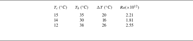
 Ra
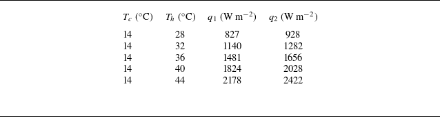
 q1
 q2
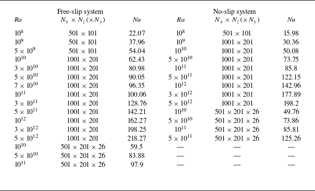
 Nx×Nz(×Ny)
 Nu

 U0
 σ
 x/l0=0.1
 x/l0=0.5
 Ra=109
 Ra=1010
 Ra=1011
 c1=1.85
 c2=1.2
 k1=3.63
 k2=1.63



 Nu
 Ra
 Pr=10
 Pr=0.1
 NuRa−1/4
 Ra
 Nu∼Ra1/5
 Nu∼Ra1/4
 Nu∼Ra1/5

 x/l0
 Ra=109

 U+≡U/uτ
 z+
 x/l0
 U+=z+
 U/U0
 ξ
 sech2[a1(ξ−ξp)]
 ξ⩾ξp
 a1
 ξp

 θ(ξ)
 ξ=z/λ
 0.1⩽x/l0⩽0.9
 Ra=5×10⁹
 5×10¹⁰
 5×1011
 x
 0⩽y/w0⩽1
 Ra=5×10¹¹
 a=0.63
 k1=5.48
 k2=2.46
 θdata−θfit
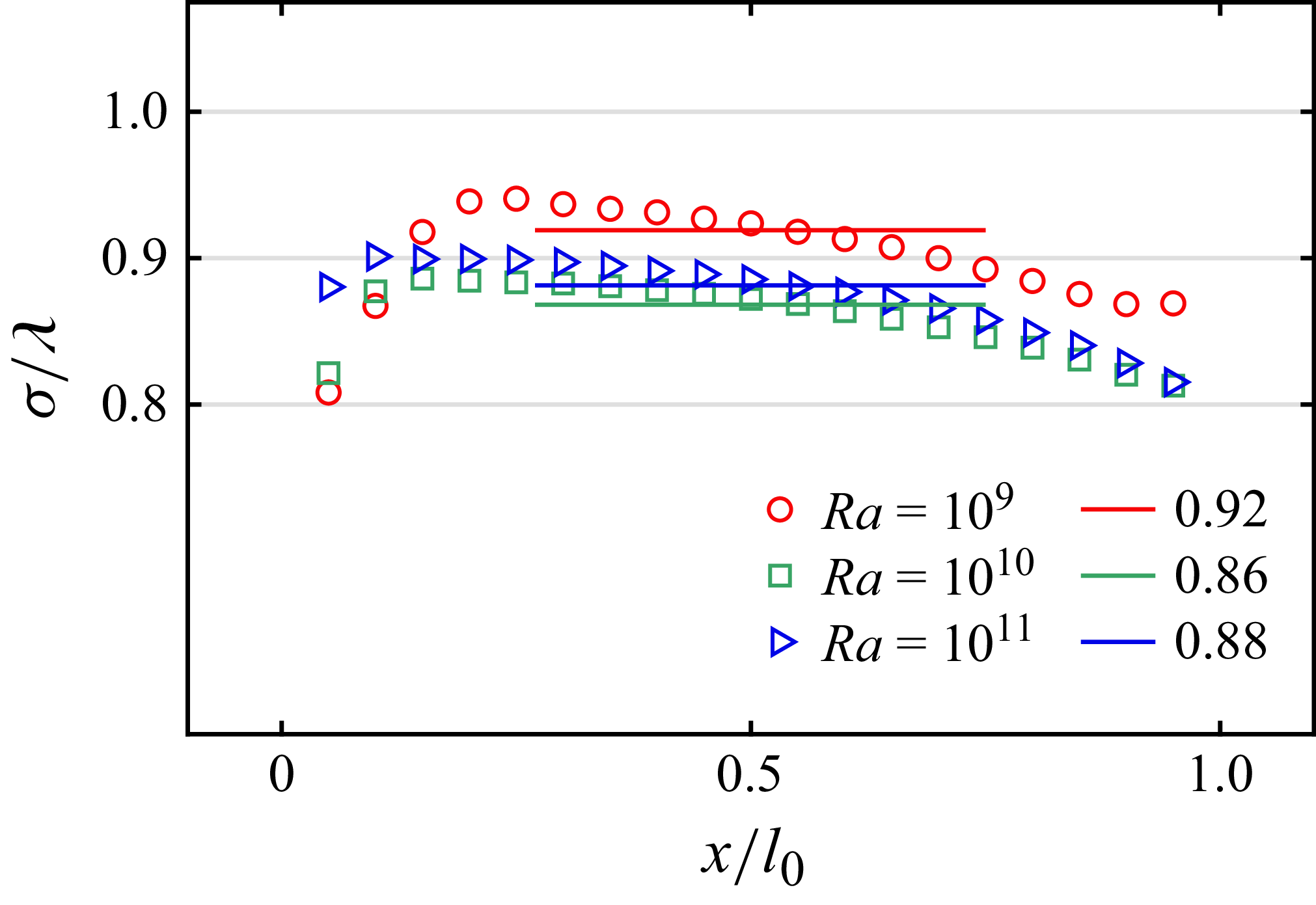
 σ
 λ

 Ra=109
 Ra=1011
 k1=3.57
 k2=1.6
 k1=3.79
 k2=1.7

 θ
 θdata−θfit
 Ra=1011
 H(ϵ,γ,δ,α,q)=H(−4.54,2.13,−0.13,−1.23,−0.61)
 c1=−0.91,c2=−0.002
 Ra=2.55×10¹²
 H(−4.13,2.03,−0.03,0.54,0.27)
 c1=−1.17,c2=0.002
 3⩽x/l0⩽7
 Ra=5×10⁹
 5×10¹⁰
 5×1011
 x
 0⩽y/w0⩽1
 Ra=5×10¹¹
 H(−2.81,1.70,0.30,−1.29,−0.64)
 c1=−1.06,c2=0.06
 H(−3.89,1.97,0.03,−0.06,−0.03)
 c1=−1.11,c2=0.02
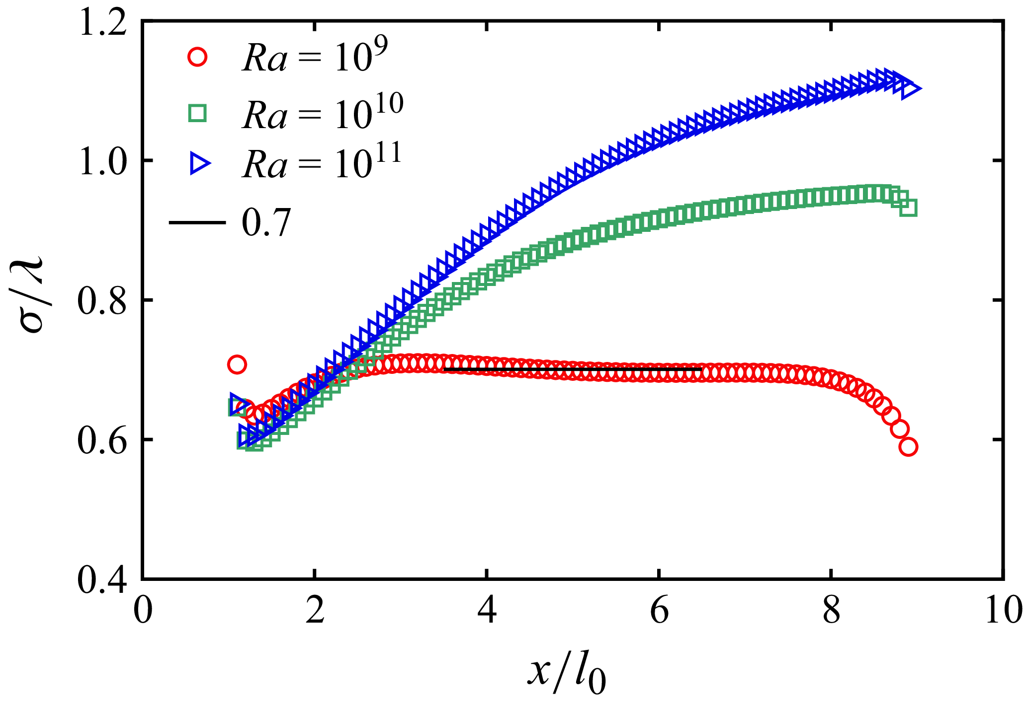
 σ
 λ=z0.7

 U0
 σ
 Ra=109
 Ra=1010
 k=0.82
 0.8

 θ(ξ)
 ξ=z/λ
 0.1⩽x/l0⩽0.9
 Ra=108
 109
 1010
 x
 0⩽y/w0⩽1
 Ra=1010
 k=2.6, c=−0.5
 k=3.61, c=−0.34
 k=6.36, c=−0.19
 θdata−θfit
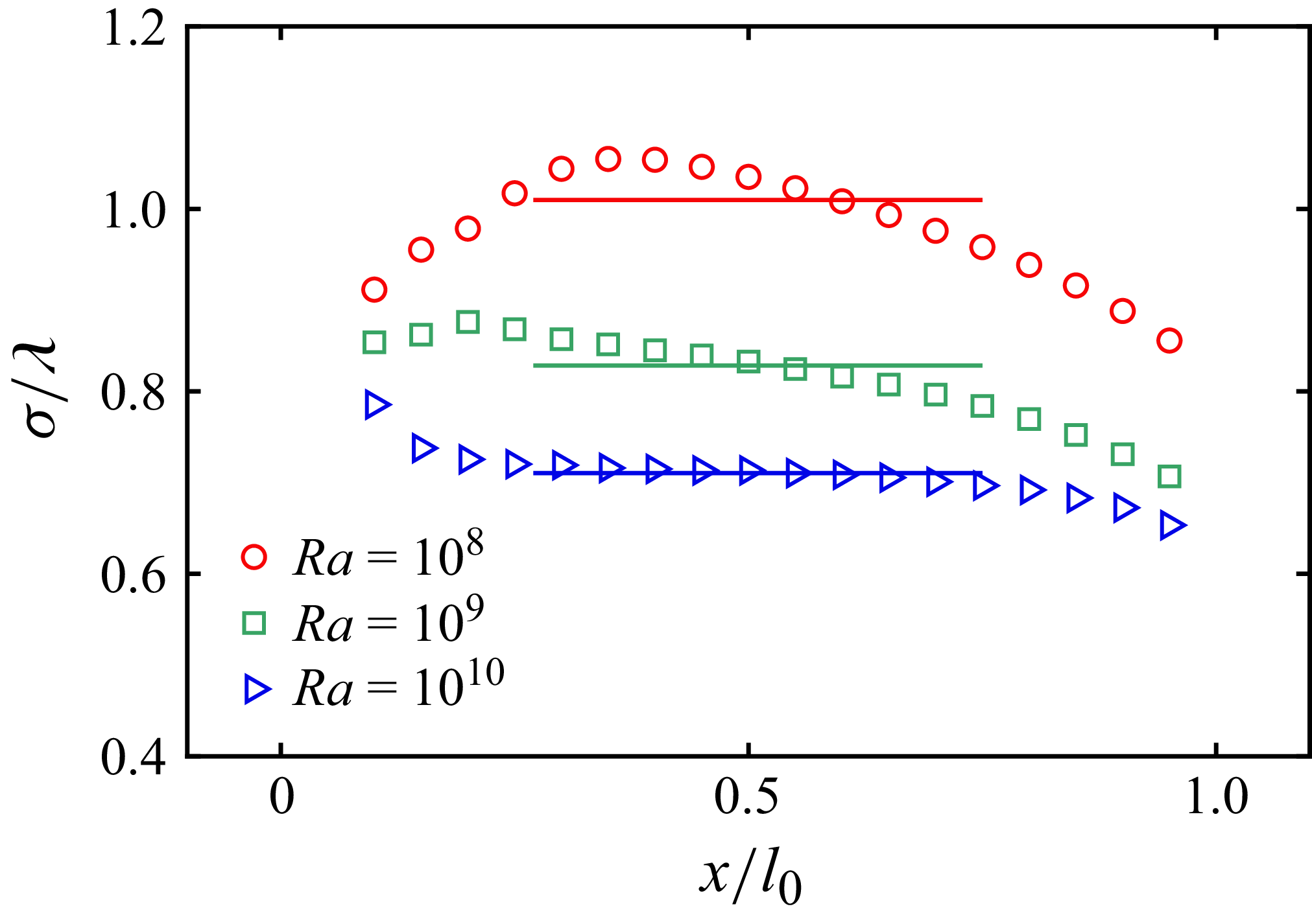
 σ
 λ

 x/l0
 Ra=109
 Ra=1010
 k=0.84
 k=0.85

 θ
 θdata−θ fit
 x/l0
 Ra=1010
 x/l0
 Ra=2.55×10¹²
 3≤x/l0≤7
 Ra=108
 109
 1010
 0≤y/w0≤1
 Ra=1010
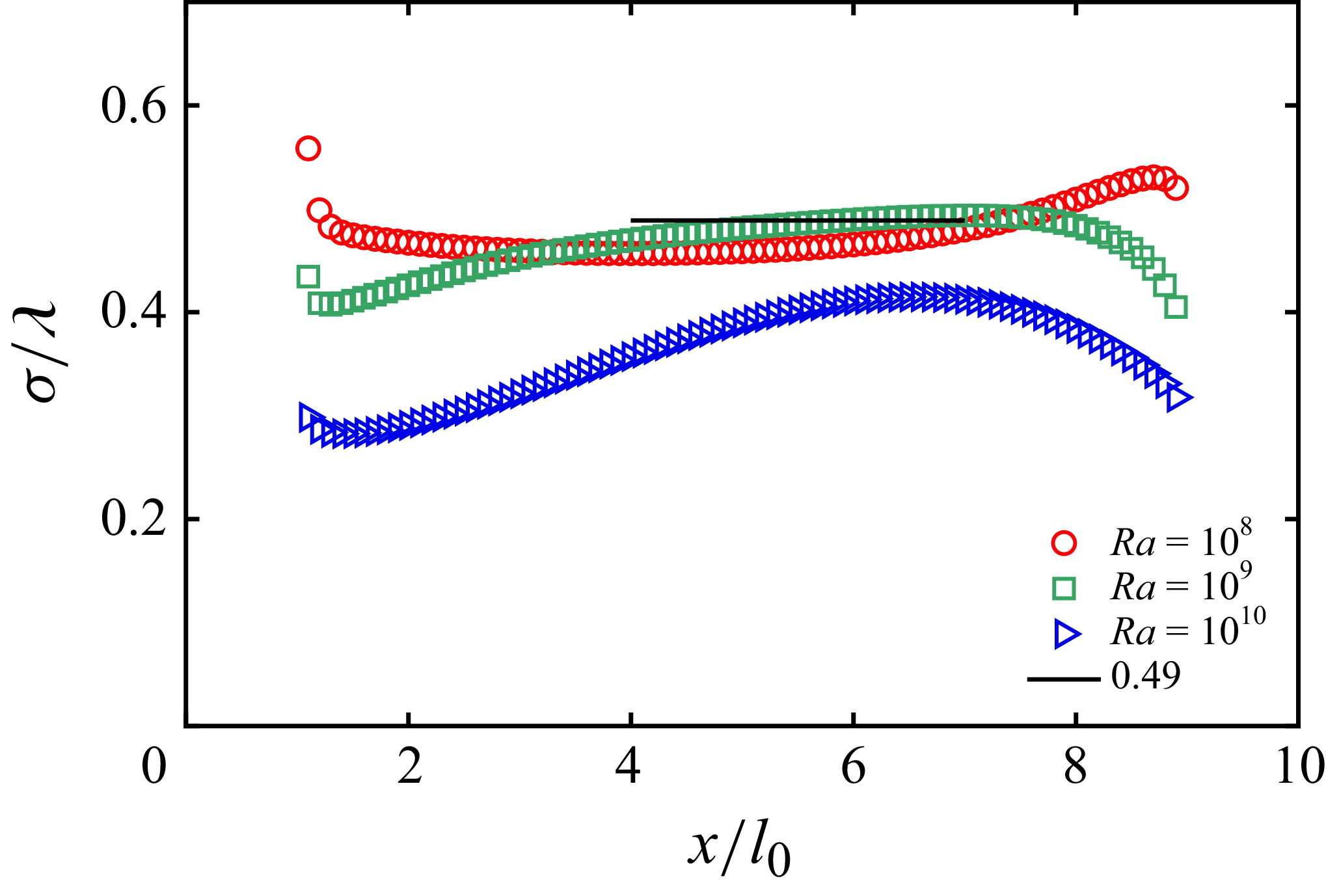
 σ
 λ=z0.7
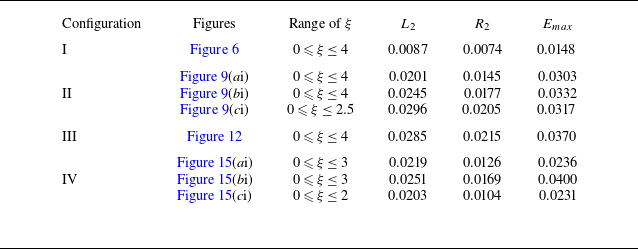
 L2
 R2
 Emax
 ξ
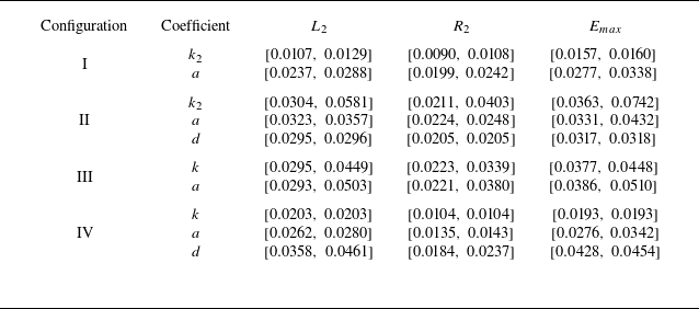
 ±5%
 L2
 R2
 Emax
 ±5%
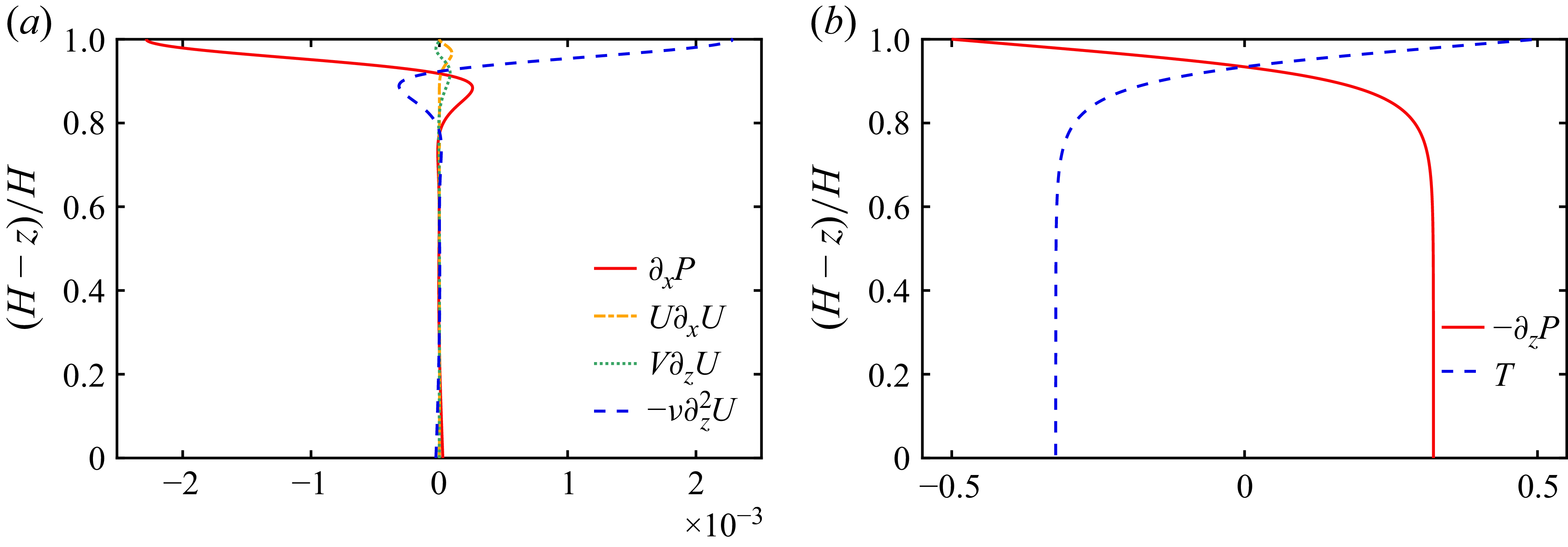
 ∂xP
 U∂xU,V∂zU
 −ν∂z2U
 −∂zP
 T
 0.1≤x/l0≤0.9
 Ra=1011

 U0=m1(x/l0)n1
 x/l0∈(0.1,1)
 n1=1.2
 Ra
 m1=0.02
 0.0135
 0.028
 Ra=109
 Ra=1011
 Ra=109
 x/l0∈(1,9)
 n1=0.25
 0.2
 0.18
 m1=0.0247
 0.0165
 0.04
 Px=m2(x/l0)n2
 Px
 x/l0∈(0.1,1)
 n2=1.15
 1.3
 1.95
 m2=0.009
 0.0045
 0.01
 x/l0∈(1,9)
 n2=−1
 −1.1
 −1.35
 m2=0.035
 0.0165
 0.025
 Re=m3(x/l0)n3
 x/l0∈(0.1,1)
 n3=1.1
 Ra
 m3=2
 5
 1.2
 x/l0∈(1,9)
 n3=0.5
 1.1
 0.8
 m3=2.9
 3.8
 1.5

 ΔTb(x)
 x/l0
 Ra
 a
 d
 Ra=1010
 1⩽x/l0⩽9
 0⩽x/l0⩽1
 9⩽x/l0⩽10

 Ra=1011
 F(α,β,γ)=F(0.5,−112.2,0.5)
 θ(ξ)=1.05ξ2
 θ(ξ)=1.9ξ3


