1 Introduction
Natural language sentences are built from complex interactions between content words (e.g., nouns, verbs) and function words (e.g., quantifiers, coordination). A well-founded, broad-coverage semantics should therefore jointly model lexical items and functional operators (Boleda and Herbelot Reference Boleda and Herbelot2016). Computational work on language and vision, however, has so far mostly focused on the lexicon, and representations of the general topic of text fragments. One strand of work in computer vision concentrates on content word representations, and nouns in particular (see, for example, Anderson et al. Reference Anderson, Bruni, Bordignon, Poesio and Baroni2013; Lazaridou, Pham and Baroni Reference Lazaridou, Pham and Baroni2015), whilst another is interested in approximate sentence representation, as in the Image Captioning and the Visual Question Answering shared tasks (VQA) (Hodosh, Young and Hockenmaier Reference Hodosh, Young and Hockenmaier2013; Antol et al. Reference Antol, Agrawal, Lu, Mitchell, Batra, Zitnick and Parikh2015; Xu et al. Reference Xu, Ba, Kiros, Cho, Courville, Salakhutdinov, Zemel and Bengio2015; Goyal et al. Reference Goyal, Khot, Summers-Stay, Batra and Parikh2016). Our work aims at filling the gap on the functional side of language, by exploring the performance of language and vision models on a particular logical phenomenon: quantification.
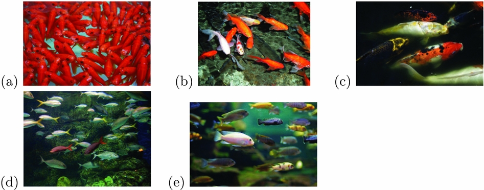
Quantification has been marginally studied in VQA, focusing on ‘number questions’ that can be answered with cardinals. It has been found that off-of-the-shelf state-of-the-art systems perform poorly on the type of questions (Ren et al. Reference Ren, Kiros and Zemel2015b; Antol et al. Reference Antol, Agrawal, Lu, Mitchell, Batra, Zitnick and Parikh2015) which require exact numerosity estimation, although recent work shows that it might be possible to adapt them to the counting task (Chattopadhyay et al. Reference Chattopadhyay, Vedantam, Selvaraju, Batra and Parikh2017). In this paper, we focus on a complementary phenomenon by considering quantifiers which involve (a) an approximate number estimation mechanism and (b) a quantification comparison step, i.e., the computation of a proportion between two sets. For instance, given the images in Figure 1, we want to quantify which proportion of fish are red fish. We define the task as a classification problem, involving the five classes (quantifiers) no, few, some, most and all. Our endeavour, as we argue below, is not simply an investigation of quantifiers. We claim that this specific problem is an interesting opportunity to reflect on the way we build neural network (NN) architectures.
Query: ____ fish are red. Answers: (a) All, (b) Most, (c) Some, (d) Few, (e) No.2

The research question: In linguistics, formal semanticists have extensively studied our expressions of interest under the broad topic of ‘generalised quantifiers’ (GQs; Barwise and Cooper, Reference Barwise and Cooper1981). The standard view – the one we are adopting in this paper – is that GQs are relations between a restrictor (e.g., fish), which selects a set of target objects in a state-of-affairs, and a scope (e.g., red) which selects the subset of the target set which satisfies a certain property. These two components determine their logical structure. Alternatively, they can be seen as imposing a condition on the proportion between the selected sets, e.g., |redfish|/|fish|.
This proportional property of GQs necessitates an operation at a level of abstraction which, we think, is interestingly different from the level of shallow reasoning needed to process content words and simple cardinals. The intuition behind our conjecture can be explained by considering the following. Let us assume that we want to find the correct quantifier for a particular concept-feature pair (e.g., fish–red), given a specific image (see Figure 1, where the task is to return which proportion of fish are red). We want the network to learn that certain quantifiers correspond to certain set configurations: given sets A and B, if A∩B is nearly entirely contained in A, then it is true that most As are Bs; if the overlap is less, then few or some As are Bs. There is a correlation to be learnt between different set configurations and particular quantifiers, but those configurations are abstractions over the raw linguistic and visual data: when the set comparison takes place, it is irrelevant whether As are fish or ice cream scoops, or indeed, how many As exactly were observed. A language and vision system faced with the task to quantify thus has to generalise beyond the standard tasks if identifying and naming objects or properties in an image. Whilst these steps are required, they are only the fundament of a more complex process by which the system must abstract over the identified entities to perform well. Our question in this work is ‘can this process of abstraction be modelled by an NN architecture?’
One likely hurdle for current state-of-the-art systems is the need to keep away from category-level statistics which can be so informative in many language and vision tasks. With quantifiers, attempting to use category-level information (e.g., generally speaking, twenty per cent of all fish are red) will result in failure to generalise to randomly sampled subsets of small cardinality. Figure 1 illustrates the point, where knowledge of fish or redness is not enough for the predictive power of the system.Footnote 1 Similarly, the amount of overlap between two sets can be associated with particular quantifiers regardless of the cardinality of those two sets, what matter is their proportion. So an ideal model will learn to abstract over cardinality information too.
The strategy we propose to learn to quantify is to divide the task into two subtasks: (a) learn an abstract, category-free representation of the raw data and (b) learn quantification over the abstract representation. The high results obtained in Sorodoc et al. (Reference Sorodoc, Lazaridou, Pezzelle and Bernardi2016), who have trained NNs to quantify over synthetic scenarios of coloured dots, suggest that NNs should be able to learn the second subtask quite easily. In this paper, we study how far current strategies to integrate the language and vision modalities are suitable when put to work on the full task, involving quantification over real-life images. We revisit some state-of-the-art VQA models, considering some of the NN features which may affect how the model deals with this high-level process. In particular, we focus on (a) the role of sequential processing of the data in both language and vision modalities and (b) so-called ‘attention’ mechanisms, within and across modalities, viz., the ability of the system to ‘focus’ on the right part of the data at the right time in processing.
Assumptions: It should be mentioned that the connection between quantifiers and numbers (or proportions), though apparently trivial, is largely debated. The positions range from claiming that quantifiers can be mapped to an ordered numerical scale (Bass et al. Reference Bass, Cascio and O’connor1974; Holyoak and Glass Reference Holyoak and Glass1978; Hammerton Reference Hammerton1976), to proposing that the meaning of these expressions is dependent on many factors and might even not convey any quantitative information (Moxey and Sanford Reference Moxey and Sanford1993; Nouwen Reference Nouwen2010). The present work does however not engage with those debates, and stays clearly in the GQ tradition. Further, we make the following simplifying assumptions regarding formalisation of quantifiers. First, we give each one of our quantifiers a fixed interpretation (e.g., most corresponds to a ratio of at least seventy per cent of the restrictor satisfying the condition of the scope), and we assume the quantifiers do not overlap. That is, in our setting, there is one ‘correct’ quantifier per instance scenario. Second, we do not engage with pragmatic questions relating to use of quantifiers, such as inter-speaker variations and context dependence. We believe these simplifications make our evaluation more tractable and do not affect our architectural claims.
Contributions: We make two main contributions in this paper. First, we identify elements that are crucial to the good functioning of a neural quantificational architecture. We show that, as in the case of content words, attention mechanisms help to obtain a more salient representation of the linguistic and visual input, useful for the processing of quantifiers. In particular, they suitably estimate the approximate number of the two sets involved in the quantification operation. We also show that a network informed by linguistic theory, which reproduces the logical structure of GQs, works better than less structured architectures. Second, we propose a new quantification dataset (Section 3), informed by the current debate of balancing datasets of natural images. This debate was started by Zhou et al. (Reference Zhou, Tian, Suhkbaatar, Szlam and Fergus2015), who demonstrated that a simple bag-of-word (BOW) baseline, that concatenates visual and textual inputs, can achieve very decent overall performance on the VQA task. This prompted ideas that the high results obtained by language and vision systems on the VQA dataset might be due to a language bias (Zhang et al. Reference Zhang, Goyal, Summers-Stay, Batra and Parikh2016; Johnson et al. Reference Johnson, Hariharan, van~der~Maaten, Fei-Fei, Zitnick and Girshick2017). This issue has subsequently been addressed in datasets using, e.g., synthetic scenes or similar natural images corresponding to different answers (Goyal et al. Reference Goyal, Khot, Summers-Stay, Batra and Parikh2016). Our dataset follows this line of work, making sure that the entity sets that the system is required to quantify over do not exhibit unwanted regularities.
2 Related work
2.1 Computational and psycholinguistic models of quantifiers
The problem of algorithmically describing logical quantifiers was first addressed by van Benthem (Reference van Benthem1986) using automata. Following these first efforts, a lot of work has been done in computational formal semantics to model quantifiers in language (see, e.g., Szabolsci, Reference Szabolsci2010; Keenan and Paperno, Reference Keenan and Paperno2012 for an overview). Recently, distributional semantics has turned to the problem, with Baroni et al. (Reference Baroni, Bernardi, Do and Shan2012) demonstrating that some entailment relations hold between quantifier vectors obtained from large corpora, and Herbelot and Vecchi (Reference Herbelot and Vecchi2015) mapping a distributional vector space to a formal space from which the quantification of a concept–property pair can be predicted. This line of work, however, only considers the linguistic modality, without paying attention to the visual one.
In parallel to the formal linguistic models, psycholinguistics has studied function words from a statistical perspective using NN architectures. At the end of the 90s, Dehaene and Changeux (Reference Dehaene and Changeux1993) showed how approximate numerosity could be extracted from visual input without serial counting, bringing computational evidence to the psycholinguistic observation that infants develop numerosity abilities before being able to count (Xu and Spelke Reference Xu and Spelke2000; McCrink and Wynn Reference McCrink and Wynn2004). This is also in line with evidence showing that this ability, in children, is not required for the comprehension and production of quantifiers (Hurewitz et al. Reference Hurewitz, Papafragou, Gleitman and Gelman2006; Halberda, Taing and Lidz Reference Halberda, Taing and Lidz2008).
Of particular interest to us, Rajapakse et al. (Reference Rajapakse, Cangelosi, Conventry, Newstead and Bacon2005) aimed at computationally grounding linguistic quantifiers in perception. The quantifiers studied were a few, few, several, many and lots, and the system was trained on human annotations of images consisting of stripy (target) and white (non-target) fish. Given an image, the model had to predict which number of fish was stripy, using the given quantifiers. The authors showed that both the number of targets (stripy fish) and their spacing played a role in the prediction, though the model neither used information regarding the number of non-targets (white fish) nor spatial grouping, in contrast with behavioural evidence (Coventry et al. Reference Coventry, Cangelosi, Newstead, Bacon and Rajapakse2005, Reference Coventry, Cangelosi, Newstead and Bugmann2010).
The above-mentioned computational studies were touching upon an interesting research avenue, but the NN architectures available at the time (particularly on the visual side) were not advanced enough for a thorough investigation. In the meantime, interesting progress on modelling the acquisition of quantifiers in a Bayesian probabilistic framework has been reported (Piantadosi, Tenenbaum and Goodman Reference Piantadosi, Tenenbaum and Goodman2012; Piantadosi Reference Piantadosi2011). More recently, NNs have been shown to perform well in tasks related to quantification, from counting to simulating the approximate number sense (ANS). Seguí, Pujol and Vitria (Reference Seguí, Pujol and Vitria2015), for instance, explore the task of counting occurrences of an object in an image using convolutional neural networks (CNNs), and demonstrate that object identification can be learnt as a surrogate of counting. Stoianov and Zorzi (Reference Stoianov and Zorzi2012) show that the ANS emerges as a statistical property of images in deep hierarchical generative models. Very interesting models have also been proposed by Chattopadhyay et al. (Reference Chattopadhyay, Vedantam, Selvaraju, Batra and Parikh2017), who focus on the issue of counting everyday objects in visual scenes. In doing so, they adopt strategies inspired by ‘subitising’, an ability which is almost universally shared in the animal domain and allows humans to rapidly and automatically represent discrete quantities up to three or four items. Similarly, focusing on the subitising mechanism, Zhang et al. (Reference Zhang, Ma, Sameki, Sclaroff, Betke, Lin, Shen, Price and ech2015) address the issue of salient object detection and show how CNN models can discriminate between images with 0 to 4+ salient objects. As discussed by Borji et al. (Reference Borji, Cheng, Jiang and Li2015), the salient object detection task highly depends on various properties of the images, like the uniformity of the various regions, the complexity of the foreground and background, how close to each other the salient objects are and how they differ in size.
The models we present in this paper can be seen as a continuation of previous work on linguistic quantifiers. As in Dehaene and Changeux (Reference Dehaene and Changeux1993), the systems we evaluate do not rely on explicit counting, and use the gist of the objects in an image to produce the appropriate quantifier for a given scenario. We also follow Rajapakse et al. (Reference Rajapakse, Cangelosi, Conventry, Newstead and Bacon2005) in their investigation of ‘vague’ linguistic quantifiers, but we train and evaluate our system on real images rather than toy examples. Unlike them, however, we do not investigate object position in the image and start from their bounding boxes (BBs).
To our knowledge, Sorodoc et al. (Reference Sorodoc, Lazaridou, Pezzelle and Bernardi2016) and Pezzelle, Marelli and Bernardi (Reference Pezzelle, Marelli and Bernardi2017) are the only recent attempt to model non-cardinals in a visual quantification task, using NNs. Pezzelle, Marelli and Bernardi (Reference Pezzelle, Marelli and Bernardi2017) focus on the difference between the acquisition of cardinals and quantifiers, showing they can be modelled by two different operations within the network, and learning one function per cardinal/quantifier. Our paper can be seen as extending the work of Sorodoc et al. (Reference Sorodoc, Lazaridou, Pezzelle and Bernardi2016) by (a) augmenting their list of logical quantifiers (no, some, all) with proportional ones (few, most); (b) moving from artificial scenarios with geometric figures to real images; (c) most importantly, treating quantifiers as relations between two sets of objects amongst a number of distractors (in contrast, their scenarios only include objects of the same type, e.g., circles, and the task is to quantify over the colour property of those circles).
2.2 Datasets with numerosity annotation
COCO-QA (Ren, Kiros and Zemel Reference Ren, Kiros and Zemel2015a) was the first dataset of images associated with number questions. COCO-QA consists of around 123 K images extracted from Lin et al. (Reference Lin, Maire, Belongie, Hays, Perona, Ramanan, Dollar and Zitnick2014b), and 118 K questions generated automatically from image descriptions. Number questions are one of the four question categories (together with object, colour and location) and make up 7.47 per cent of the overall questions both in the training and test datasets. For this category, the authors observe that the evaluated models can sometimes count up to 5 or 6. However, this ability is fairly weak as they do not count correctly when presented with unknown object types. Starting from Lin et al. (Reference Lin, Maire, Belongie, Hays, Perona, Ramanan, Dollar and Zitnick2014b) and Antol et al. (Reference Antol, Agrawal, Lu, Mitchell, Batra, Zitnick and Parikh2015) built the VQA dataset, aiming to increase the diversity of knowledge and kinds of reasoning needed to provide correct answers. VQA consists of around 200 K images, 614 K questions and 6 M ground truth answers. It contains open-ended, free-form questions and answers provided by humans. The evaluation of state-of-the-art models against this dataset confirmed that number questions are hard to answer and require good combined understanding of the language and vision modalities. The difficulty of number questions was further highlighted in Johnson et al. (Reference Johnson, Hariharan, van~der~Maaten, Fei-Fei, Zitnick and Girshick2017), where the authors introduced Compositional Language and Elementary Visual Reasoning diagnostics, a dataset allowing for an in-depth evaluation of current VQA models on various visual reasoning tasks. The reasoning skills they investigated (querying object attributes, counting sets of objects or comparing values, existence questions) are close to the task we propose. They show that state-of-the-art systems perform poorly in situations requiring short-term memory (attribute comparison and integer equality).
Focusing on the subitising phenomenon, the Salient Object Subitising dataset, proposed in Zhang et al. (Reference Zhang, Ma, Sameki, Sclaroff, Betke, Lin, Shen, Price and ech2015), contains about 14 K everyday images annotated with respect to numerosity of salient objects (from 0 to 4+). Images were gathered from various sources (viz. COCO, ImageNet, VOC07 and SUN) and filtered out to create a balanced distribution of images containing obviously salient objects. To eliminate the bias due to unbalanced number distribution (indeed, most of the images contained 0 or 1 salient objects), the authors generated and used synthetic Salient Object Subitising image data.
None of the datasets above meet our needs for the quantification task. In Salient Object Subitising images, salient objects are all of the same category and properties are not annotated. Only small numerosities are represented. As for VQA, it does contain annotated objects of different categories but does not provide annotation of properties. Very recently, however, a new version of COCO-QA, COCO Attribute-QA, has been released. It contains images annotated with both objects (of various categories) and properties (Patterson and Hays Reference Patterson and Hays2016). It consists of 84 K images, 180 K unique objects (from twenty-nine object categories) and 196 attributes, for a total of 3.5 M object–attribute pairs. We take this as our starting point to create a dataset of natural images which can be matched to the range of quantifiers in our study (see Section 3).
2.3 Neural networks for VQA
Since the pioneer work by Malinowski and Fritz (Reference Malinowski and Fritz2014) and Geman et al. (Reference Geman, GErman, Hallonquist and Younes2015), many researchers have taken up the VQA challenge. Most of them have based their system on NN models (Gao et al. Reference Gao, Mao, Zhou, Huang and Yuille2015; Ren et al. Reference Ren, Kiros and Zemel2015b; Malinowski, Rohrbach and Fritz Reference Malinowski, Rohrbach and Fritz2015; Ma, Lu and Li Reference Ma, Lu and Li2016) that can learn to perform the given task in an end-to-end fashion. The first NNs proposed to tackle VQA were based on a combination of global visual feature vectors extracted by a CNN, and text feature vectors extracted using a long Short-term memory network (LSTM). Various LSTM–CNN models have been proposed which differ with regard to the way these two types of features are combined (multimodal pooling): by mere concatenation (Zhou et al. Reference Zhou, Tian, Suhkbaatar, Szlam and Fergus2015), or by more complex operations like element-wise multiplication (Antol et al. Reference Antol, Agrawal, Lu, Mitchell, Batra, Zitnick and Parikh2015) or multimodal compact bilinear pooling (Fukui et al. Reference Fukui, Park, Yang, Rohrbach, Darrell and Rohrbach2016). Proposals have also been made to use solely one type of network (CNN or LSTM). Ren et al. (Reference Ren, Kiros and Zemel2015a) use an LSTM to jointly model the image and the question: they treat the image as a word appended to the question, and the image is processed by a CNN model, the output of which is frozen during the training process. More recently, on the opposite site, a convolutional architecture has been used to learn both types of feature and their interaction (Ma et al. Reference Ma, Lu and Li2016).
Significant progress has been made on the VQA task by introducing memory and attention components, taken from other areas of language and vision. Xu et al. (Reference Xu, Ba, Kiros, Cho, Courville, Salakhutdinov, Zemel and Bengio2015), for instance, introduced an attention-based framework into the problem of image caption generation. Memory networks have been used to tackle tasks involving reasoning on natural language text (Weston, Chopra and Bordes Reference Weston, Chopra and Bordes2015; Sukhbaatar et al. Reference Sukhbaatar, Szlam, Weston and Fergus2015). A combination of both the memory and attention components have been proposed by, e.g., Kumar et al. (Reference Kumar, Irsoy, Su, Bradbury, E, Pierce, Ondruska, Gulrajani and Socher2016) and recently applied to the VQA challenge in the Dynamic Memory Network (DNM+; Xiong, Merity and Socher Reference Xiong, Merity and Socher2016) and Stacked Attention Networks (SANs; Yang et al. Reference Yang, He, Gao, Deng and Smola2016). Andreas et al. (Reference Andreas, Rohrbach, Darrell and Klein2016a, Reference Andreas, Rohrbach, Darrell and Klein2016b) further combine the dynamic properties of previous models with the compositionality process of natural language questions via reinforcement learning.
We build on this previous work by porting insights from the VQA task to our quantification task. In particular, we investigate the role of LSTMs and their combination with CNNs, both as simple concatenation and within stacked attention mechanisms. In the end, we propose a model that combines formal semantics intuitions about quantifiers (as relations between a restrictor and a scope), and the latest findings of VQA models on attention mechanisms.
3 Data
For our task, the required datapoints are in the form 〈scenario, query, answer〉. The answer is a quantifier among five possible ones (no, few, some, most or all). The query is an 〈object, property〉 pair (e.g., 〈 dog, black 〉) such that the object and the property correspond to the restrictor and scope of the quantifier, respectively. The scenario is an image containing objects which may or may not be of the type of the restrictor, and may or may not have the property expressed by the scope. We will refer to the objects that have the required property (e.g., black dogs) as target objects.
We take quantifiers to stand for fixed relations (operationalised as proportions) between the relevant sets of objects:  $\frac{|\text{restrictor} \cap \text{scope}|}{|\text{restrictor}|}$. Hence, we take no and all to be the correct answer for scenarios in which the target objects are zero per cent and hundred per cent of the restrictor set, respectively. To define few and most, we use prevalence estimates reported by Khemlani Leslie and Glucksberg for low-prevalence and majority predications. In particular, we assign few to ratios lower than or equal to seventeenpercent, and most to ratios equal to or greater than seventy per cent. All ratios ranging between these two values are assigned to some.
3.1 From COCO ATTRIBUTE to Q-COCO
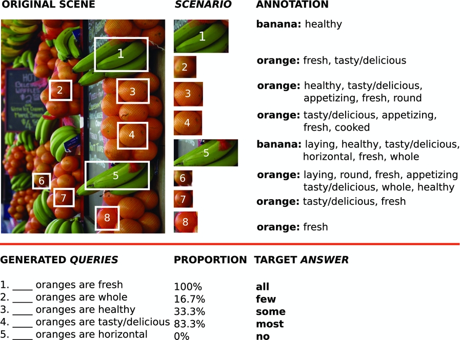
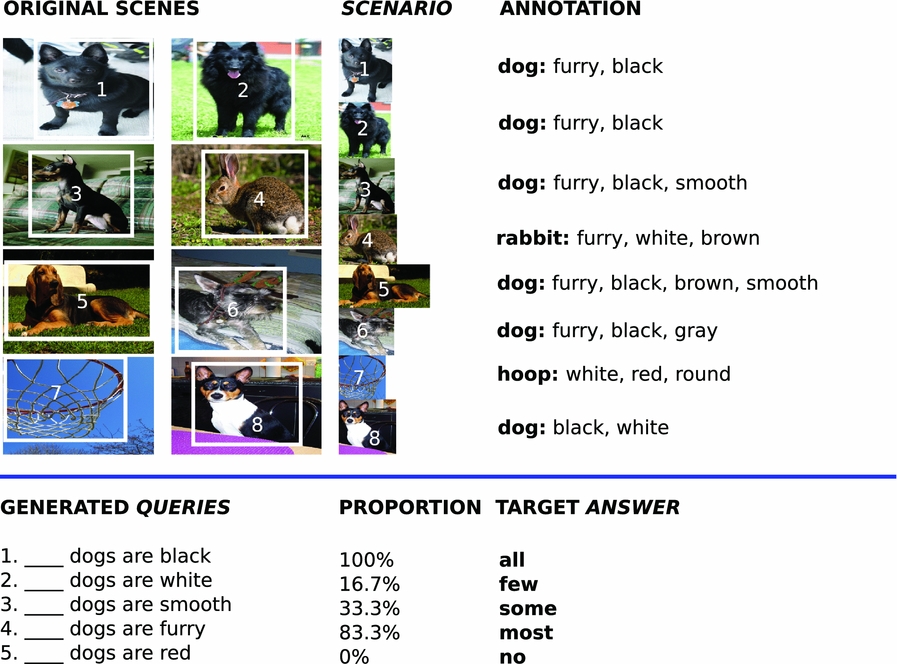
COCO-Attribute (Patterson and Hays Reference Patterson and Hays2016) is a dataset with comprehensive property annotation. It contains 84 K image from MS-COCO (Lin et al. Reference Lin, Maire, Belongie, Hays, Perona, Ramanan, Dollar and Zitnick2014a). Some of the objects are marked with region coordinates/BBs, and their properties (‘attributes’ in COCO terminology) have been annotated by humans. In total, there are twenty-nine object categories (types of objects), 196 properties and 180 K annotated regions, with an average of nineteen properties per annotated object. Not all objects in an image are annotated with respect to properties: only objects in the twenty-nine object categories, and for which BBs are provided, are annotated. Hence, we cannot exploit the full image, but must restrict ourselves to the annotated regions. As illustrated in Figure 2, we construct Q-COCO scenarios from this data, following the procedure described below.
Generation of datapoints in the form of triplets <query, scenario, answer> for the Q-COCO dataset.

First of all, we filter out all images containing less than six annotated objects, thus obtaining 5,203 unique images. This choice is motivated by the fact that six is the lowest restrictor cardinality that allows us to have all five quantifiers represented in the data, given the ratios we have assigned to them. To clarify this point, zero out of six objects would be a case of no; one out of six would be few; two, three and four would be some; five would be most and six would be all. Note that if we had used five objects instead of six, few would not have been represented. So this constraint is a necessary (though not sufficient) condition to avoid bias due to restrictor cardinality.
Second, for each of these 5,203 images, all properties associated with each annotated object are extracted. We compute the overall frequency of each property and, to avoid data sparsity, we retain only properties with frequency >1, 000. That is, if the object ‘banana’ in a given image is originally annotated with three properties (e.g., appetizing, fresh, delicious), only the most frequent ones are included (e.g., appetizing, fresh). This way, we obtain forty-four unique properties. Finally, we retain only the images containing at least six annotated objects that belong to the same category (e.g., banana).
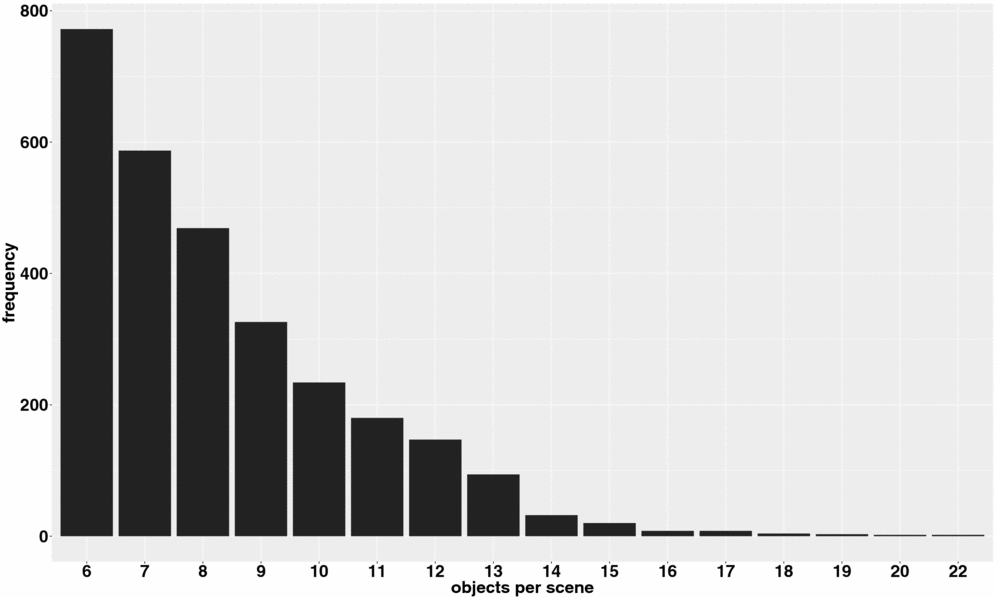
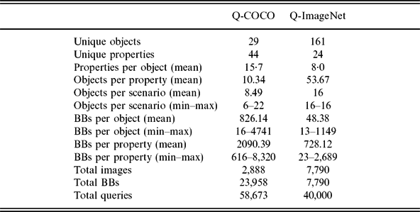
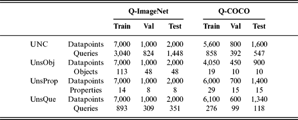
As reported in Table 1, the resulting dataset includes 2,888 unique images depicting 23,958 annotated objects. On average, each image contains 8.49 annotated objects, each of which has on average eight properties. As mentioned above, the scenarios of Q-COCO consist of the BBs extracted from these images and their object–property annotations. Figure 3 reports the distribution of scenarios with respect to the number of annotated objects included. As can be seen, scenarios containing up to ten objects are the vast majority (around eighty-three per cent of the total).
Distribution of Q-COCO images against number of annotated objects. Number of annotated objects (X-axis) ranges from 6 to 22.

Descriptive statistics for Q-COCO and Q-ImageNet datasets

Using these annotations, for each of the 2,888 unique scenarios, we generate all possible queries and corresponding quantifier following the ratios defined above. To avoid including implausible queries such as ‘metallic banana’, when generating queries whose answer is no, we ensure that only properties which occur together with the target object in at least one annotation are included. Figure 2 shows some of the queries generated from the annotation of one real image included in our dataset.
In total, 58,673 queries are generated (mean: 20.32 queries per image). Out of all 58,673 queries, the most represented quantifier turns out to be no (31,222 cases), followed by some (13,313), few (9,009), most (3,501) and all (1,628). We balance their distribution when creating the various experimental settings against which we evaluate the models (see Section 4 for more detail).
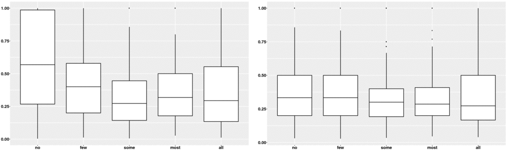
It is evident from the literature (see Section 2) that datasets of natural images can be biased towards the linguistic modality. To check whether this applies to Q-COCO, we analyse a sample of its datapoints by randomly selecting a balanced number of cases for each quantifier. For each query (e.g., ‘black, dog’), we compute the number of times it occurs paired with a given quantifier, e.g., ‘black, dog, all’, in the sample dataset. We then divide this frequency by the total number of times the query ‘black, dog’ appears in the sample dataset. This way, we obtain a ratio describing the bias of each query towards each quantifier. If ‘black, dog’ appears ten times in the dataset, and these ten cases are equally split among the five quantifiers (two cases for ‘no’, two cases for ‘few’ and so on), then the dataset can be considered as perfectly balanced, having around twenty per cent of cases per each quantifier. If most cases correspond to one or few specific quantifiers, then the dataset is biased. In Figure 4 (left), we plot the distribution of these ratios relative to each quantifier.
Distributions of datapoints with respect to their frequency with a given quantifier in Q-COCO (left) and Q-ImageNet (right).

As can be seen, no and few are particularly biased, meaning that a model could simply learn correlations between object–properties and quantifiers in order to give the right answer when tested with a seen query. This limitation of the dataset cannot be easily solved, since any real-image dataset is likely to contain correlations that depend on object–property relations. To illustrate, ‘banana, metallic’ – if present – is likely to appear with the quantifier no (and perhaps few), but not with most and all. This finding illustrates a general issue, since carrying out quantification tasks using real images might always be affected by such regularities between object–property distributions in the real world. But, as we argued in the introduction, quantifiers per se are logical functions that can in principle apply to sets of any composition.
Given the inherent bias in the object distribution of real images, we also investigate the use of a synthetic dataset built from real images. To do this, we select ImageNet as visual corpus, since it contains more object categories and all annotated properties are visual (compare with COCO-Attribute, where properties are not necessarily visual: see Figure 2).
3.2 From imagenet to Q-imagenet
ImageNet (Deng et al. Reference Deng, Dong, Socher, Li, Li and Fei-Fei2009) contains 1,073,739 images annotated with BBs. Out of 3,000 object categories (‘synsets’ in ImageNet terminology), 375 are also provided with human annotations of properties, representing a total of twenty-five unique attributes. ImageNet images are rather different from those in COCO Attribute: most of the time, they do not contain multiple objects.
As in Q-COCO, we create Q-ImageNet scenarios from the BBs in the image. But only one BB is extracted from each image. As a result, the dataset differs from Q-COCO in that it merges together BBs that do not originally belong to the same image, giving us more leeway to overcome the bias found in real scenes.
We build synthetic scenarios that are made up of sixteen different BBs. This choice is motivated by two considerations. First, in Q-COCO, ninety-nine per cent of images contain sixteen or fewer objects and so sixteen can be considered as a reasonable ‘realistic’ upper bound. Second, this number allows us to have a fairly large variability with respect to the cardinalities of both restrictor and scope.
We use the 375 objects associated with the twenty-five annotated property labels, and the corresponding images. We then select all ImageNet items annotated with at least one of those properties and extract the BB for which the human annotation has been performed. This results in 9,597 BBs. This set is subsequently filtered according to the criterion that the property words must occur at least 150 times in the UkWaC corpus (Baroni et al. Reference Baroni, Bernardini, Ferraresi and Zanchetta2009): this ensures the quality of the corresponding word embeddings. As reported in Table 1, after this filtering process, we end up with 161 different objects associated with 7,790 BBs, and labelled with twenty-four properties. On average, each object has 48.38 unique BBs, it is assigned eight properties and each property is shared by 53.67 objects.
As in Q-COCO, we use our set of objects–properties to construct 〈scenario, query, answer〉 datapoints. In this case, we generate a query by randomly choosing the label l of one of the 161 objects and a property p out of the twenty-four properties. In doing so, we follow the same plausibility constraint used for the previous dataset, in that we only use 〈object, property〉 pairs that occur together at least once in the annotated images. We then assign one quantifier to each scenario-query combination. Further, to make our synthetic scenarios as plausible as possible, we also set a constraint on the distractor images in each datapoint. We use an association measure based on MS-COCO captions (Lin et al. Reference Lin, Maire, Belongie, Hays, Perona, Ramanan, Dollar and Zitnick2014b), which evaluates the chance of two objects to appear together in a real image. The idea is that objects that are more likely to occur together make more realistic scenarios and should thus be preferred in the generation process (for instance, a dog and a sofa are more often seen together than a sofa and an elephant). We compute Pointwise Mutual Information (PMI) as a proxy for the likelihood of two objects to co-occur in an image:
 \begin{equation}
\text{PMI}(o1, o2) = \text{log}\frac{f(o1, o2) * N}{f(o1) * f(o2)}
\end{equation}
where o1 and o2 are two objects, f(o1, o2) is the number of times words o1 and o2 co-occur in a single caption, f(o) is o’s frequency in the captions of MS-COCO overall and N is the number of words in all captions. If an object’s label does not occur in the captions, it is considered to have the same probability of co-occurrence with all other objects.Footnote 3 When selecting distractors for the object of interest in a particular scenario, we randomly pick them based on their likelihood of co-occurrence with that object. Technically, a probability distribution is computed based on the PMI score to assign high probability values to high-PMI pairs, low probability values to low-PMI ones. This way, the chance to select a distractor that frequently co-occurs with the target object is maximised.
We check whether Q-ImageNet has a language bias by applying the same method used for Q-COCO. In Figure 4 (right), we plot the distribution of the datapoints against the proportion of cases a given query does occur with a given quantifier. As above, the proportion is computed by dividing the number of occurrences of a query with a given quantifier (e.g., ‘black, dog, all’) by the total number of cases of that query (e.g., ‘black, dog’). As can be noticed, the distribution is much better compared to the real-image dataset (Q-ImageNet). On average, our datapoints are around or slightly over chance level (twenty per cent), indicating that there is an almost equal number of cases for each quantifier to occur with a given query. Figure 5 shows an example of a scenario in Q-ImageNet, together with the associated queries and corresponding gold answers.
Generation of datapoints in the form of triplets <query, scenario, answer> for the Q-ImageNet dataset. Note that, for sake of clarity, we represent the scenario as made up by eight images instead of sixteen.

4 Experimental settings
For both datasets, we experiment with four experimental settings which let us test the behaviour of the system under different training conditions.
Uncontrolled (UNC): From the whole set of generated datapoints, we randomly select a balanced number of cases for each quantifier. In this setting, it is possible to encounter known scenarios or queries at test time, but scenario-query combinations are all unseen. (This setting is basically the sampled data used to control dataset bias in the previous section.)
Unseen objects (UnsObj): This setting tests the generalisation power of our models over scenarios containing unseen objects. We randomly divide our list of concepts and pick seventy per cent for training, thirty per cent for testing/validation. For each concept, we then randomly select a balanced number of differently quantified datapoints.
Unseen properties (UnsProp): Similarly to UnsObj, this setting tests the generalisation power of our models with respect to properties. The procedure followed to obtain the dataset used in this setting is the same as for the UnsObj setting, except that we split the datapoints according to the properties.
Unseen queries (UnsQue): The last setting tests generalisation with respect to unseen combinations 〈object, property〉. For instance, the system sees both dog and black in training, but 〈dog, black〉 only at test time. To build this setting, we first randomly select seventy per cent 〈object, property〉 tuples for training and thirty per cent tuples for testing and validation. We then follow the same procedure as above.
Details of the composition of the training, validation and test sets are given in Table 2.
Q-ImageNet and Q-COCO training, validation and test sets of the three experimental settings

5 Models
We experiment with seven different models, to compare the contribution of various mechanisms and architectures in the quantification task. The first two models, ‘blind’ BOW and BOW+CNN, are simple baselines from the VQA literature adapted from Zhou et al. (Reference Zhou, Tian, Suhkbaatar, Szlam and Fergus2015). They show how a language-only model performs over one-hot representations, and over a simple concatenation of one-hot language vectors and CNN image representations. The next two models, ‘blind’ LSTM and LSTM+CNN (Antol et al. Reference Antol, Agrawal, Lu, Mitchell, Batra, Zitnick and Parikh2015), check on the contribution of sequential processing to the task, both in a language-only system and using both modalities. We expect the sequential processing to somewhat account for the composition of the restrictor and scope components of the query, whereas it should not play a relevant role for the visual inputs since they are sets of BBs in which the order is not relevant. We then turn to attention mechanisms and adapt the SAN of Yang et al. (Reference Yang, He, Gao, Deng and Smola2015), hoping that attention will allow the system to focus on relevant sets of individuals when quantifying. Using insights from formal linguistics, we also propose a model, the Quantification Memory Network (QMN), which clearly creates separate representations for scope and restrictor of the quantifier, following our hypothesis that quantification operates over defined set representations. Finally, we try to combine insights from all the investigated models in a general system which we name Quantification Stacked Attention Network (QSAN). QSAN can be seen as a linguistically motivated architecture based on SAN and specifically designed for the quantification task.
5.1 Vector representations
All the models receive as input ‘frozen’ visual and linguistic representations, obtained as follows:
Visual input. For each BB in each scenario, we extract a visual representation using a CNN (Simonyan and Zisserman Reference Simonyan and Zisserman2014). We use the VGG-19 model pre-trained on the ImageNet ILSVRC data (Russakovsky et al. Reference Russakovsky, Deng, Su, Krause, Satheesh, Ma, Huang, Karpathy, Khosla, Bernstein, Berg and Fei-Fei2015) and the MatConvNet (Vedaldi and Lenc Reference Vedaldi and Lenc2015) toolbox for feature extraction. Each BB is represented by a 4,096-dimensional vector extracted from the seventh fully connected layer. For computational efficiency, we subsequently reduce the vectors to 400 dimensions by applying Singular Value Decomposition.
Linguistic input. Similarly, each word in a query is represented by a 400-dimension vector built with the Word2Vec CBOW architecture (Mikolov et al. Reference Mikolov, Chen, Corrado and Dean2013), using the parameters that were shown to perform best in Baroni, Dinu and Kruszewski (Reference Baroni, Dinu and Kruszewski2014). The corpus used for building the semantic space is a 2.8 billion tokens concatenation of the web-based UKWaC, a mid-2009 dump of the English Wikipedia and the British National Corpus.
5.2 Baselines: BOW and BOW+CNN
As baselines, we consider two models which have shown remarkable accuracy on the VQA task, given their simplicity: BOW and iBOWIMG (Zhou et al. Reference Zhou, Tian, Suhkbaatar, Szlam and Fergus2015).Footnote 4 We implement minor adaptations of those models to suit the quantification task, as described below:
‘Blind’ BOW: This is a language-only model. The network has an input layer which has the size of the overall vocabulary (in our case, all concepts and properties in our datasets). The query (e.g., black dog) is first converted to a one-hot BOW vector (activating the units for black and dog in the input layer), which is further transformed into a ‘word feature’ embedding of 400 dimensions. The combined features are sent to a softmax layer which predicts the answer by assigning appropriate weights to an output layer, where each element corresponds to one of our five quantifiers.
CNN+BOW: This model is an adaptation of iBOWIMG. It uses the same linguistic input as the BOW model above, concatenated with a visual input. As in BOW, the query question is first converted to a one-hot BOW vector, which is further transformed into a ‘word feature’ embedding. This linguistic embedding is concatenated with a visual representation obtained from a CNN. The resulting embedding is sent to a softmax classifier which predicts one of five quantifiers, as above. In order to have one single vector for the visual input, we simply concatenate the visual vectors of the individual BBs in each of our scenarios. For the Q-COCO dataset, where the number of objects contained in one images ranges from 6 to 22, we concatenate our ‘frozen’ visual vectors into a 8,800-dimension vector (i.e., 22*400 dimensions) and we fill the ‘empty’ cells of the scenario with zero vectors. For the Q-ImageNet dataset, where the number of objects is fixed to 16, we concatenate our visual vectors into a 6,400-dimension vector (i.e., 16*400 dimensions).
5.3 The role of sequential processing: LSTM and LSTM+CNN
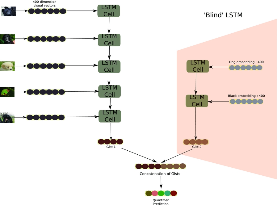
‘Blind’ LSTM: A graphic representation of LSTM is provided in Figure 6 (pink box). This model receives as input the linguistic embeddings for each query. Then, the input is processed by an LSTM module with two cells, which we assume might simulate the composition of the restrictor and scope components of the query; its output is linearly mapped into a five-dimension vector. A softmax classifier is applied on top of this vector in order to output the correct quantifier.
Graphic representation of the CNN+LSTM model.

CNN+LSTM:. As shown in Figure 6, CNN visual features are processed by an LSTM, with the output of the last cell (Gist1) being combined with the linguistic information provided by the ‘Blind LSTM’ module processing the query (Gist2). Gist1 and Gist2 are concatenated into a single vector on top of which a softmax classifier is applied to output the quantifier with the highest probability.
5.4 The role of attention mechanisms: SAN
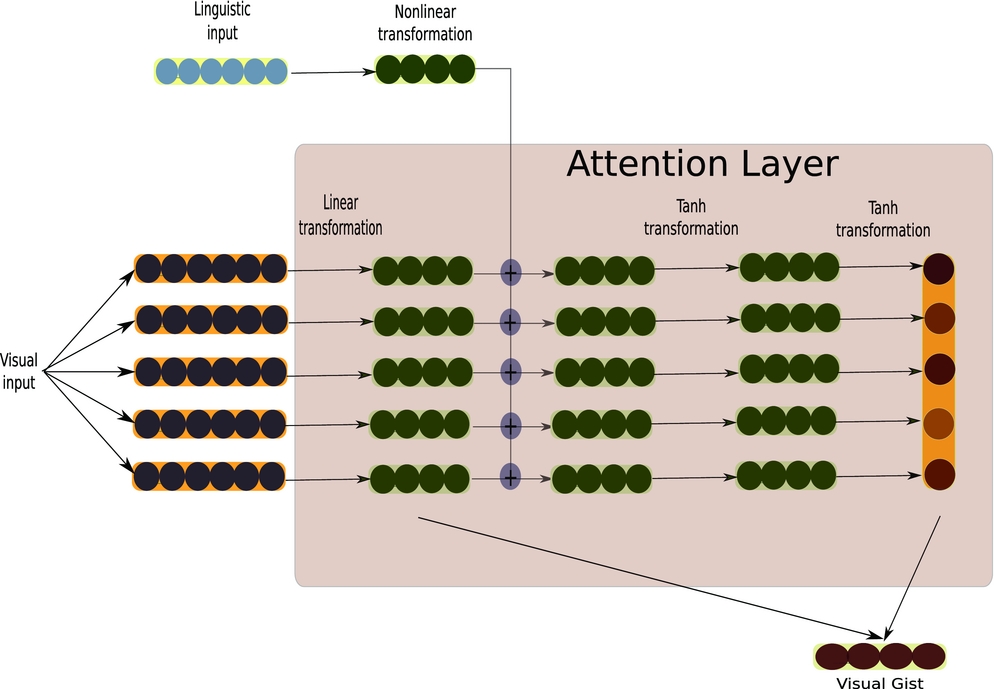
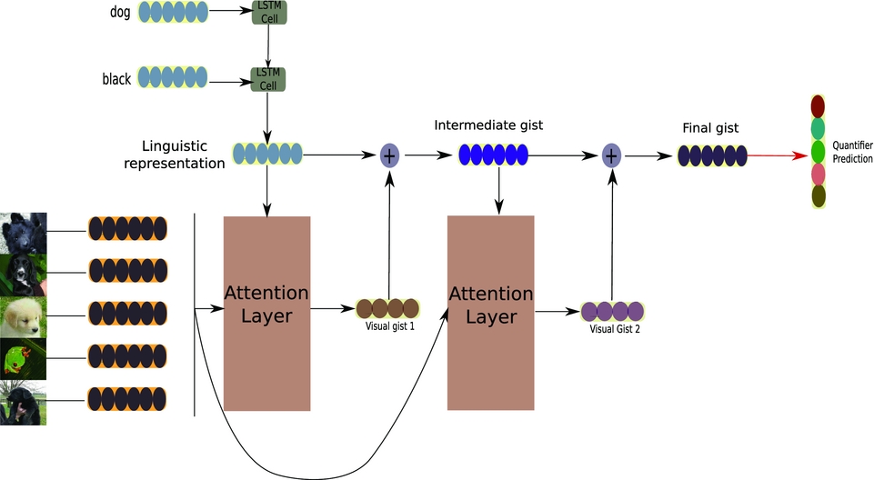
SAN: The SAN proposed by Yang et al. (Reference Yang, He, Gao, Deng and Smola2015) is motivated by the idea that VQA might require more than one step of reasoning. The model is supposed to pay particular attention to the image regions that are relevant to the query via the attention layer. The diagram presented in Figure 7 zooms into the main module of the network: the attention layer. This layer sums each visual vector with the linguistic representation and then applies a tanh and softmax functions to the result, to obtain a weighted average of the initial visual vectors (gist). The gist thus encodes information about both the question and the image. In consistence with the purpose of this architecture, namely performing a multistep reasoning, the attention layer is used twice in SAN. As shown in Figure 8, a first pass applies the representation of the query, as obtained from an LSTM module, to the visual input. In the second pass, the main module takes as linguistic input the sum of the original linguistic representation and the output from the first pass. The final gist is then fed into a softmax classifier to obtain the predicted quantifier.
Graphic representation of the SAN’s attention layer.

Graphic representation of SAN model.

In our experiments, we make a small change to the original SAN architecture and replace the softmax with a tanh function. This choice was motivated by our task, which calls for an attention module able to focus on potentially many objects in the scenario, rather than one or two image regions. (In a scenario containing many objects matching the restrictor, we need the attention to be relatively ‘spread out’ across the image.) Initial experiments supported this hypothesis, and we decided as a result to use tanh for the rest of our experiments (including those on the QSAN model – see Section 5.6).
5.5 The role of formal linguistic structure: QMN
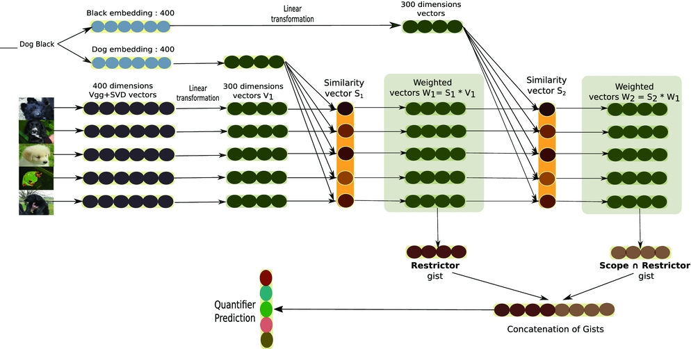
This model is an adaptation of the Memory Network originally proposed by Sukhbaatar et al. (Reference Sukhbaatar, Szlam, Weston and Fergus2015), which achieved state-of-the-art performance in both synthetic question answering and language modelling. The model is shown in Figure 9. Its main feature is that it explicitly encodes the retrieval of the two sets assumed by the formal semantics model of quantifiers (i.e., the restrictor and the overlap between restrictor and scope). This model implements our idea of a quantification model in two steps, where the first step produces some representation of the relevant sets of individuals, and the second step computes the relation between those sets (see Section 1).
A representation of the Quantification Memory Network (QMN) model.

Step 1: As shown in the diagram, the visual and linguistic vectors of all datapoints are linearly mapped to a 300-dimensional space. The 300-dimensional visual vectors are fed into memory cells (V1 in Figure 9); for each cell, we compute the similarity value between each visual vector and the linguistic vector representing the query restrictor (e.g., dog), by calculating their dot product further normalised using the Euclidean norm. The result is either a twenty-two- (for the Q-COCO) or sixteen-dimensional ‘Similarity Vector 1’ (S1) (for Q-ImageNet scenarios). We then calculate the weighted vectors W1 for each individual by multiplying the memory cells V1 with the associated similarity values in S1. This gives us a representation of the amount of ‘dogness’ in each object. The representation of the restrictor set is calculated by summing the memory cells of the weighted vectors obtaining the Restrictor gist. It represents how much ‘dogness’ is found in the given scenario. We then calculate the dot product between the weighted vectors (W1) and the scope linguistic vector (e.g., black), and further normalise the values using the Euclidean norm. Again, the result is a twenty-two- or sixteen-dimensional ‘Similarity Vector 2’ (S2). A second weighted vector W2 is obtained by multiplying W1 and S2. This gives us the amount of ‘black-dogness’ in each object. The representation of the overlap between the restrictor and scope sets (Scope ∩ Restrictor gist) is obtained by summing the new weighted vectors in the memory cells. It represents how much ‘black-dogness’ is found in the given scenario. In this model, the composition of the restrictor and scope components, operationalised in the SAN model by the LSTM module, is accomplished by using the probability of the similarity vector S2 to weight its visual vectors W1.
Step 2: The Restrictor and Scope ∩ Restrictor gists are concatenated into a single 600-dimensional vector that is further linearly transformed into a five-dimensional vector. We apply a softmax classifier on top of the resulting vector that returns the probability distribution over the quantifiers. From the concatenation of the Restrictor gist (dogness) and Scope ∩ Restrictor gist (black-dogness), the model should learn the ratio between the target objects and the restrictor and predict the quantifier that captures that relation.
5.6 Putting it all together: QSAN
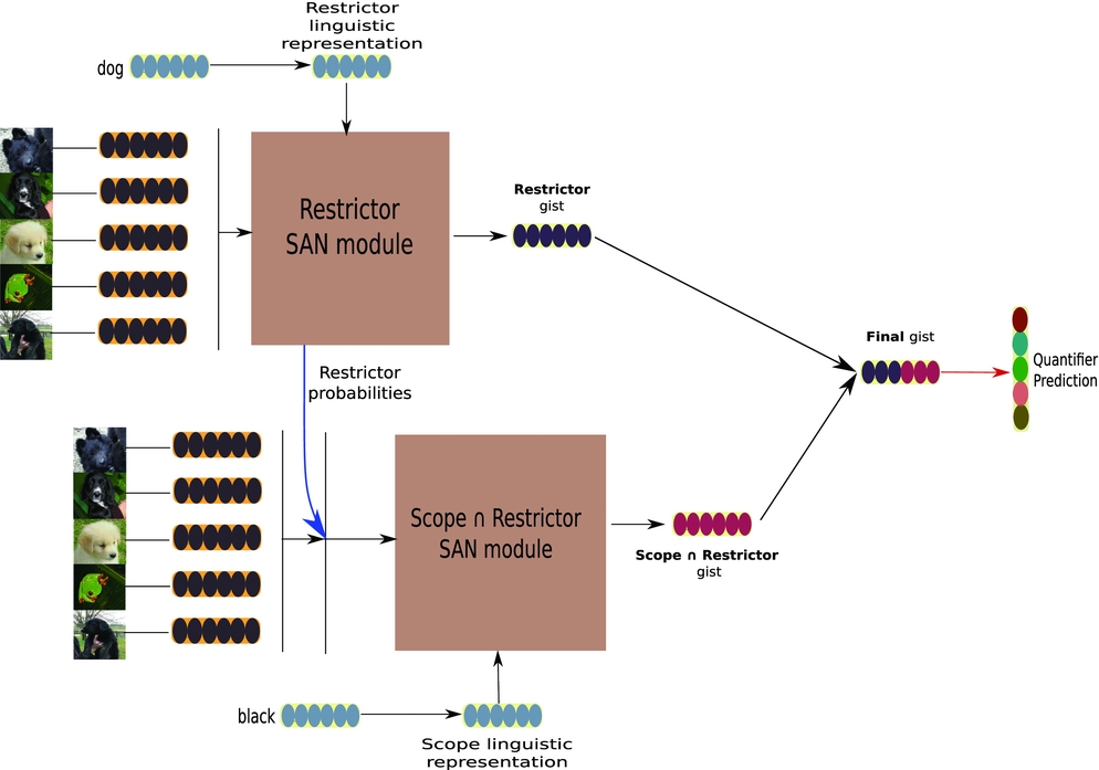
Our QSAN (Figure 10) is an adaptation of SAN integrating the linguistically informed structure of the QMN. The system follows two steps, as in the QMN.
Graphic representation of QSAN model.

Step 1: The SAN model is re-implemented, with the main difference that the given linguistic information is only the restrictor, e.g., the embedding for the word dog. We refer to this part of the model as Restrictor SAN module, and its output as Restrictor gist. The network then takes the probabilities obtained from the softmax layer in the Restrictor SAN module, and uses these probabilities to weight the initial visual vectors. We assume this operation will attend to the correct regions of the visual scenario to find the restrictor set (e.g., the dogs in the image). As in the QMN, the composition of the restrictor and scope is obtained by weighting the visual vectors of the BBs with the restrictor probability before feeding them to the Scope Module. The weighted visual vectors are then fed into the Scope ∩ Restrictor SAN module, where they are processed with respect to the scope’s embedding (e.g., black). The output of this module is the Scope ∩ Restrictor gist.
Step 2: Restrictor and Scope ∩ Restrictor gists are concatenated into a single vector on the top of which a softmax layer is applied to predict the quantifier.
6 Results and analysis
In this section, we report results obtained by all models described in Section 5 in all experimental settings described in Section 4. We then take a closer look using quantitative and qualitative methods of analysis with the aim of gaining a better understanding of the results.
6.1 Results
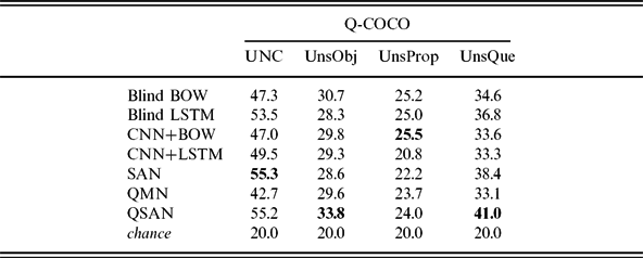
Results for all models in the Q-COCO settings are reported in Table 3. Starting from UNC, we notice that SAN and QSAN are the best-performing models, reaching an accuracy of 55.3 per cent and 55.2 per cent, respectively. However, a very similar performance is obtained by the ‘blind’ LSTM model (53.5 per cent), with the even simpler ‘blind’ BOW achieving remarkably good results (47.3 per cent). This outcome is consistent with our previous discussion on the bias of this dataset towards the linguistic modality. That is, models capitalising solely on linguistic associations between objects and properties are similarly effective as relatively complex state-of-the-art models which integrate both modalities. In other words, adding visual information only marginally contributes to obtain accuracy improvements in this setting. As expected, language-only models are particularly effective in predicting no and all, cases for which object–property distributional associations might intuitively play a bigger role compared to the other quantifiers. To illustrate, the ‘blind’ LSTM achieves sixty-four per cent accuracy for no and seventy-one per cent accuracy for all.
Accuracies of the various models against the Q-COCO dataset

In the UnsProp setting, accuracy for all models is around chance level. To recap, in this setting, we train the models with twenty-nine properties and we test them with fifteen unseen properties. As can be seen in Table 3, none of the models is able to generalise to unseen properties. This confirms that the task is really challenging and it suggests that the visual information provided by CNN features tuned for the task of object classification might not be very informative as far as properties are concerned. This intuition is partially confirmed by the results for UnsObj (models are trained with nineteen and ten objects, respectively), where accuracies increase up to 33.8 per cent (QSAN). Even though the performance of blind models is very close to that of the best-performing QSAN model, it should be noted that generalising over unseen objects is a slightly more feasible task compared to unseen properties. Moreover, the improvement obtained by all models might be indicative of an object bias encoded in the visual vectors.
In the final setting, UnsQue (276 queries in the training data, 118 in the testing data), QSAN is again the best model (41.0 per cent), followed by SAN (38.4 per cent) and the ‘blind’ LSTM (36.8 per cent). The gap between the best attention network and all other models suggests that QSAN is to some extent able to generalise to unseen queries. In contrast, the accuracy of the blind models is over ten per cent lower compared to UNC, thus indicating the poor predictive power of these models when the 〈object, property〉 query has not been seen in training.
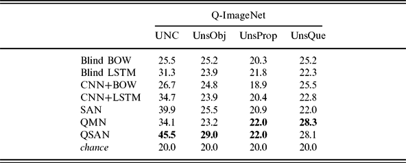
Moving to the Q-ImageNet dataset, we observe in Table 4 that (1) this dataset is harder than Q-COCO, since all accuracies are generally lower across all settings; (2) attention models, i.e., QSAN and SAN, turn out to be best overall, across all best settings, with QSAN outperforming SAN and with QMN being slightly worse than SAN in two settings and slightly better in the other two. This confirms the crucial role of using the restrictor to guide the attention through the image (and then compose) instead of composing restrictor and scope at the linguistic level only, as done by the LSTM model. In particular, QSAN model is the best-predicting model in three settings out of four, namely the UNC, UnsObj and UnsProp (same performance as QMN), and the second-best in UnsQue. SAN is worse than QSAN in UNC and UnsObj, but better than QMN. Finally, QMN slightly outperforms QSAN in UnsQue.
Accuracies of the various models against the Q-ImageNet dataset

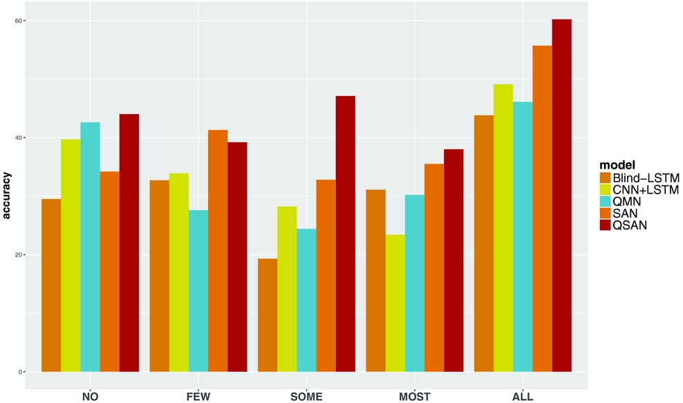
Starting from UNC setting, Table 4 shows that QSAN outperforms SAN by almost six per cent and the CNN+LSTM by more than ten per cent. A visual representation of such results is provided in Figure 11, which shows the accuracies of the five best-performing models relative to each quantifier. As can be noticed, the QSAN model outperforms the other models for no, some, most and all, whereas few is best predicted by SAN. At first glance, it can be noted that on average, the accuracies of QSAN are more constant across the quantifiers, whereas all the others have some drops corresponding to specific quantifiers (see, e.g., the fairly low accuracy for some obtained by SAN).
UNC Q-ImageNet. Accuracies of five best-predicting models relative to each quantifier.

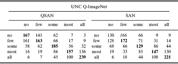
In Table 5, we report a quantitative analysis of the errors made in UNC by QSAN and SAN. The first thing to be noticed is that QSAN correctly predicts the target quantifier (in bold) more often than it predicts the wrong ones. In contrast, that does not hold for SAN, which predicts few more often than no when no is the target quantifier. Second, errors made by QSAN are always ‘plausible’, meaning that the network – when wrong – tends to predict quantifiers that are adjacent to the target one. That is, it wrongly outputs most more often than some, few and no (in this order), when the target quantifier is all. In contrast, errors in SAN do not follow the same pattern: for example, the network outputs no more often than few when the correct quantifier is some.
Confusion matrices for QSAN and SAN in UNC Q-ImageNet

As far as the other settings are concerned, a similar pattern of results as the one described for Q-COCO is observed (see Table 4). In particular, all models are around chance level for UnsProp (models trained with 113 objects, tested with forty eight) and slightly better for UnsObj (models trained with fourteen properties, tested with eight), where QSAN is the best-performing system (29.0 per cent), followed by the other attention model, SAN (25.5 per cent). In contrast with Q-COCO, where some models obtain fairly high accuracies in the UnsQue setting, in this dataset, none of the models reaches thirty per cent accuracy (models trained with 893 queries, tested with 351). QMN and QSAN are however the best (28.3 per cent) and second-best (28.1 per cent), respectively. The gap between the two datasets is probably due to the highest repetition of objects in Q-COCO compared to Q-ImageNet due to the comparably much lower number of object categories that are included (twenty nine compared to 161). Even though the properties are almost halved in the latter compared to the former (24 versus 44), we conjecture that the lower number of object categories in Q-COCO plays a crucial role in helping any model to better ‘recognise’ a given object in a scenario. Thus, seeing the same object more often in training (as in Q-COCO) should help more than seeing the same property more often (as in Q-ImageNet).
6.2 Analysis
To better understand the results obtained with QSAN, we perform two kinds of analysis. The first is aimed at testing whether the task of predicting the correct quantifier is harder when the scenario contains an increasing number of distractors having the same queried property. For instance, if the query is black dog, it could be the case that the model is confounded when a high number of black objects (i.e., black non-dogs) is present amongst the distractors. We check this by computing the total number of cases for each cardinality of distractors with the queried property (i.e., the number of black non-dogs) as well as the number of cases that are correctly predicted by QSAN in Q-ImageNet UNC for each cardinality. As the proportion of correctly predicted cases is constant across the various cardinalities, this factor does not seem to affect the model’s performance.
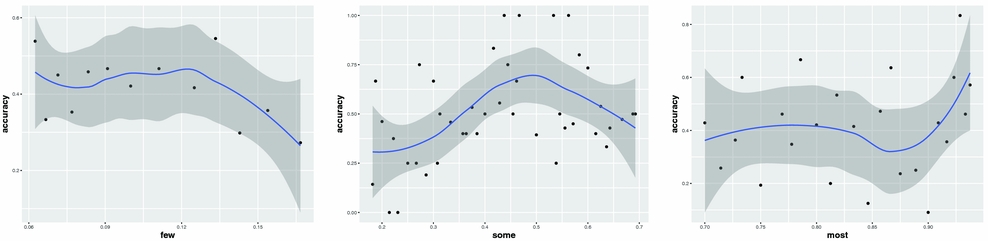
The second analysis is aimed at checking whether the accuracy of QSAN in Q-ImageNet UNC is affected by the actual ratio of targets over restrictor objects. Our hypothesis is that the model might be confounded when ratios that are at the boundaries between different quantifiers (e.g., across seventy per cent, that defines the boundary between some and most), while it should perform better when the ratio is undoubtedly associated with a given quantifier (e.g., around forty-three per cent for some). When analysing the model’s accuracy with respect to the whole span of ratios ranging from zero per cent to hundred per cent, we do not find such clear ‘peaks’. Accordingly, model’s predictions are stable across quantifiers (and relative ratios), as shown in Figure 11. However, it could be the case that local patterns of fluctuation can be found within each quantifier’s ratios. This is clear in Figure 12, where we zoom into few (left), some (centre) and most (right), which are the three that are defined by ranges. It can be seen that, the expected trend is clearly visible in these plots. In particular, a peak can be observed for few and some, with most having a slightly fuzzier fluctuation, that is however still consistent with our hypothesis.
QSAN. Accuracy in UNC plotted against the ratios of target objects over restrictors. Left: ‘few’. Center: ‘some’. Right: ‘most’.

A third, more general analysis, aims at understanding to which extent quantification is made harder by having to deal with ‘real’ concepts and images. What we wish to check is whether the purely logical part of the quantifier, which computes a ratio between two sets, can easily be learnt by a network. To do this, we reduce the uncontrolled Q-ImageNet dataset to its simplest instance, as white dots (corresponding to the intersection between restrictor and scope) and black dots (corresponding to the restrictor), in images with a gray background.
We then build a simple classifier over this data, by training from scratch a shallow CNN, with just one convolution layer. This system obtains ninety-six per cent accuracy, confirming NNs can learn the quantification comparison step nearly perfectly if a completely abstract representation is given. This is an interesting result which confirms that the actual challenge of visual quantification is to find the right strategies to deal with uncertainty in object and property recognition. As the psycholinguistic literature shows, humans appeal extensively to their ANS to quantify (see Section 2). This may be more than an efficiency mechanism: as demonstrated by the QSAN model’s combination of soft attention and gist, approximation goes a long way in manoeuvring through the difficulties of matching words and vision.
7 Conclusion
In this paper, we investigated the task of quantifying over visual scenes using natural language quantifiers. We argued that the task is considerably different from prior work in language and vision, in that it requires both the ability to match linguistic constituents to areas of an image, and the capacity to abstract over the nature and cardinality of the identified entities to compute an appropriate quantification class.
Our main contribution is a new insight into the architectural requirements of a quantification system. We first showed that letting the network compose scope and restrictor on the language side, and using this representation to attend to the image, resulted in underperforming models. Instead, using the linguistic representation of the quantifier as a relation between sets, guiding the attention mechanism, produced much better accuracy, as illustrated by the QMN and QSAN models. We take this result to show that, when considering complex, high-level phenomena, it is useful to correlate insights from formal linguistics with targeted NN mechanisms. We hope that our study will encourage further work in building linguistically motivated neural architectures.
Furthermore, in order to perform the experiments reported in this work, we built a novel dataset of image scenes paired with linguistic queries that the system is tasked to quantify. We showed that such a dataset is difficult to build in a balanced way when relying on large datasets of real images. We suggested a strategy involving the construction of visual scenarios made of existing BBs, assembled together in a balanced manner. The dataset is freely available at https://quantit-clic.github.io/
Our error analysis highlighted an interesting property of the QSAN model, namely that the model performs better on those proportions which are clearly associated with a given quantifier and falters at the boundary between two quantifiers. This is appropriate behaviour for our simplified setting, where quantifiers are paired with fixed, somewhat arbitrary proportions. Basically, the system starts ‘hesitating’ at the arbitrary boundary. Further work with fuzzy quantifier classes should follow to test the system in a more realistic setting.
Finally, we highlighted that the computation of a proportion between sets is easily learnable by a neural architecture if it is provided with a gold standard for the identification of the intersection of the scope and restrictor in the image. This demonstrates that the difficulty of the task is in providing an end-to-end solution to the quantification problem, which can cope with failures in object and property identification. We believe that the QSAN’s combination of soft attention and gist, which reproduces the human’s ANS, goes some way towards that goal. Further experiments are however needed to understand the interaction between visual recognition and abstraction modules. In particular, we note recent work by Trott, Xiong and Socher (Reference Trott, Xiong and Socher2017), which models the restriction and scope of cardinals by explicitly counting over the identified objects in the image. The model obtains good improvements on ‘how many’ questions in standard VQA dataset. We leave for further work whether this sequential, counting strategy is appropriate for the type of vague quantifiers we studied in this paper.