NOMENCLATURE

ADS–B

automatic dependent surveillance–broadcast

AMAN

arrival manager

ANSP

air navigation service provider

ATD

actual time of departure

ATM

air traffic management

CART

classification and regression trees

CDM

collaborative decision making

DDR2

EUROCONTROL Demand Data Repository

DNN

deep neural network

ETA

estimated time of arrival

ETMS

enhanced traffic management system

FAA

Federal Aviation Administration

IATA

International Air Transport Association

ICAO

International Civil Aviation Organization

ISG

Istanbul Sabiha Gokcen International Airport

LTBA

Istanbul Atatürk International Airport

MAE

mean absolute error

MCNN

multi-cells neural network

METAR

meteorological aerodrome report

MOJO

model object optimised

MSE

mean squared error

NN

neural networks

OOB

out-of-bag

QRF

quantile regression forests

RF

random forests

RMSE

root mean squared error

RNN

recurrent neural network

SESAR

Single European Sky ATM Research

STA

scheduled time of arrival

STD

scheduled time of departure

TMA

terminal manoeuvring area

2.0 DATA DESCRIPTION

The raw data used for ETA prediction consist of general information about the flight, trajectory points and airport weather reports. The raw data were obtained in different formats (e.g. Automatic Dependent Surveillance-Broadcast (ADS-B), allft+, Meteorological Aerodrome Report (METAR)) from different data sources (e.g. EUROCONTROL Demand Data Repository (DDR2), Iowa State University). Then the data were exported to a relational database which was designed to be able to query and explore the data easily. A Java web application was developed to visualise the data (trajectories, TMA entrances etc.) on the map, which provides further insight into the possible problems and issues related with the data. The features to be used in training the machine learning models were determined depending on the available data, domain knowledge and previous studies. Then, a feature engineering process is employed to remove the missing, inconsistent (e.g. flights with incomplete trajectory points) or duplicate data and to derive new features from available data using data transformations.

2.1 Dataset

The main dataset used in this study consists of arrivals to Istanbul Atatürk International Airport (IST/LTBA) from April 2018 to August 2018. The dataset contains 63,460 commercial flights (both domestic and international), 18,869,049 trajectory points and 6,236 METAR reports for LTBA. Allft+ data for the same period were also obtained from DDR2 and were used to determine the time and co-ordinates of the TMA entrance for each aircraft. Table 1 presents a list of data fields related with the general flight information, flight trajectory and weather around airport.

Table 1

Data fields

Table 2

Timestamp transformation

2.2 Feature engineering

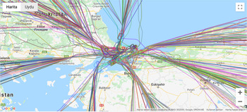
In machine learning projects, it is crucial to convert the raw data into a relational and tidy data format (e.g. a database) to be able to easily explore the relationship among data. Therefore, a relational database was designed to establish the relationship between the data obtained in different formats from different sources. Then, the data were inserted into the database from various data files. A Java web application was developed for data exploration and visualisation purposes. Figure 1 shows the trajectories of arrivals to LTBA for one of the busiest days in the selected period. After a careful data exploration process, flights with missing feature values and duplicate data were removed. Data with inconsistencies (very close TMA and runway arrival times, incomplete trajectories, etc.) were also removed. After data exploration and cleaning, we had 51,902 individual flights in the dataset.

Figure 1.

Trajectories of arrivals to LTBA on 22 July 2018.

Timestamp data are not appropriate for training machine learning models. Therefore, the timestamp data such as scheduled and actual departure/arrival times were converted into two numerical features: ‘day of year’ and ‘minutes passed since midnight’. Table 2 presents examples of this transformation. The aircraft types were grouped into three categories corresponding to International Civil Aviation Organization (ICAO) Wake Turbulence Categories: ‘light’, ‘medium’ and ‘heavy’. More than 90% of the flights in the dataset were operated by national airlines. Therefore, airline categories were grouped into five categories: ‘Turkish Airlines’, ‘Atlas Global’, ‘Onur Air’, ‘Pegasus Airlines’ and ‘Other’.

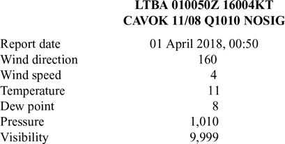
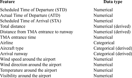
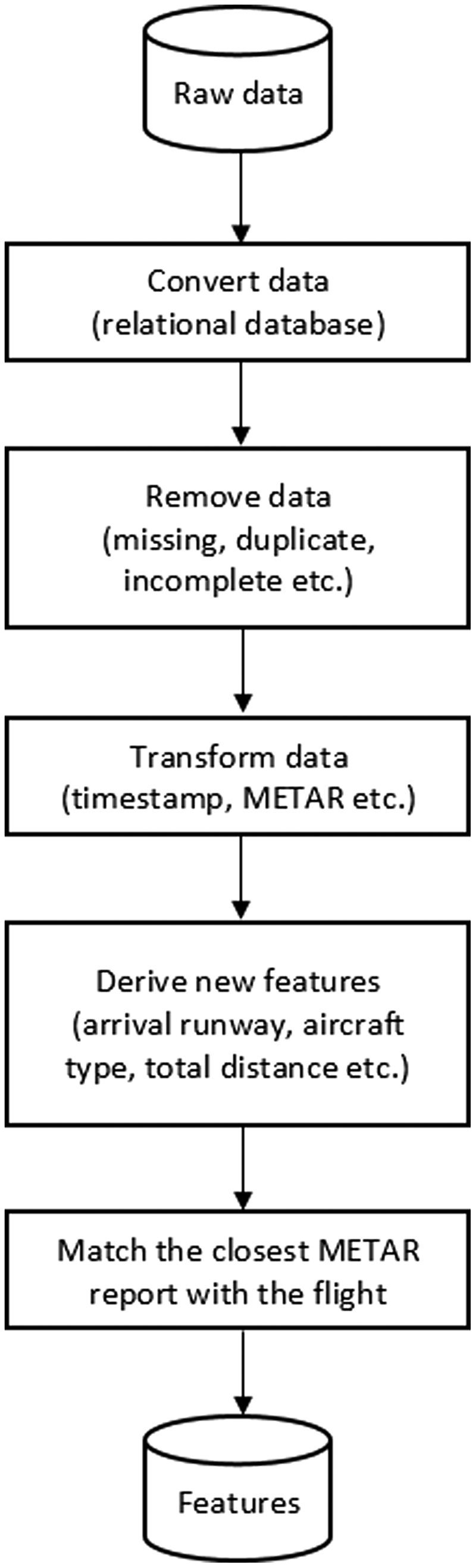
Four additional features were derived from the data: the arrival runway, aircraft type (e.g. ICAO wake turbulence category), total flight distance and the distance from TMA entrance to runway. The arrival runway was determined from the arithmetic average of the headings of final approach trajectory points. The total distance was calculated using the trajectory data. Therefore, the effect of the departure airport was not considered to be the same for all flights departing from the same airport. To calculate the distance from TMA entrance to runway, the co-ordinates of the TMA entrance were determined using allft+ data which contains the airspace entry/exit time and co-ordinates. METAR data were parsed from their original format. METARs closest to the actual arrival times of the corresponding flights were determined and matched with the flight data to reflect the actual weather conditions around the airport at the time of arrival. Table 3 presents an example of METAR conversion, and Table 4 presents the final set of features used for ETA prediction. Figure 2 shows the whole feature engineering process.

Table 3

METAR conversion example

Table 4

Features for ETA prediction

Figure 2.

Feature engineering process.

3.0 METHODOLOGY

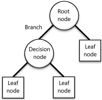
RF and deep neural networks were used for ETA prediction. RF^{(Reference Breiman9)} is an ensemble learning method to build a forest of uncorrelated decision trees using a procedure such as Classification and Regression Trees (CART)^{(Reference Breiman, Friedman, Stone and Olshen12)}, with random split selection^{(Reference Dietterich13)} and bagging^{(Reference Breiman14)}. A decision tree consists of many decision nodes, beginning at the root node and ending at the leaf nodes (Fig. 3). Nodes are connected to sub-nodes with branches which are the possible outcomes of the decisions given at the parent nodes^{(Reference Ghatak15)}. At each decision node $m$, a test function ${f_m}\left( x \right)$ is applied to a given input, and one of the branches is taken depending on the output^{(Reference Alpaydin16)}. This process is repeated until a leaf node is hit. The value of the leaf node is the output.

Figure 3.

Decision tree.

Each decision node uses only one of the input features (${x_j}$) in a univariate tree. If ${x_j}$ is discrete with $n$ possible values, then the decision node will have $n$ splits. The corresponding branch will be selected depending on the value of ${x_j}$. If ${x_j}$ is numeric, then ${f_m}\left( x \right)$ will compare ${x_j}$ with a threshold value ${w_{{m_0}}}$ and divide the input space into two regions. This is called a binary split.

(1) \begin{equation}{L_m} = \left\{ {x{|}{x_j} \gt {w_{{m_0}}}} \right\}\end{equation}

(2) \begin{equation}{R_m} = \left\{ {x{\rm{|}}{x_j} \leq {w_{{m_0}}}} \right\}\end{equation}

Many different decision trees can be constructed for a given training set. Usually, the smallest tree is tried to be found greedily by looking for the best split at each step. In a classification tree, where the output of the decision tree is one of the $p$ classes, the goodness of a split is determined by an impurity measure. In a two-class problem where ${p^1} = p$ and ${p^2} = 1 - p$, the impurity of a split can be measured using a non-negative function $\phi \left( {p,1 - p} \right)$. Some examples of this function are entropy, Gini index and misclassification error, which are respectively defined as:

(3) \begin{equation}\phi \left( {p,1 - p} \right) = - p{\log _2}\ p - \left( {1 - p} \right){\log _2}\left( {1 - p} \right)\end{equation}

(4) \begin{equation}\phi \left( {p,1 - p} \right) = 2p\left( {1 - p} \right)\end{equation}

(5) \begin{equation}\phi \left( {p,1 - p} \right) = 1 - {\rm{max}}\left( {p,1 - p} \right)\end{equation}

In a regression tree, where the output of the decision tree is a numeric value, the goodness of a split is measured by the mean square error from the estimated value.

RF consists of many decision trees where the output of the forest is determined by majority voting or averaging in classification and regression problems, respectively (Fig. 4). RF can handle both continuous and categorical features, and they can run efficiently on large data sets with many features. Additionally, overfitting is prevented with the randomness and the use of decision trees as an ensemble. Each tree in the RF is grown using random samples of the training data. This is called bagging. The samples that are excluded in the training process are called ‘Out-Of-Bag’ (OOB) samples. They can be used to get unbiased prediction error estimates and produce feature importance estimates^{(Reference Kern, Medeiros and Yoneyama4)}. At each node, the split is selected randomly among the K best splits.

Figure 4.

Random forests.

The characteristics of RF are as follows^{(Reference Breiman9)}:

1. i. RF is robust to outliers and noise.

2. ii. RF works faster than bagging or boosting.

3. iii. RF provides useful estimates of error, variable importance and correlation.

4. iv. RF is simple and comprehensible.

The term ‘deep learning’ was introduced by Dechter in 1986^{(Reference Dechter17)}. It was first mentioned in Neural Networks (NNs) by Aizenberg et al. in 2000^{(Reference Aizenberg, Aizenberg and Vandewalle18)}. Deep learning is the state-of-the art method in speech recognition, visual object recognition, object detection, etc. Deep learning models consist of multiple layers which reveal the complex relationships in large data sets and learn the representations of data using the backpropagation algorithm^{(Reference Lecunn, Bengio and Hinton19)}.

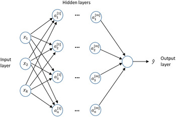
At each layer, deep learning methods transform the current representation into a more abstract representation. Very complex functions can even be learned with such transformations. Figure 5 shows the representation of a deep neural network with $k$ input features, $m$ hidden layers and $n$ neurons (nodes) in each hidden layer. Each node in the deep neural network corresponds to a computational unit that takes the weighted sum of node inputs and passes the result to a non-linear activation function to calculate the output of that node (Fig. 6). Nodes that are not in the input or output layer are called hidden nodes. Deep neural networks (DNNs) are the neural networks with multiple hidden layers.

Figure 5.

Neural network representation.

Figure 6.

Structure of a single neuron.

Here,

\begin{equation*}x = {\left[ \begin{array}{ccc}x_{{\rm 1}} & x_{{\rm 2}} & \begin{array}{cc}{\rm \dots } & x_k \end{array} \end{array}\right]}^T = \mathrm{feature\ vector},\end{equation*}

\begin{equation*}w = {\left[ \begin{array}{ccc}w_{{\rm 1}} & w_{{\rm 2}} & \begin{array}{cc}{\rm \dots } & w_k \end{array} \end{array}\right]}^T = \mathrm{weight\ vector},\end{equation*}

$b$ = bias vector,

$a$ = activation function

Some of the non-linear activation functions are as follows:

(6) \begin{equation}{{{f}}}\!\left({{{z}}}\right) = {{\text{max}} \left({0},{{{z}}}\right)\ }{\rm \ (}{{{ReLU}}})\end{equation}

(7) \begin{equation}{{{f}}}\!\left( {{{z}}} \right) = \frac{{{{{{e}}}^{{{z}}}} - {{{{e}}}^{ - {{{z}}}}}}}{{{{{{e}}}^{{{z}}}} + {{{{e}}}^{ - {{{z}}}}}}}{\rm{\;}}\left( {{{tanh}}} \right)\end{equation}

(8) \begin{equation}{{{f}}}\!\left( {{{z}}} \right) = \frac{{1}}{{{1} + {{{{e}}}^{ - {{{z}}}}}}}{\rm{\;}}\left( {{{sigmoid}}} \right)\end{equation}

(9) \begin{equation}f\left( z \right) = z\;\left( {identity} \right)\end{equation}

Equations (10)–(16) define the procedure to calculate the predicted output of the deep neural network shown in Fig. 5 starting with the layer 1 through layer $\textbf{\textit{m}}$.

(10) \begin{equation}{{{{z}}}^{\left[ {1} \right]}} = {{{{W}}}^{\left[ {1} \right]}}{{{x}}} + {{{{b}}}^{\left[ {1} \right]}}\end{equation}

(11) \begin{equation}{{{{a}}}^{\left[ {1} \right]}} = {{{f}}}\!\left( {{{{{z}}}^{\left[ {1} \right]}}} \right)\end{equation}

(12) \begin{equation}{{{{z}}}^{\left[ {2} \right]}} = {{{{W}}}^{\left[ {2} \right]}}{{{{a}}}^{\left[ {1} \right]}} + {{{{b}}}^{\left[ {2} \right]}}\end{equation}

(13) \begin{equation}{{{{a}}}^{\left[ {2} \right]}} = {{{f}}}\!\left( {{{{{z}}}^{\left[ {2} \right]}}} \right)\end{equation}

(14) \begin{equation}{\rm \ }z^{\left[m\right]} = W^{\left[m\right]}a^{{\rm [}m{\rm -1]}} + b^{\left[m\right]}\end{equation}

(15) \begin{equation}{\rm \ }a^{{\rm [}m{\rm ]}} = f\!\left(z^{{\rm [}m{\rm ]}}\right)\end{equation}

(16) \begin{equation}\hat{y} = f(a^{[m]})\end{equation}

Here $\hat{y}$ is the output vector.

Figure 7.

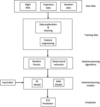
ETA prediction approach.

Simple stochastic gradient descent can be used to train multi-layer architectures. Gradients can be computed using the backpropagation algorithm. The backpropagation algorithm is actually a practical application of the chain rule for derivatives to calculate the parameters of the model ($W,b$) that minimise the prediction error.

Figure 7 shows the steps of the proposed ETA prediction approach. Raw flight, trajectory and weather data are filtered and formatted by data exploration and cleaning, and then training data were obtained through feature engineering processes. RF and DNN algorithms were used to train and test machine learning models. ReLU activation function given in Equation (6) and identity activation function given in Equation (9) were used in the hidden and output layers of DNN, respectively. These models were then used in an application to predict the ETA using any input data.

MAE, Mean Squared Error (MSE) and Root Mean Squared Error (RMSE) metrics given in Equations (17)–(19) are used to evaluate the performance of ETA prediction models.

(17) \begin{equation}{\rm MAE} = \frac{{\rm 1}}{n}\sum^n_{i{\rm =1}}{\left|\widehat{y_i}{\rm -}y_i\right|}\end{equation}

(18) \begin{equation}{\rm MSE} = \frac{{\rm 1}}{n}\sum^n_{i{\rm =1}}{{{\rm (}{\hat{y}}_i{\rm -}y_i{\rm )}}^{{\rm 2}}}\end{equation}

(19) \begin{equation}{\rm RMSE} = \sqrt{\frac{{\rm 1}}{n}\sum^n_{i{\rm =1}}{{{\rm (}{\hat{y}}_i{\rm -}y_i{\rm )}}^{{\rm 2}}}}\end{equation}

where $n = $ number of observations, ${\hat{y}_i} = i-{\text{th}} $ predicted value and ${y_i} = $ the i-th observed value of ETA.

Table 5

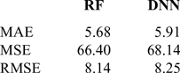
Results for ETA prediction after departure (LTBA)

Table 6

Results for ETA prediction after TMA entry (LTBA)

Figure 8.

Error histograms after departure and after TMA entrance using (A) RF and (B) DNN.

4.0 EXPERIMENTAL RESULTS AND DISCUSSION

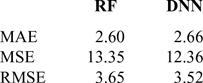
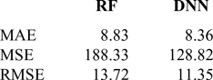
RF and deep neural networks were implemented in R programming language using h2o package, an open source, distributed and scalable machine learning platform⁽²⁰⁾. As mentioned in Section 2.2, flight information data, trajectory data and METAR data for LTBA were used for training the machine learning models. The data were randomly split into training (80%) and test data (20%). The performances of machine learning models were evaluated using various parameter values. Parameters for RF were chosen as number of split features = 6 and the number of trees = 200. Parameters for deep learning were chosen as number of epochs = 100, number of hidden layers = 2 and number of neurons per hidden layer = 40. A quad-core computer with a 2.80GHz processor and 6GB memory was used for training and running the model. Training took less than 3min. Tables 5 and 6 show the evaluation metrics for ETA prediction using RF and DNN after departure and TMA entry, respectively. ETAs after TMA entrance can be predicted with a MAE less than 3min, while ETAs after departure can be predicted with a MAE less than 6min. Machine learning models decreased the prediction errors 64% after departure and 84% after TMA entrance with respect to scheduled time of arrival. Figure 8 shows the error histograms for ETA prediction using RF and DNN. The bars entitled ‘Scheduled-Actual’ in the error histograms represent the error between the scheduled time of arrival and the actual time of arrival. The horizontal axis represents the error in minutes, while the vertical axis represents the number of flights. The bars entitled ‘Predicted-Actual’ represent the error between the time of arrival predicted by the machine learning models and the actual time of arrival. The error histograms clarify that predictions calculated by the machine learning models concentrate around a narrow vicinity of 0, where ‘0’ means an exact match with the actual time of arrival. It is much clearer in the error histograms for the predictions calculated after TMA entrance, where it can be seen that more than 90% of the errors are between −5min and 5min. On the contrary, the errors between the scheduled and actual time of arrivals spread a very wide range around zero, where the distribution of errors is right-sided, which means that late arrivals are much greater in number than early arrivals.

Machine learning models were also used to predict the ETA after departure for another airport (Istanbul Sabiha Gokcen International Airport – ISG) with similar runway configuration. Table 7 shows the evaluation metrics for ISG. Both models succeeded to predict ETAs with a MAE less than 9min for an airport which was not included in the training process at all.

Table 7

Results for ETA prediction after departure (ISG)

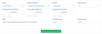
Machine learning models were obtained as ‘h2o MOJO (Model ObJect, Optimized) models’, which are intended to be easily embeddable in any Java environment.  Then, the MOJOs were integrated into a Java web application developed for ETA prediction. Both models are able to predict the ETA in less than 5s. Figure 9 shows a screenshot of the ETA prediction for a sample flight where the actual time of arrival for is 20:55 UTC and scheduled time of arrival is 21:05 UTC. Thus, ETAs for any flights can be predicted dynamically by providing the required feature values.

Figure 9.

ETA prediction on the application.