1 Introduction
Turbulent fluid flows with large near-wall gradients of thermo-physical properties can occur in a wide range of engineering applications, where strong wall heat transfer plays an important role. The mean velocity and near-wall turbulent structures are greatly affected by near-wall gradients of, e.g., density
 $\unicode[STIX]{x1D70C}$
and viscosity
 $\unicode[STIX]{x1D707}$
. However, the majority of studies on turbulent flow structures have been performed for constant-property flows.
The existence of near-wall turbulent structures has been known for several decades, and their structural features have been investigated in great detail. Although geometrically thin, the near-wall region that is formed by the viscous and buffer layers is responsible for a large fraction of the velocity drop (Jiménez & Moser Reference Jiménez and Moser2007). This shear-dominated near-wall region accounts for a significant amount of turbulence production across the boundary layer and thus plays a crucial role in skin friction and heat transfer. The dominant structures of the near-wall region are streamwise velocity streaks and quasistreamwise vortices. Streaks (Kline et al. Reference Kline, Reynolds, Schraub and Runstadler1967) are spanwise modulation of streamwise velocity and consist of low- and high-speed streaks with a characteristic spacing of approximately 100 wall units in the spanwise direction (Smith & Metzler Reference Smith and Metzler1983). The quasistreamwise vortices, primarily found in the buffer layer, are slightly inclined away from the wall and tilted in spanwise directions (Jeong et al. Reference Jeong, Hussain, Schoppa and Kim1997). Additionally, it is known that the dynamics of near-wall turbulence can be maintained autonomously by a self-sustaining process, where the streaks and the vortices continue to regenerate each other independently of the outer flow (Jiménez & Pinelli Reference Jiménez and Pinelli1999). According to Hamilton, Kim & Waleffe (Reference Hamilton, Kim and Waleffe1995), the sustainment of near-wall turbulence involves a closed-loop mechanism whereby the generation of streaks is induced by quasistreamwise vortices that are in turn created by streak instability. An alternate description of the self-sustaining mechanism has been provided by Chernyshenko & Baig (Reference Chernyshenko and Baig2005), in which the physical mechanism of streak formation is related to the combined action of wall-normal motions, mean shear and viscous diffusion. While there are differences in the interpretation of the self-sustaining process, a close relation between low-speed streaks and quasistreamwise vortices is well established (Robinson Reference Robinson1991; Jeong et al. Reference Jeong, Hussain, Schoppa and Kim1997; Jiménez & Pinelli Reference Jiménez and Pinelli1999; Kim & Lim Reference Kim and Lim2000; Schoppa & Hussain Reference Schoppa and Hussain2002) and is also supported by self-sustaining mechanisms described by Hamilton et al. (Reference Hamilton, Kim and Waleffe1995) and Chernyshenko & Baig (Reference Chernyshenko and Baig2005).
The near-wall coherent structures for variable-property wall turbulence have been far less explored in the past. Recently, Zonta, Marchioli & Soldati (Reference Zonta, Marchioli and Soldati2012) and Lee et al. (Reference Lee, Yoon Jung, Jin Sung and Zaki2013) have investigated incompressible flows with near-wall viscosity gradients and found that the turbulent structures are affected by these gradients. Further knowledge on variable-property effects on turbulent structures has been provided by experimental and numerical studies of supersonic flows with adiabatic walls (e.g. Spina & Smits Reference Spina and Smits1987; Pirozzoli, Bernardini & Grasso Reference Pirozzoli, Bernardini and Grasso2008; Ringuette, Wu & Martin Reference Ringuette, Wu and Martin2008; Elsinga et al.
Reference Elsinga, Adrian, Van Oudheusden and Scarano2010; Lagha et al.
Reference Lagha, Kim, Eldredge and Zhong2011b
), and cooled or heated walls (e.g. Coleman, Kim & Moser Reference Coleman, Kim and Moser1995; Lechner, Sesterhenn & Friedrich Reference Lechner, Sesterhenn and Friedrich2001; Foysi, Sarkar & Friedrich Reference Foysi, Sarkar and Friedrich2004; Morinishi, Tamano & Nakabayashi Reference Morinishi, Tamano and Nakabayashi2004; Duan, Beekman & Martin Reference Duan, Beekman and Martin2010; Lagha et al.
Reference Lagha, Kim, Eldredge and Zhong2011a
; Shadloo, Hadjadj & Hussain Reference Shadloo, Hadjadj and Hussain2015; Modesti & Pirozzoli Reference Modesti and Pirozzoli2016). Experimental studies on supersonic boundary layer structures are limited to the investigation of large-scale motions in the outer region of the flow, while numerical studies additionally allow a detailed investigation of near-wall structures. For supersonic boundary layers with adiabatic walls, the dynamics of near-wall turbulent structures is found to be similar to that of constant-property cases, and its characteristics scale well with the classical wall-based scaling (Pirozzoli et al.
Reference Pirozzoli, Bernardini and Grasso2008; Ringuette et al.
Reference Ringuette, Wu and Martin2008; Lagha et al.
Reference Lagha, Kim, Eldredge and Zhong2011a
). For cooled walls, the near-wall streaks extend in the streamwise direction (Coleman et al.
Reference Coleman, Kim and Moser1995; Duan et al.
Reference Duan, Beekman and Martin2010; Lagha et al.
Reference Lagha, Kim, Eldredge and Zhong2011a
), while they shorten for heated walls (Lagha et al.
Reference Lagha, Kim, Eldredge and Zhong2011a
). These streak modifications were quantified in terms of wall-based viscous units. The semilocal scaling (Huang, Coleman & Bradshaw Reference Huang, Coleman and Bradshaw1995), which uses the wall shear stress
 $\unicode[STIX]{x1D70F}_{w}$
and local properties to define near-wall scales, has been shown to be effective to account for changes in streak length in the buffer layer (Morinishi et al.
Reference Morinishi, Tamano and Nakabayashi2004; Patel et al.
Reference Patel, Peeters, Boersma and Pecnik2015). Even though the semilocal scaling is able to account for some of the differences seen between non-adiabatic variable- and constant-property flows, it has not been able to provide a universal scaling law. For instance, in a supersonic channel flow with cold isothermal walls, an increase in turbulence to mean time scale ratio was reported by Coleman et al. (Reference Coleman, Kim and Moser1995) and a reduced pressure–strain rate resulting in an increased turbulence anisotropy was noted by Foysi et al. (Reference Foysi, Sarkar and Friedrich2004). In a more recent study, Modesti & Pirozzoli (Reference Modesti and Pirozzoli2016) performed direct numerical simulation (DNS) at different Reynolds and Mach numbers for compressible isothermal channel flows, and they noted an increase of streamwise turbulence intensity with Mach number as a dominant variable-property effect.
The van Driest transformed mean velocity
 $\overline{u}^{vD}=\int _{0}^{\overline{u}/u_{\unicode[STIX]{x1D70F}}}\sqrt{\overline{\unicode[STIX]{x1D70C}}/\overline{\unicode[STIX]{x1D70C}}_{w}}\,\text{d}(\overline{u}/u_{\unicode[STIX]{x1D70F}})$
, when plotted as a function of
 $y^{+}=yRe_{\unicode[STIX]{x1D70F}}/h$
, has been successful in collapsing velocity profiles of supersonic flows over adiabatic walls with velocity profiles from constant-property flows (Guarini et al.
Reference Guarini, Moser, Shariff and Wray2000; Maeder, Adams & Kleiser Reference Maeder, Adams and Kleiser2001; Duan, Beekman & Martin Reference Duan, Beekman and Martin2011; Lagha et al.
Reference Lagha, Kim, Eldredge and Zhong2011a
; Pirozzoli & Bernardini Reference Pirozzoli and Bernardini2011). Above, the bar denotes Reynolds averaging, the subscript
 $w$
indicates wall values,
 $u$
is the streamwise velocity,
 $u_{\unicode[STIX]{x1D70F}}$
is the friction velocity,
 $y$
is the wall-normal coordinate,
 $Re_{\unicode[STIX]{x1D70F}}$
is the friction Reynolds number based on wall values, and
 $h$
is the half-channel height or boundary layer thickness. The success of the density-weighted scaling can be attributed to Morkovin’s hypothesis, which assumes that the characteristic time and length scales governing turbulent transport are not affected by changes in properties (Smits & Dussauge Reference Smits and Dussauge2006). The van Driest transformed mean velocity
 $\overline{u}^{vD}$
, when plotted as a function of
 $y^{+}$
for flows with strong near-wall gradients in density and viscosity, shows deviations if compared with profiles from constant-property flows. For cooled walls, shrinking of the viscous sublayer (Duan et al.
Reference Duan, Beekman and Martin2010) and an outward shift of the log-law region with an increase in additive constant (Maeder Reference Maeder2000) have been noted. Recently, Trettel & Larsson (Reference Trettel and Larsson2016) derived a transformation that considers wall-normal density and viscosity gradients. They successfully applied their velocity transformation for supersonic channel flows with isothermally cooled walls. Modesti & Pirozzoli (Reference Modesti and Pirozzoli2016) conducted a detailed comparison of different compressibility transformations and they concluded that the transformation introduced by Trettel & Larsson (Reference Trettel and Larsson2016) performs best for collapsing velocity profiles for several different compressible channel flows. However, an explanation that correlates the changes in mean velocity and the observed turbulence modulations is still missing.
In our recent work (Patel et al.
Reference Patel, Peeters, Boersma and Pecnik2015), we studied in detail the effect of variable density and viscosity on near-wall turbulence and on scaling of turbulence statistics. Similarly to constant-property turbulent channel flows, where turbulence statistics and the mean streamwise velocity
 $\overline{u}$
can be expressed as a function of wall-normal distance and friction Reynolds number
 $Re_{\unicode[STIX]{x1D70F}}$
, we showed that turbulence statistics and the van Driest transformed mean streamwise velocity
 $\overline{u}^{vD}$
for variable-property turbulent flows can solely be expressed as a function of wall-normal distance and semilocal Reynolds number
 $Re_{\unicode[STIX]{x1D70F}}^{\star }\equiv Re_{\unicode[STIX]{x1D70F}}\sqrt{(\overline{\unicode[STIX]{x1D70C}}/\overline{\unicode[STIX]{x1D70C}}_{w})}/(\overline{\unicode[STIX]{x1D707}}/\overline{\unicode[STIX]{x1D707}}_{w})$
. Unlike for constant-property flows, where turbulence statistics weakly depend on
 $Re_{\unicode[STIX]{x1D70F}}$
, in variable-property flows the turbulence statistics show a strong dependence on
 $Re_{\unicode[STIX]{x1D70F}}^{\star }$
. For a case with
 $\text{d}Re_{\unicode[STIX]{x1D70F}}^{\star }/\text{d}y<0$
in the near-wall region (decreasing Reynolds number away from the wall), the streamwise normal Reynolds stress anisotropy increases, which can be associated with strengthening of large-scale low-speed streaks in the buffer layer. The reverse was observed for
 $Re_{\unicode[STIX]{x1D70F}}^{\star }$
profiles with
 $\text{d}Re_{\unicode[STIX]{x1D70F}}^{\star }/\text{d}y>0$
. However, there are also a few similarities that can be observed for cases with different
 $Re_{\unicode[STIX]{x1D70F}}^{\star }$
profiles. For example, the peak locations of the streamwise Reynolds stress are at similar semilocal wall distances (
 $y^{\star }=yRe_{\unicode[STIX]{x1D70F}}^{\star }/h$
), but their peak values differ. Another similarity is that the streamwise and spanwise non-dimensional lengths (based on semilocal scales) of turbulent structures are similar at
 $y^{\star }\approx 15$
.
In the present work, our focus is on identifying the effects of near-wall property gradients on mean velocity scaling, near-wall turbulence statistics and turbulent structures. We use the same DNS database that was also used in our previous study (Patel et al.
Reference Patel, Peeters, Boersma and Pecnik2015) and supplement it with a few additional simulations. First, we derive a velocity scaling that extends the van Driest transformation to account for gradients in
 $Re_{\unicode[STIX]{x1D70F}}^{\star }$
and that is able to provide a collapse of velocity profiles for turbulent flows with strong density and viscosity variations. We then characterise the modification of turbulent structures and show that, similarly to turbulence statistics, near-wall turbulent structures are also strongly governed by
 $Re_{\unicode[STIX]{x1D70F}}^{\star }$
profiles. We investigate the physical mechanism that results in structural changes and consequently in modulated turbulence statistics, which explains the long-standing open question on how turbulence anisotropy is affected by wall heating or cooling (Lechner et al.
Reference Lechner, Sesterhenn and Friedrich2001; Foysi et al.
Reference Foysi, Sarkar and Friedrich2004; Modesti & Pirozzoli Reference Modesti and Pirozzoli2016). Even though the DNS have been performed by solving the low-Mach-number approximation of the Navier–Stokes equations, the conclusions are also applicable to high-speed flows. This is because in the near-wall region of a supersonic flow most of the near-wall density and temperature fluctuations are the result of solenoidal ‘passive mixing’ by turbulence, and density fluctuations show little correlation with pressure fluctuations (Coleman et al.
Reference Coleman, Kim and Moser1995; Lechner et al.
Reference Lechner, Sesterhenn and Friedrich2001).
2 Simulation details
Direct numerical simulations of fully developed turbulent channel flows, driven by a constant streamwise pressure gradient, are performed using the low-Mach-number approximation of the Navier–Stokes equations. In the low-Mach-number limit, the density and transport properties can be evaluated as a function of temperature only, independent of pressure fluctuations (Majda & Sethian Reference Majda and Sethian1985; Nemati et al.
Reference Nemati, Patel, Boersma and Pecnik2015). Different constitutive relations for density and viscosity are used. In order to achieve variations in temperature
 $T$
, and consequently in density
 $\unicode[STIX]{x1D70C}$
and viscosity
 $\unicode[STIX]{x1D707}$
, the flow is uniformly heated with a volumetric heat source, while the temperature at both channel walls is kept constant. This allows a wall heat flux and ensures that the flow is in thermal equilibrium. Other transport properties like thermal conductivity
 $\unicode[STIX]{x1D705}$
and specific heat
 $c_{p}$
are constant in all simulations. The Prandtl number based on wall quantities is taken to be unity.
The DNS code discretises the spatial derivatives in the wall-normal direction using a sixth-order staggered compact finite difference scheme (Lele Reference Lele1992; Boersma Reference Boersma2011) and the derivatives in the spanwise and streamwise directions are computed using a Fourier expansion with periodic boundary conditions. The time integration is performed with a second-order Adams–Bashforth method, and a pressure correction scheme, based on the projection method (McMurtry et al. Reference Mcmurtry, Jou, Riley and Metcalfe1986), is used to ensure mass conservation. Additional details on the governing equations can be found in Patel et al. (Reference Patel, Peeters, Boersma and Pecnik2015).
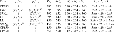
Simulation parameters for all cases: CP395, constant-property case with
 $Re_{\unicode[STIX]{x1D70F}}=395$
;
 $\text{C}Re_{\unicode[STIX]{x1D70F}}^{\star }$
, variable-property case with constant
 $Re_{\unicode[STIX]{x1D70F}}^{\star }$
(
 $=395$
) across the channel; GL, case with gas-like property variations;
 $\text{S}Re_{\unicode[STIX]{x1D70F}GL}^{\star }$
, variable-property case with
 $Re_{\unicode[STIX]{x1D70F}}^{\star }$
similar to case GL; LL, case with liquid-like property variations;
 $\text{S}Re_{\unicode[STIX]{x1D70F}LL}^{\star }$
, variable-property case with
 $Re_{\unicode[STIX]{x1D70F}}^{\star }$
similar to case LL; CP150, constant-property case with
 $Re_{\unicode[STIX]{x1D70F}}=150$
; CP550, constant-property case with
 $Re_{\unicode[STIX]{x1D70F}}=550$
.

Eight cases have been simulated, which are summarised in table 1. The simulations consist of three constant-property (CP395, CP150, CP550) and five variable-property cases (
 $\text{C}Re_{\unicode[STIX]{x1D70F}}^{\star }$
,
 $\text{S}Re_{\unicode[STIX]{x1D70F}GL}^{\star }$
, GL, LL,
 $\text{S}Re_{\unicode[STIX]{x1D70F}LL}^{\star }$
). The acronym CP refers to a constant-property case; GL and LL refer to gas-like and liquid-like property variations respectively;
 $\text{C}Re_{\unicode[STIX]{x1D70F}}^{\star }$
refers to a variable-property case with constant
 $Re_{\unicode[STIX]{x1D70F}}^{\star }$
(
 $=395$
) across the whole channel;
 $\text{S}Re_{\unicode[STIX]{x1D70F}GL}^{\star }$
refers to a variable-property case that has a similar
 $Re_{\unicode[STIX]{x1D70F}}^{\star }$
distribution to case GL; and
 $\text{S}Re_{\unicode[STIX]{x1D70F}LL}^{\star }$
refers to a variable-property case with an
 $Re_{\unicode[STIX]{x1D70F}}^{\star }$
distribution similar to case LL. The second and third columns show the functional relations for
 $\unicode[STIX]{x1D70C}/\unicode[STIX]{x1D70C}_{w}$
and
 $\unicode[STIX]{x1D707}/\unicode[STIX]{x1D707}_{w}$
as a function of
 $T/T_{w}$
. The next two columns report the wall-based friction Reynolds number
 $Re_{\unicode[STIX]{x1D70F}}$
and the semilocal Reynolds number at the channel centre
 ${Re_{\unicode[STIX]{x1D70F}}^{\star }}_{c}=Re_{\unicode[STIX]{x1D70F}}\sqrt{(\overline{\unicode[STIX]{x1D70C}}_{c}/\overline{\unicode[STIX]{x1D70C}}_{w})}/(\overline{\unicode[STIX]{x1D707}}_{c}/\overline{\unicode[STIX]{x1D707}}_{w})$
(the subscript
 $c$
denotes the value at the channel centre). It should be noted that at the wall
 ${Re_{\unicode[STIX]{x1D70F}}^{\star }}_{w}=Re_{\unicode[STIX]{x1D70F}}$
. The last two columns show the number of mesh points
 $N$
and the length of the domain
 $L$
along the streamwise
 $x$
, wall-normal
 $y$
and spanwise
 $z$
directions. The velocity components along the
 $x$
,
 $y$
and
 $z$
directions are denoted as
 $u$
,
 $v$
and
 $w$
respectively.
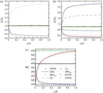
(a) Density
 $\overline{\unicode[STIX]{x1D70C}}/\overline{\unicode[STIX]{x1D70C}}_{w}$
, (b) viscosity
 $\overline{\unicode[STIX]{x1D707}}/\overline{\unicode[STIX]{x1D707}}_{w}$
and (c) semilocal Reynolds number
 $Re_{\unicode[STIX]{x1D70F}}^{\star }$
.

Figure 1 shows the distributions of density, viscosity and
 $Re_{\unicode[STIX]{x1D70F}}^{\star }$
for all cases. Cases with variable density are shown as lines and cases with constant density are shown as symbols. As can be seen, we use different combinations of
 $\unicode[STIX]{x1D70C}$
and
 $\unicode[STIX]{x1D707}$
to obtain quasisimilar
 $Re_{\unicode[STIX]{x1D70F}}^{\star }$
profiles. It should be noted that the strongest gradients in
 $Re_{\unicode[STIX]{x1D70F}}^{\star }$
occur at the wall. The cases forming the first pair – CP395 and
 $\text{C}Re_{\unicode[STIX]{x1D70F}}^{\star }$
(black symbols and line respectively, colour online) – have constant
 $Re_{\unicode[STIX]{x1D70F}}^{\star }$
in the wall-normal direction (
 $\text{d}Re_{\unicode[STIX]{x1D70F}}^{\star }/\text{d}y=0$
), even though for case
 $\text{C}Re_{\unicode[STIX]{x1D70F}}^{\star }$
the density and viscosity are varying and decrease away from the wall. For the second pair –
 $\text{S}Re_{\unicode[STIX]{x1D70F}GL}^{\star }$
and GL (blue symbols and line respectively, colour online) – the profile for
 $Re_{\unicode[STIX]{x1D70F}}^{\star }$
decreases from 395 at the wall to approximately 150 at the channel centre. Later, we will denote these cases as
 $\text{d}Re_{\unicode[STIX]{x1D70F}}^{\star }/\text{d}y<0$
. For the pair
 $LL$
and
 $\text{S}Re_{\unicode[STIX]{x1D70F}LL}^{\star }$
(red symbols and line respectively, colour online),
 $Re_{\unicode[STIX]{x1D70F}}^{\star }$
increases from 150 at the wall to approximately 540 at the channel centre. These cases will be denoted as
 $\text{d}Re_{\unicode[STIX]{x1D70F}}^{\star }/\text{d}y>0$
. The simulations CP150 (brown symbol, colour online) and CP550 (green symbol, colour online) are cases that bound the
 $Re_{\unicode[STIX]{x1D70F}}^{\star }$
profiles of the variable-property cases in order to investigate and distinguish any Reynolds-number effects with respect to effects caused by property gradients. Considerable variations in properties have been obtained for all variable-property cases. However, the relative property fluctuations
 ${\unicode[STIX]{x1D70C}^{\prime }}_{rms}/\overline{\unicode[STIX]{x1D70C}}$
and
 ${\unicode[STIX]{x1D707}^{\prime }}_{rms}/\overline{\unicode[STIX]{x1D707}}$
(the prime denotes Reynolds average fluctuations, and the subscript rms indicates the root-mean-square value) are still less than 0.15 for all variable-property cases.
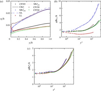
Kolmogorov length scale normalised by and plotted using (a) outer scales, (b) wall-based viscous length scales and (c) semilocal viscous length scales.

The adequacy of the mesh resolution to resolve the smallest scales is evaluated by means of wall-normal distributions of Kolmogorov length scales,
 $\unicode[STIX]{x1D702}=((\overline{\unicode[STIX]{x1D707}}/\overline{\unicode[STIX]{x1D70C}})^{3}\overline{\unicode[STIX]{x1D70C}}/\unicode[STIX]{x1D716})^{0.25}$
(
 $\unicode[STIX]{x1D716}$
is the turbulent kinetic energy dissipation per unit volume). Figure 2 shows
 $\unicode[STIX]{x1D702}$
, normalised by and plotted using outer scales (figure 2
a), wall-based viscous length scales (figure 2
b) and semilocal viscous length scales (figure 2
c) for all cases. Cases with similar
 $Re_{\unicode[STIX]{x1D70F}}^{\star }$
profiles show similar distributions of Kolmogorov scales, indicating that, similarly to turbulence statistics (Patel et al.
Reference Patel, Peeters, Boersma and Pecnik2015), the smallest scales are also strongly governed by
 $Re_{\unicode[STIX]{x1D70F}}^{\star }$
. The Kolmogorov scale normalised using the half-channel height increases for cases with decreasing
 $Re_{\unicode[STIX]{x1D70F}}^{\star }$
, while it decreases for cases with increasing
 $Re_{\unicode[STIX]{x1D70F}}^{\star }$
. The cases with
 $\text{d}Re_{\unicode[STIX]{x1D70F}}^{\star }/\text{d}y<0$
, for which
 $Re_{\unicode[STIX]{x1D70F}}^{\star }$
varies from 395 at the wall to approximately 140 at the channel centre, have a Kolmogorov length scale that transitions from the values of case CP395 at the wall to CP150 at the channel centre. A similar observation can be made for cases with
 $\text{d}Re_{\unicode[STIX]{x1D70F}}^{\star }/\text{d}y>0$
, for which
 $Re_{\unicode[STIX]{x1D70F}}^{\star }$
varies from 150 at the wall to approximately 540 at the centre. The Kolmogorov scale, when normalised by and plotted using classical wall-based viscous units, shows strong deviations for cases with
 $\text{d}Re_{\unicode[STIX]{x1D70F}}^{\star }/\text{d}y\neq 0$
. On the other hand, the use of semilocal length scales provides a good collapse of
 $\unicode[STIX]{x1D702}$
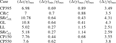
for all cases in the near-wall region. Hence, the semilocal scaling also provides a good measure to assess the mesh spacing requirements for simulations with strong fluid property variations. Table 2 lists the maximum grid spacing in terms of
 $\unicode[STIX]{x1D702}$
for all cases, and the values are within the resolution requirements of
 $\unicode[STIX]{x0394}x<12\unicode[STIX]{x1D702}$
,
 $\unicode[STIX]{x0394}y<2\unicode[STIX]{x1D702}$
,
 $\unicode[STIX]{x0394}z<6\unicode[STIX]{x1D702}$
, as also reported in other DNS studies (Zonta et al.
Reference Zonta, Marchioli and Soldati2012; Lee et al.
Reference Lee, Yoon Jung, Jin Sung and Zaki2013).
Maximum spatial resolution normalised using the Kolmogorov scale
 $\unicode[STIX]{x1D702}$
.

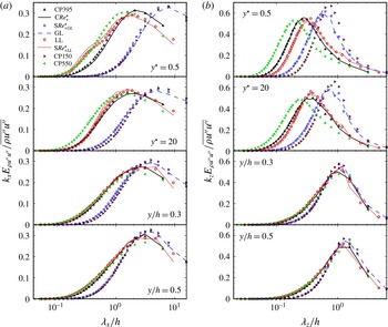
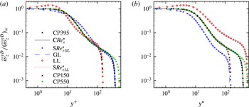
The adequacy of the box size to accommodate the large-scale structures can be studied using the one-dimensional premultiplied energy spectrum, defined as
 $$\begin{eqnarray}\unicode[STIX]{x1D719}_{\unicode[STIX]{x1D70C}u^{\prime \prime }u^{\prime \prime }}(k_{\unicode[STIX]{x1D6FC}})=k_{\unicode[STIX]{x1D6FC}}[{\mathcal{F}}(\sqrt{\unicode[STIX]{x1D70C}}u^{\prime \prime }){\mathcal{F}}(\sqrt{\unicode[STIX]{x1D70C}}u^{\prime \prime })^{\ast }]=k_{\unicode[STIX]{x1D6FC}}[E_{\unicode[STIX]{x1D70C}u^{\prime \prime }u^{\prime \prime }}(k_{\unicode[STIX]{x1D6FC}})].\end{eqnarray}$$
In the above equation,
 ${\mathcal{F}}(\unicode[STIX]{x1D713})$
is the Fourier coefficient of
 $\unicode[STIX]{x1D713}$
,
 ${\mathcal{F}}(\unicode[STIX]{x1D713})^{\ast }$
is the complex conjugate,
 $E_{\unicode[STIX]{x1D70C}u^{\prime \prime }u^{\prime \prime }}={\mathcal{F}}(\sqrt{\unicode[STIX]{x1D70C}}u^{\prime \prime }){\mathcal{F}}(\sqrt{\unicode[STIX]{x1D70C}}u^{\prime \prime })^{\ast }$
represents the energy spectrum of the density-weighted streamwise velocity fluctuation, the double prime denotes Favre-averaged fluctuations and
 $k_{\unicode[STIX]{x1D6FC}}$
is the wavenumber in the streamwise
 $k_{x}$
or spanwise
 $k_{z}$
direction. The streamwise Reynolds stress is related to
 $\unicode[STIX]{x1D719}_{\unicode[STIX]{x1D70C}u^{\prime \prime }u^{\prime \prime }}$
and
 $E_{\unicode[STIX]{x1D70C}u^{\prime \prime }u^{\prime \prime }}$
as
 $$\begin{eqnarray}\overline{\unicode[STIX]{x1D70C}u^{\prime \prime }u^{\prime \prime }}=\overline{\unicode[STIX]{x1D70C}}\widetilde{u^{\prime \prime }u^{\prime \prime }}=\int _{0}^{\infty }E_{\unicode[STIX]{x1D70C}u^{\prime \prime }u^{\prime \prime }}(k_{\unicode[STIX]{x1D6FC}})\,\text{d}k_{\unicode[STIX]{x1D6FC}}=\int _{0}^{\infty }\unicode[STIX]{x1D719}_{\unicode[STIX]{x1D70C}u^{\prime \prime }u^{\prime \prime }}(k_{\unicode[STIX]{x1D6FC}})\,\text{d}(\log \unicode[STIX]{x1D706}_{\unicode[STIX]{x1D6FC}}),\end{eqnarray}$$
where the tilde denotes Favre averaging and
 $\unicode[STIX]{x1D706}_{\unicode[STIX]{x1D6FC}}=2\unicode[STIX]{x03C0}/k_{\unicode[STIX]{x1D6FC}}$
is the wavelength. The area under the premultiplied spectrum, when plotted in lin-log scale, represents the Reynolds stress. A plot of
 $\unicode[STIX]{x1D719}_{\unicode[STIX]{x1D70C}u^{\prime \prime }u^{\prime \prime }}$
, normalised by
 $\overline{\unicode[STIX]{x1D70C}u^{\prime \prime }u^{\prime \prime }}$
and plotted as a function of streamwise and spanwise wavelength at different wall-normal planes, is shown in figure 3. While the spanwise spectrum indicates that the spanwise box size is sufficient, it can be argued that the length of the box in the streamwise direction could be increased to resolve all of the large-scale contributions. However, as noted in previous studies (Abe, Kawamura & Choi Reference Abe, Kawamura and Choi2004; Lozano-Durán & Jiménez Reference Lozano-Durán and Jiménez2014), the influence of these unresolved large-scale structures (due to the moderate box size) on turbulence statistics is negligible, and resolving the peak of the streamwise premultiplied spectrum (e.g. DNS data of Moser, Kim & Mansour (Reference Moser, Kim and Mansour1999)) was considered sufficient for the present work. The spanwise premultiplied spectrum
 $\unicode[STIX]{x1D719}_{\unicode[STIX]{x1D70C}u^{\prime \prime }u^{\prime \prime }}(k_{z})$
will be discussed in more detail in § 5 to highlight its scaling characteristics.
(a) Normalised premultiplied streamwise spectrum
 $k_{x}E_{\unicode[STIX]{x1D70C}u^{\prime \prime }u^{\prime \prime }}/\overline{\unicode[STIX]{x1D70C}u^{\prime \prime }u^{\prime \prime }}$
as a function of streamwise wavelength
 $\unicode[STIX]{x1D706}_{x}/h$
and (b) normalised premultiplied spanwise spectrum
 $k_{z}E_{\unicode[STIX]{x1D70C}u^{\prime \prime }u^{\prime \prime }}/\overline{\unicode[STIX]{x1D70C}u^{\prime \prime }u^{\prime \prime }}$
as a function of spanwise wavelength
 $\unicode[STIX]{x1D706}_{z}/h$
, at different wall-normal locations.

3 Mean velocity scaling
This section discusses the effect of near-wall gradients in density and viscosity on the scaling of mean velocity profiles. We first highlight shortcomings of the van Driest transformation for cases with strong near-wall gradients in
 $Re_{\unicode[STIX]{x1D70F}}^{\star }$
. We then derive a semilocally scaled stress-balance equation and show that the viscous stresses for the investigated cases perfectly collapse, if they are plotted as a function of the semilocal wall distance
 $y^{\star }$
. We will utilise this collapse to derive a velocity scaling that will be applied for the turbulent channel flows discussed above, and for adiabatic supersonic turbulent boundary layers.
The van Driest transformed velocity
 $\overline{u}^{vD}$
and the diagnostic function
 $y\,\text{d}\overline{u}^{vD}/\text{d}y$
as a function of
 $y^{+}$
and
 $y^{\star }$
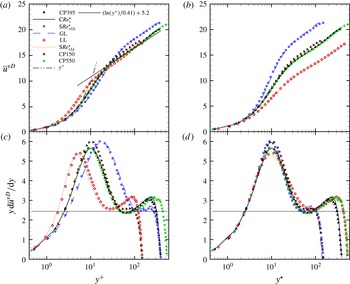
for all cases are shown in figure 4. As noted in our earlier study, cases with quasisimilar
 $Re_{\unicode[STIX]{x1D70F}}^{\star }$
profiles (symbols and lines with the same colour online) exhibit similar
 $\overline{u}^{vD}$
profiles, irrespective of their individual density and viscosity profiles. However, when comparing cases with different
 $Re_{\unicode[STIX]{x1D70F}}^{\star }$
gradients, deviations can be observed. For example, in figure 4(a), the slope of the linear viscous sublayer (
 $\overline{u}^{vD}=y^{+}$
) increases for cases with
 $\text{d}Re_{\unicode[STIX]{x1D70F}}^{\star }/\text{d}y>0$
(red line and symbols, colour online) and decreases for cases with
 $\text{d}Re_{\unicode[STIX]{x1D70F}}^{\star }/\text{d}y<0$
(blue line and symbols, colour online). Moreover, an increase in the log-law additive constant (commonly
 $B=5.2$
) can be seen for cases with
 $\text{d}Re_{\unicode[STIX]{x1D70F}}^{\star }/\text{d}y<0$
, while the opposite is observed for cases with
 $\text{d}Re_{\unicode[STIX]{x1D70F}}^{\star }/\text{d}y>0$
. Additionally, the log-layer shifts outwards for cases with
 $\text{d}Re_{\unicode[STIX]{x1D70F}}^{\star }/\text{d}y<0$
and inwards for cases with
 $\text{d}Re_{\unicode[STIX]{x1D70F}}^{\star }/\text{d}y>0$
, as can be seen from the profiles of the diagnostic function
 $y\,\text{d}\overline{u}^{vD}/\text{d}y$
in figure 4(c). Figure 4(b,d) shows
 $\overline{u}^{vD}$
and the diagnostic function for all cases as a function of
 $y^{\star }$
. The deviation of
 $\overline{u}^{vD}$
for cases with
 $\text{d}Re_{\unicode[STIX]{x1D70F}}^{\star }/\text{d}y\neq 0$
is even more prominent if plotted as a function of
 $y^{\star }$
. On the other hand, the diagnostic function collapses the onset of the log-layer if plotted as a function of
 $y^{\star }$
. The reason for this collapse is investigated further using the streamwise stress-balance equation.
(a,b) van Driest velocity
 $\overline{u}^{vD}$
and (c,d) diagnostic function
 $y\,\text{d}\overline{u}^{vD}/\text{d}y$
shown as a function of
 $y^{+}$
(a,c) and
 $y^{\star }$
(b,d). The solid horizontal line in (c) and (d) has a value of
 $1/0.41$
.

The stress-balance relation for the turbulent and viscous stresses can be obtained by integrating the mean streamwise momentum equation, which, for a fully developed turbulent channel flow (neglecting viscosity fluctuations), gives
 $$\begin{eqnarray}-\frac{\overline{\unicode[STIX]{x1D70C}}\widetilde{u^{\prime \prime }v^{\prime \prime }}}{\overline{\unicode[STIX]{x1D70C}}_{w}u_{\unicode[STIX]{x1D70F}}^{2}}+\frac{h}{Re_{\unicode[STIX]{x1D70F}}}\left(\frac{\overline{\unicode[STIX]{x1D707}}}{\overline{\unicode[STIX]{x1D707}}_{w}}\right)\frac{\text{d}(\overline{u}/u_{\unicode[STIX]{x1D70F}})}{\text{d}y}\approx \frac{\unicode[STIX]{x1D70F}}{\unicode[STIX]{x1D70F}_{w}}=\left(1-\frac{y}{h}\right),\end{eqnarray}$$
where
 $\unicode[STIX]{x1D70F}$
and
 $\unicode[STIX]{x1D70F}_{w}$
are the total and wall shear stress respectively. Analogously to Patel et al. (Reference Patel, Peeters, Boersma and Pecnik2015), equation (3.1) can be written in terms of semilocally scaled velocity fluctuations (using the semilocal friction velocity
 $u_{\unicode[STIX]{x1D70F}}^{\star }=\sqrt{\unicode[STIX]{x1D70F}_{w}/\overline{\unicode[STIX]{x1D70C}}}$
)
 $$\begin{eqnarray}\hat{u} _{i}^{\prime }\approx \frac{u_{i}^{\prime \prime }}{u_{\unicode[STIX]{x1D70F}}^{\star }}=\sqrt{\frac{\overline{\unicode[STIX]{x1D70C}}}{\overline{\unicode[STIX]{x1D70C}}_{w}}}\left(\frac{u_{i}^{\prime \prime }}{u_{\unicode[STIX]{x1D70F}}}\right)\end{eqnarray}$$
and the van Driest mean velocity increment
 $$\begin{eqnarray}\text{d}\overline{u}^{vD}=\sqrt{\frac{\overline{\unicode[STIX]{x1D70C}}}{\overline{\unicode[STIX]{x1D70C}}_{w}}}\text{d}\left(\frac{\overline{u}}{u_{\unicode[STIX]{x1D70F}}}\right),\end{eqnarray}$$
to obtain the semilocally scaled stress-balance equation
 $$\begin{eqnarray}-\widetilde{\hat{u} ^{\prime }\hat{v}^{\prime }}+\frac{h}{Re_{\unicode[STIX]{x1D70F}}^{\star }}\frac{\text{d}\overline{u}^{vD}}{\text{d}y}\approx \frac{\unicode[STIX]{x1D70F}}{\unicode[STIX]{x1D70F}_{w}}=\left(1-\frac{y}{h}\right).\end{eqnarray}$$
It should be noted that the viscous stress term is a function of the van Driest mean velocity gradient, scaled by the inverse of the semilocal Reynolds number. The reason for writing (3.1) in terms of
 $\overline{u}^{vD}$
and
 $\widetilde{\hat{u} ^{\prime }\hat{v}^{\prime }}$
originates from Patel et al. (Reference Patel, Peeters, Boersma and Pecnik2015), where the Navier–Stokes equations were rescaled using the semilocal friction velocity and local mean properties in order to obtain governing equations for the semilocally scaled mean,
 $\overline{u}^{vD}$
, and fluctuating velocities,
 $\hat{u} _{i}^{\prime }$
, with
 $Re_{\unicode[STIX]{x1D70F}}^{\star }$
as a strong parameter. In other words, the combined influence of density and viscosity variations on turbulence statistics can be characterised using a single parameter,
 $Re_{\unicode[STIX]{x1D70F}}^{\star }$
.
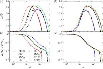
(a,b) Reynolds shear stress
 $-\widetilde{\hat{u} ^{\prime }\hat{v}^{\prime }}$
and (c,d) viscous shear stress
 $(h/Re_{\unicode[STIX]{x1D70F}}^{\star })\,\text{d}\overline{u}^{vD}/\text{d}y$
shown as a function of
 $y^{+}$
(a,c) and
 $y^{\star }$
(b,d).

The Reynolds shear stress
 $\widetilde{\hat{u} ^{\prime }\hat{v}^{\prime }}$
and viscous stress term
 $(h/Re_{\unicode[STIX]{x1D70F}}^{\star })\,\text{d}\overline{u}^{vD}/\text{d}y$
in (3.4) are plotted as a function of
 $y^{+}$
and
 $y^{\star }$
in figure 5. It is apparent that neither stress collapses if shown as a function of
 $y^{+}$
(figure 5
a,c) for cases with different
 $Re_{\unicode[STIX]{x1D70F}}^{\star }$
gradients. Similar observations have been reported for compressible non-adiabatic flows in Coleman et al. (Reference Coleman, Kim and Moser1995), Foysi et al. (Reference Foysi, Sarkar and Friedrich2004) and Morinishi et al. (Reference Morinishi, Tamano and Nakabayashi2004), and in Patel et al. (Reference Patel, Peeters, Boersma and Pecnik2015) for low-Mach-number channel flows with gradients in
 $Re_{\unicode[STIX]{x1D70F}}^{\star }$
. In comparison to a constant-property case with a similar
 $Re_{\unicode[STIX]{x1D70F}}$
value, the Reynolds shear stress decreases for cases with
 $\text{d}Re_{\unicode[STIX]{x1D70F}}^{\star }/\text{d}y<0$
and increases for cases with
 $\text{d}Re_{\unicode[STIX]{x1D70F}}^{\star }/\text{d}y>0$
. On the other hand, if the stresses are plotted as a function of
 $y^{\star }$
(figure 5
b,d), two observations can be made. First, the Reynolds shear stress profiles for all cases collapse closely in the inner layer, except in the region very close to the wall where small differences can be seen. Second, and more importantly, the viscous stresses for all cases perfectly collapse over the entire
 $y^{\star }$
range. Given the last observation, it is evident that the viscous stress term, expressed as
 $(h/Re_{\unicode[STIX]{x1D70F}}^{\star })\,\text{d}\overline{u}^{vD}/\,\text{d}y$
, forms the basis to develop a proper scaling law for the mean velocity in flows with large density and viscosity gradients. We thus propose that the transformation must be based on the viscous stress
 $$\begin{eqnarray}\frac{h}{Re_{\unicode[STIX]{x1D70F}}^{\star }}\frac{\text{d}\overline{u}^{vD}}{\text{d}y}=\unicode[STIX]{x1D6F7}(y^{\star }),\end{eqnarray}$$
where
 $\unicode[STIX]{x1D6F7}$
is an unknown function of
 $y^{\star }$
. Using the chain rule
 $\text{d}/\text{d}y=(\text{d}y^{\star }/\text{d}y)\,\text{d}/\text{d}y^{\star }$
, we can write (3.5) as
 $$\begin{eqnarray}\frac{h}{Re_{\unicode[STIX]{x1D70F}}^{\star }}\left(\frac{\text{d}y^{\star }}{\text{d}y}\right)\frac{\text{d}\overline{u}^{vD}}{\text{d}y^{\star }}=\unicode[STIX]{x1D6F7}(y^{\star }).\end{eqnarray}$$
This allows us to replace
 $\text{d}y^{\star }/\text{d}y$
in (3.6) by taking the derivative of
 $y^{\star }=yRe_{\unicode[STIX]{x1D70F}}^{\star }/h$
with respect to
 $y$
, to obtain
 $$\begin{eqnarray}\left(1+\frac{y}{Re_{\unicode[STIX]{x1D70F}}^{\star }}\frac{\text{d}Re_{\unicode[STIX]{x1D70F}}^{\star }}{\text{d}y}\right)\frac{\text{d}\overline{u}^{vD}}{\text{d}y^{\star }}=\unicode[STIX]{x1D6F7}(y^{\star }).\end{eqnarray}$$
Equation (3.7) thus provides the scaling law for the mean streamwise velocity, which we will denote as
 $\overline{u}^{\star }$
. Hence,
 $\text{d}\overline{u}^{\star }$
and
 $\text{d}\overline{u}^{vD}$
are related through
 $$\begin{eqnarray}\text{d}\overline{u}^{\star }=\left(1+\frac{y}{Re_{\unicode[STIX]{x1D70F}}^{\star }}\frac{\text{d}Re_{\unicode[STIX]{x1D70F}}^{\star }}{\text{d}y}\right)\text{d}\overline{u}^{vD}=\unicode[STIX]{x1D6F7}(y^{\star })\,\text{d}y^{\star }.\end{eqnarray}$$
It should be noted that the transformation proposed by Trettel & Larsson (Reference Trettel and Larsson2016) is equivalent when substituting the definitions of
 $Re_{\unicode[STIX]{x1D70F}}^{\star }$
and
 $d\overline{u}^{vD}$
into (3.8). Their transformation, which is expressed in terms of density and viscosity gradients, was obtained by equating the transformed log-law velocity gradient with the velocity gradient obtained from the stress-balance equation, assuming that the Reynolds shear stress is similar for compressible and constant-property cases. The present derivation follows an alternative route. It is based on rescaling the Navier–Stokes equations using the local mean properties and semilocal friction velocity, which naturally suggests that the viscous terms are scaled by the semilocal Reynolds number
 $Re_{\unicode[STIX]{x1D70F}}^{\star }$
to account for changes in viscous scales due to property variations. The transformation expressed in terms of (3.8) thus emphasises the fact that, similarly to turbulence statistics, the transformation is also governed by the
 $Re_{\unicode[STIX]{x1D70F}}^{\star }$
profiles, rather than individual density and viscosity profiles.
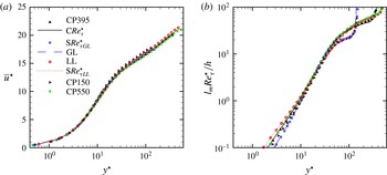
The derived velocity transformation
 $\overline{u}^{\star }=\int _{0}^{\overline{u}^{vD}}(1+(y/Re_{\unicode[STIX]{x1D70F}}^{\star })\text{d}Re_{\unicode[STIX]{x1D70F}}^{\star }/\text{d}y)\,\text{d}\overline{u}^{vD}$
, is shown in figure 6(a) as a function of
 $y^{\star }$
. It can be seen that
 $\overline{u}^{\star }$
is perfectly able to collapse the velocity profiles for all cases over the entire
 $y^{\star }$
range. In our previous work (Patel et al.
Reference Patel, Peeters, Boersma and Pecnik2015), we showed that similar turbulence statistics and van Driest mean velocity profiles
 $\overline{u}^{vD}$
are obtained for cases with similar
 $Re_{\unicode[STIX]{x1D70F}}^{\star }$
distributions, even if their individual mean density and viscosity profiles substantially differ. Here, we derive a transformation that accounts for gradients in
 $Re_{\unicode[STIX]{x1D70F}}^{\star }$
in order to extend the van Driest transformation.
Using the derived velocity transformation it is also possible to explain the collapse of the diagnostic function as a function of
 $y^{\star }$
, as mentioned earlier. The definitions in (3.5) and (3.8) can be expressed as
 $$\begin{eqnarray}\frac{h}{Re_{\unicode[STIX]{x1D70F}}^{\star }}\frac{\text{d}\overline{u}^{vD}}{\text{d}y}=\frac{\text{d}\overline{u}^{\star }}{\text{d}y^{\star }}=\unicode[STIX]{x1D6F7}(y^{\star }).\end{eqnarray}$$
By substituting
 $h/Re_{\unicode[STIX]{x1D70F}}^{\star }=y/y^{\star }$
in (3.9) we can obtain the correlation between the diagnostic function and the newly derived velocity scale
 $u^{\star }$
as
 $$\begin{eqnarray}y\frac{\text{d}\overline{u}^{vD}}{\text{d}y}=y^{\star }\frac{\text{d}\overline{u}^{\star }}{\text{d}y^{\star }}=y^{\star }\unicode[STIX]{x1D6F7}(y^{\star }),\end{eqnarray}$$
which explains the collapse of the diagnostic function in figure 4(d).
(a) Transformed velocity
 $\overline{u}^{\star }$
and (b) mixing length
 $l_{m}Re_{\unicode[STIX]{x1D70F}}^{\star }/h$
as a function of
 $y^{\star }$
.

The invariance of
 $\unicode[STIX]{x1D6F7}$
as a function of
 $y^{\star }$
can be further quantified by expressing it in terms of the turbulence mixing length. Following Huang & Coleman (Reference Huang and Coleman1994), the Reynolds shear stress can be written in terms of the velocity gradient using the mixing-length theory as
 $$\begin{eqnarray}l_{m}^{2}=\frac{-\widetilde{u^{\prime \prime }v^{\prime \prime }}}{(\text{d}\overline{u}/\text{d}y)^{2}}=\frac{-\widetilde{\hat{u} ^{\prime }\hat{v}^{\prime }}}{(\text{d}\overline{u}^{vD}/\text{d}y)^{2}}.\end{eqnarray}$$
Substitution of the Reynolds shear stress in (3.4) using (3.11) results in a quadratic equation for
 $\text{d}\overline{u}^{vD}/\text{d}y$
, which, when solved and simplified, gives
 $$\begin{eqnarray}\unicode[STIX]{x1D6F7}(y^{\star })=\frac{2\unicode[STIX]{x1D70F}/\unicode[STIX]{x1D70F}_{w}}{1+\sqrt{1+4\unicode[STIX]{x1D70F}/\unicode[STIX]{x1D70F}_{w}(l_{m}Re_{\unicode[STIX]{x1D70F}}^{\star }/h)^{2}}}.\end{eqnarray}$$
The above expression naturally suggests that
 $l_{m}$
scales with the semilocal length scale
 $h/Re_{\unicode[STIX]{x1D70F}}^{\star }$
. Figure 6(b) shows
 $l_{m}Re_{\unicode[STIX]{x1D70F}}^{\star }/h$
as a function of
 $y^{\star }$
. A satisfactory collapse is obtained for almost the entire inner layer, except very close to wall where small deviations occur. These deviations stem from turbulence modulation caused by strong
 $Re_{\unicode[STIX]{x1D70F}}^{\star }$
gradients, which we will discuss in detail in §§ 4 and 5. However, close to the wall the viscous stress dominates and small values of the mixing length do not alter the velocity scaling.
(a) The
 $Re_{\unicode[STIX]{x1D70F}}^{\star }$
distribution shown as a function of
 $y^{\star }$
, (b) the van Driest velocity
 $\overline{u}^{vD}$
shown as a function of
 $y^{+}$
and (c) the transformed velocity
 $\overline{u}^{\star }$
shown as a function of
 $y^{\star }$
for adiabatic supersonic boundary layers obtained from Bernardini & Pirozzoli (Reference Bernardini and Pirozzoli2011) and Pirozzoli & Bernardini (Reference Pirozzoli and Bernardini2011), compared with reference boundary layer data from Jiménez et al. (Reference Jiménez, Hoyas, Simens and Mizuno2010).

(a,b) Reynolds shear stress
 $-\widetilde{\hat{u} ^{\prime }\hat{v}^{\prime }}$
and (c,d) viscous shear stress
 $(h/Re_{\unicode[STIX]{x1D70F}}^{\star })\,\text{d}\overline{u}^{vD}/\text{d}y$
shown as a function of
 $y^{+}$
(a,c) and
 $y^{\star }$
(b,d) for adiabatic supersonic boundary layers obtained from Bernardini & Pirozzoli (Reference Bernardini and Pirozzoli2011) and Pirozzoli & Bernardini (Reference Pirozzoli and Bernardini2011), compared with boundary layer data from Jiménez et al. (Reference Jiménez, Hoyas, Simens and Mizuno2010).

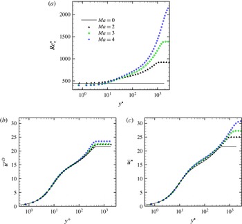
In the following, we will investigate whether the scaling can also be successfully applied for supersonic adiabatic flows, for which the van Driest scaling already shows a satisfying collapse. For this we will use a DNS database for adiabatic supersonic boundary layers from Bernardini & Pirozzoli (Reference Bernardini and Pirozzoli2011) and Pirozzoli & Bernardini (Reference Pirozzoli and Bernardini2011), and data for an incompressible boundary layer from Jiménez et al. (Reference Jiménez, Hoyas, Simens and Mizuno2010). The investigated compressible cases have Mach numbers of
 $Ma=2$
, 3 and 4 and corresponding Reynolds numbers of
 $Re_{\unicode[STIX]{x1D70F}}=450$
, 400 and 400 respectively. The incompressible boundary layer is at
 $Re_{\unicode[STIX]{x1D70F}}=450$
. Figure 7(a) shows the
 $Re_{\unicode[STIX]{x1D70F}}^{\star }$
distribution for these cases as a function of
 $y^{\star }$
. It should be noted that, in contrast to the heated and cooled channel flows, the gradient of
 $Re_{\unicode[STIX]{x1D70F}}^{\star }$
at the wall is negligible. The largest
 $Re_{\unicode[STIX]{x1D70F}}^{\star }$
variation is obtained for the
 $Ma=4$
case, where
 $Re_{\unicode[STIX]{x1D70F}}^{\star }$
at the edge of the boundary layer is more than four times larger than at the wall. The van Driest mean velocity
 $\overline{u}^{vD}$
is plotted as a function of
 $y^{+}$
in figure 7(b). A satisfying collapse for the compressible and incompressible boundary layers is obtained, except in the wake region, which has been studied in more detail by Zhang et al. (Reference Zhang, Bi, Hussain, Li and She2012). The transformed velocity
 $\overline{u}^{\star }$
as a function of
 $y^{\star }$
is shown in figure 7(c). Here also, a reasonable collapse for the
 $\overline{u}^{\star }$
velocity profiles is obtained. However, small deviations with respect to the incompressible boundary layer occur in the buffer and logarithmic regions. Interestingly, Trettel & Larsson (Reference Trettel and Larsson2016) have also found a similar disagreement for cooled turbulent boundary layers.
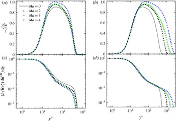
The implication of the above mean velocity scaling characteristics on the stress-balance relation for these turbulent boundary layers is discussed next. The Reynolds shear and viscous stresses are shown in figure 8 as a function of
 $y^{+}$
and
 $y^{\star }$
. Both stresses show a superior collapse if they are plotted as a function of
 $y^{\star }$
. Analogously to the plot of
 $\overline{u}^{\star }$
versus
 $y^{\star }$
in figure 7(c), the viscous stresses of the compressible cases also deviate slightly from the incompressible case, as can be seen in figure 8(d). On the other hand, if the stresses are plotted as a function of
 $y^{+}$
, it can be seen that the turbulent shear stress profiles increase and the viscous stress profiles decrease with Mach number; see figure 8(a,c). This Mach number dependence of the stresses as a function of
 $y^{+}$
can be shown mathematically by writing the stress-balance equation (3.4) for the incompressible and compressible boundary layers as
 $$\begin{eqnarray}\displaystyle & \displaystyle \left.\left(\widetilde{\hat{u} ^{\prime }\hat{v}^{\prime }}+\frac{\unicode[STIX]{x1D70F}}{\unicode[STIX]{x1D70F}_{w}}\right)\right|_{incomp}=\left.\frac{h}{Re_{\unicode[STIX]{x1D70F}}}\frac{\text{d}\overline{u}^{vD}}{\text{d}y}\right|_{incomp}\quad \text{for the incompressible BL}, & \displaystyle\end{eqnarray}$$
 $$\begin{eqnarray}\displaystyle & \displaystyle \left.\frac{Re_{\unicode[STIX]{x1D70F}}^{\star }}{Re_{\unicode[STIX]{x1D70F}}}\left(\widetilde{\hat{u} ^{\prime }\hat{v}^{\prime }}+\frac{\unicode[STIX]{x1D70F}}{\unicode[STIX]{x1D70F}_{w}}\right)\right|_{comp}=\left.\frac{h}{Re_{\unicode[STIX]{x1D70F}}}\frac{\text{d}\overline{u}^{vD}}{\text{d}y}\right|_{comp}\quad \text{for the compressible BL}. & \displaystyle\end{eqnarray}$$
In the constant-stress layer,
 $(\unicode[STIX]{x1D70F}/\unicode[STIX]{x1D70F}_{w})_{comp}=(\unicode[STIX]{x1D70F}/\unicode[STIX]{x1D70F}_{w})_{incomp}=1$
, and due to the collapse of
 $\overline{u}^{vD}$
as a function of
 $y^{+}$
, equations (3.13) and (3.14) can be equated as
 $$\begin{eqnarray}(\widetilde{\hat{u} ^{\prime }\hat{v}^{\prime }}+1)|_{incomp}=\left.\frac{Re_{\unicode[STIX]{x1D70F}}^{\star }}{Re_{\unicode[STIX]{x1D70F}}}(\widetilde{\hat{u} ^{\prime }\hat{v}^{\prime }}+1)\right|_{comp}.\end{eqnarray}$$
Therefore, if
 $Re_{\unicode[STIX]{x1D70F}}^{\star }>Re_{\unicode[STIX]{x1D70F}}$
, it follows that
 $(-\widetilde{\hat{u} ^{\prime }\hat{v}^{\prime }})|_{comp}>(-\widetilde{\hat{u} ^{\prime }\hat{v}^{\prime }})|_{incomp}$
, which explains the Mach number dependence of the stresses. The increase in shear stress for the supersonic cases also explains the corresponding increase in turbulence intensities when compared with incompressible cases (Pirozzoli, Grasso & Gatski Reference Pirozzoli, Grasso and Gatski2004; Bernardini & Pirozzoli Reference Bernardini and Pirozzoli2011), due to the increase in the turbulent kinetic energy production. The partial success of both
 $y^{+}$
and
 $y^{\star }$
in adiabatic supersonic boundary layers thus warrants future studies. The semilocal scaling utilises the invariance of
 $(h/Re_{\unicode[STIX]{x1D70F}}^{\star })\text{d}\overline{u}^{vD}/\text{d}y$
as a function of
 $y^{\star }$
to obtain
 $\overline{u}^{\star }$
, while adiabatic boundary layers exhibit invariance of a more fundamental variable, namely the wall-normalised van Driest transformed mean spanwise vorticity
 $\overline{\unicode[STIX]{x1D714}}_{z}^{vD}/(\overline{\unicode[STIX]{x1D714}}_{z}^{vD})_{w}=\text{d}\overline{u}^{vD}/\text{d}y^{+}=(h/Re_{\unicode[STIX]{x1D70F}})\text{d}\overline{u}^{vD}/\text{d}y$
, as a function of
 $y^{+}$
. More discussion on the significance of mean vorticity is provided in the next section.
4 Influence of
 $Re_{\unicode[STIX]{x1D70F}}^{\star }$
gradients on near-wall turbulence statistics

Turbulence statistics are strongly influenced by near-wall modifications of turbulence. Near-wall turbulence modifications for variable-property flows can be classified into two main mechanisms: (i) changes in viscous scales and (ii) structural changes of turbulence. The semilocal scaling is successful in collapsing turbulence statistics, such as mean velocity (see figure 6 a), Reynolds and viscous shear stress (see figure 5 b,d), because it accommodates the change in viscous scales using local quantities, and because these quantities are not significantly affected by structural changes and non-local effects very close to the wall. On the other hand, the semilocal scaling fails for turbulence statistics that are sensitive to strong non-local interactions of the buffer layer vortical structures with the sublayer region, e.g. statistics of vorticity fluctuations. Furthermore, the semilocal scaling also fails for turbulence statistics that contain direct information on turbulence structure, e.g. turbulence anisotropy (Foysi et al. Reference Foysi, Sarkar and Friedrich2004) and low-speed streaks (Patel et al. Reference Patel, Peeters, Boersma and Pecnik2015).
We first study the gradient of the van Driest transformed mean velocity
 $\overline{u}^{vD}$
, which we will refer to as the van Driest transformed mean spanwise vorticity
 $\overline{\unicode[STIX]{x1D714}}_{z}^{vD}$
. The van Driest transformed mean velocity
 $\overline{u}^{vD}$
is the analogue to the mean velocity in a variable-density flow, and therefore a study of its gradients allows us to draw conclusions on the stability of the flow. We then discuss the turbulent vorticity fluctuations and the turbulence anisotropy to emphasise the failure of the semilocal scaling due to non-locality and changes in turbulence structure respectively.
Wall-normalised van Driest transformed mean spanwise vorticity
 $\overline{\unicode[STIX]{x1D714}}_{z}^{vD}/(\overline{\unicode[STIX]{x1D714}}_{z}^{vD})_{w}$
shown as a function of (a)
 $y^{+}$
and (b)
 $y^{\star }$
.

4.1 Mean spanwise vorticity
The wall-normalised van Driest transformed mean spanwise vorticity
 $\overline{\unicode[STIX]{x1D714}}_{z}^{vD}/(\overline{\unicode[STIX]{x1D714}}_{z}^{vD})_{w}=\text{d}\overline{u}^{vD}/\text{d}y^{+}=(h/Re_{\unicode[STIX]{x1D70F}})\text{d}\overline{u}^{vD}/\text{d}y$
is plotted as a function of
 $y^{+}$
and
 $y^{\star }$
in figures 9(a) and 9(b) respectively. Unlike for adiabatic walls, where
 $\overline{\unicode[STIX]{x1D714}}_{z}^{vD}/(\overline{\unicode[STIX]{x1D714}}_{z}^{vD})_{w}$
is invariant as a function of
 $y^{+}$
in the inner layer (e.g. Pirozzoli & Bernardini Reference Pirozzoli and Bernardini2011),
 $\overline{\unicode[STIX]{x1D714}}_{z}^{vD}/(\overline{\unicode[STIX]{x1D714}}_{z}^{vD})_{w}$
is neither a function of
 $y^{+}$
nor
 $y^{\star }$
for non-adiabatic walls. Based on Eyink (Reference Eyink2008), vorticity generated at the wall is transported outward, first diffused by viscosity and subsequently advected by turbulence. Strong gradients in viscosity in the viscous-dominated region thus change the vorticity transport and consequently the mean velocity profile. The change in mean velocity profile then directly influences the turbulence. Equivalently, in variable-density flows, strong gradients in
 $Re_{\unicode[STIX]{x1D70F}}^{\star }$
(since
 $Re_{\unicode[STIX]{x1D70F}}^{\star }$
characterises the viscous scale) influence the van Driest transformed mean velocity profile. It is clearly visible in figure 9 that
 $\overline{\unicode[STIX]{x1D714}}_{z}^{vD}/(\overline{\unicode[STIX]{x1D714}}_{z}^{vD})_{w}$
shows a local maximum for cases with
 $\text{d}Re_{\unicode[STIX]{x1D70F}}^{\star }/\text{d}y>0$
(red line and symbols, colour online). This maximum implies an inflection point in the velocity profile, which also indicates a more unstable flow condition. The reverse happens for cases with
 $\text{d}Re_{\unicode[STIX]{x1D70F}}^{\star }/\text{d}y<0$
(blue line and symbols, colour online), where the velocity profile becomes fuller (higher negative curvature of
 $\text{d}^{2}\overline{u}^{vD}/\text{d}y^{2}$
), causing the flow to become more stable (Gad-el Hak Reference Gad-el Hak1990). This effect is similar to flow control techniques that change the curvature of the velocity profile at the wall by introducing, e.g., wall motion, suction/injection, streamwise pressure gradients or wall-normal viscosity gradients (Gad-el Hak Reference Gad-el Hak1990). For example, in an adverse-pressure-gradient region (decelerated flow), the appearance of an inflection point is known to increase the wall-burst rate (Bushnell & McGinley Reference Bushnell and Mcginley1989). The opposite is observed for flows with favourable pressure gradient, where the base velocity state mitigates the formation of localised near-wall inflections (Bushnell & McGinley Reference Bushnell and Mcginley1989). Marquillie, Ehrenstein & Laval (Reference Marquillie, Ehrenstein and Laval2011) performed a linear stability analysis about the mean base profile of a turbulent boundary layer with adverse pressure gradient, and showed a higher streak instability for cases with a pronounced wall-normal inflection point. This fact has an important implication on near-wall turbulent structures and is discussed in more detail in § 5.
Root-mean-square vorticity fluctuations of (a,b) streamwise
 $(\hat{\unicode[STIX]{x1D714}}_{x}^{\prime })$
, (c,d) wall-normal
 $(\hat{\unicode[STIX]{x1D714}}_{y}^{\prime })$
and (e,f) spanwise components
 $(\hat{\unicode[STIX]{x1D714}}_{z}^{\prime })$
, normalised by and plotted using wall-based scales (a,c,e) and semilocal scales (b,d,f).

4.2 Turbulent vorticity fluctuations
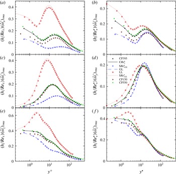
The root-mean-squares (r.m.s.s) of the semilocally scaled turbulent vorticity fluctuations
 $\hat{\unicode[STIX]{x1D74E}}^{\prime }=\unicode[STIX]{x1D6FB}\times \hat{\boldsymbol{u}}^{\prime }$
for streamwise (
 $\hat{\unicode[STIX]{x1D714}}_{x}^{\prime }$
), wall-normal (
 $\hat{\unicode[STIX]{x1D714}}_{y}^{\prime }$
) and spanwise (
 $\hat{\unicode[STIX]{x1D714}}_{z}^{\prime }$
) directions are shown in figure 10. Figure 10(a,c,e) shows the vorticity normalised by the wall-based viscous scale
 $h/Re_{\unicode[STIX]{x1D70F}}$
as a function of
 $y^{+}$
, whereas the vorticity normalised by the semilocal viscous scale
 $h/Re_{\unicode[STIX]{x1D70F}}^{\star }$
as a function of
 $y^{\star }$
is shown in figure 10(b,d,f). According to our previous work (Patel et al.
Reference Patel, Peeters, Boersma and Pecnik2015), quasisimilar vorticity statistics are obtained for cases with quasisimilar
 $Re_{\unicode[STIX]{x1D70F}}^{\star }$
profiles, even though the individual density and viscosity profiles differ. Comparison of cases with different
 $Re_{\unicode[STIX]{x1D70F}}^{\star }$
gradients in figure 10(a,c,e) shows considerable differences in terms of both magnitude and wall-normal location of peak values. On the other hand, the semilocal normalisation (figure 10
b,d,f) provides a reasonable collapse in regions away from the wall for comparable
 ${Re_{\unicode[STIX]{x1D70F}}^{\star }}_{c}$
, and it is also able to preserve the wall-normal locations of the peaks. However, in the near-wall region the semilocal scaling with
 $h/Re_{\unicode[STIX]{x1D70F}}^{\star }$
fails and does not provide a collapse of the vorticity profiles, even though the van Driest transformed mean spanwise vorticity scales well with
 $h/Re_{\unicode[STIX]{x1D70F}}^{\star }$
(see figure 5
d). In the following, we will make several comments on statistics of semilocally normalised vorticity fluctuations.
-
(i) It is known that even for constant-property cases the
$x$
and
$z$
vorticity fluctuation components increase with Reynolds number, whereas the
$y$
component shows
$Re_{\unicode[STIX]{x1D70F}}$
independence (Antonia & Kim Reference Antonia and Kim1994). This
$Re_{\unicode[STIX]{x1D70F}}$
dependence is particularly prominent for the the low-Reynolds-number case CP150 (brown triangles, colour online). -
(ii) For the variable-property cases, it is interesting to see that the cases with
$\text{d}Re_{\unicode[STIX]{x1D70F}}^{\star }/\text{d}y>0$
have the highest magnitude of the semilocally scaled
$\hat{\unicode[STIX]{x1D714}}_{x}^{\prime }$
in the near-wall region, although their
$Re_{\unicode[STIX]{x1D70F}}$
values are the lowest (
$Re_{\unicode[STIX]{x1D70F}}=150$
). The opposite occurs for cases with decreasing
$Re_{\unicode[STIX]{x1D70F}}^{\star }$
away from the wall. There, the streamwise vorticity fluctuations are the lowest, even for comparatively high values of
$Re_{\unicode[STIX]{x1D70F}}=395$
. This is clearly a variable-property effect that is in contrast to the Reynolds number dependence as discussed in point (i). Similar observations can be made for the
$y$
and
$z$
components. The semilocally scaled r.m.s. values of
$\hat{\unicode[STIX]{x1D714}}_{y}^{\prime }$
and
$\hat{\unicode[STIX]{x1D714}}_{z}^{\prime }$
are the highest in the near-wall region for cases with
$\text{d}Re_{\unicode[STIX]{x1D70F}}^{\star }/\text{d}y>0$
, and vice versa. -
(iii) For cases with
$\text{d}Re_{\unicode[STIX]{x1D70F}}^{\star }/\text{d}y>0$
, the
$z$
component has a maximum at approximately the same location where the van Driest transformed mean spanwise vorticity also shows a maximum. This is in agreement with the inflection point of the van Driest transformed mean velocity, which causes the flow to become more unstable, as mentioned in § 4.1. For cases with
$\text{d}Re_{\unicode[STIX]{x1D70F}}^{\star }/\text{d}y<0$
, the fluctuations fall off rapidly away from the wall.


The failure of the semilocal scaling is presumably caused by both structural changes in turbulence and strong non-local interactions between structures in the buffer layer and viscous sublayer which will be discussed in detail in § 5.
(a) Normal Reynolds stress anisotropies and (b) Reynolds shear stress anisotropy as a function of
 $y^{\star }$
.

4.3 Turbulent stress anisotropy
As described earlier, and as discussed in our previous work (Patel et al.
Reference Patel, Peeters, Boersma and Pecnik2015), gradients of
 $Re_{\unicode[STIX]{x1D70F}}^{\star }$
have a large effect on inter-component energy transfer and thus on turbulence anisotropy. The anisotropy tensor is defined as
 $$\begin{eqnarray}\unicode[STIX]{x1D623}_{ij}=\frac{\widetilde{\hat{u} _{i}^{\prime }\hat{u} _{j}^{\prime }}}{2k}-\unicode[STIX]{x1D6FF}_{ij}\frac{1}{3},\end{eqnarray}$$
with the turbulent kinetic energy
 $k=\widetilde{\hat{u} _{k}^{\prime }\hat{u} _{k}^{\prime }}/2$
and
 $\unicode[STIX]{x1D6FF}_{ij}$
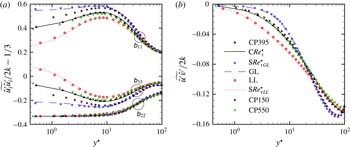
the Kronecker delta. Figure 11(a) shows that for cases with
 $\text{d}Re_{\unicode[STIX]{x1D70F}}^{\star }/\text{d}y<0$
, an increase in the streamwise component
 $\unicode[STIX]{x1D623}_{11}$
and a decrease in the spanwise component
 $\unicode[STIX]{x1D623}_{33}$
occurs in the near-wall region if compared with cases with
 $\text{d}Re_{\unicode[STIX]{x1D70F}}^{\star }/\text{d}y=0$
. The opposite is seen for cases with
 $\text{d}Re_{\unicode[STIX]{x1D70F}}^{\star }/\text{d}y>0$
. The wall-normal component
 $\unicode[STIX]{x1D623}_{22}$
, however, is not influenced by gradients in
 $Re_{\unicode[STIX]{x1D70F}}^{\star }$
. The increase in
 $\unicode[STIX]{x1D623}_{11}$
for cases with
 $\text{d}Re_{\unicode[STIX]{x1D70F}}^{\star }/\text{d}y<0$
indicates a decrease in the redistribution of turbulent energy from the streamwise direction to the other two directions. The component
 $\unicode[STIX]{x1D623}_{12}$
, which is the ratio of turbulent shear stress and turbulent kinetic energy, is shown in figure 11(b). It decreases for cases with
 $\text{d}Re_{\unicode[STIX]{x1D70F}}^{\star }/\text{d}y<0$
, indicating a reduced momentum transfer in spite of higher turbulent kinetic energy, while the reverse is true for cases with
 $\text{d}Re_{\unicode[STIX]{x1D70F}}^{\star }/\text{d}y>0$
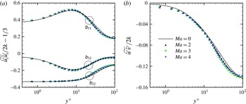
. The same quantities are also shown in figure 12 for the adiabatic supersonic turbulent boundary layer cases from Bernardini & Pirozzoli (Reference Bernardini and Pirozzoli2011) and Pirozzoli & Bernardini (Reference Pirozzoli and Bernardini2011), and compared with reference boundary layer data from Jiménez et al. (Reference Jiménez, Hoyas, Simens and Mizuno2010). No significant changes in anisotropy are noticeable since
 $\text{d}Re_{\unicode[STIX]{x1D70F}}^{\star }/\text{d}y\approx 0$
in the near-wall region. The change in anisotropy for cases with
 $\text{d}Re_{\unicode[STIX]{x1D70F}}^{\star }/\text{d}y\neq 0$
is linked to modifications in turbulent structures that will be discussed next.
(a) Normal Reynolds stress anisotropies and (b) Reynolds shear stress anisotropy as a function of
 $y^{+}$
for adiabatic supersonic boundary layers obtained from Bernardini & Pirozzoli (Reference Bernardini and Pirozzoli2011) and Pirozzoli & Bernardini (Reference Pirozzoli and Bernardini2011), and compared with reference boundary layer data from Jiménez et al. (Reference Jiménez, Hoyas, Simens and Mizuno2010).

5 Turbulent structures
Here, we investigate the influence of near-wall
 $Re_{\unicode[STIX]{x1D70F}}^{\star }$
gradients on the characteristics of near-wall streaks and quasistreamwise vortices, which are both known to be the dominant structures in near-wall turbulence, in order to provide a mechanistic description for the modulated statistics.
5.1 Near-wall streaks
For constant-property cases, the near-wall streak spacing in the viscous sublayer remains remarkably constant over a wide range of Reynolds numbers (Klewicki et al.
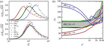
Reference Klewicki, Metzger, Kelner and Thurlow1995). Figure 13(a) shows the normalised premultiplied spanwise spectrum of the semilocally scaled streamwise velocity fluctuation
 $k_{z}E_{\hat{u} ^{\prime }\hat{u} ^{\prime }}/\overline{\hat{u} ^{\prime }\hat{u} ^{\prime }}$
at
 $y^{\star }\approx 0.5$
(top) and
 $y^{\star }\approx 13$
(bottom) as a function of the semilocally scaled wavelength
 $\unicode[STIX]{x1D706}_{z}^{\star }=\unicode[STIX]{x1D706}_{z}Re_{\unicode[STIX]{x1D70F}}^{\star }/h$
. The peak location of the spectrum represents the mean streak spacing, and it can be seen that at
 $y^{\star }\approx 13$
the spacing is the same for all cases (
 $\unicode[STIX]{x1D706}_{z}^{\star }\approx 120$
). This is one of the few similarities that variable-property and constant-property cases share. On the other hand, at
 $y^{\star }\approx 0.5$
only the constant-property cases (CP395, CP150, CP550) and the variable-property case
 $\text{C}Re_{\unicode[STIX]{x1D70F}}^{\star }$
show a similar streak spacing of
 $\unicode[STIX]{x1D706}_{z}^{\star }=\unicode[STIX]{x1D706}_{z}^{+}\approx 110$
, whereas the variable-property cases with
 $\text{d}Re_{\unicode[STIX]{x1D70F}}^{\star }/\text{d}y\neq 0$
show a modulation in streak spacing. The cases with
 $\text{d}Re_{\unicode[STIX]{x1D70F}}^{\star }/\text{d}y<0$
(blue lines and symbols, colour online) show an increased streak spacing of
 $\unicode[STIX]{x1D706}_{z}^{\star }\approx 220$
, while
 $\unicode[STIX]{x1D706}_{z}^{\star }\approx 50$
for cases with
 $\text{d}Re_{\unicode[STIX]{x1D70F}}^{\star }/\text{d}y>0$
(red lines and symbols, colour online). Figure 13(b) gives an overview of the near-wall streak spacing as a function of
 $y^{\star }$
. The lines in the plot indicate the boundaries where
 $k_{z}E_{\hat{u} ^{\prime }\hat{u} ^{\prime }}/\overline{\hat{u} ^{\prime }\hat{u} ^{\prime }}$
is 96 % of the peak value at a certain
 $y^{\star }$
location. It can be seen that the mean streak spacing appears to become universal after
 $y^{\star }\approx 12-13$
, while it deviates significantly in the viscous sublayer for cases with
 $\text{d}Re_{\unicode[STIX]{x1D70F}}^{\star }/\text{d}y\neq 0$
. This deviation is not surprising, because of the fact that the sublayer flow is known to be induced by advecting dominant structures in the buffer layer (Kim & Hussain Reference Kim and Hussain1993). The wall-normal location of the dominant structures is also found to be universal in semilocal units, as shown by Pei et al. (Reference Pei, Chen, Hussain and She2013), using a vorticity–velocity correlation in supersonic channel flows with isothermal walls at different Mach numbers. The strong non-local influence of turbulence structures in the buffer layer on the near-wall region creates a disparity between the semilocal scales and the actual turbulent scales in the sublayer.
(a) Normalised premultiplied spanwise spectrum
 $k_{z}E_{\hat{u} ^{\prime }\hat{u} ^{\prime }}/\overline{\hat{u} ^{\prime }\hat{u} ^{\prime }}$
as a function of
 $\unicode[STIX]{x1D706}_{z}^{\star }$
at
 $y^{\star }\approx 0.5$
(top) and
 $y^{\star }\approx 13$
(bottom). (b) Plot of
 $\unicode[STIX]{x1D706}_{z}^{\star }$
as a function of
 $y^{\star }$
obtained using bands of
 $k_{z}E_{\hat{u} ^{\prime }\hat{u} ^{\prime }}/\overline{\hat{u} ^{\prime }\hat{u} ^{\prime }}$
with values larger than 96 % of its maximum value; black, brown, green, blue and red lines correspond to cases CP395, CP150, CP550, GL and LL respectively; the grey region corresponds to the case
 $\text{C}Re_{\unicode[STIX]{x1D70F}}^{\star }$
.

5.2 Vortical structures
The three-dimensional swirling strength
 $\unicode[STIX]{x1D6EC}_{ci}(x,y,z)$
, which is based on the imaginary part of the complex eigenvalue of the velocity gradient tensor (Zhou et al.
Reference Zhou, Adrian, Balachandar and Kendall1999), is used to identify the near-wall vortical structures. The swirling strength separates swirling from shearing motion, and it can be evaluated using the gradient tensor of the instantaneous or the fluctuating velocity field. It has been analytically shown that it is not possible to decouple the mean shear from the instantaneous field (Chen et al.
Reference Chen, Adrian, Zhong and Wang2014). In our investigations, we evaluate the swirling strength using the instantaneous velocity gradient tensor, because the local shear depends on the instantaneous field. Similarly to Wu & Christensen (Reference Wu and Christensen2006), we normalise the local swirling strength with its corresponding wall-normal r.m.s.
 $\unicode[STIX]{x1D6EC}_{ci}^{rms}(y)$
value, such that
 $\acute{\unicode[STIX]{x1D6EC}}_{ci}(x,y,z)=\unicode[STIX]{x1D6EC}_{ci}(x,y,z)/\unicode[STIX]{x1D6EC}_{ci}^{rms}(y)$
.
(a) Isosurfaces of swirling strength seen from the top; red isosurfaces correspond to positive vorticity while blue denotes negative vorticity; the contours show the low-speed streaks. The rectangular box corresponds to panel (b). (b) Isometric view of structures with real eigenvectors at the vortex centre; the grey colour corresponds to projection of the structures at the wall; vectors corresponding to positive vorticity are shown as blue while red denotes negative vorticity.

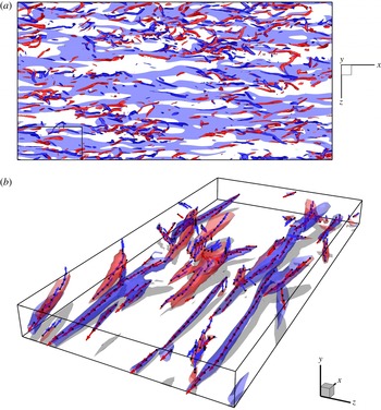
Figure 14(a) shows the top view of an isosurface of
 $\acute{\unicode[STIX]{x1D6EC}}_{ci}=1.5$
for case CP395 in the near-wall region up to
 $y^{+}\approx 50$
. As stated in previous studies (Robinson Reference Robinson1991; Jeong et al.
Reference Jeong, Hussain, Schoppa and Kim1997), the near-wall region is mostly populated by quasistreamwise vortices. The isosurfaces are coloured by the sign of their streamwise vorticity, where red denotes positive and blue negative vorticity (colour online). The figure also shows a slice of low-speed streaks at
 $y^{+}=13$
(seen as light blue online). A small section (black box) of the same instantaneous flow field is shown in an isometric view in figure 14(b), in order to show the inclination and elevation of these structures with respect to the wall (the grey shades are projections of the isosurfaces onto the wall). As noted by Jeong et al. (Reference Jeong, Hussain, Schoppa and Kim1997), the structures with positive vorticity tend to tilt in the negative direction and those with negative vorticity tend to tilt in the positive direction with respect to the streamwise direction within the
 $x$
–
 $z$
plane. This tilting is correlated with the waviness of streaks and it is associated with transfer of streamwise turbulent energy to spanwise and wall-normal components (Jeong et al.
Reference Jeong, Hussain, Schoppa and Kim1997). Therefore, study of the orientation of these structures can clarify the changes in anisotropy that occur in flows with gradients in
 $Re_{\unicode[STIX]{x1D70F}}^{\star }$
.
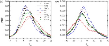
Probability density function of projection angle of eigenvector
 $\unicode[STIX]{x1D708}_{r}$
at
 $y^{\star }=13$
: (a) inclination angle
 $\unicode[STIX]{x1D703}_{xy}$
; (b) tilting angle
 $\unicode[STIX]{x1D703}_{xz}$
.

The orientation of the vortical structures can be characterised by the real eigenvector
 $\unicode[STIX]{x1D708}_{r}$
of the velocity gradient tensor, which is able to differentiate the swirling direction from the vorticity direction (Pirozzoli et al.
Reference Pirozzoli, Bernardini and Grasso2008; Gao, Ortiz-Duenas & Longmire Reference Gao, Ortiz-Duenas and Longmire2011). However, before evaluating the vortex orientation we must first find the vortex centre. This is done by performing the following steps. First, all of the grid points that correspond to the local maxima of the swirling strength
 $\unicode[STIX]{x1D6EC}_{ci}$
are flagged in all
 $y{-}z$
planes of the numerical domain. Next, the real eigenvector
 $\unicode[STIX]{x1D708}_{r}$
of these points is used to check whether the projection angles in the perpendicular planes, which define the lift and the tilt and are denoted as
 $\unicode[STIX]{x1D703}_{xy}$
and
 $\unicode[STIX]{x1D703}_{xz}$
, are within
 $\pm 45^{\circ }$
. If this condition is met, the points are retained, otherwise they are discarded. These steps are repeated to also find the vortex centres in the
 $z{-}x$
and
 $x{-}y$
planes of the computational domain. Finally, only the points with
 $\acute{\unicode[STIX]{x1D6EC}}_{ci}\geqslant 1.5$
are kept and used as the vortex centres. It should be noted that most of vortex centres were found in the
 $y{-}z$
plane, showing the dominance of quasistreamwise vortices. An outcome of this eduction procedure is given in figure 14(b), where the vortex centres with their corresponding eigenvectors are shown. Since eigenvectors can have either of the two opposing directions, the positive direction is chosen such that the dot product with the vorticity vector is positive. As is evident, the eigenvectors
 $\unicode[STIX]{x1D708}_{r}$
provide an excellent measure of the orientation axis of the vortical structures. We will now apply this procedure to obtain statistics of the inclination and tilting angles to draw conclusions on turbulence modulation for all constant- and variable-property cases investigated in this work.
The probability density functions (p.d.f.s) of the inclination angle
 $\unicode[STIX]{x1D703}_{xy}$
and tilting angle
 $\unicode[STIX]{x1D703}_{xz}$
of the vortical structures at
 $y^{\star }=13$
are shown in figure 15. Similarly to turbulence statistics, the orientation of vortical structures for cases with quasisimilar
 $Re_{\unicode[STIX]{x1D70F}}^{\star }$
profiles also shows quasisimilarity and is therefore independent of individual density and viscosity profiles. As shown in figure 15(a), an increase in
 $Re_{\unicode[STIX]{x1D70F}}$
from 150 to 550 for the constant-property cases increases the mode of the p.d.f. from
 $7^{\circ }$
to
 $8^{\circ }$
and broadens it, showing an increase in standard deviation. The variable-property cases with
 $\text{d}Re_{\unicode[STIX]{x1D70F}}^{\star }/\text{d}y<0$
(blue line and symbols, colour online) show a decrease in the mode of the p.d.f. (
 $6^{\circ }$
) and a decrease in standard deviation. The opposite is seen for cases with
 $\text{d}Re_{\unicode[STIX]{x1D70F}}^{\star }/\text{d}y>0$
(red line and symbols, colour online), which show an increase in the mode (
 $10^{\circ }$
) and a broadening of the distribution. These results show that lifting of coherent vortical structures reduces for cases with
 $\text{d}Re_{\unicode[STIX]{x1D70F}}^{\star }/\text{d}y<0$
, and increases for
 $\text{d}Re_{\unicode[STIX]{x1D70F}}^{\star }/\text{d}y>0$
. This is in agreement with our previous findings (Patel et al.
Reference Patel, Peeters, Boersma and Pecnik2015), where we observed that the streaks are stabilised and do not lift as intensely for cases with
 $\text{d}Re_{\unicode[STIX]{x1D70F}}^{\star }/\text{d}y<0$
, while they lift more intensely for cases with
 $\text{d}Re_{\unicode[STIX]{x1D70F}}^{\star }/\text{d}y>0$
.
The tilting of the structures is indicated in figure 15(b). Because the direction of the tilting is coupled to the sign of the streamwise vorticity, and the events related to positive and negative streamwise vorticity are symmetric, we only show tilting angles for positive streamwise vorticity. Only small changes can be seen for the constant-property cases, with the mode at approximately
 $\pm 8^{\circ }$
. For cases with
 $\text{d}Re_{\unicode[STIX]{x1D70F}}^{\star }/\text{d}y<0$
, the mode of the p.d.f.s occurs at
 $\pm 5^{\circ }$
and the distributions narrow. The reverse happens for cases with
 $\text{d}Re_{\unicode[STIX]{x1D70F}}^{\star }/\text{d}y>0$
, with the mode at
 $\pm 11^{\circ }$
and broader distributions.
We will now summarise the effects related to flows with variable properties and provide a mechanistic description to explain the observed turbulence modulations. In order to avoid switching between different cases, we will only use cases with
 $\text{d}Re_{\unicode[STIX]{x1D70F}}^{\star }/\text{d}y>0$
(the effects for cases with
 $\text{d}Re_{\unicode[STIX]{x1D70F}}^{\star }/\text{d}y<0$
are exactly opposite). The increase in magnitude of the van Driest transformed mean spanwise vorticity
 $-\text{d}\overline{u}^{vD}/\text{d}y$
increases the mean forcing in the spanwise direction, causing the increased tilting of vortical structures. The increased tilting results in stronger streak waviness, which then leads to increased turbulence activity, enabling the evolution of near-wall structures and the generation of stronger shear layers (Johansson, Alfredsson & Kim Reference Johansson, Alfredsson and Kim1991). The increased lifting of both streaks and vortical structures is therefore closely associated with an increase in tilting of the structures. This also explains the increase in shear stress anisotropy, which increases the momentum transfer in spite of lower turbulent kinetic energy. Furthermore, the increase in tilting angle also provides a structural interpretation for the increase in the pressure–strain correlation, which acts as a sink in the budget of the streamwise energy equation and therefore redistributes the streamwise turbulent energy in the other two directions. From Jeong et al. (Reference Jeong, Hussain, Schoppa and Kim1997), it is known that the preferential alignment of structures with respect to streamwise vorticity produces positive values of
 $\unicode[STIX]{x2202}u^{\prime }/\unicode[STIX]{x2202}x$
within the structure, and since
 $p^{\prime }$
is negative within the structure,
 $p^{\prime }\unicode[STIX]{x2202}u^{\prime }/\unicode[STIX]{x2202}x$
is also negative. Additionally, the spanwise asymmetry results in internal shear layers, where high-speed fluid collides with low-speed fluid, causing a positive
 $p^{\prime }$
and a negative
 $\unicode[STIX]{x2202}u^{\prime }/\unicode[STIX]{x2202}x$
, and hence
 $p^{\prime }\unicode[STIX]{x2202}u^{\prime }/\unicode[STIX]{x2202}x<0$
. The modulation in tilting of the structures therefore provides a physical interpretation of the modulated turbulence statistics.
6 Conclusion
The effects of strong near-wall gradients in density and viscosity on the mean velocity scaling, near-wall turbulence statistics and turbulent structures are studied by performing DNS of a fully developed channel flow under the low-Mach-number approximation of the Navier–Stokes equations. Five variable-property cases (
 $\text{C}Re_{\unicode[STIX]{x1D70F}}^{\star }$
,
 $\text{S}Re_{\unicode[STIX]{x1D70F}GL}^{\star }$
, GL, LL,
 $\text{S}Re_{\unicode[STIX]{x1D70F}LL}^{\star }$
) with different relations for density and viscosity as a function of temperature are investigated. The different density and viscosity profiles are parametrised by means of the semilocal Reynolds number
 $Re_{\unicode[STIX]{x1D70F}}^{\star }\equiv Re_{\unicode[STIX]{x1D70F}}\sqrt{(\overline{\unicode[STIX]{x1D70C}}/\overline{\unicode[STIX]{x1D70C}}_{w})}/(\overline{\unicode[STIX]{x1D707}}/\overline{\unicode[STIX]{x1D707}}_{w})$
, which is known from Patel et al. (Reference Patel, Peeters, Boersma and Pecnik2015) to be the governing parameter for turbulence statistics. The case
 $\text{C}Re_{\unicode[STIX]{x1D70F}}^{\star }$
corresponds to a constant wall-normal
 $Re_{\unicode[STIX]{x1D70F}}^{\star }$
profile; for cases
 $\text{S}Re_{\unicode[STIX]{x1D70F}GL}^{\star }$
and GL, the
 $Re_{\unicode[STIX]{x1D70F}}^{\star }$
profile decreases towards the channel centre (
 $\text{d}Re_{\unicode[STIX]{x1D70F}}^{\star }/\text{d}y<0$
), and for cases LL and
 $\text{S}Re_{\unicode[STIX]{x1D70F}LL}^{\star }$
,
 $Re_{\unicode[STIX]{x1D70F}}^{\star }$
increases towards the channel centre (
 $\text{d}Re_{\unicode[STIX]{x1D70F}}^{\star }/\text{d}y>0$
). Three constant-property cases (CP395, CP150, CP550) at different
 $Re_{\unicode[STIX]{x1D70F}}$
values are also investigated to distinguish any Reynolds number effects from effects caused by property gradients.
Strong near-wall gradients in
 $Re_{\unicode[STIX]{x1D70F}}^{\star }$
result in a failure to collapse the van Driest transformed mean velocity
 $\overline{u}^{vD}$
as a function of
 $y^{+}$
. An extension of the van Driest transformation that accounts for the gradients in
 $Re_{\unicode[STIX]{x1D70F}}^{\star }$
(
 $\text{d}\overline{u}^{\star }=(1+(y/Re_{\unicode[STIX]{x1D70F}}^{\star })\text{d}Re_{\unicode[STIX]{x1D70F}}^{\star }/\text{d}y)\,\text{d}\overline{u}^{vD}$
) is derived based on the compelling collapse of the viscous stresses
 $(h/Re_{\unicode[STIX]{x1D70F}}^{\star })\,\text{d}\overline{u}^{vD}/\text{d}y$
for all cases when plotted as a function of the semilocal wall coordinate
 $y^{\star }$
. A successful collapse of
 $\overline{u}^{\star }$
when plotted as a function of
 $y^{\star }$
was obtained for all of the investigated cases. The applicability of the transformation was also tested on adiabatic supersonic boundary layers of Bernardini & Pirozzoli (Reference Bernardini and Pirozzoli2011) and Pirozzoli & Bernardini (Reference Pirozzoli and Bernardini2011), which are known to show an excellent agreement of
 $\overline{u}^{vD}$
as a function of
 $y^{+}$
. The new transformed velocity collapses supersonic cases at different Mach numbers. However, the supersonic cases showed a small increase in the log-law additive constant when compared with an incompressible turbulent boundary layer. In a recent work, Trettel & Larsson (Reference Trettel and Larsson2016) derived a similar transformation in terms of density and viscosity gradients, and applied it successfully to supersonic channel flows with isothermal cooled walls.
Near-wall gradients in
 $Re_{\unicode[STIX]{x1D70F}}^{\star }$
also result in turbulence modification when compared with constant-property cases with similar
 $Re_{\unicode[STIX]{x1D70F}}$
values. Partial success in accounting for this change in turbulence is obtained using the semilocal scaling, which accommodates the changes in viscous scales using local fluid properties. The success of the semilocal scaling is evident for the profiles of Reynolds shear stress and viscous shear stress. However, statistics like the r.m.s. of vorticity fluctuations, which are sensitive to the strong non-local interactions of the buffer layer vortical structures with the viscous sublayer, show a poor collapse in the near-wall region using the semilocal scaling. These strong non-local interactions are evident from the semilocally scaled streak spacing which tends to become universal after
 $y^{\star }\approx 12{-}13$
, while it deviates significantly in the viscous sublayer for cases with
 $\text{d}Re_{\unicode[STIX]{x1D70F}}^{\star }/\text{d}y\neq 0$
. Furthermore, the failure of the semilocal scaling also occurs due to structural changes in turbulence that affect lifting and tilting of quasistreamwise vortices. These changes influence the Reynolds stress generation mechanism and the inter-component energy transfer for turbulent stresses. The influence of this failure on the scaling of the
 $\overline{u}^{\star }$
profile is negligible, since similarly to the Reynolds shear stress the mixing length is modified in the viscosity dominated region and therefore has a negligible influence on the transformed velocity profile.
The influence of
 $Re_{\unicode[STIX]{x1D70F}}^{\star }$
gradients on vortical structures was studied using the three-dimensional swirling strength based on the instantaneous velocity gradient tensor. The orientation of these structures was determined using the real eigenvector of the tensor at the vortex centre. The analysis shows that, similarly to constant-property cases, the near-wall region in variable-property flows is also mostly populated by quasistreamwise vortices that are slightly inclined away from the wall and tilted towards the spanwise direction. Similarly to turbulence statistics, the near-wall turbulent structures are also strongly governed by the
 $Re_{\unicode[STIX]{x1D70F}}^{\star }$
profile, and their dependence on individual density and viscosity profiles is negligible. Cases with
 $\text{d}Re_{\unicode[STIX]{x1D70F}}^{\star }/\text{d}y>0$
show an inflection point in
 $\overline{u}^{vD}$
, causing a higher strain with respect to the wall. This increase in strain increases the mean forcing in the spanwise direction, which results in an increase in tilting of quasistreamwise vortices. The increased tilting of the structures increases the asymmetry of the streaks, which are known to play an important role in maintaining the near-wall cycle and generation of strong shear layers (Johansson et al.
Reference Johansson, Alfredsson and Kim1991). This increased turbulence activity also causes an increased lifting of the structures and explains why cases with
 $\text{d}Re_{\unicode[STIX]{x1D70F}}^{\star }/\text{d}y>0$
show an increased momentum transfer in spite of lower turbulent kinetic energy. The increase in tilting of the structures also provides a physical interpretation for the increase in negative pressure–strain, which enables transfer of streamwise fluctuation energy towards spanwise and wall-normal components (Jeong et al.
Reference Jeong, Hussain, Schoppa and Kim1997). The opposite is true for cases with
 $\text{d}Re_{\unicode[STIX]{x1D70F}}^{\star }/\text{d}y<0$
.
Acknowledgements
The authors would like to acknowledge access to large-scale computing facilities from the Netherlands Organisation for Scientific Research (NWO) through a grant with the dossier number SSH-223-13. The authors also wish to thank Dr S. Pirozzoli for providing additional information for his DNS data of supersonic turbulent boundary layers.