1 Introduction
Coherent structures within the earth’s oceans cascade in scale from planetary to meso and sub-meso, then down to scales smaller than sea spray, whereas global simulations of the oceans are forced to cut off in the sub-meso range. At the smaller scale end of the sub-meso range are structures long known to mariners by their surface footprints, seen as long, frothy, almost parallel, wind-aligned lines or windrows. The footprints are those of Langmuir circulation (LC) that are comprised of multiple counter-rotating vortex pairs (Langmuir Reference Langmuir1938) near the ocean surface that form in the presence of surface waves and wind, and grow in cross-section to the size of sports stadiums (Plueddemann et al. Reference Plueddemann, Smith, Farmer, Weller, Crawford, Pinkel, Vagle and Gnanadesikan1996). When present, LC help not only to mix the upper ocean (Langmuir Reference Langmuir1938; Smith Reference Smith1992) but convey nutrients into it (Thorpe Reference Thorpe2004) and provide transport to phytoplankton as they ride from the ocean depths to the surface and then back down again (Barstow Reference Barstow1983). Furthermore, since each few metres of the surface mixed layer has the same heat content as the whole atmosphere above it (Gill Reference Gill1982) and since LC mix that heat downwards, the depth to which LC penetrate is important, because it affects the local heat content and thus thermodynamics.
Although peta-scale computers are able to simulate the whole sub-meso scale range in regional calculations, albeit crudely (Li et al. Reference Li, Webb, Fox-Kemper, Craig, Danabasoglu, Large and Vertenstein2016; Pearson et al. Reference Pearson, Fox-Kemper, Bachman and Bryan2017), computation of the smaller scale end of it where LC live, remains at the limit of global calculations. Nevertheless, representation of LC in the later, even in a simple parametric form, were found by Babanin, Ganopolski & Phillips (Reference Babanin, Ganopolski and Phillips2009) to provide a richness to the computations not before seen and as computing power has increased, attention has turned to incorporating more extensive parametric representations of them. That aspiration has in turn spawned renewed interest in the aetiology of LC and our purpose here is to focus on hitherto unexplored aspects of their nonlinear dynamics, vis à vis LC resonating with LC.
To proceed we turn to the prevailing theory for the evolution of LC, viz. the mean field Craik–Leibovich (CL) equations of Craik & Leibovich (Reference Craik and Leibovich1976) and since the penetration depth is set by LC spacing and aspect ratio, question how each is affected by nonlinearity. Of course both measures have been thoroughly explored using the linearised form of the CL equations in various settings, such as in deep water (see e.g. Leibovich Reference Leibovich1983; Thorpe Reference Thorpe2004), in layers separated by a thermocline on deep water (e.g. Cox & Leibovich Reference Cox and Leibovich1993; Leibovich & Tandon Reference Leibovich and Tandon1993), and in shallow water (Phillips & Dai Reference Phillips and Dai2014; Hayes & Phillips Reference Hayes and Phillips2016, Reference Hayes and Phillips2017). Also while there are instances where linear instability theory (Phillips Reference Phillips2001, Reference Phillips2002) captures observed (Smith Reference Smith1992) LC spacings in deep water reasonably well, there are also instances where linear theory is noticeably in error, particularly in shallow waters (Marmorino, Smith & Lindemann Reference Marmorino, Smith and Lindemann2005). Less attention has been paid to the role nonlinearities play in LC spacing, although some aspects of the shallow water case are captured by nonlinear asymptotic theory (Hayes & Phillips Reference Hayes and Phillips2017). There is also a body of work on oscillatory instabilities in strongly supercritical nonlinear conditions (e.g. Moroz & Leibovich Reference Moroz and Leibovich1985) and studies of pattern formation using both weakly and strongly nonlinear LC theories (e.g. Bhaskaran & Leibovich Reference Bhaskaran and Leibovich2002; Zhang et al. Reference Zhang, Chini, Julien and Knobloch2015).
To be clear, the spacings of interest here are those for a pair (two rolls) of the largest LC, or more precisely most dominant LC, in a discrete spectrum of LC that together comprise Langmuir turbulence (McWilliams, Sullivan & Moeng Reference McWilliams, Sullivan and Moeng1997). That said, LC spacing is subject to change abruptly, as evidenced by the sporadic presence of Y-junctions, which are a hallmark feature in surface patterns of observed (Farmer & Li Reference Farmer and Li1995) and numerical Langmuir turbulence (McWilliams et al. Reference McWilliams, Sullivan and Moeng1997; Tsai et al. Reference Tsai, Chen, Lu and Garbe2013; Tsai, Chen & Lu Reference Tsai, Chen and Lu2015). Y-junctions are viewed either as the merger of two distinct windrows (via the arms of the Y) or the splitting of a single windrow (the stalk of the Y) into two (arms). Of course these views are identical in the absence of a reference direction, but when the frame is determined by wind direction, the preferred formation is a merger, with the stalk of the Y pointed downwind (Farmer & Li Reference Farmer and Li1995; Bhaskaran & Leibovich Reference Bhaskaran and Leibovich2002). Be that as it may, of key interest is the abrupt change in LC spacing and what bifurcations trigger it.
Of course jumps in spacing can result from changes in Prandtl number, as linear instability studies of LC show (Phillips Reference Phillips2001), but their more common occurrence is likely the result of a nonlinear cascade, through the excitation and amplification of harmonic and subharmonic modes. Energy is then transferred from the fundamental into the modes, which may remain in isolation of each other or interact; transfer being optimal when the interacting modes resonate. Indeed, downwind-modulated 1 : 2 spatial resonance is observed by Zhang et al. (Reference Zhang, Chini, Julien and Knobloch2015) in their fully nonlinear numerical study of dynamic surface patterns arising from LC.
Curiously, although Chini & Leibovich (Reference Chini and Leibovich2003, Reference Chini and Leibovich2005) theoretically explore resonance in the context of LC resonating with internal waves, the only theoretical work on LC resonating with LC would appear to be a Woods Hole Oceanographic Institution report by Maultsby (Reference Maultsby, Knobloch and Weiss2012). Moreover, although various aspects of LC undergoing nonlinear mode-amplification in isolation have been undertaken (see e.g. Cox et al. Reference Cox, Leibovich, Moroz and Tandon1992a ,Reference Cox, Leibovich, Moroz and Tandon b ), there would appear to have been no analytical work on the Eckhaus instability of such LC. Our purpose here, therefore, is to analyse the nonlinear amplification of such modes, be they in isolation or in resonance, with the object of investigating the bifurcation or bifurcations underlying spacing change.
Of course the story is vastly different in the area of convection, where 1 : 2 and 1 : 3 resonance mode interactions based upon amplitude equations for modes with spanwise wavenumbers
 $l$
and
 $2l$
, or
 $l$
and
 $3l$
, have been widely studied (see e.g. Proctor & Jones Reference Proctor and Jones1988; Mizushima & Fujimura Reference Mizushima and Fujimura1992; Mizushima Reference Mizushima1993; Cox Reference Cox1996). Therein, two scenarios are considered: in the first, which Maultsby (Reference Maultsby, Knobloch and Weiss2012) employed to consider 1 : 2 resonance in LC, the modes are positioned on the neutral curve, which means that integer ratios are possible only at specific Rayleigh numbers (or other parameter). In the second, the fundamental is set as the least stable linear mode, so that any Rayleigh number above critical may be utilised, provided the harmonic is likewise linearly unstable.
Both scenarios are studied in convection problems because both are physically realisable there (Fujimura & Nagata Reference Fujimura and Nagata1998). But in the context of LC, and in the absence of very specific external oscillatory forcing to excite modes on the neutral curve, the veracity of the first is less compelling. Because of that we will not explore the first scenario and instead concentrate on the second, which has not previously been applied to LC and rests upon modes known to be linearly unstable.
To that end we consider LC in their simplest sense, viz. wind aligned and spanwise periodic as seen in the photographs of Szeri (Reference Szeri1996), and describe their evolution using the CL equations, which in the absence of stratification can be written to contain only one parameter, the Rayleigh number
 ${\mathcal{R}}$
. Instability to LC can then occur when the current driven by wind, in combination with Lagrangian drift arising from the waves, is depth dependent and of the same sense, the simplest case being when depth dependence is linear. We then arrive at a construct for LC in layers employed in the asymptotic studies of Cox & Leibovich (Reference Cox and Leibovich1993) and others (Hayes & Phillips Reference Hayes and Phillips2016, Reference Hayes and Phillips2017), whose interest lay with the free surface boundary conditions and whose findings are relevant here.
Specifically, Cox & Leibovich (Reference Cox and Leibovich1993) questioned why Neumann or stress-free conditions on the perturbation motion ensure the wavenumber
 $l$
is non-zero at the onset to instability in studies of LC in deep water (Craik Reference Craik1977), yet require
 $l=0$
in layers. Their resolution was that Neumann conditions fail to reflect coupling between the perturbed motion and the extra stress it must produce, implying that mixed or Robin boundary conditions be employed to capture it, a result later formalised by Phillips & Dai (Reference Phillips and Dai2014). Moreover, with mixed conditions at the free surface and Neumann at the bottom, the extra stress has a further role, that of symmetry breaking. So, if we specify the level of the extra stress by the Biot number
 $\unicode[STIX]{x1D6FE}$
, then our construct for the evolution of LC in layers has two parameters
 $\unicode[STIX]{x1D6FE}$
and
 ${\mathcal{R}}$
, and our task is to determine the role each plays on the nonlinear dynamics of LC.
After formally posing the problem in § 2, we go on in § 3 to explore the linear case and determine how
 $\unicode[STIX]{x1D6FE}$
affects instability and the onset to it. Of note as
 $\unicode[STIX]{x1D6FE}$
increases from zero to unity, is that the neutral curves evolve from asymmetric near onset to almost parabolic, a feature that must likewise be reflected by the Ginzburg–Landau equation used in § 4 to explore the nonlinear dynamics of single modes. That necessitates taking the Ginzburg–Landau equation to quartic rather than cubic order, as is typical when the bifurcation is supercritical, as it is here. We then proceed with an Eckhaus instability analysis and find that solitary harmonic modes are seldom excited. In view of these limitations, we then in §§ 5–6 derive coupled amplitude equations of Stuart-Landau type to explore 1 : 2 and 1 : 3 resonant mode interactions. After first exploring the nonlinear dynamics at fixed
 $\unicode[STIX]{x1D6FE}$
, we go on in § 7 to vary both
 $\unicode[STIX]{x1D6FE}$
and
 ${\mathcal{R}}$
. Our findings are discussed in § 8.
2 Governing equations
2.1 Background
We consider longitudinal vortex modes, to wit LC, that form through an instability arising from the interaction of neutral surface gravity waves with a sheared current beneath them. In crafting the problem we set
 $z$
vertical (positive upwards) and
 $y$
cross-stream and align the direction of travel of the waves with that of the shear, namely in
 $x$
. Accordingly we denote the current or mean flow by
 $U(z)$
with component velocities by
 $\boldsymbol{u}=(u,v,w)$
in
 $(x,y,z)$
. That said, it is important to realise that three time scales are at play, namely the period of the waves (typically seconds), that of the mean flow about which the LC evolve (tens of minutes) and that of the LC themselves (tens of minutes). With that mindset, Craik & Leibovich (Reference Craik and Leibovich1976) employed the methods of multiple scales to derive a set of mean field equations, the CL equations, that describe the evolution of LC in an irrotational wave field expressed by its Lagrangian drift
 $D=D(y,z)$
, which results from the rectification of nonlinear wave–wave interactions. They went on to show that LC are excited by the interaction of shear with the drift. In fact they exposed two candidate instabilities to LC: CL1, an algebraically growing instability when
 $D$
is dependent of
 $y$
(Craik & Leibovich Reference Craik and Leibovich1976) and an exponentially growing instability CL2, when
 $D$
is independent of
 $y$
(Craik Reference Craik1977). Of the two instabilities, however, CL2 has attracted the most attention because in a random spectrum of waves, drift dependence in
 $y$
is phase averaged out. That said, and in contrast to CL1 which is easily reproduced in the laboratory (Faller Reference Faller1978; Faller & Caponi Reference Faller and Caponi1978), CL2 is not reproducible there because of scaling considerations (Melville, Shear & Veron Reference Melville, Shear and Veron1998), although it has been realised in direct numerical computations (Tsai et al.
Reference Tsai, Lu, Chen, Dai and Phillips2017). Of course stratification can also play a role and is captured by an energy equation (Leibovich Reference Leibovich1977) that complements the CL equations.
Others (Leibovich Reference Leibovich1980; Craik Reference Craik1985; Holm Reference Holm1996; Phillips Reference Phillips1998a
) have since derived the CL equations directly from Andrews & McIntyre’s (Reference Andrews and McIntyre1978) generalised Lagrangian mean equations but the most succinct, perhaps canonical, derivation follows directly from Kelvin’s circulation theorem (Leibovich Reference Leibovich1997). All, of course, invoke a Lagrangian average, but because the average is taken only over scales characteristic of the wave field, the mean field remains dependent on
 $x$
and
 $t$
, albeit over longer time and spatial scales, in accord with photographs of the surface footprints of LC. However, in contrast to Görtler vortices, where streamwise (
 $x$
) variations strongly influence instability (Hall Reference Hall1983), non-parallel effects influence the linearly most unstable growth of LC only weakly (Leibovich & Tandon Reference Leibovich and Tandon1993). Because of that
 $x$
-variations are largely excluded in instability studies of LC, thereby allowing their evolution to be viewed from the
 $(y,z)$
plane. The perturbation velocity field is then comprised of a component
 $u$
about
 $U$
aligned in
 $x$
together with cross-stream
 $(y,z)$
motions
 $(v,w)$
. In the terminology of the vortex-wave-interaction community (Deguchi & Hall Reference Deguchi and Hall2014), the
 $u$
-components are denoted streaks and the
 $(v,w)$
components rolls; streaks and rolls together constitute LC, although the mechanisms sustaining rolls and streaks in LC and in wall bounded shear flows would seem to be distinct (Phillips Reference Phillips2015).
Herein we too confine attention to the CL2 instability and exclude variations in
 $x$
; we also exclude stratification. The ensuing form of the CL equations may be rescaled in various ways, but we largely follow Phillips & Dai (Reference Phillips and Dai2014), in which variables are scaled in terms of the layer depth
 $\mathfrak{h}$
, a characteristic Eulerian velocity
 $\mathscr{U}$
, a characteristic Lagrangian velocity
 $\mathscr{D}$
and the turbulent eddy viscosity
 $\unicode[STIX]{x1D708}_{T}$
. Length then scales as
 $(x,y,z)\mathfrak{h}$
, time as
 $t\mathfrak{h}^{2}\unicode[STIX]{x1D708}_{T}^{-1}$
and Eulerian velocities as
 $$\begin{eqnarray}\displaystyle [(U(z,\unicode[STIX]{x1D70F})+u(y,z,t))\mathscr{U},(v(y,z,t),w(y,z,t))\unicode[STIX]{x1D708}_{T}/h], & & \displaystyle\end{eqnarray}$$
with the Lagrangian drift velocity
 $\mathscr{D}D$
.
The CL equations subsequently pare into equations for the mean
 $U$
and secondary flow
 $(u,v,w)$
that evolve on disparate times scales
 $\unicode[STIX]{x1D70F}$
and
 $t$
(see Phillips & Dai (Reference Phillips and Dai2014)), viz.
 $$\begin{eqnarray}\displaystyle U_{\unicode[STIX]{x1D70F}}-U_{zz}=-G\quad \text{and}\quad u_{t}-\unicode[STIX]{x1D6FB}^{2}u=U^{\prime }\unicode[STIX]{x1D713}_{y}+J(\unicode[STIX]{x1D713},u), & & \displaystyle\end{eqnarray}$$
while the rolls are captured by the stream function
 $\unicode[STIX]{x1D713}(y,z,t)$
through
 $$\begin{eqnarray}\displaystyle (\unicode[STIX]{x2202}_{t}-\unicode[STIX]{x1D6FB}^{2})\unicode[STIX]{x1D6FB}^{2}\unicode[STIX]{x1D713}={\mathcal{R}}D^{\prime }u_{y}+J(\unicode[STIX]{x1D713},\unicode[STIX]{x1D6FB}^{2}\unicode[STIX]{x1D713}) & & \displaystyle\end{eqnarray}$$
in which
 $(v,w)=(\unicode[STIX]{x1D713}_{z},-\unicode[STIX]{x1D713}_{y})$
, the Jacobian
 $J(a,b)=a_{y}b_{z}-a_{z}b_{y}$
and
 $U$
may be driven by a mean streamwise body force
 $G$
(Phillips, Dai & Tjan Reference Phillips, Dai and Tjan2010). Finally, since (2.2) presumes the CL2 instability in which drift is independent of
 $y$
then, on using a prime to denote
 $\text{d}/\text{d}z$
, differential drift is
 $D^{\prime }(z)$
and the mean shear is
 $U^{\prime }(z)$
.
The flow is unstable to CL2 whenever
 $D^{\prime }U^{\prime }>0$
(Leibovich Reference Leibovich1983) over at least a part of the domain (Phillips & Dai Reference Phillips and Dai2014), subject to a lower bound in the Rayleigh number
 ${\mathcal{R}}$
, where
 $$\begin{eqnarray}\displaystyle {\mathcal{R}}=\frac{\mathscr{U}\mathscr{D}\mathfrak{h}^{2}}{\unicode[STIX]{x1D708}_{T}^{2}}. & & \displaystyle\end{eqnarray}$$
That said, it remains to specify the scales
 $\mathscr{D}$
and
 $\mathscr{U}$
, for which there are various choices. Phillips & Dai (Reference Phillips and Dai2014), for example, define them as values of drift and mean velocity at the free surface, whereas we employ our two other scales and define
 $\mathscr{U}$
in terms of the friction velocity
 $u_{\ast }$
at the free surface, to yield
 $\mathscr{U}=u_{\ast }^{2}\mathfrak{h}/\unicode[STIX]{x1D708}_{T}$
.
2.2 Boundary conditions
Studies of LC fall into two categories: those in non-stratified deep water (deep in the sense of deep water waves) and those in layers, which may be shallow in the sense of shallow water waves or atop deeper water separated by a thermocline. Our interest is with LC in layers that, in view of our scaling, span
 $z\in [-1,0]$
and thus require boundary conditions at the mean free surface
 $z=0$
and beneath it at
 $z=-1$
. Our expectation, of course, is that since Neumann conditions imposed on the linearised form of (2.2) ensure onset at non-zero spanwise wavenumber in deep water (Craik Reference Craik1977), the same should hold for a layer, but that is not so; on the contrary, Neumann conditions ensure onset occurs at zero spanwise wavenumber. This peculiarity first emerged in numerical studies of LC (Leibovich & Paolucci Reference Leibovich and Paolucci1980) which always grew to fill the computational box; it remained a conundrum until Cox & Leibovich (Reference Cox and Leibovich1993) questioned the veracity of Neumann boundary conditions.
In particular they noted that Neumann conditions ignore the coupling that occurs between the perturbed motion and the extra stress it produces at the free surface and argued that the Neumann term should be supplemented by the extra stress, to realise mixed or Robin boundary conditions. Specifically, Cox & Leibovich (Reference Cox and Leibovich1993) postulate boundary conditions of the generic form
 $u^{\prime }+\unicode[STIX]{x1D6FE}u=\unicode[STIX]{x1D713}^{\prime \prime }+\unicode[STIX]{x1D6FE}\unicode[STIX]{x1D713}^{\prime }=0$
, in which the Biot number
 $\unicode[STIX]{x1D6FE}$
represents the magnitude of the extra stress, noting that
 $\unicode[STIX]{x1D6FE}$
may be different at the top and bottom of the layer and that Neumann conditions are recovered when
 $\unicode[STIX]{x1D6FE}=0$
. They went on to show that mixed conditions indeed ensure the spanwise wavenumber is non-zero at onset. Phillips & Dai (Reference Phillips and Dai2014) later derived the free surface boundary conditions formally and show that the extra stress terms are indeed present, albeit premultiplied by
 $\unicode[STIX]{x1D6FE}$
s that are functions of the spanwise and streamwise wavenumbers and allow
 $\unicode[STIX]{x1D6FE}\in (0,1]$
.
Of key interest then was the role played by the extra stress in the instability to LC in the limit
 $\unicode[STIX]{x1D6FE}\rightarrow 0$
and to ascertain that Hayes & Phillips (Reference Hayes and Phillips2016, Reference Hayes and Phillips2017) carried out an asymptotic study in which they imposed the extra stress only at the free surface. Specifically they impose mixed boundary conditions on the perturbation quantities at
 $z=0$
and Neumann on
 $z=-1$
, as
 $$\begin{eqnarray}\displaystyle U^{\prime }=\unicode[STIX]{x1D701},\quad u^{\prime }+\unicode[STIX]{x1D6FE}u=\unicode[STIX]{x1D713}^{\prime \prime }+\frac{\unicode[STIX]{x1D6FE}}{2}\unicode[STIX]{x1D713}^{\prime }=\unicode[STIX]{x1D713}=0\quad \text{on}~z=0 & & \displaystyle\end{eqnarray}$$
and
 $$\begin{eqnarray}\displaystyle U=u^{\prime }=\unicode[STIX]{x1D713}^{\prime \prime }=\unicode[STIX]{x1D713}=0\quad \text{on}~z=-1 & & \displaystyle\end{eqnarray}$$
in which
 $\unicode[STIX]{x1D701}$
is an applied stress that gives rise to
 $U$
(Phillips et al.
Reference Phillips, Dai and Tjan2010).
Our interest is likewise in the set (2.4), albeit for different reasons, viz. symmetry-breaking, to wit: the terms
 $u$
and
 $\unicode[STIX]{x1D713}^{\prime }$
break top–bottom symmetry and since both terms are premultiplied by
 $\unicode[STIX]{x1D6FE}$
, renders it an ideal symmetry-breaking parameter. Of course top-down symmetry is also broken when
 $U$
and
 $D$
depend nonlinearly on depth, but that case is not explored here. Thus in addition to the Rayleigh number
 ${\mathcal{R}}$
which enters the CL equations (2.2) in the interior, the boundary conditions (2.4) provide a second parameter
 $\unicode[STIX]{x1D6FE}$
. In view of that the main topic of this study will be the roles of
 ${\mathcal{R}}$
and
 $\unicode[STIX]{x1D6FE}$
on the dynamics of the LC.
3 Linear analysis
We begin with the linear problem and assume that the LC are spanwise periodic with wavenumber
 $l$
. Then on noting that
 $u$
and
 $\unicode[STIX]{x1D713}$
are out of phase with respect to
 $y$
, we write
 $$\begin{eqnarray}\displaystyle u=u_{l}(z)\text{e}^{\unicode[STIX]{x1D70E}t}\text{e}^{\text{i}ly}\quad \text{and}\quad \unicode[STIX]{x1D713}=\text{i}\unicode[STIX]{x1D713}_{l}(z)\text{e}^{\unicode[STIX]{x1D70E}t}\text{e}^{\text{i}ly} & & \displaystyle\end{eqnarray}$$
in which
 $\unicode[STIX]{x1D70E}$
is the growth rate and
 $\unicode[STIX]{x1D713}_{l}(z)$
and
 $u_{l}(z)$
are linear eigenfunctions that satisfy the boundary conditions at
 $z=0$
and
 $z=-1$
. Substitution of (3.1) into the linearised form of (2.2) then yields a second-order equation for
 $u_{l}$
and a fourth-order equation for
 $\unicode[STIX]{x1D713}_{l}$
in accord with Cox et al. (Reference Cox, Leibovich, Moroz and Tandon1992b
), but we prefer to pare the fourth-order equation into two second-order equations. Specifically on utilizing (3.1), setting
 $\text{N}\equiv \text{d}^{2}/\text{d}z^{2}$
and introducing
 $$\begin{eqnarray}\displaystyle \unicode[STIX]{x1D6FA}_{l}(z)\equiv (\text{N}-l^{2})\unicode[STIX]{x1D713}_{l}(z), & & \displaystyle\end{eqnarray}$$
the linearised form of (2.2b,c ) yields the eigenvalue problem
 $$\begin{eqnarray}\displaystyle & \displaystyle (\text{N}-l^{2})u_{l}-lU^{\prime }\unicode[STIX]{x1D713}_{l}-\unicode[STIX]{x1D70E}u_{l}=0, & \displaystyle\end{eqnarray}$$
 $$\begin{eqnarray}\displaystyle & \displaystyle (\text{N}-l^{2})\unicode[STIX]{x1D6FA}_{l}+{\mathcal{R}}lD^{\prime }u_{l}-\unicode[STIX]{x1D70E}\unicode[STIX]{x1D6FA}_{l}=0 & \displaystyle\end{eqnarray}$$
and
 $$\begin{eqnarray}\displaystyle & \displaystyle (\text{N}-l^{2})\unicode[STIX]{x1D713}_{l}-\unicode[STIX]{x1D6FA}_{l}=0, & \displaystyle\end{eqnarray}$$
subject to boundary conditions (2.4)
 $$\begin{eqnarray}\displaystyle u_{l}^{\prime }+\unicode[STIX]{x1D6FE}u_{l}=\unicode[STIX]{x1D713}_{l}^{\prime \prime }+\frac{\unicode[STIX]{x1D6FE}}{2}\unicode[STIX]{x1D713}_{l}^{\prime }=\unicode[STIX]{x1D713}_{l}=0\quad \text{on}~z=0 & & \displaystyle\end{eqnarray}$$
and
 $$\begin{eqnarray}\displaystyle u_{l}^{\prime }=\unicode[STIX]{x1D713}_{l}^{\prime \prime }=\unicode[STIX]{x1D713}_{l}=0\quad \text{on}~z=-1 & & \displaystyle\end{eqnarray}$$
for specified distributions of
 $U^{\prime }$
and
 $D^{\prime }$
that are assumed stationary over the time scale of the LC. Throughout this work we assume
 $U^{\prime }=D^{\prime }=1$
. Physically, such distributions are realised in a layer atop deeper water by water waves (travelling in
 $x$
) that are long relative to the layer depth, in the long-time limit of stress-driven flow (Phillips & Dai Reference Phillips and Dai2014).
Our intent is to proceed numerically using the Chebyshev tau method. There are, of course, other suitable methods but this method was previously used by Cox et al. (Reference Cox, Leibovich, Moroz and Tandon1992b
), albeit with different boundary conditions, and it seemed prudent to follow suit. All calculations were computed using 21 Chebyshev modes. To that end then we seek profiles of the least stable growth rate curve
 $\unicode[STIX]{x1D70E}(l)$
at specific values of
 ${\mathcal{R}}$
and the neutral stability curve specified by
 $\unicode[STIX]{x1D70E}=0$
in
 ${\mathcal{R}}(l)$
, the minima of which defines both the critical Rayleigh number
 ${\mathcal{R}}_{c}$
and the critical wavenumber
 $l_{c}$
.
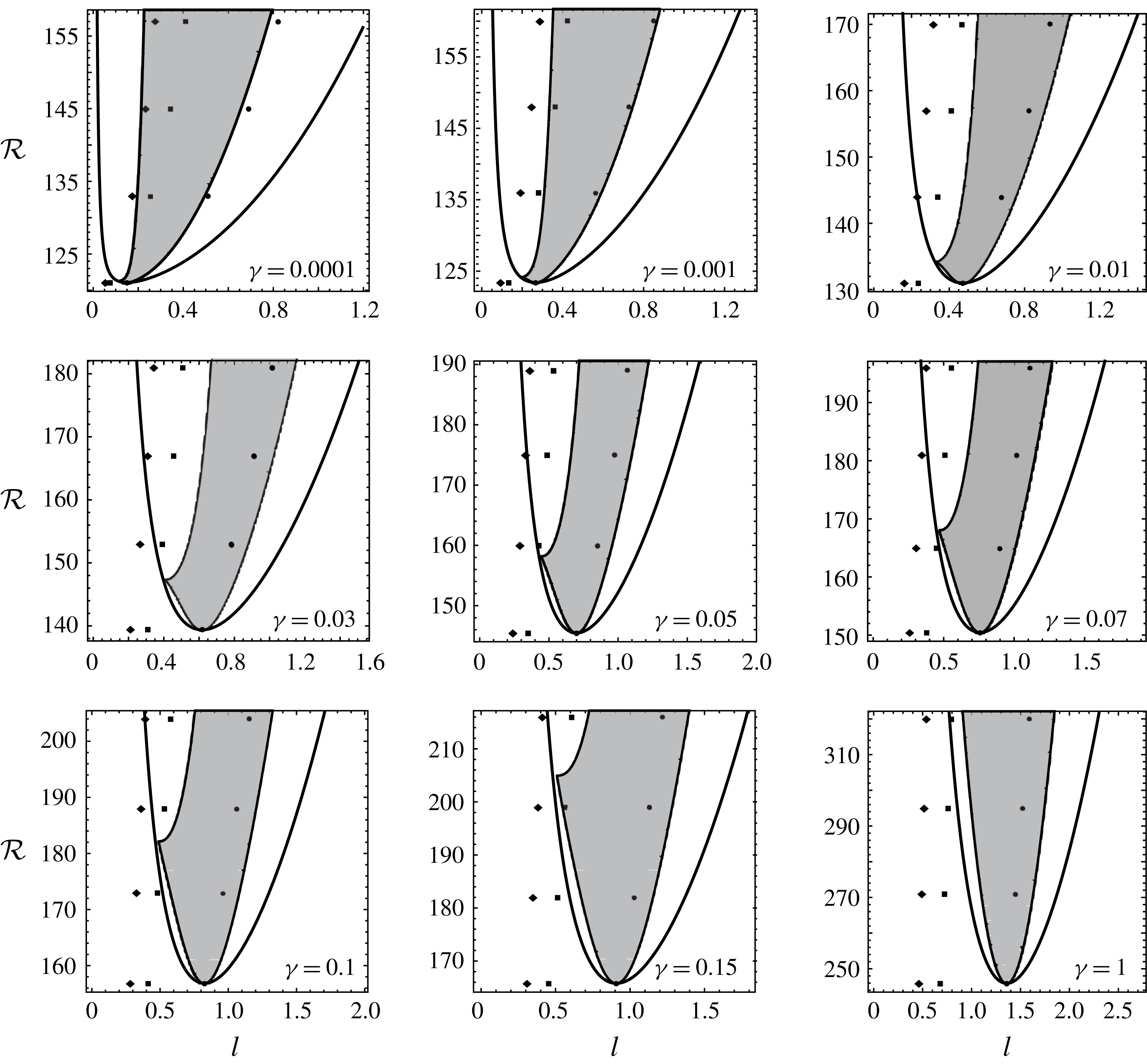
Neutral curves for various
 $\unicode[STIX]{x1D6FE}$
. The solid dots, squares and diamonds plotted at
 ${\mathcal{R}}={\mathcal{R}}_{c}$
,
 $1.1{\mathcal{R}}_{c}$
,
 $1.2{\mathcal{R}}_{c}$
and
 $1.3{\mathcal{R}}_{c}$
reflect the point of maximum growth rate of the fundamental and its
 $1/2$
and
 $1/3$
subharmonics. Note that
 ${\mathcal{R}}_{c}$
varies with
 $\unicode[STIX]{x1D6FE}$
as shown in figure 2. Eckhaus-stable regions discussed in § 4.1 are highlighted in grey.


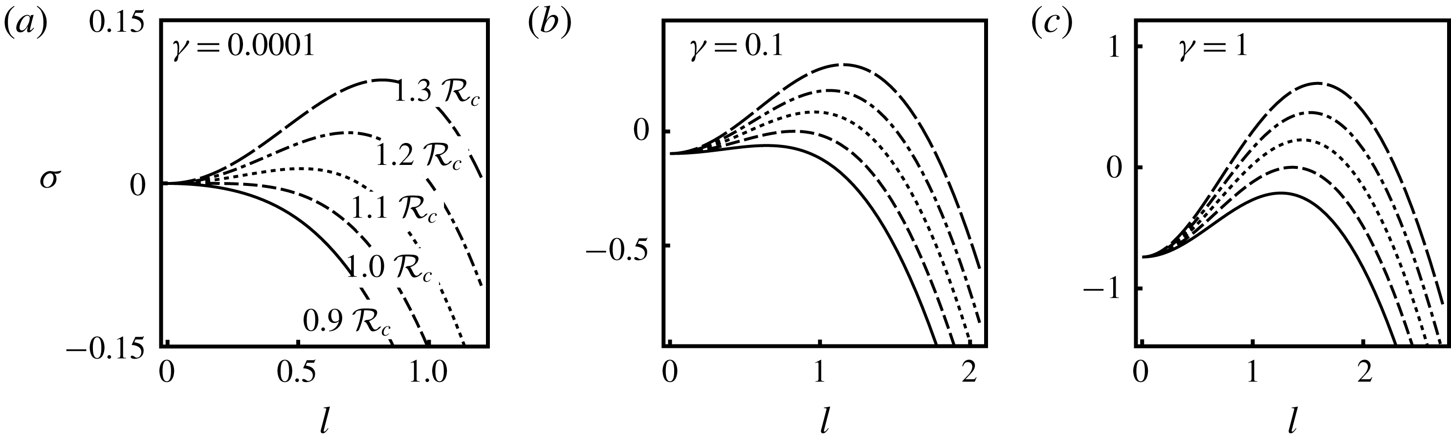
Profiles of growth rate for three values of
 $\unicode[STIX]{x1D6FE}\in (0,1]$
at various values of
 ${\mathcal{R}}$
ranging from
 ${\mathcal{R}}=0.9{\mathcal{R}}_{c}$
to
 ${\mathcal{R}}=1.3{\mathcal{R}}_{c}$
. Note that
 ${\mathcal{R}}_{c}$
varies with
 $\unicode[STIX]{x1D6FE}$
as shown in figure 2.

3.1 Neutral stability curves and growth rate
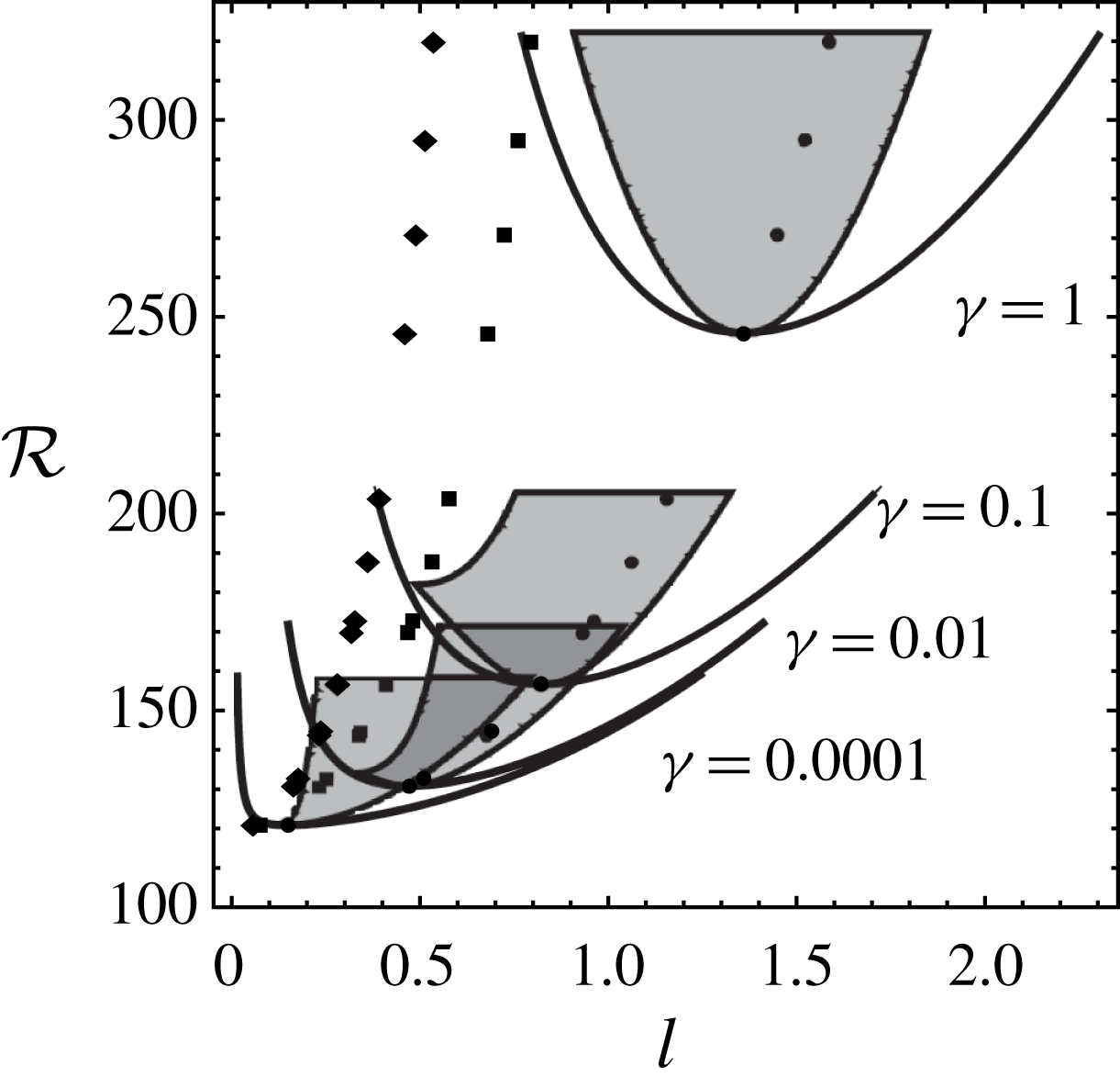
Neutral curves for a range of
 $\unicode[STIX]{x1D6FE}\in (0,1]$
are detailed in figure 1 and for perspective, amalgamated in figure 2. Therein we restrict the plotted range to
 ${\mathcal{R}}\leqslant 1.3{\mathcal{R}}_{c}$
, as it is within these bounds that the nonlinear techniques utilised later are most credible. The maximum growth rates of the fundamental and the
 $1/2$
and
 $1/3$
subharmonics at specific
 ${\mathcal{R}}$
are also included in figures 1 and 2 as solid dots, squares and diamonds. Growth rates at various
 ${\mathcal{R}}$
are provided in figure 3.
Not surprisingly, the generic form of profiles for
 $\unicode[STIX]{x1D6FE}\ll 1$
in figures 1 to 3 are closely in accord with the asymptotic findings of Cox & Leibovich (Reference Cox and Leibovich1993) and Hayes & Phillips (Reference Hayes and Phillips2017). Specifically, that the neutral curve is strongly asymmetric, that the curve of maximum growth rate depicted by dots in figure 1 exhibits an almost linear increase in
 $l$
with
 ${\mathcal{R}}$
and, as we see in figure 3, that
 $\unicode[STIX]{x1D70E}\approx -\unicode[STIX]{x1D6FE}$
at
 $l=0$
for all
 ${\mathcal{R}}$
when
 $\unicode[STIX]{x1D6FE}>0$
(Hayes & Phillips Reference Hayes and Phillips2016, Reference Hayes and Phillips2017).
3.2 The role of
 $\unicode[STIX]{x1D6FE}$
on linear stability

Actually, figure 3 indicates that
 $\unicode[STIX]{x1D6FE}$
acts to suppress instability not only over the smaller wavenumbers but over an increasingly wider range of
 $l$
as
 $\unicode[STIX]{x1D6FE}$
increases; in other words
 $\unicode[STIX]{x1D6FE}$
acts as a low wavenumber cutoff. Perhaps as a consequence of this cutoff, are a series of related features evident in figure 2. First, that the onset values
 $({\mathcal{R}}_{c},l_{c})$
increase from
 $(120,0)$
to approximately
 $(240,1.4)$
as
 $\unicode[STIX]{x1D6FE}$
increases from zero to unity. Second, that the peak growth rate and its accompanying wavenumber likewise increase. Third, that the profile of the neutral curve evolves from strongly asymmetric near the turning point when
 $\unicode[STIX]{x1D6FE}\ll 1$
to almost symmetric as
 $\unicode[STIX]{x1D6FE}\rightarrow 1$
, a feature that has implications in regard to details of the Ginzburg–Landau equation we will discuss in § 4. And fourth, that the neutral curve narrows markedly, causing some subharmonic modes to reside outside of it.
The Biot number
 $\unicode[STIX]{x1D6FE}$
is a measure of the extra stress at the free surface that results not only from the perturbed motion there but also through rectified wave–wave interaction (Longuet-Higgins Reference Longuet-Higgins1953). Irrespective of its origins, however, we need an estimate for
 $\unicode[STIX]{x1D6FE}$
, the first being
 $\unicode[STIX]{x1D6FE}\approx 0.06$
by Cox & Leibovich (Reference Cox and Leibovich1993), based on physical arguments. Phillips & Dai (Reference Phillips and Dai2014), on the other hand, show formally that
 $\unicode[STIX]{x1D6FE}$
may range from an upper bound of unity down to near zero; the latter being utilised in asymptotic studies to isolate the role of
 $\unicode[STIX]{x1D6FE}$
in the limit
 $\unicode[STIX]{x1D6FE}\rightarrow 0$
(Hayes & Phillips Reference Hayes and Phillips2016, Reference Hayes and Phillips2017). In view of this broad variation we proceed as follows: in much of our study (§§ 4–6), we assume a ‘typical’ value to gain insight into the key dynamical features. The typical value we choose is
 $\unicode[STIX]{x1D6FE}=0.03$
. This was not a physical choice but rather a value that captured the gamut of features observed as we investigated a broader range. That broader range, specifically from
 $\unicode[STIX]{x1D6FE}=10^{-4}$
to unity, is reflected in figures 1, 2 and 3 and discussed in § 7.
3.3 Eigenfunctions and adjoint eigenfunctions
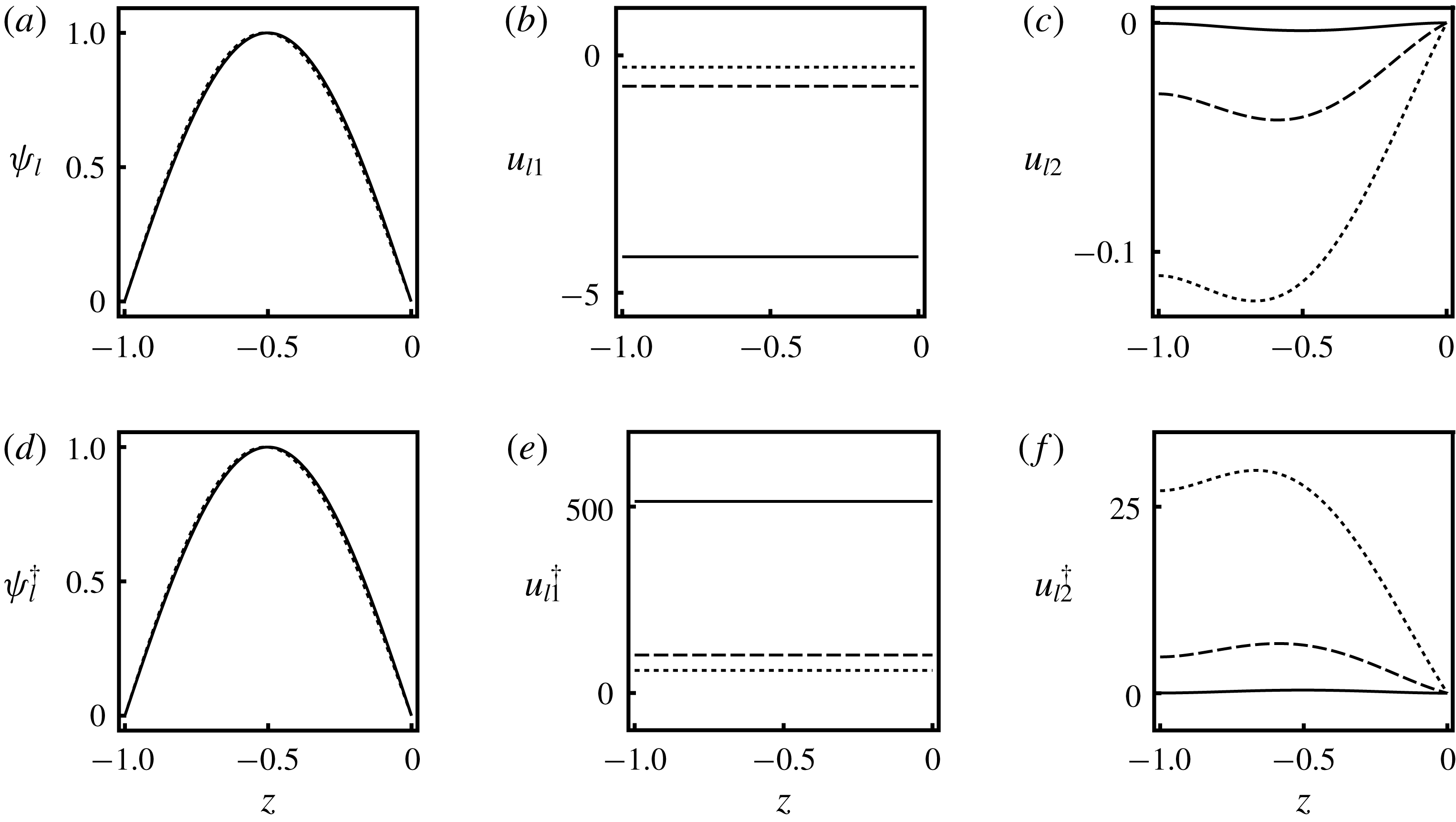
The eigenfunctions
 $\unicode[STIX]{x1D713}_{l}$
and
 $u_{l}$
at the wavenumber of maximum growth rate change little from
 ${\mathcal{R}}_{c}$
to
 $1.3{\mathcal{R}}_{c}$
and so only those at
 ${\mathcal{R}}_{c}$
and
 $l_{c}$
are plotted in figure 4. First, observe that
 $\unicode[STIX]{x1D713}_{l}$
has a sole peak, which means that individual LC fill the layer
 $z\in [-1,0]$
. Second, in spite of top–bottom symmetry being broken by
 $\unicode[STIX]{x1D6FE}$
, the eigenfunction
 $\unicode[STIX]{x1D713}_{l}$
is almost symmetric about the mid-plane (
 $z=-0.5$
). In fact there is little variation with
 $\unicode[STIX]{x1D6FE}$
at all, which indicates that the
 $\unicode[STIX]{x1D6FE}\unicode[STIX]{x1D713}_{l}^{\prime }$
term in (3.4b
) has little influence on the cross-stream flow.
Linear eigenfunctions
 $\unicode[STIX]{x1D713}_{l}$
,
 $u_{l1}$
and
 $u_{l2}$
(a–c) and adjoint linear eigenfunctions
 $\unicode[STIX]{x1D713}_{l}^{\dagger }$
,
 $u_{l1}^{\dagger }$
and
 $u_{l2}^{\dagger }$
(d–f) at
 ${\mathcal{R}}_{c}$
for several values of
 $\unicode[STIX]{x1D6FE}$
, viz:
 $\unicode[STIX]{x1D6FE}=10^{-4}$
solid line;
 $\unicode[STIX]{x1D6FE}=0.1$
dashed line; and
 $\unicode[STIX]{x1D6FE}=1$
dotted line.

In contrast, the streamwise perturbations
 $u_{l}$
show clear variations with
 $\unicode[STIX]{x1D6FE}$
and may be decomposed into a constant offset and a
 $z$
-varying part,
 $u_{l1}$
and
 $u_{l2}$
say, the former by far the larger. Such decompositions are not uncommon in vortex wave interaction problems (Hall & Smith Reference Hall and Smith1988; Phillips Reference Phillips, Debnath and Riahi1998b
; Hayes & Phillips Reference Hayes and Phillips2017). We quantify the parts by requiring
 $u_{l2}(0)=0$
and normalise them by a factor that ensures
 $\unicode[STIX]{x1D713}_{l}$
is unity normalised. Then, as
 $\unicode[STIX]{x1D6FE}$
increases, it is evident that
 $|u_{l1}|$
falls rapidly while
 $|u_{l2}|$
slowly increases. Moreover
 $u_{l2}$
evolves from symmetric in the limit
 $\unicode[STIX]{x1D6FE}\rightarrow 0$
(see figure 6 of Hayes & Phillips (Reference Hayes and Phillips2017)) to asymmetric at larger
 $\unicode[STIX]{x1D6FE}$
, in accord with the gradual breaking of top–bottom symmetry in the boundary condition (3.4a
) as
 $\unicode[STIX]{x1D6FE}$
increases.
We solve the linear adjoint problem to (3.3) by entirely similar numerical methods and find that the adjoint eigenfunction
 $\unicode[STIX]{x1D713}_{l}^{\dagger }(z)$
is indistinguishable from
 $\unicode[STIX]{x1D713}_{l}$
, as we see in the lower row of figure 4. Accordingly, we likewise pare the adjoint eigenfunction
 $u_{l}^{\dagger }$
into an offset
 $u_{l1}^{\dagger }$
and asymmetric part
 $u_{l2}^{\dagger }$
that together are two orders of magnitude larger than
 $\unicode[STIX]{x1D713}_{l}^{\dagger }$
. Not unexpectedly the adjoint eigenfunctions mimic their regular counterparts.
4 Nonlinear dynamics of single modes
Nonlinearities ultimately curb the exponential growth defined by (3.1) and our goal now is to determine their role by analysing the complete CL equations (2.2). We begin with restrictions. Specifically, we first restrict our attention to the study of isolated modes, i.e. relative to a fundamental mode of spanwise wavenumber
 $l$
, defined as the least stable linear mode, we permit the excitation of harmonic modes, but exclude their interaction. Our plan is to explore such excitation via an Eckhaus instability analysis of a Ginzburg–Landau (GL) like equation (Ginzburg & Landau Reference Ginzburg and Landau1950; Newell & Whitehead Reference Newell and Whitehead1969) built upon the CL equations, via a multiple scale approach. That said, the devil of multi-parameter expansions is in their detail and for that reason we proceed in stages, beginning in the asymptotic limit
 $\unicode[STIX]{x1D6FE}\rightarrow 0$
, where the detail can be precisely determined.
4.1 A long wave approach
To that end we defer to a construct with
 $D^{\prime }=U^{\prime }=1$
employed by Cox & Leibovich (Reference Cox and Leibovich1993) to elicit the role of
 $\unicode[STIX]{x1D6FE}$
in the limit
 $\unicode[STIX]{x1D6FE}\rightarrow 0$
(see § 3.2). As a part of that study, they derive an asymptotically reduced partial differential equation (PDE) from (2.2b,c
) with (2.4) for the depth-averaged streamwise velocity perturbation. Of note is that their reduced PDE, which is derived in more detail in Cox & Leibovich (Reference Cox and Leibovich1994), is not the result of a weakly nonlinear analysis, but rather relies on a long wavelength (in
 $y$
) expansion that allows the coefficients premultiplying each term in the PDE to be precisely determined. As our starting point, therefore, we first derive the GL equation from their PDE, which in the absence of stratification and in the long wave limit, has the form (Cox & Leibovich Reference Cox and Leibovich1993, Reference Cox and Leibovich1994)
 $$\begin{eqnarray}\displaystyle \mathfrak{u}_{t}=-\unicode[STIX]{x1D6FE}\mathfrak{u}-r^{\ast }\mathfrak{u}_{yy}-p\mathfrak{u}_{yyyy}+q(\mathfrak{u}_{y})_{y}^{3}, & & \displaystyle\end{eqnarray}$$
where
 $\mathfrak{u}$
is the depth averaged value of
 $u$
across the layer, with
 $$\begin{eqnarray}\displaystyle r^{\ast }=\frac{{\mathcal{R}}-{\mathcal{R}}_{0}}{{\mathcal{R}}_{0}},\quad p=\frac{1091}{5544},\quad q=\frac{155}{126}\quad \text{and}\quad {\mathcal{R}}_{0}=120. & & \displaystyle\end{eqnarray}$$
We note that (4.1) is strictly asymptotically consistent, with
 $\unicode[STIX]{x1D6FE}=O(l^{4})$
,
 $r^{\ast }=O(l^{2})$
,
 $\unicode[STIX]{x2202}_{y}=O(l)$
,
 $\unicode[STIX]{x2202}_{t}=O(l^{4})$
and
 $p,q=O(1)$
as
 $l\rightarrow 0$
.
On assuming linear solutions proportional to
 $\text{e}^{\unicode[STIX]{x1D70E}t+\text{i}ly}$
, the dispersion relationship
 $$\begin{eqnarray}\displaystyle \unicode[STIX]{x1D70E}=-\unicode[STIX]{x1D6FE}+r^{\ast }l^{2}-pl^{4} & & \displaystyle\end{eqnarray}$$
and neutral curve
 $$\begin{eqnarray}\displaystyle {\mathcal{R}}={\mathcal{R}}_{0}\left(1+\frac{\unicode[STIX]{x1D6FE}}{l^{2}}\right)+l^{2}p{\mathcal{R}}_{0} & & \displaystyle\end{eqnarray}$$
readily follow from (4.1) and concur with previous work (Cox & Leibovich Reference Cox and Leibovich1993; Hayes & Phillips Reference Hayes and Phillips2016). Moreover, since
 $l_{c}=(\unicode[STIX]{x1D6FE}/p)^{1/4}$
, then
 $l_{c}\rightarrow 0$
as
 $\unicode[STIX]{x1D6FE}\rightarrow 0$
, which together indicate that (4.4) is strongly asymmetric about
 $l_{c}$
.
Our task now is to derive a GL equation from (4.1). To that end we make the ansatz
 $$\begin{eqnarray}\displaystyle \mathfrak{u}(y,t;l,\unicode[STIX]{x1D700})=\mathfrak{U}({\hat{y}},Y,\hat{t},T;l,\unicode[STIX]{x1D700})\sim \unicode[STIX]{x1D700}\mathfrak{u}_{1} & & \displaystyle\end{eqnarray}$$
and introduce scaling consistent with that employed by Cox & Leibovich (Reference Cox and Leibovich1994) in the derivation of (4.1), viz.
 $\unicode[STIX]{x2202}_{y}=l(\unicode[STIX]{x2202}_{{\hat{y}}}+\unicode[STIX]{x1D700}\unicode[STIX]{x2202}_{Y})$
,
 $\unicode[STIX]{x2202}_{t}=l^{4}(\unicode[STIX]{x2202}_{\hat{t}}+\unicode[STIX]{x1D700}^{2}\unicode[STIX]{x2202}_{T})$
and
 $\unicode[STIX]{x1D6FE}\equiv l^{4}\hat{\unicode[STIX]{x1D6FE}}$
, with
 $r^{\ast }\equiv l^{2}\hat{r}\sim l^{2}(\hat{r}_{c}+\unicode[STIX]{x1D700}^{2}\hat{\unicode[STIX]{x1D706}})$
. Here
 $\hat{\unicode[STIX]{x1D6FE}}$
,
 $\hat{r}_{c}$
and
 $\hat{\unicode[STIX]{x1D706}}$
are
 $O(1)$
and
 $\unicode[STIX]{x1D700}^{2}=({\mathcal{R}}-{\mathcal{R}}_{c})/{\mathcal{R}}_{c}$
. Then on substituting into (4.1), collecting terms at like order in
 $\unicode[STIX]{x1D700}$
and cancelling common factors of the small parameter
 $l$
, yields at
 $O(\unicode[STIX]{x1D700})$
that
 $$\begin{eqnarray}\displaystyle \mathfrak{u}_{1}=A(Y,T)\text{e}^{\text{i}\hat{l}_{c}{\hat{y}}}+\text{c.c.} & & \displaystyle\end{eqnarray}$$
Herein
 $A$
is an unknown slowly varying amplitude that is a function of the slow spatial and temporal scales,
 $Y$
and
 $T$
, while the fast spatial scale
 ${\hat{y}}$
is taken relative to
 $l_{c}$
, here denoted
 $\hat{l}_{c}$
because
 $\hat{l}_{c}{\hat{y}}$
is
 $O(1)$
. Proceeding then to higher order, we find at
 $O(\unicode[STIX]{x1D700}^{2})$
that
 $\hat{r}_{c}=2p\hat{l}_{c}^{2}$
and realise, at
 $O(\unicode[STIX]{x1D700}^{3})$
, the strictly asymptotically consistent GL equation
 $$\begin{eqnarray}\displaystyle A_{T}=\hat{\unicode[STIX]{x1D70E}}A+\hat{\unicode[STIX]{x1D6FD}}_{32}A_{YY}+\hat{\unicode[STIX]{x1D6FD}}_{31}|A|^{2}A & & \displaystyle\end{eqnarray}$$
with precisely defined
 $O(1)$
coefficients
 $$\begin{eqnarray}\displaystyle \hat{\unicode[STIX]{x1D70E}}=\hat{\unicode[STIX]{x1D706}}\hat{l}_{c}^{2},\quad \hat{\unicode[STIX]{x1D6FD}}_{32}=4p\hat{l}_{c}^{2},\quad \hat{\unicode[STIX]{x1D6FD}}_{31}=-3q\hat{l}_{c}^{4}. & & \displaystyle\end{eqnarray}$$
4.2 Reconstitution
In contrast, we cannot determine whether the GL equation is strictly asymptotically consistent if we instead derive it via reconstitution. That can be important, because the absence of asymptotic consistency can lead to spurious dynamics, especially when triggered by onset growth rates with non-zero imaginary parts (Knobloch & Luca Reference Knobloch and Luca1990). Our growth rates, however, are purely real and since we must necessarily employ reconstitution to derive a GL equation valid over
 $\unicode[STIX]{x1D700}\in [0,0.5)$
and
 $\unicode[STIX]{x1D6FE}\in (0,1]$
, it is instructive to determine first whether reconstitution yields results consistent with those in § 4.1.
To that end we assume that the lead term in the expansion
 $$\begin{eqnarray}\displaystyle \mathfrak{u}=\unicode[STIX]{x1D700}^{j}\mathfrak{u}_{j}\quad (j=1,4) & & \displaystyle\end{eqnarray}$$
for weakly nonlinear solutions to (4.1) is captured by the ansatz
 $$\begin{eqnarray}\displaystyle \mathfrak{u}_{1}=A(Y,T_{1},T_{2},T_{3})\text{e}^{(\unicode[STIX]{x1D70E}\hat{t}+\text{i}l{\hat{y}})} & & \displaystyle\end{eqnarray}$$
in accord with the multi-scale expansion outlined by Suslov & Paolucci (Reference Suslov and Paolucci2004), viz.
 $\unicode[STIX]{x2202}_{y}=\unicode[STIX]{x2202}_{{\hat{y}}}+\unicode[STIX]{x1D700}\unicode[STIX]{x2202}_{Y}$
as above, but now with
 $\unicode[STIX]{x2202}_{t}=\unicode[STIX]{x2202}_{\hat{t}}+\unicode[STIX]{x1D700}^{j}\unicode[STIX]{x2202}_{T_{j}}$
. Concordant with
 $r^{\ast }$
in § 4.1, and at fixed
 $\unicode[STIX]{x1D700}^{2}$
, we then write
 $$\begin{eqnarray}\displaystyle r^{\ast }\equiv \left(\frac{{\mathcal{R}}_{c}-{\mathcal{R}}_{0}}{{\mathcal{R}}_{0}}\right)+\unicode[STIX]{x1D700}^{2}\left(\frac{{\mathcal{R}}-{\mathcal{R}}_{c}}{{\mathcal{R}}_{0}}\right)=r_{c}^{\ast }+\unicode[STIX]{x1D700}^{2}\unicode[STIX]{x1D706}^{\ast }. & & \displaystyle\end{eqnarray}$$
We then substitute (4.9)–(4.11) into (4.1) and solve at successive orders in
 $\unicode[STIX]{x1D700}$
.
First, we find at
 $O(\unicode[STIX]{x1D700}^{2})$
that
 $A_{T_{1}}=0$
and thus that
 $A_{T}$
reduces to
 $A_{T}=A_{T_{2}}+\unicode[STIX]{x1D700}A_{T_{3}}+\cdots \,$
. Then, at
 $O(\unicode[STIX]{x1D700}^{3})$
, we see that
 $A_{T_{2}}$
not only concurs with (4.7), but has coefficients
 $$\begin{eqnarray}\displaystyle \unicode[STIX]{x1D70E}=\unicode[STIX]{x1D706}^{\ast }l^{2},\quad \unicode[STIX]{x1D6FD}_{32}=4pl^{2}\quad \text{and}\quad \unicode[STIX]{x1D6FD}_{31}=-3ql^{4} & & \displaystyle\end{eqnarray}$$
in accord with (4.8). Finally,
 $A_{T_{3}}$
is given at
 $O(\unicode[STIX]{x1D700}^{4})$
with the additional coefficients
 $$\begin{eqnarray}\displaystyle \unicode[STIX]{x1D6FD}_{21}=-2\unicode[STIX]{x1D700}\unicode[STIX]{x1D706}^{\ast }l,\quad \unicode[STIX]{x1D6FD}_{43}=-4\unicode[STIX]{x1D700}pl,\quad \unicode[STIX]{x1D6FD}_{41}=12\unicode[STIX]{x1D700}ql^{3}. & & \displaystyle\end{eqnarray}$$
Correct to
 $O(\unicode[STIX]{x1D700}^{4})$
, the reconstituted GL equation is then
 $$\begin{eqnarray}\displaystyle A_{T}=\unicode[STIX]{x1D70E}A+\unicode[STIX]{x1D6FD}_{32}A_{YY}+\unicode[STIX]{x1D6FD}_{31}A|A|^{2}+\text{i}\unicode[STIX]{x1D6FD}_{21}A_{Y}+\text{i}\unicode[STIX]{x1D6FD}_{43}A_{YYY}+\text{i}\unicode[STIX]{x1D6FD}_{41}|A|^{2}A_{Y}. & & \displaystyle\end{eqnarray}$$
But why go to
 $O(\unicode[STIX]{x1D700}^{4})$
when we know that (4.14) must reduce to (4.7) in the limit
 $\unicode[STIX]{x1D700}\rightarrow 0$
and know that the GL equation at
 $O(\unicode[STIX]{x1D700}^{3})$
is adequate when the bifurcation is supercritical as it is here? To see why we first note that the coefficients are evaluated at
 $l=l_{c}=(\unicode[STIX]{x1D6FE}/p)^{1/4}$
and thus vary with
 $\unicode[STIX]{x1D6FE}$
as
 $$\begin{eqnarray}\displaystyle \unicode[STIX]{x1D70E}=\unicode[STIX]{x1D706}^{\ast }\left(\frac{\unicode[STIX]{x1D6FE}}{p}\right)^{1/2},\quad \unicode[STIX]{x1D6FD}_{32}=4p\left(\frac{\unicode[STIX]{x1D6FE}}{p}\right)^{1/2},\quad \unicode[STIX]{x1D6FD}_{31}=-\frac{3q\unicode[STIX]{x1D6FE}}{p}, & & \displaystyle\end{eqnarray}$$
with
 $$\begin{eqnarray}\displaystyle \unicode[STIX]{x1D6FD}_{21}=-2\unicode[STIX]{x1D700}\unicode[STIX]{x1D706}^{\ast }\left(\frac{\unicode[STIX]{x1D6FE}}{p}\right)^{1/4},\quad \unicode[STIX]{x1D6FD}_{43}=-4\unicode[STIX]{x1D700}p\left(\frac{\unicode[STIX]{x1D6FE}}{p}\right)^{1/4},\quad \unicode[STIX]{x1D6FD}_{41}=12\unicode[STIX]{x1D700}q\left(\frac{\unicode[STIX]{x1D6FE}}{p}\right)^{3/4},\qquad & & \displaystyle\end{eqnarray}$$
which means their relative importance must be explored not just as
 $\unicode[STIX]{x1D700}\rightarrow 0$
, but rather in the double limit
 $\unicode[STIX]{x1D700},\unicode[STIX]{x1D6FE}\rightarrow 0$
. For example, consider the limit
 $\unicode[STIX]{x1D6FD}_{43}/\unicode[STIX]{x1D6FD}_{32}\sim -\unicode[STIX]{x1D700}(\unicode[STIX]{x1D6FE}/p)^{-1/4}=s$
say, as
 $\unicode[STIX]{x1D700},\unicode[STIX]{x1D6FE}\rightarrow 0$
. Of course
 $s$
does vanish as we expect but only if the limits satisfy
 $\unicode[STIX]{x1D700}\ll (\unicode[STIX]{x1D6FE}/p)^{1/4}$
; in contrast
 $s=O(1)$
once
 $\unicode[STIX]{x1D700}=O(\unicode[STIX]{x1D6FE}^{1/4})$
. We should not forget that
 $\unicode[STIX]{x1D6FE}$
is itself small, but the fact remains that (4.14) reduces to (4.7) only for levels of supercriticality
 $\unicode[STIX]{x1D700}$
significantly smaller than
 $O(\unicode[STIX]{x1D6FE}^{1/4})$
, which in consequence implies that there is a level of supercriticality above which terms premultiplied by
 $\unicode[STIX]{x1D6FD}_{21}$
and
 $\unicode[STIX]{x1D6FD}_{43}$
must be retained. Put differently, although (4.7) is strictly asymptotically consistent in
 $\unicode[STIX]{x1D700}$
, its range of validity is affected by
 $\unicode[STIX]{x1D6FE}$
and restricted, as
 $\unicode[STIX]{x1D6FE}$
decreases, to ever smaller values of
 $\unicode[STIX]{x1D700}$
from the critical, evidencing a non-uniformity not present in (4.14).
This finding is particularly important when we perform an Eckhaus-type instability analysis. Therein we examine the nonlinear stability of (4.7) or (4.14) to a wave solution of the form
 $$\begin{eqnarray}\displaystyle A(Y,T)={\mathcal{M}}\text{e}^{\text{i}\unicode[STIX]{x1D714}T}\text{e}^{\text{i}kY}, & & \displaystyle\end{eqnarray}$$
in which
 ${\mathcal{M}}$
is the magnitude of the wave and
 $k$
is defined as
 $k=(l-l_{c})$
with frequency
 $\unicode[STIX]{x1D714}$
. More precisely, we seek a stationary wave solution that is stable to perturbations (Doelman & Eckhaus Reference Doelman and Eckhaus1991). Of interest is the dispersion relationship defined by the linear steady states
 $A_{T}=0$
, determined by the substitution of (4.16) with
 $\unicode[STIX]{x1D714}=0$
into (4.7), yielding
 $\unicode[STIX]{x1D70E}=k^{2}\unicode[STIX]{x1D6FD}_{32}$
or into (4.14), giving
 $$\begin{eqnarray}\displaystyle \unicode[STIX]{x1D70E}=k\unicode[STIX]{x1D6FD}_{21}+k^{2}\unicode[STIX]{x1D6FD}_{32}-k^{3}\unicode[STIX]{x1D6FD}_{43}. & & \displaystyle\end{eqnarray}$$
Looking first to the expression for (4.7) we see that the growth rate is parabolic in
 $l$
about
 $l_{c}$
as we expect. However, if we note from (4.15) (see also table 1) that
 $\unicode[STIX]{x1D70E}$
is proportional to
 $\unicode[STIX]{x1D706}^{\ast }$
and express
 $\unicode[STIX]{x1D706}^{\ast }\propto k^{2}\unicode[STIX]{x1D6FD}_{32}$
in terms of
 ${\mathcal{R}}(l)$
, we find that the curve lies inside the linear neutral curve (4.4) over
 $l\geqslant l_{c}$
as expected, but protrudes through and lies outside of (4.4) for some
 $l<l_{c}$
, which is unexpected. This violation occurs at values of
 $\unicode[STIX]{x1D700}$
consistent with those mentioned above and highlights limitations on the level of supercriticality over which the cubic GL equation remains viable. Of course this could be an artefact associated with weakly nonlinear stripe solutions of the form (4.16), but since we know the cubic GL equation is non-uniform in
 $\unicode[STIX]{x1D700}$
, we turn instead to the quartic-order GL equation (4.14) and subject it to the same test. Specifically, on noting that
 $\unicode[STIX]{x1D6FD}_{21}\propto \unicode[STIX]{x1D706}^{\ast }$
from (4.15) and now expressing (4.17) in terms of
 ${\mathcal{R}}$
, the curve
 ${\mathcal{R}}(l)$
for the linear steady states
 $A_{T}=0$
is found to live entirely within the linearly unstable region of (4.4), mimics it as it should, and osculates to it at the critical point as it must.


4.3 Ginzburg–Landau equation from the CL equation
Our intent now is to derive an amplitude equation of GL type that describes the evolution of
 $A(Y,T)$
by employing the methods of multiple scales outlined by Suslov & Paolucci (Reference Suslov and Paolucci2004) valid over a range of
 $\unicode[STIX]{x1D700}$
and
 $\unicode[STIX]{x1D6FE}$
. As in § 4.2, we restrict attention to nonlinearities that are sufficiently weak that semi-analytical methods can be applied to study them. Such restrictions are commensurate with the ansatz (Cox et al.
Reference Cox, Leibovich, Moroz and Tandon1992b
)
 $$\begin{eqnarray}\displaystyle \left(\begin{array}{@{}c@{}}u\\ \unicode[STIX]{x1D713}\end{array}\right)=\left(\begin{array}{@{}c@{}}A(Y,T)u_{l}(z)\text{e}^{\text{i}ly}\\ A(Y,T)\unicode[STIX]{x1D713}_{l}(z)\text{e}^{\text{i}ly}\end{array}\right)+\text{c.c.} & & \displaystyle\end{eqnarray}$$
Again,
 $A(Y,T)$
is an unknown slowly varying amplitude that is a function of spatial and temporal scales
 $Y$
and
 $T$
that, in terms of the small parameter
 $\unicode[STIX]{x1D700}$
and relative to the ‘fast’ scales
 ${\hat{y}}$
and
 $\hat{t}$
, vary gradually as
 $\unicode[STIX]{x2202}_{y}=\unicode[STIX]{x2202}_{{\hat{y}}}+\unicode[STIX]{x1D700}\unicode[STIX]{x2202}_{Y}$
and
 $\unicode[STIX]{x2202}_{t}=\unicode[STIX]{x2202}_{\hat{t}}+\unicode[STIX]{x1D700}\unicode[STIX]{x2202}_{T}$
. That said, we find for asymptotic consistency when the control parameter
 ${\mathcal{R}}$
is not much greater than
 ${\mathcal{R}}_{c}$
(
 $\unicode[STIX]{x1D700}\ll 1$
) that the slow time scale corresponds to
 $\unicode[STIX]{x1D70E}^{-1}$
.
On substituting (4.18) into (2.2b,c
), we quickly find that higher-order contributions to
 $Y$
play little role in the dispersion relationship and so do not expand
 $Y$
further, but we do expand
 $T$
as
 $T_{j}=\unicode[STIX]{x1D700}^{j}t$
so that
 $\unicode[STIX]{x1D700}\unicode[STIX]{x2202}_{T}=\unicode[STIX]{x1D700}^{j}\unicode[STIX]{x2202}_{T_{j}}$
. We then solve for
 $A_{T_{j}}$
at successively higher orders in
 $\unicode[STIX]{x1D700}$
, progressively reconstituting the results at each order to determine
 $A_{T}$
. For reasons discussed in § 4.2, we truncate the GL equation at
 $O(\unicode[STIX]{x1D700}^{4})$
rather than third order. The ensuing GL equation is again given by (4.14) in which, as above,
 $\unicode[STIX]{x1D6FD}_{ij}$
are real coefficients and the
 $Y\rightarrow -Y$
symmetry is broken by the terms
 $A_{Y}$
,
 $|A|^{2}A_{Y}$
and
 $A_{YYY}$
. Here too all terms of a certain order of smallness in
 $\unicode[STIX]{x1D700}$
have been retained, rendering the construction of (4.14) systematic, but not strictly asymptotic in the sense that all terms arise at the same asymptotic order in
 $\unicode[STIX]{x1D700}$
as in § 4.1.
Since the derivation is straightforward we will not discuss it further, but it is useful to outline the systematic process akin to that employed in § 4.2 utilised to ensure the coefficients are of consistent order. We begin with the coefficient premultiplying the cubic nonlinearity at the heart of the GL equation,
 $\unicode[STIX]{x1D6FD}_{31}A|A|^{2}$
, and compare it with
 $\unicode[STIX]{x1D6FD}_{32}$
premultiplying
 $A_{YY}$
that also arises at
 $O(\unicode[STIX]{x1D700}^{3})$
. The question is whether the term
 $\unicode[STIX]{x1D6FD}_{32}A_{YY}$
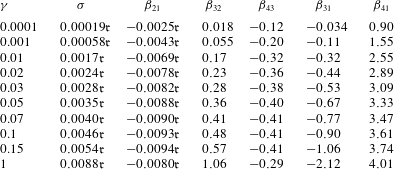
should be retained and we decide yes because, from table 1,
 $|\unicode[STIX]{x1D6FD}_{32}/\unicode[STIX]{x1D6FD}_{31}|=O(1)$
for all
 $\unicode[STIX]{x1D6FE}$
. Cubic nonlinearities also arise at
 $O(\unicode[STIX]{x1D700}^{4})$
through
 $\text{i}\unicode[STIX]{x1D6FD}_{41}|A|^{2}A_{Y}$
and we next question whether they too are of comparable order to
 $\unicode[STIX]{x1D6FD}_{31}A|A|^{2}$
. For that to be so necessitates
 $\unicode[STIX]{x1D700}|\unicode[STIX]{x1D6FD}_{41}/\unicode[STIX]{x1D6FD}_{31}|=O(1)$
over some
 $\unicode[STIX]{x1D700}\in (0,0.5)$
at each
 $\unicode[STIX]{x1D6FE}$
, which from table 1, is indeed the case.
Coefficients in the quartic Ginzburg–Landau equation (4.14) derived from Cox & Leibovich’s (Reference Cox and Leibovich1993) asymptotically reduced (4.1) long wave version of (2.2) and defined in (4.12), and numerically evaluated values from the generalised version described in § 4.3. Results are evaluated at the critical points for
 $\unicode[STIX]{x1D6FE}=0.0001$
with
 $\mathfrak{r}={\mathcal{R}}-{\mathcal{R}}_{c}$
.

Turning now to the linear terms we impose two requirements: the first being that at successive orders
 $O(\unicode[STIX]{x1D700}^{j})$
for
 $j=2,3,4$
each coefficient satisfies
 $\unicode[STIX]{x1D700}^{j-1}|\unicode[STIX]{x1D6FD}_{jj-1}|/\unicode[STIX]{x1D70E}^{\ast }=O(1)$
(no sum) where
 $\unicode[STIX]{x1D70E}=\mathfrak{r}\unicode[STIX]{x1D70E}^{\ast }$
and the second being that the linear terms together act to recover the asymmetric behaviour depicted in the neutral curve. Looking first at the coefficients at
 $O(\unicode[STIX]{x1D700}^{2})$
, we find from table 1 that
 $\unicode[STIX]{x1D700}|\unicode[STIX]{x1D6FD}_{21}|/\unicode[STIX]{x1D70E}^{\ast }$
diminishes as
 $\unicode[STIX]{x1D6FE}$
increases, but is
 $O(1)$
for
 $\unicode[STIX]{x1D6FE}<0.15$
. In contrast at
 $O(\unicode[STIX]{x1D700}^{3})$
, the ratio
 $\unicode[STIX]{x1D700}^{2}\unicode[STIX]{x1D6FD}_{32}/\unicode[STIX]{x1D70E}^{\ast }=O(1)$
for all
 $\unicode[STIX]{x1D6FE}$
. Finally at
 $O(\unicode[STIX]{x1D700}^{4})$
and as
 $\unicode[STIX]{x1D6FE}$
increases, the ratio
 $\unicode[STIX]{x1D700}^{3}|\unicode[STIX]{x1D6FD}_{43}|/\unicode[STIX]{x1D70E}^{\ast }$
diminishes from
 $O(1)$
to
 $O(\unicode[STIX]{x1D700})$
. Phrased differently, while the symmetric term
 $\unicode[STIX]{x1D6FD}_{32}A_{YY}$
plays a role at all
 $\unicode[STIX]{x1D6FE}$
, the symmetry-breaking terms
 $\text{i}\unicode[STIX]{x1D6FD}_{21}A_{Y}$
and
 $\text{i}\unicode[STIX]{x1D6FD}_{43}A_{YYY}$
do not. Rather their role diminishes as
 $\unicode[STIX]{x1D6FE}$
increases, in accord with the topology of the neutral stability curve (see figure 1), which becomes progressively more symmetric.
Finally, we compare the coefficients derived directly from (2.2) with their counterparts derived from the asymptotically reduced version of (2.2). Examples at
 $\unicode[STIX]{x1D6FE}=0.0001$
are listed in table 2. First, we see that
 ${\mathcal{R}}_{c}$
,
 $l_{c}$
and
 $\unicode[STIX]{x1D70E}$
agree closely, as do the coefficients
 $\unicode[STIX]{x1D6FD}_{21}$
,
 $\unicode[STIX]{x1D6FD}_{32}$
and
 $\unicode[STIX]{x1D6FD}_{43}$
that premultiply the linear terms. On the other hand the coefficients
 $\unicode[STIX]{x1D6FD}_{31}$
and
 $\unicode[STIX]{x1D6FD}_{41}$
premultiplying the nonlinear terms are vastly different, the generalised coefficients being approximately 18 times larger than the asymptotic ones in (4.15).
4.4 Normalisation, non-uniqueness and distinguished limits
While initially bewildering, such discrepancies are commonplace in weakly nonlinear analysis and are commonly explained by the choice of normalisation and solvability conditions, or the non-uniqueness of equations derived via multi-parameter expansions. We make no attempt to resolve which, or indeed whether a combination of each lead to the discrepancy in nonlinear coefficients here, although we can exclude normalisation, as that was the first thing we checked. For background, however, we will outline the thought patterns behind each possibility.
The first is concerned, in part, with the way the linear eigenfunctions employed in evaluating the coefficients are normalised and in part by the solvability conditions chosen to close the formulation. The consequences of normalisation, which in essence says that the magnitude of the perturbation amplitude cannot be determined from the linear problem is, of course, obvious but solvability requires explanation.
To wit, when (4.18) is substituted into (2.2b,c ) and each order is pared into a left-hand side of unknown variables in terms of a right-hand side of known variables, compatibility between the two sides provides useful information and a carefully chosen inner product even more. But the information is seldom enough to fix on particular values of the system constants. Rather two typical scenarios arise: one being that the system has infinitely many solutions and so a further orthogonality condition must be imposed to fix on a particular one. The second being that the system has a unique solution for any Landau constant, so that we must again invoke an orthogonality condition to fix a particular one. Unfortunately the derivation of (4.1) too has complications, viz. secular terms that depend linearly on the fast time. These, of course, must be avoided and we do so by imposing orthogonality conditions across the layer. Key, however, is that the orthogonality conditions utilise normalised eigenfunctions whose rectified details carry through to the coefficients (4.12). In other words the coefficients in the asymptotically reduced (4.1) are not immune from a projection procedure resulting from an orthogonality condition with respect to a weighted inner product. Because of that, and since different projections can lead to different results, we should not expect our coefficients for the nonlinear terms in (4.14) to concur quantitatively with those in (4.12).
The second explanation, which was articulated by a gracious anonymous referee, has to do with the non-uniqueness of equations derived via multi-parameter expansions, either in terms of
 $\unicode[STIX]{x1D700}$
and
 $l$
or, equivalently,
 ${\mathcal{R}}$
and
 $\unicode[STIX]{x1D6FE}$
in the absence of clearly defined distinguished limits. That is, while the asymptotically reduced (4.1) applies in the limit
 $\unicode[STIX]{x1D6FE}$
and, hence,
 $l\rightarrow 0$
with only mild restrictions on
 ${\mathcal{R}}$
and the modal amplitude, the strictly asymptotically consistent cubic-order GL equation (4.7) follows by taking a further small amplitude limit. In other words, (4.7) results from an analysis corresponding to a distinct path through parameter space, as indeed does our (4.14), however, the paths are different and so too the values of the coefficients premultiplying the nonlinear terms, even though the form of the GL equation remains the same.
4.5 Eckhaus instability
Out task now is to perform an Eckhaus-type instability analysis of (4.14) by examining the nonlinear stability of the stationary wave solution (4.16). We then choose a region in which the solution (4.16) is stable to perturbations (Doelman & Eckhaus Reference Doelman and Eckhaus1991). That region is marked in grey and shown in relation to the neutral curves in figures 1 and 2 for a range
 $\unicode[STIX]{x1D6FE}\in (0,1]$
. The values of the coefficients in (4.14) for selected values of
 $\unicode[STIX]{x1D6FE}$
are given in table 1. Several features are worth noting.
First, the Eckhaus boundary is asymmetric, mimics that of the neutral curve and lies within it. Second, the Eckhaus stability boundaries are neither narrow in the sense that characterise strong pattern selection (Eckhaus & Iooss Reference Eckhaus and Iooss1989), nor wide in the sense that multiple harmonics lie within the boundary. More typically the case here (at least for
 $\unicode[STIX]{x1D6FE}\geqslant 0.001$
see figure 1), is that only the fastest-growing linear modes lie within the Eckhaus boundary, suggesting that only they are nonlinearly stable, while the subharmonics reside outside of it. This means that nonlinear excitation would not qualitatively alter the surface pattern from that of linear theory.
On the other hand there are instances where both the least stable mode and its subharmonics reside inside the boundary at smaller
 $\unicode[STIX]{x1D6FE}$
, and that would allow a departure from the linear patterns, provided sufficient energy is imparted to the subharmonic. However, as subharmonics enter the Eckhaus boundary from the left, the least stable modes move to the right; in fact they lie on or near the boundary at
 $\unicode[STIX]{x1D6FE}=0.001$
and are outside of it at
 $\unicode[STIX]{x1D6FE}=10^{-4}$
.
Once outside, the least stable wavenumber is no longer a candidate for nonlinear excitation and wavenumbers (including subharmonics) within the Eckhaus boundary become candidates instead, thereby increasing LC spacing and substantially altering the surface pattern. This concurs with the asymptotic findings of Hayes & Phillips (Reference Hayes and Phillips2017), who considered nonlinear equilibrium states in the small spanwise-wavenumber limit (with
 $\unicode[STIX]{x1D6FE}\ll 1$
) in the absence of mode interactions. They further determine that the ratio of the new to the least stable spacing
 $\unicode[STIX]{x1D705}$
is independent of
 $\unicode[STIX]{x1D6FE}$
and find for the case
 $U^{\prime }=D^{\prime }=1$
that
 $\unicode[STIX]{x1D705}\approx \sqrt{2}$
, which lies comfortably within our Eckhaus boundary. They explain the increased spacing on an up–down
 $Y\rightarrow -Y$
break in symmetry in (4.14).
To conclude, therefore, the pattern selection revealed by Eckhaus instability analysis is closely in accord with linear theory for
 $\unicode[STIX]{x1D6FE}\geqslant 10^{-3}$
and exposes increased spacing of the LC only in exceptional cases, to wit for far smaller
 $\unicode[STIX]{x1D6FE}$
. The restriction herein, of course, was that modes could not interact. Our intent now is to relax that restriction and allow the modes not only to interact, but to resonate strongly.
5 Langmuir circulation in 1 : 2 resonance
Resonant mode interactions relating to 1 : 2 and 1 : 3 resonance, based upon amplitude equations for the
 $l$
and
 $2l$
or
 $l$
and
 $3l$
-modes, have been widely employed and discussed in the study of convection (e.g. by Proctor & Jones Reference Proctor and Jones1988; Mizushima & Fujimura Reference Mizushima and Fujimura1992; Mizushima Reference Mizushima1993; Cox Reference Cox1996). Two scenarios are employed: in the first, both modes are located on the neutral curve, while the second utilises the least stable linear mode and a harmonic. Integer ratios in the first are thus possible only at specific Rayleigh numbers (or other parameter), compared with any Rayleigh number above critical in the second, provided the harmonic is likewise linearly unstable.
In contrast, studies of LC resonating with LC are wanting. Indeed the only work would appear to be a Woods Hole Oceanographic Institution report by Maultsby (Reference Maultsby, Knobloch and Weiss2012), who considers 1 : 2 resonance via the first scenario. While this scenario is physically realisable in convection problems (Fujimura & Nagata Reference Fujimura and Nagata1998), its veracity in the context of LC is tenuous, because neither harmonic is growing at onset and there is no obvious external forcing. In view of that we will not discuss the first scenario further and instead concentrate on the second, which has not previously been addressed in the context of LC and rests upon modes known to be linearly unstable.
As a starting point, markers are included on figures 1 and 2 denoting the
 $1/2$
and
 $1/3$
sub-harmonics of the least stable wavenumber at designated
 ${\mathcal{R}}$
over a range for which
 $\unicode[STIX]{x1D700}<0.3$
. Of interest are cases for which these subharmonics lie within the neutral curve. For example that requirement is satisfied at
 $\unicode[STIX]{x1D6FE}=0.03$
provided
 ${\mathcal{R}}\geqslant 1.1{\mathcal{R}}_{c}$
for 1 : 2 resonance and
 ${\mathcal{R}}\geqslant 1.2{\mathcal{R}}_{c}$
for 1 : 3 resonance. We begin with the former.
5.1 Amplitude equations for 1 : 2 resonance
To proceed we require amplitude equations for each mode akin to (4.14), but we cannot employ the multiple-scale approach employed in § 4 because it requires the simultaneous onset of both the fundamental and subharmonic modes, which as evident from the Eckhaus boundaries in figure 1, seldom happens. Instead, and on employing notation in which
 $l$
is the subharmonic and
 $2l$
the fundamental, we assume solutions to (2.2) in the weakly nonlinear regime of the form (Proctor & Jones Reference Proctor and Jones1988)
 $$\begin{eqnarray}\displaystyle \left(\begin{array}{@{}c@{}}u\\ \unicode[STIX]{x1D713}\end{array}\right)=\left(\begin{array}{@{}c@{}}\text{i}{\mathcal{A}}(T)u_{{\mathcal{A}}}(z)\text{e}^{\text{i}ly}+\text{i}{\mathcal{B}}(T)u_{{\mathcal{B}}}(z)\text{e}^{2\text{i}ly}\\ \text{i}{\mathcal{A}}(T)\unicode[STIX]{x1D713}_{{\mathcal{A}}}(z)\text{e}^{\text{i}ly}+\text{i}{\mathcal{B}}(T)\unicode[STIX]{x1D713}_{{\mathcal{B}}}(z)\text{e}^{2\text{i}ly}\end{array}\right)+\text{c.c.} & & \displaystyle\end{eqnarray}$$
Herein
 ${\mathcal{A}}(T)$
and
 ${\mathcal{B}}(T)$
are two slow-varying amplitudes for the subharmonic and the fundamental modes, respectively, that, in contrast to § 4, exclude spatial variations in
 $Y$
. Accordingly
 $\unicode[STIX]{x1D713}_{{\mathcal{A}}}$
,
 $u_{{\mathcal{A}}}$
and
 $\unicode[STIX]{x1D713}_{{\mathcal{B}}}$
,
 $u_{{\mathcal{B}}}$
are eigenfunctions of the respective subharmonic and fundamental modes at the same
 ${\mathcal{R}}$
.
Substitution of (5.1) into (2.2) then leads to amplitude equations for
 ${\mathcal{A}}(T)$
and
 ${\mathcal{B}}(T)$
via the amplitude expansion method of Watson (Reference Watson1960) and Herbert (Reference Herbert1983). However, this method leaves all coefficients in (5.2) undetermined and we determine them using the rational closure procedure of Suslov & Paolucci (Reference Suslov and Paolucci1997) and Pham & Suslov (Reference Pham and Suslov2018). The amplitudes are then described by coupled (real) Stuart-Landau equations supplemented by additional resonant terms
 $\overline{{\mathcal{A}}}{\mathcal{B}}$
and
 ${\mathcal{A}}^{2}$
(Dangelmayr Reference Dangelmayr1986; Proctor & Jones Reference Proctor and Jones1988), viz.
 $$\begin{eqnarray}\displaystyle & \displaystyle \dot{{\mathcal{A}}}=\unicode[STIX]{x1D707}_{1}{\mathcal{A}}+s_{1}\overline{{\mathcal{A}}}{\mathcal{B}}+e_{11}{\mathcal{A}}|{\mathcal{A}}|^{2}+e_{12}{\mathcal{A}}|{\mathcal{B}}|^{2}, & \displaystyle\end{eqnarray}$$
 $$\begin{eqnarray}\displaystyle & \displaystyle \dot{{\mathcal{B}}}=\unicode[STIX]{x1D707}_{2}{\mathcal{B}}-s_{2}{\mathcal{A}}^{2}+e_{21}{\mathcal{B}}|{\mathcal{A}}|^{2}+e_{22}{\mathcal{B}}|{\mathcal{B}}|^{2}. & \displaystyle\end{eqnarray}$$
 $s_{i}$
and
 $e_{ij}$
are real coefficients. Moreover, in anticipation of the bifurcation analysis to follow, the
 $\unicode[STIX]{x1D70E}_{1},\unicode[STIX]{x1D70E}_{2}$
growth rates for modes
 ${\mathcal{A}}$
and
 ${\mathcal{B}}$
at specified
 ${\mathcal{R}}$
, have been replaced by two bifurcation parameters
 $\unicode[STIX]{x1D707}_{1}$
and
 $\unicode[STIX]{x1D707}_{2}$
.
Equation (5.2) can further be put into polar form by the transformation
 $$\begin{eqnarray}\displaystyle {\mathcal{A}}=r_{1}\text{e}^{\text{i}\unicode[STIX]{x1D703}_{1}},\quad {\mathcal{B}}=r_{2}\text{e}^{\text{i}\unicode[STIX]{x1D703}_{2}}\quad \text{and}\quad \unicode[STIX]{x1D719}=2\unicode[STIX]{x1D703}_{1}-\unicode[STIX]{x1D703}_{2}, & & \displaystyle\end{eqnarray}$$
which leads to
 $$\begin{eqnarray}\displaystyle & \displaystyle {\dot{r}}_{1}=\unicode[STIX]{x1D707}_{1}r_{1}+s_{1}r_{1}r_{2}\cos \unicode[STIX]{x1D719}+e_{11}r_{1}^{3}+e_{12}r_{1}r_{2}^{2}, & \displaystyle\end{eqnarray}$$
 $$\begin{eqnarray}\displaystyle & \displaystyle {\dot{r}}_{2}=\unicode[STIX]{x1D707}_{2}r_{2}-s_{2}r_{1}^{2}\cos \unicode[STIX]{x1D719}+e_{21}r_{2}r_{1}^{2}+e_{22}r_{2}^{3}, & \displaystyle\end{eqnarray}$$
 $$\begin{eqnarray}\displaystyle & \displaystyle \dot{\unicode[STIX]{x1D719}}=-\left(2s_{1}r_{2}-\frac{s_{2}r_{1}^{2}}{r_{2}}\right)\sin \unicode[STIX]{x1D719} & \displaystyle\end{eqnarray}$$
Of course we can also derive (5.2) from Cox & Leibovich’s (Reference Cox and Leibovich1993) asymptotically reduced equation (4.1) using the amplitude expansion method, in particular by employing (5.1) and assuming the expansion (A 1). As found in § 4.2, it again transpires that
 ${\mathcal{R}}_{c}$
,
 $l_{c}$
and the growth rate at small
 $\unicode[STIX]{x1D6FE}$
concur well, but that the Landau coefficients via the two derivations are quantitatively different as
 $\unicode[STIX]{x1D6FE}\rightarrow 0$
. Here too it likely comes down to a solvability condition. Specifically, when now (5.1) is substituted into (2.2b,c
) and each order is pared into a left-hand side containing unknown variables in terms of a right-hand side of known variables, the
 $\text{e}^{\text{i}ly}$
terms on the right side resonate at the critical point
 ${\mathcal{R}}={\mathcal{R}}_{c}$
and
 $l=l_{c}$
, i.e. when the left side is singular. Here the singularity is removed by a solvability condition that requires an appropriate inner product vanish, thereby rendering the solution unique and with it the Landau constant at the critical point. However, the left-hand side is singular only at the critical point and ambiguity surrounds the value of the Landau constant away from it. Herbert (Reference Herbert1983) proposed that an additional condition different from the solvability condition be imposed to obviate the ambiguity, but since that can lead to issues at the critical point, Crouch & Herbert (Reference Crouch and Herbert1993) introduced numerical techniques to cope with it. However, although the extra condition acts to determine the system, there is no guidance to ensure the extra condition is in some way optimal. In view of that, Pham & Suslov (Reference Pham and Suslov2018) generalised Herbert’s (Reference Herbert1983) procedure and provide a formal proof for an algorithm that guarantees uniform performance both at the critical point and at a finite distance from it. Their algorithm, which is briefly outlined in appendix A, further ensures that the projection specified by the inner product is optimised to highlight key aspects of the full solution.
So, since we utilise Pham & Suslov’s (Reference Pham and Suslov2018) algorithm, should our coefficients then not concur with those from (4.1)? Again, not necessarily. Reiterating our comments in § 4.4, the coefficients in (4.1) are not immune from a projection procedure and since different projections can lead to different results, we should not expect our coefficients for the nonlinear terms in (5.2) or (6.2) to concur quantitatively with those from an amplitude expansion of (4.1).
5.1.1 Analysis of the 1 : 2 resonance equations
Armbruster, Guckenheimer & Holmes (Reference Armbruster, Guckenheimer and Holmes1988) thoroughly analysed (5.4) for small
 $|\unicode[STIX]{x1D707}_{1}|$
and
 $|\unicode[STIX]{x1D707}_{2}|$
using bifurcation theory and found, inter alia, that the richest dynamics arise in the
 $s_{1}s_{2}>0$
case, which is the case of interest here. Larger
 $|\unicode[STIX]{x1D707}_{1}|$
and
 $|\unicode[STIX]{x1D707}_{2}|$
were investigated numerically by Porter & Knobloch (Reference Porter and Knobloch2001). We do not observe all classes of solutions to (5.4) that they report, but we do observe the following:
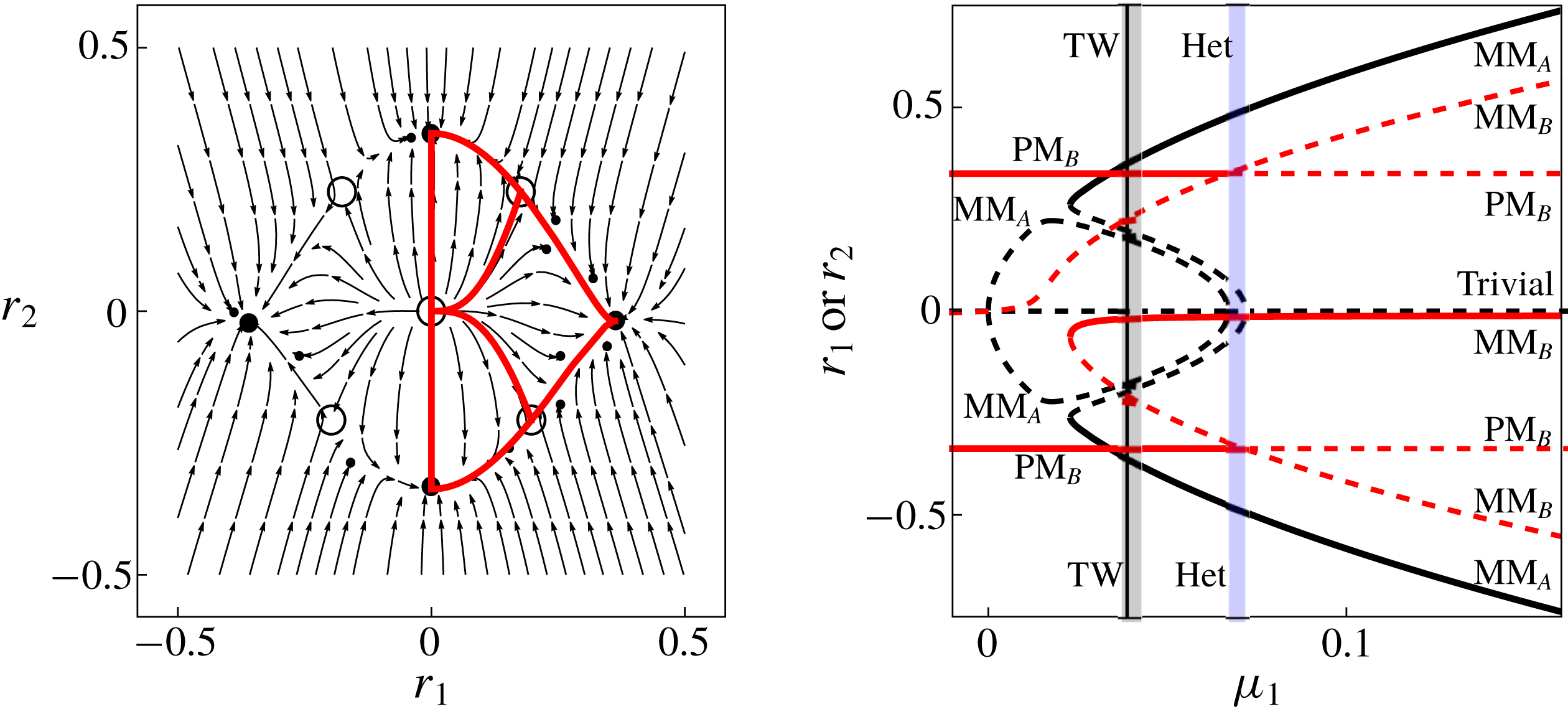
(i) Trivial solutions that arise when
 $\unicode[STIX]{x1D719}=r_{1}=r_{2}=0$
. They are stable when both
 $\unicode[STIX]{x1D707}_{1}$
and
 $\unicode[STIX]{x1D707}_{2}$
are negative and are unstable otherwise.
(ii) Non-travelling steady-state pure mode (PM) solutions with
 $r_{1}=0$
,
 $r_{2}=\pm \sqrt{-\unicode[STIX]{x1D707}_{2}/e_{22}}$
and
 $\unicode[STIX]{x1D719}=m\unicode[STIX]{x03C0}$
, where
 $m$
is integer. The PM bifurcates from the trivial solution when
 $\unicode[STIX]{x1D707}_{2}$
trespasses through zero and its stability can be determined from the signs of the eigenvalues. The scenario
 $r_{1}\neq 0$
and
 $r_{2}=0$
is not realisable.
(iii) Non-travelling mixed mode (MM) equilibrium solutions. These differ from PM solutions because both
 $r_{1}$
and
 $r_{2}$
are non-zero. The MM solutions bifurcate from trivial solutions when the PM solution is destabilised; MM solutions can also bifurcate from the trivial solution.
(iv) Travelling wave (TW) solutions resulting from equilibria with
 $\unicode[STIX]{x1D719}\neq m\unicode[STIX]{x03C0}$
.
Further classes of solutions that were identified by Armbruster et al. (Reference Armbruster, Guckenheimer and Holmes1988) and are not evident in this study include: standing wave solutions that arise when an MM solution undergoes a Hopf bifurcation; modulated travelling waves resulting from a TW solution undergoing a Hopf bifurcation; and heteroclinic cycles (Het) arising from trajectories connecting two PM solutions.
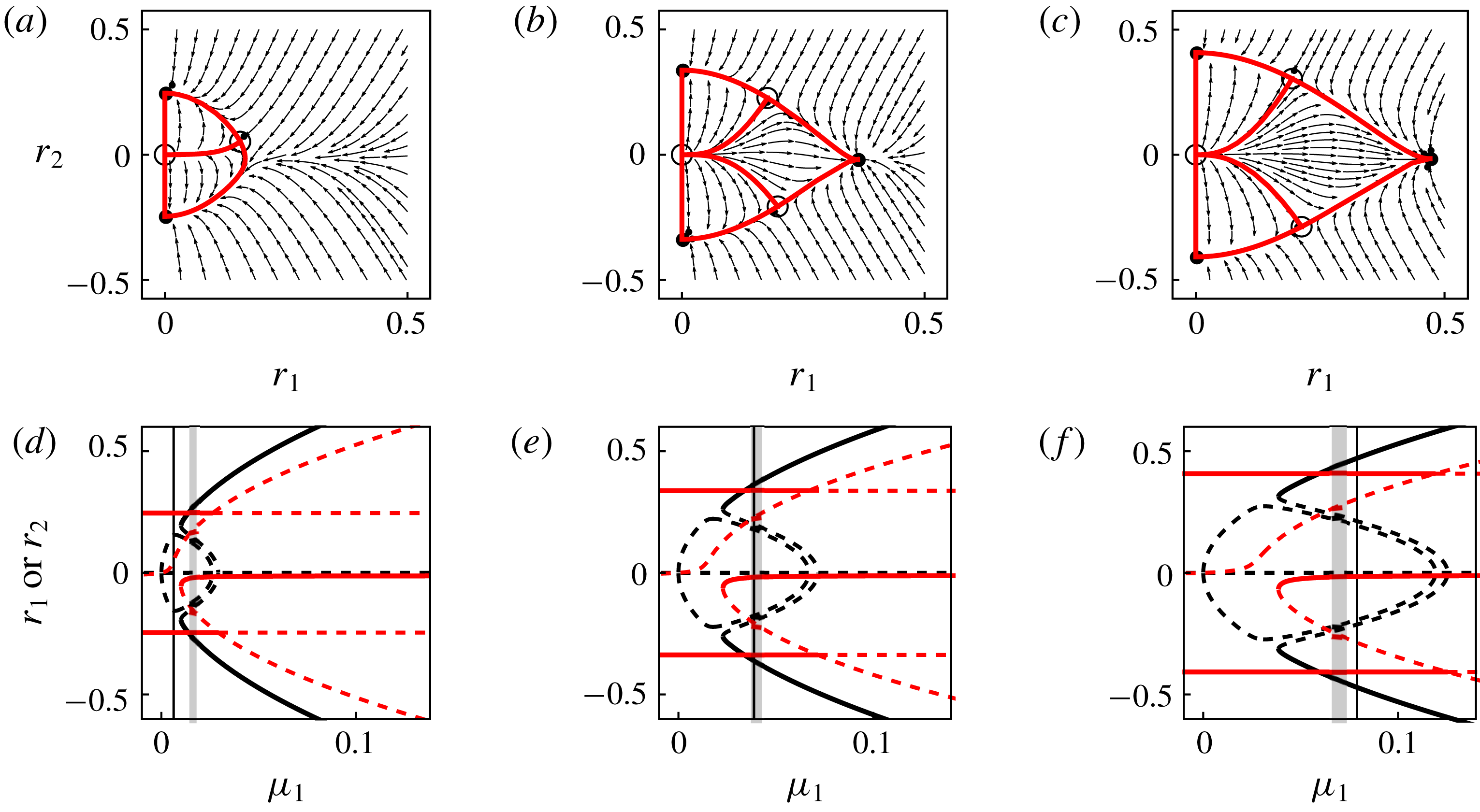
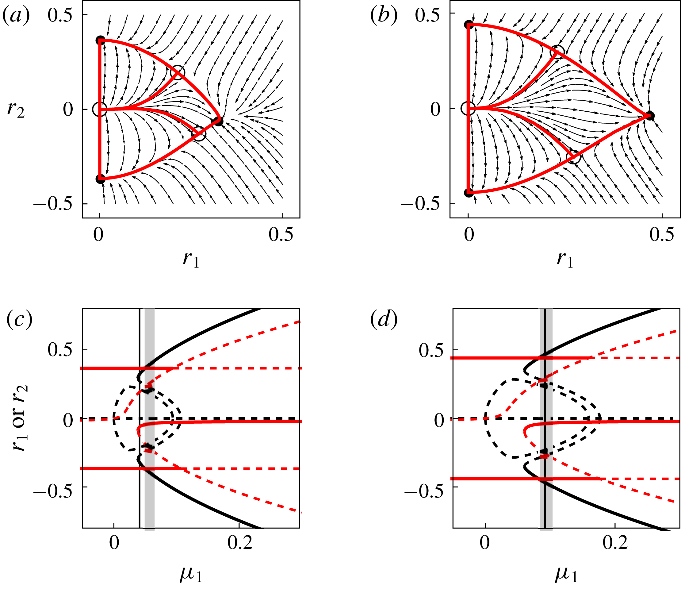
Phase plot and bifurcation diagram of (5.6) for 1 : 2 resonance with
 $\unicode[STIX]{x1D6FE}=0.03$
at
 ${\mathcal{R}}=1.2{\mathcal{R}}_{c}$
.


5.2 A 1 : 2 resonance example when
$\unicode[STIX]{x1D6FE}=0.03$

Consider now an example in which
 $\unicode[STIX]{x1D6FE}=0.03$
and
 ${\mathcal{R}}=1.2{\mathcal{R}}_{c}$
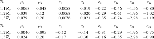
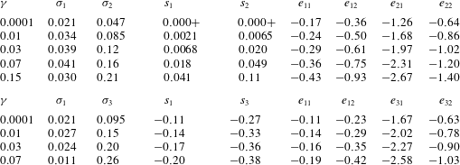
. Then on employing coefficients from table 3, (5.2) becomes
 $$\begin{eqnarray}\displaystyle & \displaystyle \dot{{\mathcal{A}}}=\unicode[STIX]{x1D707}_{1}{\mathcal{A}}+0.0068\overline{{\mathcal{A}}}{\mathcal{B}}-0.29{\mathcal{A}}|{\mathcal{A}}|^{2}-0.61{\mathcal{A}}|{\mathcal{B}}|^{2}, & \displaystyle\end{eqnarray}$$
 $$\begin{eqnarray}\displaystyle & \displaystyle \dot{{\mathcal{B}}}=\unicode[STIX]{x1D707}_{2}{\mathcal{B}}-0.02{\mathcal{A}}^{2}-1.96{\mathcal{B}}|{\mathcal{A}}|^{2}-1.02{\mathcal{B}}|{\mathcal{B}}|^{2}, & \displaystyle\end{eqnarray}$$
 $$\begin{eqnarray}\displaystyle & \displaystyle {\dot{r}}_{1}=\unicode[STIX]{x1D707}_{1}r_{1}+0.0068r_{1}r_{2}\cos \unicode[STIX]{x1D719}-0.29r_{1}^{3}-0.61r_{1}r_{2}^{2}, & \displaystyle\end{eqnarray}$$
 $$\begin{eqnarray}\displaystyle & \displaystyle {\dot{r}}_{2}=\unicode[STIX]{x1D707}_{2}r_{2}-0.02r_{1}^{2}\cos \unicode[STIX]{x1D719}-1.96r_{2}r_{1}^{2}-1.02r_{2}^{3}, & \displaystyle\end{eqnarray}$$
 $$\begin{eqnarray}\displaystyle & \displaystyle \dot{\unicode[STIX]{x1D719}}=\left(0.02\frac{r_{1}^{2}}{r_{2}}-0.014r_{2}\right)\sin \unicode[STIX]{x1D719} & \displaystyle\end{eqnarray}$$
 $\unicode[STIX]{x1D707}_{1}$
and
 $\unicode[STIX]{x1D707}_{2}$
have the values
 $$\begin{eqnarray}\displaystyle \unicode[STIX]{x1D707}_{1}=\unicode[STIX]{x1D70E}_{1}=0.039\quad \text{and}\quad \unicode[STIX]{x1D707}_{2}=\unicode[STIX]{x1D70E}_{2}=0.12. & & \displaystyle\end{eqnarray}$$
5.2.1 Phase plot
A phase plot of (5.6) with the parameter values (5.7) is shown in figure 5. For clarity it shows only flow in the
 $(r_{1},r_{2})$
plane and depicts streamlines of the vector field, together with separatrices (red), attractors (dots) and repellors (circles). Each attractor has its own basin of attraction and the basin boundaries are partially marked by the red separatrices. There are four attractors: two PM solutions that lie on the
 $r_{1}$
axis and two MM solutions just below the
 $r_{2}$
axis that result from the 1 : 2 resonance terms. The phase plot thus has left–right symmetry (i.e. it is invariant under
 $r_{1}\rightarrow -r_{1}$
), but up-down (
 $r_{2}\rightarrow -r_{2}$
) symmetry is broken slightly by stable MM solutions.
Note that (5.6) with parameters (5.7) is bistable, in the sense that, depending on initial conditions, the solution can be either a PM or an MM. Moreover, PM solutions arise when
 $r_{1}=0$
and
 $r_{2}\neq 0$
, which means that the only non-zero mode is the fundamental mode
 ${\mathcal{B}}$
of wavenumber
 $2l$
, in accord with linear theory. In this instance an observed surface field of windrows would remain almost stationary, parallel and spanwise periodic, much as in the Rodeo Lagoon photographs of Szeri (Reference Szeri1996).
In contrast MM solutions arise when
 $r_{1}\neq 0$
and
 $r_{2}\neq 0$
with
 $r_{1}\gg r_{2}$
, which means that a smaller-amplitude
 ${\mathcal{B}}$
-mode coexists with a dominant larger-amplitude
 ${\mathcal{A}}$
-mode. Since modes
 ${\mathcal{A}}$
and
 ${\mathcal{B}}$
have respective wavenumbers
 $l$
and
 $2l$
, it further means that MM solutions are likely to manifest as well-defined subharmonic cells (large-spaced) accompanied by weaker smaller-spaced fundamental modes. These would appear as stronger, weaker, stronger windrows.
Of course, in some instances, 1 : 2 resonance also allows for solutions that transit from PM to MM solutions or vice versa. For example a PM at (
 $r_{1},0$
) within the MM basin of attraction would transit to an MM at (
 $r_{1},r_{2}$
). Conversely, an MM solution at any
 $(r_{1},r_{2})$
within the PM basin of attraction would transit to a PM. This process would lead to windrows that meander and in some instances form Y-junctions. Both occurrences are widely observed, although Y-junctions occur sporadically and are not an equilibrium solution.
Finally, returning now to figure 1, we see that the subharmonic at
 ${\mathcal{R}}=1.2{\mathcal{R}}_{c}$
lies outside the Eckhaus-stability boundary rendering it nonlinearly unstable while the fundamental is within the boundary and nonlinearly stable. Nevertheless the two modes are susceptible to 1 : 2 resonance for some initial conditions and can double the LC spacing and halve the aspect ratio. This occurrence highlights the inadequacy of Eckhaus instability analysis to explain pattern selection in LC.
5.2.2 Bifurcation diagram
To gain further insight into the bistability evidenced in the phase plot, and also to determine over what parameter range it occurs, we defer to the bifurcation diagram of (5.6) in figure 5. Therein we fix
 $\unicode[STIX]{x1D707}_{2}$
at
 $\unicode[STIX]{x1D70E}_{2}$
and vary
 $\unicode[STIX]{x1D707}_{1}$
. Of course we could instead vary both
 $\unicode[STIX]{x1D707}_{1}$
and
 $\unicode[STIX]{x1D707}_{2}$
, as would occur with a change in the control parameter
 ${\mathcal{R}}$
; but doing so turns the problem into a codimension-2 bifurcation problem that provides no additional insight into our understanding of the phase plot (Porter & Knobloch Reference Porter and Knobloch2001). Instead we hold
 ${\mathcal{R}}$
constant, which fixes the least stable growth rate
 $\unicode[STIX]{x1D707}_{2}$
, and vary
 $\unicode[STIX]{x1D707}_{1}$
by slightly altering the wavenumber from that of the subharmonic, in essence by detuning the resonance.
Equilibrium amplitudes of
 $r_{1}$
are black in the bifurcation diagram, while those for
 $r_{2}$
are red. Moreover solid curves represent stable solutions and dashed curves unstable ones. There are also two coloured vertical bands. The blue band marks the range in which heteroclinic orbits may occur, although herein they are obstructed by stable MM solutions that are large in
 $|r_{1}|$
(Armbruster et al.
Reference Armbruster, Guckenheimer and Holmes1988). Because of that, heteroclinic regions are excluded in all subsequent cases. The second band is grey and defines the region in which TW solutions exist; however, they are never realised by the system because they are always unstable.
Inside the grey band is a black line that marks the position of
 $\unicode[STIX]{x1D70E}_{1}$
on the
 $\unicode[STIX]{x1D707}_{1}$
axis. Of note is that this line falls within the range in which both PM and MM solutions are stable, thereby confirming bistability. Furthermore, since the bifurcation diagram shows that the parameter range for bistability to occur is reasonably wide, we infer that bistability is robust, i.e. not sensitive to small variations in
 $\unicode[STIX]{x1D707}_{1}$
, as would occur from fluctuations in
 ${\mathcal{R}}$
. Finally, similar conclusions result if we fix
 $\unicode[STIX]{x1D707}_{1}$
and vary
 $\unicode[STIX]{x1D707}_{2}$
, but we will not present the details.
6 Langmuir circulation in 1 : 3 resonance
We turn now to 1 : 3 resonances between the least stable linear mode and its subharmonic, as indicated in figures 1 and 2. Of course studies of 1 : 3 resonance have a long history (Dangelmayr Reference Dangelmayr1986; Mizushima & Fujimura Reference Mizushima and Fujimura1992; Porter & Knobloch Reference Porter and Knobloch2000), but not in LC. Of note is that the amplitude equations (6.2) differ from their 1 : 2 counterparts (5.2) in that they contain no quadratic terms.
6.1 Amplitude equations for 1 : 3 resonance
Consonant with our derivation in § 5.1, we here set
 $3l$
to be the wavenumber of the fundamental and its subharmonic be
 $l$
. We then assume that in the weakly nonlinear regime (Mizushima & Fujimura Reference Mizushima and Fujimura1992)
 $$\begin{eqnarray}\displaystyle \left(\begin{array}{@{}c@{}}u\\ \unicode[STIX]{x1D713}\end{array}\right)=\left(\begin{array}{@{}c@{}}A(T)u_{A}(z)\text{e}^{\text{i}ly}+C(T)u_{C}(z)\text{e}^{3\text{i}ly}\\ A(T)\unicode[STIX]{x1D713}_{A}(z)\text{e}^{\text{i}ly}+C(T)\unicode[STIX]{x1D713}_{C}(z)\text{e}^{3\text{i}ly}\end{array}\right)+\text{c.c.} & & \displaystyle\end{eqnarray}$$
in which
 $A(T)$
and
 $C(T)$
are unknown slowly varying amplitudes, and
 $(u,\unicode[STIX]{x1D713})_{A}$
and
 $(u,\unicode[STIX]{x1D713})_{C}$
are eigenfunctions for the respective subharmonic and the fundamental.
Then, by entirely similar procedures to those in § 5.1, the amplitude equations governing
 $A(T)$
and
 $C(T)$
follow as
 $$\begin{eqnarray}\displaystyle & \displaystyle {\dot{A}}=\unicode[STIX]{x1D707}_{1}A+s_{1}\overline{A}^{2}C+e_{11}A|A|^{2}+e_{12}A|C|^{2}, & \displaystyle\end{eqnarray}$$
 $$\begin{eqnarray}\displaystyle & \displaystyle {\dot{C}}=\unicode[STIX]{x1D707}_{3}C+s_{3}A^{3}+e_{31}C|A|^{2}+e_{32}C|C|^{2} & \displaystyle\end{eqnarray}$$
 $\unicode[STIX]{x1D707}_{1}$
and
 $\unicode[STIX]{x1D707}_{3}$
are linear growth rates of the subharmonic and the fundamental at specified
 ${\mathcal{R}}>{\mathcal{R}}_{c}$
while the coefficients
 $e_{ij}$
and
 $s_{i}$
are real numbers.
Accordingly on setting
 $$\begin{eqnarray}\displaystyle A=r_{1}\text{e}^{\text{i}\unicode[STIX]{x1D703}_{1}},\quad C=r_{3}\text{e}^{\text{i}\unicode[STIX]{x1D703}_{3}}\quad \text{and}\quad \unicode[STIX]{x1D719}=-3\unicode[STIX]{x1D703}_{1}+\unicode[STIX]{x1D703}_{3}, & & \displaystyle\end{eqnarray}$$
(6.2) can be transformed to polar form as
 $$\begin{eqnarray}\displaystyle & \displaystyle {\dot{r}}_{1}=\unicode[STIX]{x1D707}_{1}r_{1}+s_{1}r_{1}^{2}r_{3}\cos \unicode[STIX]{x1D719}+e_{11}r_{1}^{3}+e_{12}r_{1}r_{3}^{2}, & \displaystyle\end{eqnarray}$$
 $$\begin{eqnarray}\displaystyle & \displaystyle {\dot{r}}_{3}=\unicode[STIX]{x1D707}_{3}r_{3}+s_{3}r_{1}^{3}\cos \unicode[STIX]{x1D719}+e_{31}r_{3}r_{1}^{2}+e_{32}r_{3}^{3} & \displaystyle\end{eqnarray}$$
and
 $$\begin{eqnarray}\displaystyle \dot{\unicode[STIX]{x1D719}}=\left(-s_{3}\frac{r_{1}^{3}}{r_{3}}-3s_{1}r_{1}r_{3}\right)\sin \unicode[STIX]{x1D719}. & & \displaystyle\end{eqnarray}$$
6.2 Solutions to the 1 : 3 resonance equation
In considering possible solutions to (6.4) we look first for TW solutions defined by (6.4c
). In particular we seek solutions for
 $\dot{\unicode[STIX]{x1D719}}=0$
at arbitrary
 $r_{1}$
and
 $r_{3}$
, which requires either the bracketed term or
 $\sin \unicode[STIX]{x1D719}$
in (6.4c
) be zero. The bracketed term relates the amplitudes
 $r_{1}$
and
 $r_{3}$
through
 $$\begin{eqnarray}\displaystyle r_{1}=\pm r_{3}\sqrt{-\frac{3s_{1}}{s_{3}}}. & & \displaystyle\end{eqnarray}$$
But because
 $r_{1}$
and
 $r_{3}$
are strictly real,
 $s_{1}s_{3}$
must be negative for (6.5) to be meaningful, whereas in our study
 $s_{1}s_{3}$
is positive. Solutions for
 $\dot{\unicode[STIX]{x1D719}}=0$
are therefore possible only if
 $\unicode[STIX]{x1D719}=0$
or
 $\unicode[STIX]{x1D719}=\pm \unicode[STIX]{x03C0}$
etc., giving rise to standing (non-travelling) waves. Thus, in the absence of a tangible case for TW and modulated TW solutions (Porter & Knobloch Reference Porter and Knobloch2000) we instead satisfy
 $\dot{\unicode[STIX]{x1D719}}=0$
by setting
 $\unicode[STIX]{x1D719}=0$
, which decouples (6.4c
) from (6.4a
), (6.4b
).
Decoupling (6.4c ) further means that we can ignore it and concentrate on solutions to the remaining equations
 $$\begin{eqnarray}\displaystyle {\dot{r}}_{1}=\unicode[STIX]{x1D707}_{1}r_{1}+s_{1}r_{1}^{2}r_{3}+e_{11}r_{1}^{3}+e_{12}r_{1}r_{3}^{2}, & & \displaystyle\end{eqnarray}$$
and
 $$\begin{eqnarray}\displaystyle {\dot{r}}_{3}=\unicode[STIX]{x1D707}_{3}r_{3}+s_{3}r_{1}^{3}+e_{31}r_{3}r_{1}^{2}+e_{32}r_{3}^{3}. & & \displaystyle\end{eqnarray}$$
First, we note that (6.6) has the trivial solution
 $r_{1}=r_{3}=0$
with eigenvalues
 $\unicode[STIX]{x1D707}_{1}$
and
 $\unicode[STIX]{x1D707}_{3}$
. Second, we see that PM solutions are possible when
 $r_{1}=0$
and
 $r_{3}=\pm \sqrt{-\unicode[STIX]{x1D707}_{3}/e_{32}}$
and that MM solutions are also possible, although their expressions are lengthy so we exclude them. We do, however, note that while in principle there can also be standing waves and heteroclinic orbits (Porter & Knobloch Reference Porter and Knobloch2000), we found neither. Finally, (6.6) is equivariant under the reflection or inversion
 $r_{1}\rightarrow -r_{1}$
and
 $r_{3}\rightarrow -r_{3}$
.
6.3 A 1 : 3 resonance example when
$\unicode[STIX]{x1D6FE}=0.03$

Consider now an example in which
 $\unicode[STIX]{x1D6FE}=0.03$
and
 ${\mathcal{R}}=1.3{\mathcal{R}}_{c}$
, as shown in figure 1. Then from table 3, (6.6) reads
 $$\begin{eqnarray}\displaystyle & \displaystyle {\dot{r}}_{1}=\unicode[STIX]{x1D707}_{1}r_{1}-0.17r_{1}^{2}r_{3}-0.16r_{1}^{3}-0.35r_{1}r_{3}^{2}, & \displaystyle\end{eqnarray}$$
 $$\begin{eqnarray}\displaystyle & \displaystyle {\dot{r}}_{3}=\unicode[STIX]{x1D707}_{3}r_{3}-0.36r_{1}^{3}-2.28r_{3}r_{1}^{2}-0.90r_{3}^{3} & \displaystyle\end{eqnarray}$$
 $$\begin{eqnarray}\displaystyle \unicode[STIX]{x1D707}_{1}=\unicode[STIX]{x1D70E}_{1}=0.024\quad \text{and}\quad \unicode[STIX]{x1D707}_{3}=\unicode[STIX]{x1D70E}_{3}=0.20. & & \displaystyle\end{eqnarray}$$
The phase plot and bifurcation diagram for (6.7) with coefficients (6.8) are given in figure 6, whose schema is the same as figure in 5, albeit with
 $r_{2}$
replaced by
 $r_{3}$
. Looking first to the phase plot we immediately see the
 $(r_{1},r_{3})\rightarrow (-r_{1},-r_{3})$
symmetry anticipated above, in which one stable MM solution is located in the second quadrant, while its counterpart is located in the fourth quadrant. Stable MM solutions again arise with
 $|r_{1}|$
larger than
 $|r_{3}|$
, but rather than being disparate as in our example in § 5.2, their magnitudes here are of the same order, suggesting that the two modes would generate windrows of comparable strength and have the same observability.
Bistability also occurs, although the basins of attraction of the MM solutions are relatively small compared with those of the PM solutions. The reason why is evident in the bifurcation diagram, in which we see that the line marking the position of
 $\unicode[STIX]{x1D70E}_{1}$
is almost at the leftmost boundary of the bistability range. In fact stable MM solutions would vanish if
 $\unicode[STIX]{x1D707}_{1}$
were further reduced and the only attractors would be PM solutions. Finally, although their basin of attraction is small for the limited range of
 ${\mathcal{R}}$
we have investigated, the existence of MM solutions again highlights that resonance can, for some initial conditions, substantially modify the dynamics suggested by the Eckhaus boundary.
Phase plot and bifurcation diagram of (6.7) for 1 : 3 resonance with
 $\unicode[STIX]{x1D6FE}=0.03$
at
 ${\mathcal{R}}=1.3{\mathcal{R}}_{c}$
.

7 The roles of
${\mathcal{R}}$
and
$\unicode[STIX]{x1D6FE}$
on resonance


Up to this point we have focused on 1 : 2 and 1 : 3 resonance at fixed
 ${\mathcal{R}}$
and fixed
 $\unicode[STIX]{x1D6FE}$
. Our intent now is to consider a range of
 ${\mathcal{R}}$
and
 $\unicode[STIX]{x1D6FE}$
to determine how they affect the dynamics. To that end we first hold
 $\unicode[STIX]{x1D6FE}$
constant and vary
 ${\mathcal{R}}$
.
7.1 The role of
${\mathcal{R}}$
at constant
$\unicode[STIX]{x1D6FE}$


Specifically, we set
 $\unicode[STIX]{x1D6FE}=0.03$
as before and consider
 ${\mathcal{R}}=1.1{\mathcal{R}}_{c},1.2{\mathcal{R}}_{c}$
and
 $1.3{\mathcal{R}}_{c}$
; the coefficients required in the amplitude equations (5.2) and (6.2) are listed in table 3. Phase portraits (displaying only the first and fourth quadrants because of symmetry) and bifurcation diagrams are shown in figures 7 and 8.
Looking first at the phase portraits for 1 : 2 resonance (figure 7), we see at
 $1.1{\mathcal{R}}_{c}$
that only PM solutions are stable, while both stable PM and stable MM solutions are present at
 $1.2{\mathcal{R}}_{c}$
, indicating that onset to bistability occurs at an
 ${\mathcal{R}}$
somewhere in between. Moreover as
 ${\mathcal{R}}$
increases further, the relative area of the basins of attraction of the stable MM solutions and their amplitudes grow, as do the amplitudes of the PM solutions.
This scenario highlights a substantial departure from linear instability theory where, as seen by the coefficients in table 3, the growth rate
 $\unicode[STIX]{x1D70E}_{2}=\unicode[STIX]{x1D707}_{2}$
of the fundamental mode always exceeds that of the subharmonic. Indeed, even though the ratio
 $\unicode[STIX]{x1D70E}_{1}/\unicode[STIX]{x1D70E}_{2}$
increases with
 ${\mathcal{R}}$
, it only reaches approximately 0.4 at
 ${\mathcal{R}}=1.3{\mathcal{R}}_{c}$
, suggesting that the fundamental dominates. In contrast, 1 : 2 resonance can lead to the obverse.
Turning now to 1 : 3 resonance, we note that since the subharmonic for
 $1.1{\mathcal{R}}_{c}$
lies outside the neutral curve we exclude it and present in figure 8 only the two higher
 ${\mathcal{R}}$
s. Of particular interest as
 ${\mathcal{R}}$
increases from
 $1.2{\mathcal{R}}_{c}$
to
 $1.3{\mathcal{R}}_{c}$
, is that the ratio
 $\unicode[STIX]{x1D70E}_{1}/\unicode[STIX]{x1D70E}_{3}$
grows from approximately
 $0.05$
to
 $0.12$
, causing
 $\unicode[STIX]{x1D707}_{1}$
to move into the bistability region, ensuring stable MM solutions.
Phase plots and bifurcation diagrams for 1 : 2 resonance at
 ${\mathcal{R}}=1.1{\mathcal{R}}_{c}$
(a,d),
 ${\mathcal{R}}=1.2{\mathcal{R}}_{c}$
(b,e) and
 ${\mathcal{R}}=1.3{\mathcal{R}}_{c}$
(c,f) with
 $\unicode[STIX]{x1D6FE}=0.03$
.


Phase plots and bifurcation diagrams for 1 : 3 resonance at
 ${\mathcal{R}}=1.2{\mathcal{R}}_{c}$
(a,c) and
 ${\mathcal{R}}=1.3{\mathcal{R}}_{c}$
(b,d) with
 $\unicode[STIX]{x1D6FE}=0.03$
. The
 ${\mathcal{R}}=1.1{\mathcal{R}}_{c}$
case is absent because the subharmonic lies outside the neutral curve.

7.2 The role of
$\unicode[STIX]{x1D6FE}$
on 1 : 2 resonance

In considering the role of
 $\unicode[STIX]{x1D6FE}$
on 1 : 2 resonance, we first recall that the boundary conditions are symmetric when
 $\unicode[STIX]{x1D6FE}=0$
and gradually lose symmetry as
 $\unicode[STIX]{x1D6FE}$
increases. We further see from table 4 that
 $|s_{1}|$
and
 $|s_{2}|$
likewise increase with
 $\unicode[STIX]{x1D6FE}$
, suggesting that resonance strengthens as symmetry in the boundary conditions is gradually lost. Our focus in discussing the role of
 $\unicode[STIX]{x1D6FE}$
therefore is on the breaking of top–bottom symmetry. To that end we employ three values of
 $\unicode[STIX]{x1D6FE}$
ranging from
 $10^{-4}$
to
 $0.15$
, at three values of
 ${\mathcal{R}}$
, viz.
 ${\mathcal{R}}=1.1{\mathcal{R}}_{c},1.2{\mathcal{R}}_{c}$
and
 $1.3{\mathcal{R}}_{c}$
. Phase portraits and the bifurcation diagrams are displayed in figures 9 through to 11.
First, we see from table 4 at
 $\unicode[STIX]{x1D6FE}=10^{-4}$
that
 $|s_{1}|$
and
 $|s_{2}|$
are less than
 $10^{-4}$
, indicating that symmetry-breaking and thus resonance are essentially absent, a finding likewise reflected in the phase portraits and the bifurcation diagrams shown in figure 9. Because of that, bistability is seen to arise in the phase portraits through the co-existence of a PM solution on the
 $r_{2}$
axis and what approximates a PM solution on the
 $r_{1}$
axis, thereby excluding MM solutions below the
 $r_{2}$
axis.
Once
 $\unicode[STIX]{x1D6FE}$
is larger than 0.01, however, the values
 $s_{1}$
and
 $s_{2}$
are no longer negligible and asymmetries are evident, particularly in the phase plots of figure 7, where
 $\unicode[STIX]{x1D6FE}=0.03$
. Specifically, one of the PM solutions at
 $(r_{1},0)$
is replaced by a stable MM solution with large
 $r_{1}$
and small
 $r_{2}$
in the fourth quadrant. Asymmetry is also reflected in the bifurcation diagrams where, what is a pitchfork bifurcation in figure 9, becomes an imperfect pitchfork in figure 7. Unstable TW solutions are also possible.
The effects of symmetry breaking become more significant as
 $\unicode[STIX]{x1D6FE}$
increases further to 0.07, as seen in figure 10. Specifically, the band in which TW solutions exist widens, and the value of
 $r_{2}$
defining MM solutions become larger. The MM solutions also become more difficult to realise in the range of
 ${\mathcal{R}}$
considered, because their basins of attraction are eroded by the expanding attraction basins for PM solutions. The reason for this PM encroachment can be seen in the bifurcation diagram, in which the vertical line marking the value of
 $\unicode[STIX]{x1D70E}_{1}$
moves just to the left of the bistable range.
Indeed, as we see in figure 11 for
 $\unicode[STIX]{x1D6FE}=0.15$
, the PM basins can swamp the whole phase plane, even when
 ${\mathcal{R}}=1.3{\mathcal{R}}_{c}$
and fall into a range in which only PM solutions are admitted. Of course this does not exclude bistability at larger
 $R$
, where the subharmonics will move further inside the neutral curve, because the parameter range over which bistability occurs is wide, suggesting that it is also robust.
Phase plots and bifurcation diagrams for 1 : 2 resonance at
 ${\mathcal{R}}=1.1{\mathcal{R}}_{c}$
(a,d),
 ${\mathcal{R}}=1.2{\mathcal{R}}_{c}$
(b,e) and
 ${\mathcal{R}}=1.3{\mathcal{R}}_{c}$
(c,f) with
 $\unicode[STIX]{x1D6FE}=10^{-4}$
.

Phase plots and bifurcation diagrams for 1 : 2 resonance at
 ${\mathcal{R}}=1.2{\mathcal{R}}_{c}$
(a,c) and
 ${\mathcal{R}}=1.3{\mathcal{R}}_{c}$
(b,d) with
 $\unicode[STIX]{x1D6FE}=0.07$
. The
 ${\mathcal{R}}=1.1{\mathcal{R}}_{c}$
case is absent because the subharmonic lies outside the neutral curve.

Phase plots and bifurcation diagrams for 1 : 2 resonance at
 ${\mathcal{R}}=1.3{\mathcal{R}}_{c}$
with
 $\unicode[STIX]{x1D6FE}=0.15$
.

Phase plots and bifurcation diagrams for 1 : 3 resonance at
 ${\mathcal{R}}=1.1{\mathcal{R}}_{c}$
(a,d),
 ${\mathcal{R}}=1.2{\mathcal{R}}_{c}$
(b,e) and
 ${\mathcal{R}}=1.3{\mathcal{R}}_{c}$
(c,f) with
 $\unicode[STIX]{x1D6FE}=10^{-4}$
.

7.3 The role of
$\unicode[STIX]{x1D6FE}$
on 1 : 3 resonance

Turning now to the role of
 $\unicode[STIX]{x1D6FE}$
in 1 : 3 resonance and looking first to figure 1, we find that although the sub-harmonic lies within the neutral curve for all
 $R\geqslant 1.1R_{c}$
when
 $\unicode[STIX]{x1D6FE}=10^{-4}$
, that is so only at
 $R=1.3R_{c}$
when
 $\unicode[STIX]{x1D6FE}=0.07$
, thereby restricting our upper bound on
 $\unicode[STIX]{x1D6FE}$
. We further note that in contrast to 1 : 2 resonance, 1 : 3 resonance is unaffected by top–bottom symmetry (Prat, Mercader & Knobloch Reference Prat, Mercader and Knobloch1998). This is particularly evident from the values of
 $s_{1}$
and
 $s_{3}$
in table 4, which in contrast to their 1 : 2 resonance counterparts, barely double over the range of
 $\unicode[STIX]{x1D6FE}$
.
Looking first to figure 12 (at
 $\unicode[STIX]{x1D6FE}=10^{-4}$
) we again find robust bistability and reasonably large basins of attraction for PM solutions, but the basins attracting MM solutions rapidly shrink or even vanish as
 $\unicode[STIX]{x1D6FE}$
increases, as we see at
 $\unicode[STIX]{x1D6FE}=0.03$
(figure 8) and
 $\unicode[STIX]{x1D6FE}=0.07$
(figure 13). That said, the basins of attraction for MM solutions may not necessarily be small at higher
 ${\mathcal{R}}$
, because the subharmonic can lie further inside the neutral curve, thereby increasing their chance of survival.
Phase plots and bifurcation diagrams for 1 : 3 resonance at
 ${\mathcal{R}}=1.3{\mathcal{R}}_{c}$
with
 $\unicode[STIX]{x1D6FE}=0.07$
.

8 Conclusion
Foam and other tracers that are swept into the surface convergence zones of LC highlight not only their footprints but recurrent, sporadic, Y-junctions. These junctions characterise not only a half spacing translation but also, and more commonly, a change in spacing, be it from narrow to wide, wide to narrow or both. Of key interest herein are what nonlinear mechanisms trigger that change.
We proceed by assuming the initial spacing is set by linear instability theory and that changes in spacing result from nonlinearities. To that end we employ the prevailing theory for LC, the mean field CL equations of Craik & Leibovich (Reference Craik and Leibovich1976), and solve them in a construct devised by Cox & Leibovich (Reference Cox and Leibovich1993) that captures events both in a layer above deeper water separated by a thermocline and a layer bounded by a slippery rigid bottom. We further assume that LC form via the CL2 instability and that the wave-mean flow underlying it is characterised by uniform shear and differential drift, to wit
 $U^{\prime }=D^{\prime }=1$
. In the absence of stratification, only two parameters remain in our study: a Rayleigh number
 ${\mathcal{R}}$
in the CL equations and what amounts to a symmetry breaking parameter
 $\unicode[STIX]{x1D6FE}$
, in the free surface boundary conditions.
Looking first to linear instability theory over the range
 $\unicode[STIX]{x1D6FE}\in (0,1]$
suggested by Phillips & Dai (Reference Phillips and Dai2014), we find in figure 2 that the neutral curves near onset evolve from asymmetric as
 $\unicode[STIX]{x1D6FE}\rightarrow 0$
, to almost symmetric as
 $\unicode[STIX]{x1D6FE}\rightarrow 1$
. Evident too as
 $\unicode[STIX]{x1D6FE}$
increases, is that
 $({\mathcal{R}}_{c},l_{c})$
pairs increase from the lower bound
 $(120,0)$
at
 $\unicode[STIX]{x1D6FE}=0$
(Cox & Leibovich Reference Cox and Leibovich1993). Put differently, the spacing of columnar LC pairs at onset decreases as
 $\unicode[STIX]{x1D6FE}$
increases. Finally, as expected, no jumps in spacing were observed since the Prandtl number is constant (Phillips Reference Phillips2001).
Spacing changes can, of course, result from nonlinearities and to investigate such effects we turn to weakly nonlinear theory and begin by deriving an amplitude equation of Ginzburg–Landau type that allows us to explore the nonlinear dynamics of single modes, i.e. modes excited nonlinearly that do not interact. This approach has not previously been utilised in the context of LC and we find that although the Ginzburg–Landau equation is usually of cubic order when the bifurcation is supercritical, as it is here, we must proceed to quartic order to capture that asymmetric behaviour of the neutral curves. This equation is then subjected to an Eckhaus instability analysis, from which we determine Eckhaus stability boundaries. As seen in figures 1 and 2, these boundaries lie within the neutral curves, but of key interest in determining surface patterns, is whether the linearly least stable wavenumbers and their harmonics lie within the Eckhaus boundaries. Interestingly, although the least stable wavenumbers for most
 $\unicode[STIX]{x1D6FE}$
do live inside, their subharmonics do not, which means that they are not candidates for nonlinear excitation and that the surface pattern is unchanged from its linear counterpart.
However, that is not the complete story, because as
 $\unicode[STIX]{x1D6FE}$
diminishes toward zero, the least stable mode moves outside the Eckhaus boundary and the subharmonics inside. This excludes the fundamental and means instead that the subharmonics, or indeed any wavenumber within the Eckhaus boundary, are candidates for excitation, necessitating an increase in spacing. This concurs with the findings of Hayes & Phillips (Reference Hayes and Phillips2017), who considered nonlinear equilibrium states in the small spanwise-wavenumber limit (with
 $\unicode[STIX]{x1D6FE}\ll 1$
) in the absence of mode interactions, and find that the spacing increase is precipitated by a break in up-down symmetry. However, there is no mechanism by which spacing can increase beyond that determined by the Eckhaus boundary and thus no further Y-junctions. Because of that we conclude that the nonlinear excitation of single modes is not a candidate to explain Farmer & Li’s (Reference Farmer and Li1995) observations of multiple Y-junctions and spacing changes, although the
 $\unicode[STIX]{x1D6FE}\ll 1$
scenario is reminiscent of the high aspect ratio LC observed beneath long waves in shallow water reported by Marmorino et al. (Reference Marmorino, Smith and Lindemann2005). To wit, another mechanism is necessarily at play, an obvious candidate being one centred on nonlinear interactions between the modes.
To that end we next explore 1 : 2 and 1 : 3 resonance based upon coupled amplitude equations of Stuart-Landau type for the least stable linear mode and its subharmonic. Herein we find that the equations for 1 : 2 resonance include quadratic terms, while the 1 : 3 equations do not, which renders the former susceptible to top–bottom symmetry and the latter not, although
 $\unicode[STIX]{x1D6FE}$
continues to play a role in both, albeit a far weaker role in 1 : 3.
Of the classes of solutions to Stuart-Landau equations identified by Armbruster et al. (Reference Armbruster, Guckenheimer and Holmes1988), the most prevalent here, both in 1 : 2 and 1 : 3 resonance, are non-travelling stable pure-mode solutions and non-travelling stable mixed-mode solutions that often coexist, to realise generically robust bistable solutions. Of particular interest is that these solutions can, for certain initial conditions, double or even triple the dominant spacing relative to that predicted by linear theory, even when the large-spaced modes lie outside the Eckhaus-stable boundary computed by the quartic-order Ginzburg–Landau equation. Bistability also provides an explanation for recurrent Y-junctions because, during a resonance event and depending on initial conditions, the dominant pattern can switch from wide to narrow, or narrow to wide, especially when a large-amplitude subharmonic mode is accompanied by a small-amplitude fundamental mode.
Furthermore, since ever more subharmonics live within the neutral curve as
 ${\mathcal{R}}$
increases, there is the possibility of a cascade in spacing, leading to the devolution of dominant LC into a discrete spectrum of LC, although just how far from the primary instability threshold bistability acts, is unclear. What is clear, however, is that discrete spectra are ubiquitous, not only far from the primary instability threshold, but in the presence of complicating features such as three-dimensional effects, stratification and strong nonlinearity, as evident in large eddy simulation and direct numerical simulation calculations (McWilliams et al.
Reference McWilliams, Sullivan and Moeng1997; Tsai et al.
Reference Tsai, Chen, Lu and Garbe2013, Reference Tsai, Chen and Lu2015).
Left and right spanwise (cross-wind) travelling waves are also observed and the band in which they occur can be wide, see e.g. figure 11, but we ignore them because they are unstable and never realised. In contrast, sinuous and vacillating streamwise (downwind) propagating travelling waves feature strongly in the dynamics of surface patterns of LC when periodic variations in
 $x$
are permitted, as Tandon & Leibovich (Reference Tandon and Leibovich1995) find in direct numerical simulations of the CL equations. Zhang et al. (Reference Zhang, Chini, Julien and Knobloch2015) further report steady- and unsteady-defect travelling waves, the latter giving rise to downwind-modulated 1 : 2 spatial resonance. Thus, although
 $x$
-dependence is known to have little effect on the linearly most unstable modes (Leibovich & Tandon Reference Leibovich and Tandon1993), its exclusion would appear to thwart an alternate path to resonance between LC.
Acknowledgements
Our thanks to S. Suslov and an anonymous referee for their interest and helpful comments. This work was supported in part by the National Science Foundation under grant no. NSF PHY17-48958. L.C. was supported by a Victorian International Research Scholarship from the State Government of Victoria, Australia and by Swinburne University of Technology.
Appendix A. Closure of the amplitude expansion method
Here we provide an outline of the amplitude expansion method used in §§ 5–6 and in particular the optimised closure scheme of Pham & Suslov (Reference Pham and Suslov2018) employed therein, whose aim is to obtain amplitude equations that are valid far from the critical point on the marginal stability curve. Since their scheme can be illustrated by deriving the third-order Stuart-Landau equation governing the evolution of an isolated mode of amplitude
 $A$
, we derive it rather than the resonance equations (5.2) and (6.2). To proceed we employ the ansatz (5.1), let
 $E^{n}=\text{e}^{\text{i}nly}$
and, for both
 $\unicode[STIX]{x1D713}$
and
 $u$
, assume the expansion (Watson Reference Watson1960; Herbert Reference Herbert1983)
 $$\begin{eqnarray}\displaystyle \unicode[STIX]{x1D713}=(\unicode[STIX]{x1D700}E^{1}\unicode[STIX]{x1D713}_{11}A+\unicode[STIX]{x1D700}^{2}E^{2}\unicode[STIX]{x1D713}_{22}A^{2}+\unicode[STIX]{x1D700}^{3}E^{1}\unicode[STIX]{x1D713}_{13}A|A|^{2})+\unicode[STIX]{x1D700}^{2}\unicode[STIX]{x1D713}_{02}|A|^{2}+\text{c.c.} & & \displaystyle\end{eqnarray}$$
Then, on substituting (A 1) into (2.2b,c
) and boundary conditions (2.4), and collecting terms of the same order in
 $\unicode[STIX]{x1D700}$
and harmonic
 $E^{n}$
, we find a hierarchy of linear problems best expressed in terms of the linear operators and functions
 $$\begin{eqnarray}\displaystyle \unicode[STIX]{x1D613}_{k}=\left[\begin{array}{@{}cc@{}}[\text{N}-(kl)^{2}]^{2} & \text{i}{\mathcal{R}}(kl)D^{\prime }\\ \text{i}(kl)U^{\prime } & \text{N}-(kl)^{2}\end{array}\right],\quad \unicode[STIX]{x1D614}_{k}=\left[\begin{array}{@{}cc@{}}\text{N}-(kl)^{2} & 0\\ 0 & 1\end{array}\right], & & \displaystyle\end{eqnarray}$$
 $$\begin{eqnarray}\displaystyle \unicode[STIX]{x1D733}_{ij}=\left(\begin{array}{@{}c@{}}\unicode[STIX]{x1D713}_{ij}(z)\\ u_{ij}(z)\end{array}\right),\quad \boldsymbol{f}_{ij}(z)=\left(\begin{array}{@{}c@{}}f_{ij}(z)\\ g_{ij}(z)\end{array}\right) & & \displaystyle\end{eqnarray}$$
in which
 $i,j,k$
are integers. Moreover, as done in § 4.1, we further express time
 $t$
in terms of a fast scale
 $\hat{t}$
and slow scales
 $T_{m}=\unicode[STIX]{x1D700}^{m}t$
such that
 $\unicode[STIX]{x1D700}\unicode[STIX]{x2202}_{T}=\unicode[STIX]{x1D700}^{m}\unicode[STIX]{x2202}_{T_{m}}$
.
Since
 $A_{\hat{t}}=\unicode[STIX]{x1D70E}_{1}A$
at
 $O(\unicode[STIX]{x1D700})$
, we readily recover the linear eigenvalue problem
 $$\begin{eqnarray}\displaystyle (\unicode[STIX]{x1D70E}_{1}\unicode[STIX]{x1D614}_{1}-\unicode[STIX]{x1D613}_{1})\unicode[STIX]{x1D733}_{\mathbf{11}}=0, & & \displaystyle\end{eqnarray}$$
which can be solved numerically to realise the eigenfunctions
 $\unicode[STIX]{x1D733}_{\mathbf{11}}=(\unicode[STIX]{x1D713}_{11},u_{11})^{\text{T}}$
and eigenvalue
 $\unicode[STIX]{x1D70E}_{1}$
at any
 $R\geqslant {\mathcal{R}}_{c}$
. Similar linear problems, albeit inhomogeneous ones, arise at
 $O(\unicode[STIX]{x1D700}^{2})$
for
 $E^{0}$
,
 $E^{1}$
and
 $E^{2}$
from which, in addition to eigensolutions, we determine that
 $A_{T_{1}}=0$
.
Of particular interest, however, are details at
 $O(\unicode[STIX]{x1D700}^{3})$
, where by design only the
 $E^{1}$
harmonic is retained, yielding
 $$\begin{eqnarray}\displaystyle A|A|^{2}(\unicode[STIX]{x1D613}_{1}-3\unicode[STIX]{x1D70E}_{1}\unicode[STIX]{x1D614}_{1})\unicode[STIX]{x1D733}_{\mathbf{13}}=\frac{\unicode[STIX]{x2202}A}{\unicode[STIX]{x2202}T_{2}}\unicode[STIX]{x1D614}_{1}\unicode[STIX]{x1D733}_{\mathbf{11}}+A|A|^{2}\boldsymbol{f}_{13} & & \displaystyle\end{eqnarray}$$
in which
 $$\begin{eqnarray}\displaystyle f_{13}=\text{i}l(-6l^{2}\unicode[STIX]{x1D713}_{22}\overline{\unicode[STIX]{x1D713}}_{11}^{\prime }-3l^{2}\overline{\unicode[STIX]{x1D713}}_{11}\unicode[STIX]{x1D713}_{22}^{\prime }-\unicode[STIX]{x1D713}_{22}^{\prime }\overline{\unicode[STIX]{x1D713}}_{11}^{\prime \prime }+2\overline{\unicode[STIX]{x1D713}}_{11}^{\prime }\unicode[STIX]{x1D713}_{22}^{\prime \prime }-2\unicode[STIX]{x1D713}_{22}\overline{\unicode[STIX]{x1D713}}_{11}^{\prime \prime \prime }+\overline{\unicode[STIX]{x1D713}}_{11}^{\prime }\unicode[STIX]{x1D713}_{22}^{\prime \prime \prime }) & & \displaystyle\end{eqnarray}$$
and
 $$\begin{eqnarray}\displaystyle g_{13}=\text{i}l(-\unicode[STIX]{x1D713}_{11}u_{02}^{\prime }-2\unicode[STIX]{x1D713}_{22}\overline{u}_{11}^{\prime }+\overline{\unicode[STIX]{x1D713}}_{11}u_{22}^{\prime }+2u_{22}\overline{\unicode[STIX]{x1D713}}_{11}^{\prime }-\overline{u}_{11}\unicode[STIX]{x1D713}_{22}^{\prime }). & & \displaystyle\end{eqnarray}$$
(A 5) is, however, underdetermined because there are three unknowns
 $A,\unicode[STIX]{x1D713}_{13}$
and
 $u_{13}$
in only two equations. To proceed (Herbert Reference Herbert1983) introduced an unknown coefficient
 $e_{11}$
, made the key assumption
 $A_{T_{2}}=e_{11}A|A|^{2}$
and substituted it into (A 5).
Of course there are still three unknowns, but
 $e_{11}$
can now be determined by first decomposing
 $\unicode[STIX]{x1D733}_{\mathbf{13}}$
as
 $\unicode[STIX]{x1D733}_{\mathbf{13}}=\unicode[STIX]{x1D733}_{\mathbf{13}a}+\unicode[STIX]{x1D733}_{\mathbf{13}b}$
and then paring (A 5) into two equations:
 $$\begin{eqnarray}\displaystyle (\unicode[STIX]{x1D613}_{1}-3\unicode[STIX]{x1D70E}_{1}\unicode[STIX]{x1D614}_{1})\unicode[STIX]{x1D733}_{\mathbf{13}a}=\boldsymbol{f}_{13}\quad \text{and}\quad (\unicode[STIX]{x1D613}_{1}-3\unicode[STIX]{x1D70E}_{1}\unicode[STIX]{x1D614}_{1})\unicode[STIX]{x1D733}_{\mathbf{13}b}=e_{11}\unicode[STIX]{x1D614}_{1}\unicode[STIX]{x1D733}_{\mathbf{11}}. & & \displaystyle\end{eqnarray}$$
Herein (A 8a
) can be solved without difficulty to yield
 $\unicode[STIX]{x1D713}_{13a}$
and
 $u_{13a}$
, while (A 8b
) cannot because of the unknown coefficient
 $e_{11}$
, although it does have the solution (Herbert Reference Herbert1983)
 $$\begin{eqnarray}\displaystyle \unicode[STIX]{x1D733}_{\mathbf{13}b}=-\frac{e_{11}}{2\unicode[STIX]{x1D70E}_{1}}\unicode[STIX]{x1D733}_{\mathbf{11}}, & & \displaystyle\end{eqnarray}$$
allowing
 $\unicode[STIX]{x1D733}_{\mathbf{13}}$
to then be expressed in terms of
 $e_{11}$
. The final step by Suslov & Paolucci (Reference Suslov and Paolucci1997) which lies within the generalisation by Pham & Suslov (Reference Pham and Suslov2018), is to fix
 $e_{11}$
by requiring that the inner product
 $\langle \unicode[STIX]{x1D733}_{11},\unicode[STIX]{x1D733}_{13}\rangle$
vanish, which leads to
 $$\begin{eqnarray}\displaystyle e_{11}=2\unicode[STIX]{x1D70E}_{1}\frac{\displaystyle \int _{-1}^{0}(\overline{\unicode[STIX]{x1D713}}_{11}\unicode[STIX]{x1D713}_{13a}+u_{11}u_{13a})\,\text{d}z}{\displaystyle \int _{-1}^{0}(\overline{\unicode[STIX]{x1D713}}_{11}\unicode[STIX]{x1D713}_{11}+\overline{u}_{11}u_{11})\,\text{d}z}. & & \displaystyle\end{eqnarray}$$
The resulting constant appears in the third-order Stuart-Landau equation at a fixed
 ${\mathcal{R}}$
, viz.
 $$\begin{eqnarray}\displaystyle A_{T}=\unicode[STIX]{x1D70E}_{1}A+e_{11}A|A|^{2}. & & \displaystyle\end{eqnarray}$$