NOMENCLATURE
- b
-
wing span
- C δ
-
variations of moment coefficient w.r.t deflections
- Cl
-
rolling moment coefficient
- Cm
-
pitching moment coefficient
- Cn
-
yawing moment coefficient
- Cx
-
state constants for virtual control
- C m 0
-
pitching moment coeffient at zero angle-of-attack
- Gf
-
updating factor for control distribution matrix
- p
-
roll rate
- q
-
pitch rate
- r
-
yaw rate
- S
-
control distribution matrix
- T
-
sampling period
- t
-
time
- u
-
control input
- up
-
preferred value of control input
- us
-
steady-state control input
- umax
-
maximum deflection of a control surface
- umin
-
minimum deflection of a control surface
- urate
-
rate of change of the control input
- v
-
virtual control command
- Va
-
airspeed velocity
- We
-
weighting matrix of the tracking error
- Wu
-
weighting matrix of the control input
- Wv
-
weighting matrix of the virtual control
- x
-
states of the system
- y
-
output of the system
- A
-
state matrix
- B
-
input matrix
- C
-
output matrix
- CA
-
Control Allocation
- DCA
-
Dynamic Control Allocation
- FDD
-
Fault Detection and Diagnostics
- FTCA
-
Fault-Tolerant Control Allocation
- G
-
the linearised system
- I
-
unity matrix
- K
-
control gain
- LIP
-
lock-in-place fault
- MF
-
membership functions
- α
-
aircraft angle-of-attack
- β
-
sideslip angle
- δ a
-
aileron deflection
- δ e
-
elevator deflection
- δ r
-
rudder deflection
- γ
-
weighting factor for the least square problem
- Ω
-
set values of control input that maintain the virtual control calculation
- ϕ
-
rolling angle
- ξ
-
aileron control
- ζ
-
rudder control
Greek Symbol
1.0 INTRODUCTION
Current trends towards greater complexity and automation are leaving modern technological systems increasingly vulnerable to faults. Without proper action, a minor error may lead to devastating consequences. In flight control, where the controllability and dynamic stability of the aircraft primarily rely on the control surfaces and engine thrust, faults in these effectors result in a higher extent of risk for these aspects. Considering the actuators that drive the control surfaces, there are mainly two types of faults: the lock-in-place (LIP) fault and the loss of effectiveness fault. To address the fault accommodation problem, different methodologies for designing fault-tolerant flight controllers have been developed. They are mainly classified into two types, passive and active fault-tolerant techniques(Reference Zhang and Jiang1-Reference Patton3). In the passive fault-tolerant control (FTC) techniques, (see Refs 4–13), deviations of the plant parameters or the actuators from their expected position are accommodated by a fixed robust feedback controller that accounts for uncertainties up to a certain limit. However, if these deviations become excessively large and exceed the robustness properties, further action needs to be taken, which represent the active FTC approach. Examples of which can be found in Refs 14–16. In the active scheme, when one of the actuators incurs a loss of effectiveness fault, the adaptation or robustness of the controller could enhance the controllability and handle the situation by maintaining minimum stability requirements. However, a more challenging problem occurs when one actuator experiences a LIP fault. This type of fault usually occurs due to, for instance, a structural jam that prevents the actuator from moving, or hydraulic oil leakage, and so on(Reference Edwards, Lombaerts and Smaili2). The LIP fault introduces undesirable adverse moments that divert the aircraft from its desired trajectory.
In this paper, this problem is investigated and accommodated using the Control Allocation (CA) approach. The problem includes the exploitation of the healthy available control effectors to resolve this critical problem automatically. For these jammed actuator effects, functional redundancy is considered. Typically, it will be assumed that the redundant hardware that powers the faulty actuator are unusable. However, it is the role of the other healthy actuators to cope with this situation. In real flight control applications, redundancy is extended to cover the aerodynamic control effectors. For example, the Boeing 747 has a three-segment rudder, where redundant control systems channels independently power each segment(Reference Cook17).
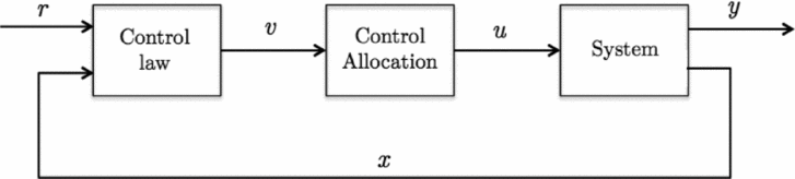
In recent years, flight control design techniques that compute the moments to be produced in pitch, roll and yaw, rather than the control surface deflections, have gained increased attention. These methods generate the virtual, or generalised, control commands, v(t), as shown in Fig. 1, that are transferred and allocated to the aircraft’s control surfaces. The problem of transforming these virtual control commands is known as the CA problem(Reference Harkegard18). Thus, the main objective of CA is to compute a control input, u(t), that ensures the commanded virtual control, v(t), is cooperatively produced by all effectors(Reference Johansen and Fossen19). The CA approach has the following features(Reference Edwards, Lombaerts and Smaili2,Reference Ducard20) ; it handles the redundancy of the control surfaces for certain optimised objectives, such as trajectory following and surface deflection prioritisation. Additionally, actuator constraints, such as rate and position limits, are taken into account in the optimisation solution. When one actuator is saturated, the other control surfaces can produce the required control efforts. Moreover, allocation problems, which are based on optimisation techniques, are of particular interest here because their computational requirements are within the capabilities of current embedded computer technology. The principles of CA, in general, are not restricted to motion control systems. Therefore, the virtual control command, v(t), is not limited to representing the generalised forces or moments, but could also represent quantities such as mass and energy(Reference Johansen and Fossen19).
CA generic scheme.

In this work, which is based on Ref. 21, a fault-tolerant constrained CA system is developed to cope with an aircraft actuator LIP fault. The developed reconfigurable approach incorporates a new control efforts redistribution process in the case of faults. Moreover, fuzzy logic scheme is implemented to correlate between the faults and control redistribution. The next section will present the techniques and formulae used in the CA problem.
2.0 MATHEMATICAL FORMULATION
2.1 CA
Consider a linear system represented by
 $$\begin{equation*}
\dot{x}(t)=Ax(t)+B_uu(t),
\end{equation*}$$
 $$\begin{equation*}
y=Cx(t)+Du(t)
\end{equation*}$$
Assume that Bu can be factorised as
 $$\begin{equation*}
B_u=B_vB,
\end{equation*}$$
where the matrix
 $B_v\in {} \mathbb {R} ^{n\times {}k}$
,
 $B\in {} \mathbb {R} ^{k\times {}m}$
, and k = rank(Bu
). Thus, the system, alternatively, can be written as:
 $$\begin{equation*}
\dot{x}=Ax+B_vv,
\end{equation*}$$
 $$\begin{equation*}
v=Bu,
\end{equation*}$$
 $$\begin{equation*}
y=Cx,
\end{equation*}$$
where
 $v\in {} \mathbb {R} ^n$
is the total required control efforts and will be referred to as the virtual control vector(Reference Harkegard22). The computation of the control law that leads to the required virtual control can be performed via different multi-variable control techniques. Allocation is the next step of the approach. CA techniques vary based on the inclusion of the actuator constraints and computational method. They are classified into two categories, unconstrained and constrained CA methods(Reference Johansen and Fossen19,Reference Petersen and Bodson23) . A comparison study between the constrained and unconstrained methods is available in Ref Reference Wang, Yi and Fan24. To allow different actuators to produce control efforts at different frequency ranges, a dynamic mapping of the following form is needed(Reference Harkegard18):
 $$\begin{equation*}
u(t)=f(v(t),u(t-T),v(t-T),u(t-2T),v(t-2T),..),
\end{equation*}$$
where T is the sampling period in seconds. The formula requires the mapping of the previous values of v and u, to capture the saturation in the actuators and penalize the actuator rates as proposed by Harkegard(Reference Harkegard25). Now, let us consider a linear dynamical model of an aircraft given by:
 $$\begin{equation*}
\dot{x}=f(x,u)
\end{equation*}$$
subject to the following position and rate constraints:
 $$\begin{equation}
u_{min}\le {}u\le {}u_{max},\ \left|{}\dot{u}\right|{}\le {}u_{rate}
\end{equation}$$
In modern aircrafts, where digital control systems are implemented, the rate constraint in Equation (1) can be transformed into position limits(Reference Durham and Bordignon26). Accordingly, the actuator rate and position limits can be written as
 $$\begin{equation}
\underline{u}(t)\le {}u\le {}\overline{u}(t),
\end{equation}$$
where
 $$\begin{equation*}
\overline{u}(t)=max[u_{min},\ u(t-T)-u_{rate}T],
\end{equation*}$$
 $$\begin{equation*}
\underline{u}(t)=min[u_{max},\ u(t-T)+u_{rate}T]
\end{equation*}$$
The Dynamic Control Allocation (DCA) task can be posed as a sequential quadratic programming problem using the Euclidean 2 nd norm(Reference Harkegard18):
 $$\begin{equation}
\Omega {}={}_{u_{min}\le {}u\le {}u_{max}}^{arg\ min}{\left\Vert {}W_v(B\ u(t)-v(t))\right\Vert {}},
\end{equation}$$
 $$\begin{equation}
u={}_{u\in {}\Omega {}}^{arg\min }{\left({\left\Vert {}W_1(u(t)-u_s(t))\right\Vert {}}^2+{\left\Vert {}W_2(u(t)-u(t-T))\right\Vert {}}^2\right)}
\end{equation}$$
where
 $B\in {} \mathbb {R} ^{k\times {}m}$
is the control effectiveness matrix,
 $u(t) \in {} \mathbb {R} ^m$
is the commanded control input,
 $v\in {} \mathbb {R}^k$
is the virtual control,
 $u_s\in {} \mathbb {R}^m$
is the desired steady-state control input, and Wv
, W
1 and W
2 are square diagonal weighting matrices of proper dimensions. When Ω is calculated, the optimisation for u(t) is made by keeping u as close as possible to the steady state value (us
), and minimising the change between the control input u(t) and the previous sampling instant u(t − T). The steady-state control input is calculated by us
(t) = Sv(t) where BS = I, and S is the control distribution matrix. In order to design a closed-loop system that fulfils the tracking requirements and control deflection constraints, the problem is then split into two main tasks. First, the virtual control command is represented in terms of the total moments generated by the actuators, subtracting the effects of the general states. The roll, pitch and yaw moments (L, M, N) are represented by their coefficients, which are functions of the control surface deflections and the aircraft states as follows:
 $$\begin{equation}
{C}_{l}= C_{l}^{\beta }\cdot \beta + C_{l}^{\delta _{a}}\cdot \delta _{a} + C_{l}^{\delta _{r}}\cdot \delta _{r} + \frac{b}{2V_{a}}(C_{l}^{p}\cdot p+C_{l}^{r}\cdot r),
\end{equation}$$
 $$\begin{equation}
C_{m}=C_{m0}+C_{m}^{\alpha }\cdot \alpha + C_{m}^{\delta _{f}}\cdot \delta _{f} + C_{m}^{\delta _{e}}\cdot \delta _{e} +\frac{c}{2V_{a}}(C_{m}^{\dot{\alpha }}\cdot {\dot{\alpha }}+ C_{m}^{q}\cdot q )+ C_{m}^{M}\cdot M,
\end{equation}$$
 $$\begin{equation}
{C}_{n}= C_{n}^{\beta }\cdot \beta + C_{n}^{\delta _{a}}\cdot \delta _{a} + C_{n}^{\delta _{r}}\cdot \delta _{r} + \frac{b}{2V_{a}}(C_{n}^{p}\cdot p+C_{n}^{r}\cdot r)
\end{equation}$$
Assuming
 $C_{m}^{\dot{\alpha }}=C_{m0}=C_{m}^{\delta _{f}}=0$
, then, the coefficients in Equation (5)–(7) are equivalently written as:
 $$\begin{eqnarray}
{\left[\begin{array}{c}C_{l}\\
C_{m}\\
C_{n} \end{array}\right]}={\left[\begin{array}{c@{\quad}c@{\quad}c@{\quad}c@{\quad}c}C_{l}^{\delta _{A-ir}}&C_{l}^{\delta _{A-il}} &C_{l}^{\delta _{A-or}} &C_{l}^{\delta _{A-ol}} &C_{l}^{\delta _{r}} \\
C_{m}^{\delta _{A-ir}} &C_{m}^{\delta _{A-il}} &C_{m}^{\delta _{A-or}} &C_{m}^{\delta _{A-ol}} &C_{m}^{\delta _{r}} \\
C_{n}^{\delta _{A-ir}} &C_{n}^{\delta _{A-il}} &C_{n}^{\delta _{A-or}} &C_{n}^{\delta _{A-ol}} & C_{n}^{\delta _{r}} \end{array}\right]} {\left[\begin{array}{c}\delta _{A-ir}\\
\delta _{A-il}\\
\delta _{A-or}\\
\delta _{A-ol}\\
\delta _{r} \end{array}\right]} \nonumber\\
+ {\left[\begin{array}{c@{\quad}c@{\quad}c@{\quad}c@{\quad}c@{\quad}c}C_{l}^{\alpha } &C_{l}^{\beta } &\frac{b}{2V_{a}}C_{l}^{p} &C_{l}^{q} &\frac{b}{2V_{a}}C_{l}^{r} &C_{l}^{M} \\
C_{m}^{\alpha } &C_{m}^{\beta } &C_{m}^{p} &\frac{b}{2V_{a}}C_{m}^{q} &C_{m}^{r} &C_{m}^{M}\\
C_{n}^{\alpha } &C_{n}^{\beta } &\frac{b}{2V_{a}}C_{n}^{p} &C_{n}^{q} &\frac{b}{2V_{a}}C_{n}^{r} &C_{n}^{M} \end{array}\right]} {\left[\begin{array}{c}\alpha \\
\beta \\
p\\
q\\
r\\
M \end{array}\right]}
\end{eqnarray}$$
Appendix A contains a table of the values of the coefficients. Thus, the virtual control will be
 $$\begin{equation}
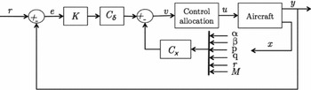
v\left(t\right)=C_{\delta}\times \delta -C_{xx},
\end{equation}$$
where C δ is the variation of moment coefficients with respect to the deflections, and δ is the actuator deflections computed by δ = e(r, y) × K. The error e is the reference error and K is a control law computed using any multi-variable design approach. This is illustrated in Fig. 2.
Illustration of the computation of the virtual control command.

Second, the virtual control command is distributed over the available effectors, which is known as the CA task. In this problem, the control command, u(t), that is feasible within the constraints of the actuator and satisfies v(t) = Bu(t), is determined at each sampling time. The S matrix is the control distribution matrix with parameters that relate to the effects of each control surface on the corresponding rotational motion. It also prioritises the role of the control surfaces.
 $$\begin{equation*}
S={\left[\begin{array}{c@{\quad}c@{\quad}c}(S_{\xi _{ir}})_{\text{roll}} & (S_{\xi _{ir}})_{\text{pitch}}&(S_{\xi _{ir}})_{\text{yaw}} \\
(S_{\xi _{il}})_{\text{roll}} & (S_{\xi _{il}})_{\text{pitch}}& (S_{\xi _{il}})_{\text{yaw}}\\
(S_{\xi _{or}})_{\text{roll}} & (S_{\xi _{or}})_{\text{pitch}}& (S_{\xi _{or}})_{\text{yaw}}\\
(S_{\xi _{ol}})_{\text{roll}} & (S_{\xi _{ol}})_{\text{pitch}}& (S_{\xi _{ol}})_{\text{yaw}}\\
(S_{\zeta })_{\text{roll}} & (S_{\zeta })_{\text{pitch}} & (S_{\zeta })_{\text{yaw}} \end{array}\right]}
\begin{array}{l}
\quad \leftarrow \text{Inner right aileron}\\
\quad \leftarrow \text{Inner left aileron}\\
\quad \leftarrow \text{Outer right aileron} \\
\quad \leftarrow \text{Outer left aileron} \\
\quad \leftarrow \text{Rudder}
\end{array}
\end{equation*}$$
In order to solve the sequential least square problem in Equation (4), it is reformulated into another form where the two cost functions are merged together, making the weighted least square problem as follows:
 $$\begin{equation}
\text{arg}\min _{\underline{u}\le u\le \bar{u}}\left\Vert W_u(u-u_p) \right\Vert ^2+\gamma \left\Vert W_v(Bu-v) \right\Vert ^2,
\end{equation}$$
where up is a preferred value of u. To emphasise the minimisation of Bu − v, the weighting factor γ will have a large value in the computation. Now, rearranging Equation (10),
 $$\begin{equation}
\left\Vert W_{u}(u-u_{p}) \right\Vert ^{2}+\gamma \left\Vert W_{v}(Bu-v) \right\Vert ^{2}= \left\Vert \underbrace{\left(\begin{array}{c}\gamma W_{v}B\\ {W_u} \end{array} \right)}_{\text{a}} u - \underbrace{\left(\begin{array}{c}\gamma W_{v}v \\ W_{u}u_{p} \end{array} \right)}_{\text{b}} \right\Vert ^{2}
\end{equation}$$
and solving for
 $$\begin{equation}
\text{arg}\min _{u}\left\Vert Au-b \right\Vert
\end{equation}$$
subject to
 $\underline{u}\le u\le \bar{u}$
. To solve Equation (12), consider
 $$\begin{eqnarray}
\min _{u}\left\Vert Au-b \right\Vert ,
\end{eqnarray}$$
 $$\begin{eqnarray}
Bu=v,
\end{eqnarray}$$
 $$\begin{eqnarray}
Cu\ge U,
\end{eqnarray}$$
where Equation (15) is equal to
 $\underline{u}(t)\le {}u\le {}\overline{u}(t)$
when
 $C=\left[\begin{array}{c}I \\ -I \end{array}\right]$
and
 $U=\left[\begin{array}{cc}\underline{u} \\ \overline{u} \end{array}\right]$
.
Given uk for the number of iterations k, find p (the optimal perturbation) such that:
 $$\begin{equation*}
\min _{p}\left\Vert A(u^k+p)-b \right\Vert
\end{equation*}$$
if uk
+ p is a feasible solution, set u
k + 1 = uk
+ p and compute
 $\left[\begin{array}{c}\mu {} \\
\lambda {} \end{array}\right]$
for which μ is associated with Bu − v and λ is associated with Equation (15). Otherwise, remove the constraints for negative λ.
The Lagrange multipliers
 $\left[\begin{array}{c}\mu {} \\
\lambda {} \end{array}\right]$
are computed from:
 $$\begin{equation*}
A^T(Au-b)={\left[\begin{array}{c}B^T\\
C_0^T \end{array}\right]} {\left[\begin{array}{c}\mu \\
\lambda \end{array}\right]},
\end{equation*}$$
where C 0 is the row of C corresponding to the constraints. This method of solving the weighted least square problem is referred to as the active set algorithm (see Ref. 27).
2.2 Reconfigurable DCA
Possible faults in actuators include LIP, hardover, loss of effectiveness and floating faults. For number of actuators m, the fault can be expressed by:
 $$\begin{equation}
u_i(t)\left\lbrace \begin{array}{l@{\quad}l}u_i(t) & \text{nominal} \\
c_i & \text{lock in place} \\
u_{i,max}&\text{hardover} \\
\rho \times u_i(t), 0< \rho < 1 & \text{loss of effectiveness } \\
0& \text{float } \end{array}\right. ,
\end{equation}$$
where i = 1,. . .,m, and ci is a fixed constant angle that represents the jammed deflection of the corresponding actuator. In this work, LIP and hardover faults are considered. The hardover is one type of LIP fault but at its maximum angle of deflection. Severe rolling motions are anticipated when the aircraft is subjected to an aileron hardover fault.
Referring back to Equation (4), the desired control input, us , is calculated by mapping the virtual control command, v(t), over the available controls using the control distribution matrix S as follows:
 $$\begin{equation*}
u_s(t)=S\ v(t)
\end{equation*}$$
Hence, in the case of any actuator fault, the distribution matrix, S, will be updated. Since the inner ailerons are symmetric and conduct essentially the same task but with opposite deflections, and similarly for the outer ailerons; only faults in the inner right aileron, outer right aileron and rudder are analysed. If any actuator is jammed, its related parameter in the S matrix will be set to zero, while other parameters will be multiplied by an updating factor, (Gf ). For a jammed inner right aileron, for instance, that affects the rolling motion, the control distribution matrix will be as follows:
 $$\begin{equation*}
S_{updated}={\left[\begin{array}{c@{\quad}c@{\quad}c}(S_{A-ir})_{roll}\times zero & (S_{A-ir})_{pitch} & (S_{A-ir})_{yaw}\\
(S_{A-il})_{roll}\times G_{f} & (S_{A-il})_{pitch} & (S_{A-il})_{yaw}\\
(S_{A-or})_{roll}\times G_{f} & (S_{A-or})_{pitch} & (S_{A-or})_{yaw}\\
(S_{A-ol})_{roll}\times G_{f} & (S_{A-ol})_{pitch} & (S_{A-ol})_{yaw}\\
(S_{A-rudder})_{roll}\times G_{f} & (S_{A-rudder})_{pitch} &(S_{A-rudder})_{yaw} \end{array}\right]}
\end{equation*}$$
The updating factor depends entirely on the fault type, magnitude and location. Due to the fact that LIP of an aileron will generate an undesirable rolling motion, it will be assumed that the magnitude of the fault will start from 0 degrees deflection. This corresponds to the scale of the updating gain factor, Gf , that starts from 1.
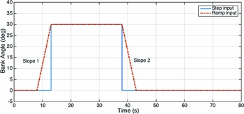
The maximum rate of change of the reference signal was also constrained because it affects how the aircraft’s actuators are excited. For instance, with a step response, the sharp change in the aircraft manoeuvre demands a faster response from the controls, which yields higher magnitudes of actuator deflection. In this FTC experiment, aircraft response was examined for two input signals, the step and ramp inputs, as shown in Fig. 3.
Step and ramp input signals.

2.3 Control Redistribution using Fuzzy Logic
Fuzzy logic is a method that can map an input space to an output space. It interpolates between sets of data of the input while keeping the provision of the most relevant output. It simplifies the knowledge acquisition while accommodating rules complexities. In this work, it is implemented to choose the updating factor for the control distribution matrix S based on data sets of faults and corresponding gains. The fuzzy sets approach was proposed in Ref. 28. Later, fuzzy logic was applied to the control of an automatic steam engine in Ref. 29. In recent years, the varieties of applications of fuzzy logic have been increasing significantly.
To implement a fuzzy logic technique, the following three steps are required(Reference Bai, Zhuang and Wang30). First, fuzzification, to convert the classical data into fuzzy data as a set of Membership Functions (MFs). Second, the Fuzzy Inference Process, which combines the membership functions with the control rules in order to get the fuzzy output. The basic classical set of operations are the intersection, union and complement(Reference Bai, Zhuang and Wang30), which can be represented by AND, OR and NOT operators, respectively, as follows:
For two classical sets, A and B, these operations can be written as:
Intersections:
 $$\begin{equation*}
A\cap {}B={\mu {}}_A\left(X\right)\cap {}\ {\mu {}}_B\left(X\right)=\min {({\mu {}}_A\left(X\right),{\mu {}}_B\left(X\right))}
\end{equation*}$$
Union:
 $$\begin{equation*}
A\cup {}B={\mu {}}_A\left(X\right)\cup {}\ {\mu {}}_B\left(X\right)=\max {({\mu {}}_A\left(X\right),{\mu {}}_B\left(X\right))}
\end{equation*}$$
Complement:
 $$\begin{equation*}
A^C=X-A,
\end{equation*}$$
where X is the entire set of elements and μ is the degree of membership. The complement of A is everything outside A. To formulate the fuzzy rules, IF-THEN processes are used. Some examples are:
For Mamdani:
IF {conditions 1} AND/OR{conditions 2}, .. AND/OR {conditions n}, THEN {output 1}, AND/OR{output 2}, .. AND/OR {output m}.
For Sugeno:
IF {Input 1 = x} and {Input 2 = y}, THEN {Output is z = ax + by + c}.
This will specify the degree to which an input data matches the condition of a rule and results in what output or action will be taken. Finally, defuzzification, which generates a table of the associated output.
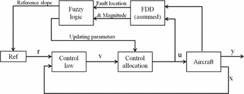
The general scheme, shown in Fig. 4, incorporates the CA system with the FTC reconfiguration, while the Fault Detection and Diagnosis (FDD) system is assumed. Information regarding faults is provided to the pre-defined fuzzy logic block that computes the reconfiguration parameters.
Reconfigurable FTCA layout.

3.0 FLIGHT CA SYSTEM FOR MULTI-AILERON AIRCRAFT
3.1 Aircraft Dynamic Model
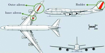
An optimal CA system is developed using a multi-effector Boeing 747 aircraft lateral dynamics model. The aircraft has two ailerons per wing (inboard and outboard) and rudder control surfaces, as shown in Fig. 5. It is assumed that engines produce fixed power; therefore, their effects due to control changes are neglected.
Boeing 747 lateral control configuration.

The twin aileron control surfaces may introduce an additional workload in the control redundancy management; however, this will give extra degrees-of-freedom for controlling the rolling motion of the aircraft, particularly under fault conditions.
At trimmed conditions of 0.8 Mach and 2500 m altitude, the linearised aircraft dynamics(Reference Alwi and Edwards31) are given by:
 $$\begin{equation*}
\dot{x}(t)=Ax(t)+Bu(t)
\end{equation*}$$
 $$\begin{equation*}
y(t)=Cx(t)+Du(t),
\end{equation*}$$
where
 $$\begin{eqnarray*}
A&=&{\left[\begin{array}{c@{\quad}c@{\quad}c@{\quad}c}-1.06 &0.172 &-1.65 &0.0004 \\
-0.12 & -0.21 &0.28 &-0.002 \\
0.1014 &-0.989 &-0.1 &0.106 \\
1 &0.09 &0 &0 \end{array}\right]} \\
B&=&{\left[\begin{array}{c@{\quad}c@{\quad}c@{\quad}c@{\quad}c}-0.083 &0.083 &-0.2285 &0.2285 &0.1187 \\
-0.0154 & 0.0154 &-0.0123 & 0.0123 &-0.2478 \\
0 &0 &0 &0 &0.0174 \\
0 & 0 & 0 & 0 & 0 \end{array}\right]}
C={\left[\begin{array}{c@{\quad}c@{\quad}c@{\quad}c}0 &0 &1 &0 \\
0 & 0 & 0 & 1 \end{array}\right]}
\end{eqnarray*}$$
and D is a (2 × 5) zero matrix. The states vector x = [p r β ϕ] T comprises the roll rate (rad/s), yaw rate (rad/s), sideslip angle (rad) and the roll angle (rad) consecutively. The control input vector u = [ξ ir ξ il ξ or ξ ol ζ] T consists of the inboard right and left ailerons, outboard right and left ailerons, and the rudder, respectively. Measured outputs y(t) represent the sideslip angle, β, and the roll angle, ϕ. The aircraft’s main effectors for lateral control are shown in Fig. 5. Maximum deflection of the actuators is ± 30°, and the maximum rate of change is ± 50° per second.
3.2 The Flight Control Law
The control law, that yields the virtual control command v(t), based on Equation (9), is designed first in the CA problem. An H ∞ controller is developed to utilise the optimising features of minimising the tracking error and total control energy. For a closed-loop system, the control law problem is represented by finding an optimal stabilising solution that minimises the following cost function:
 $$\begin{equation}
{\left\Vert {}\begin{array}{c@{\quad}c}W_e{(I+GK)}^{-1} \!\!\!\!\! \\
{W_uK(I+GK)}^{-1} \!\!\!\!\!\!\end{array}\right\Vert {}}_{\infty {}}
\end{equation}$$
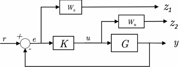
for the feedback control law shown in Fig. 6.
Closed-loop system with the weight minimisation functions.

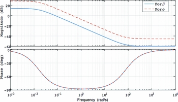
The weighting functions W e and W u are used to shape the output [z 1 z 2] T , for the tracking error and control input minimisation. To minimise the tracking error of the sideslip and roll angles [β ϕ] T , the weighting function We is a diagonal matrix with two low-pass filters that minimise the two reference inputs. The filter will allow signals with frequencies less than the cross-over frequency to pass, but attenuate signals with frequencies higher than the cross-over frequency.
The weighting function We for the roll angle, ϕ, is higher in magnitude than the one for sideslip angle, β, to give it more significance in the optimisation problem as shown in the Bode plot of Fig. 7.
We weighting functions for ϕ and β.

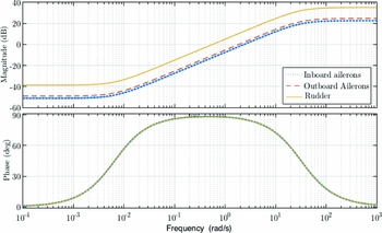
The second weighting function in the H∞ control law design is Wu . This function is used to shape the controlling efforts of the actuators. Three main sets of controls, namely the inboard ailerons, outboard ailerons and the rudder, are available. The primary roll effectors are the outer ailerons. Weights given to each effector are correlated to its primary task. In Fig. 8, the Bode plot shows the weighting function Wu , for the control inputs.
Wu functions for aircraft’s control surfaces.

A Matlab algorithm is used to compute the stabilising solution that minimises the cost function in Equation (17). Results of the tuning and computations yields the optimal stabilising solution with γ = 0.998, and H∞ control gain in the state-space form as shown in Appendix B.
3.3 The Total Virtual Control Command
For the aircraft with 211 ft span and 33 ft chord, the virtual control command is computed following the scheme depicted in Fig. 2. Aerodynamic stability and control derivatives are listed in Appendix A. Using these parameters, the matrices in the system are found as follows:
 $$\begin{equation*}
C_\delta ={\left[\begin{array}{c@{\quad}c@{\quad}c@{\quad}c@{\quad}c}-0.013 &0.013 &-0.017 &0.017 &0.004 \\
0 &0 &0 &0 &0 \\
-0.0015 &0.0015 &-0.0012 &0.0012 &-0.108 \end{array}\right]}
\end{equation*}$$
and
 $$\begin{equation*}
C_x={\left[\begin{array}{c@{\quad}c@{\quad}c@{\quad}c@{\quad}c@{\quad}c}0 & -0.193 & -0.0101 & 0 &0.0067 &0 \\
-1.15& 0 & 0 &-0.1461 &0 &0.12 \\
0& 0.147 & -0.002 & 0 & -0.0067 & 0 \end{array}\right]},
\end{equation*}$$
where
 $$\begin{equation*}
x(t)={\left[\begin{array}{c@{\quad}c@{\quad}c@{\quad}c@{\quad}c@{\quad}c}\alpha & \beta & p & q & r & M \end{array}\right]} ^{T}
\end{equation*}$$
Detailed aerodynamic characteristics for the B747 are available in Refs 32 and 33. The resulting computed virtual control command, v(t), is composed of three vectors that represents the total required control efforts along the roll, pitch and yaw axes.
3.4 CA
Once the virtual control command, v(t), is computed, the task of allocating the total control efforts to the available aircraft control surfaces can begin. In trimmed flight, the weighting factors of the steady-state control distribution matrix (S) that resembles the relationships between total required rolling, pitching and yawing efforts and the corresponding control surfaces are chosen to be:
 $$\begin{equation*}
S={\left[\begin{array}{l@{\quad}l@{\quad}l}-5.0 &-0.05 &-0.12 \\
5.0& -0.05&0.12 \\
-10&-0.02 &-1.0 \\
10&-0.02 &1.0 \\
0.02& 0&-8.0 \end{array}\right]}
\end{equation*}$$
This matrix considers the priorities among the three moments and also the contribution factors of each control surface. The weights to shape the tracking error and control energy in the optimisation cost function are
 $W_e=\text{diag} \ ([2\ 2\ 2\ 2\ 2])$
and
 $W_u=\ \text{diag}([8\ 8\ 10\ 10\ 10])$
.
3.5 Constrained DCA
In this computation method, the control input, u(t), is calculated based on the virtual control command optimisation function, using a weighted least-squares solver(Reference Harkegaard27). Thus, in order to give more emphasis on the virtual control commands that generates the rolling motion, the weights corresponding to the pitching and yawing motions are kept small,
 $Wv=\text{diag}([10\ 1\ 1])$
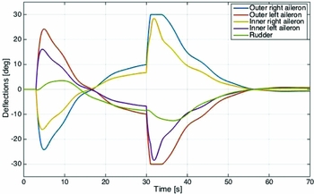
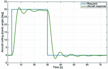
. Results of using the constrained DCA technique are shown in Fig. 9 for controls deflections and in Fig. 10 for aircraft response. The deflection plot shows high rate of change (reaching 20°/s) in the controls, yielding a faster aircraft response. Moreover, the deflections were constrained by the maximum deflection angle limits. It is shown that when one actuator saturates, the other actuators remaining margin of deflection is exploited.
Control surface deflections using constrained DCA.

Aircraft response using DCA.

The aircraft response is fast (rise time is 2.8 seconds) and well damped, resulting in a relatively small steady-state error (<3%).
4.0 RECONFIGURABLE CA AGAINST FAULTS
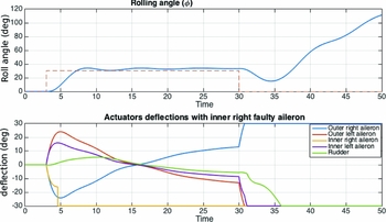
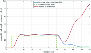
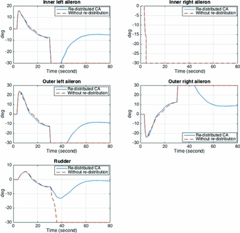
In this work, LIP and hardover faults are considered. The hardover fault is one type of LIP fault, but it occurs at its maximum deflection angle. Severe rolling motions are anticipated when the aircraft is subjected to an aileron hardover fault. The previously developed nominal constrained CA system was subjected to this fault, and the results are shown in Fig. 11. The inner right aileron of the aircraft is assumed to encounter the hardover fault 1 second after the pilot’s roll input command. The available healthy control surfaces cooperate to accommodate the fault and deliver the required roll angle response. However, all actuators were driven to saturation when the pilot requests a roll back to a 0° angle, i.e. wing level. This is due to the accumulative efforts passed to each control surface which results in a drastically unstable roll motion of the aircraft.
Roll motion and deflections when inner right aileron is subjected to a hardover fault.

The result highlights that the aircraft’s controls are to be reconfigured to overcome the deficiency of the available control surfaces in order to gain stable and safe flight. Since the actuators in the DCA optimisation problem were driven to their maximum rate of change in the design process before the fault, changes in the weights We and Wv will not have significant impacts unless the tracking accuracy is reduced. Therefore, the adjustment of the control distribution matrix will be investigated in order to reshape the efforts directed to the available control surfaces in the presence of a fault.
4.1 Redistribution of the Control Efforts
The desired control input, us , is calculated by mapping the virtual control command, v(t), over the available control effectors using the control distribution matrix S as follows:
 $$\begin{equation*}
u_s(t)=S\ v(t)
\end{equation*}$$
Hence, in the case of any actuator fault, the distribution matrix S is to be updated. Since the inner ailerons are symmetric and conduct essentially the same task but with opposite deflections, and similarly for the outer ailerons, only faults in the inner right aileron, outer right aileron and rudder are analysed. If any actuator is jammed, its related parameter in the S matrix will be set to zero, while other parameters will be multiplied by an updating factor, (Gf ). For a jammed inner right aileron, for instance, that affects the rolling motion, the control distribution matrix will be as follows:
 $$\begin{equation*}
S_{updated}={\left[\begin{array}{c@{\quad}c@{\quad}c}(S_{A-ir})_{roll}\times zero & (S_{A-ir})_{pitch} & (S_{A-ir})_{yaw}\\
(S_{A-il})_{roll}\times G_{f} & (S_{A-il})_{pitch} & (S_{A-il})_{yaw}\\
(S_{A-or})_{roll}\times G_{f} & (S_{A-or})_{pitch} & (S_{A-or})_{yaw}\\
(S_{A-ol})_{roll}\times G_{f} & (S_{A-ol})_{pitch} & (S_{A-ol})_{yaw}\\
(S_{A-rudder})_{roll}\times G_{f} & (S_{A-rudder})_{pitch} &(S_{A-rudder})_{yaw} \end{array}\right]}
\end{equation*}$$
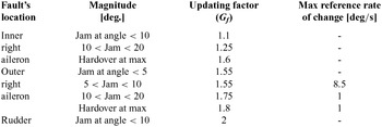
If the fault occurs in the rudder, the third column represents the yaw moment will be updated. The updating factor depends entirely on the fault type, magnitude and location. Table 1 summarises the selected Gf for the system when LIP fault occurs in the lateral control surfaces, either the ailerons or rudder. The selection depends on how severe is the fault and on which control surface.
Selected updates to the system subjected to actuator LIP faults

4.2 Fuzzy Logic Implementation
Fuzzy inference-related calculations are performed prior to the real application. Therefore, it is not a time-consuming process when it is run online. It is implemented using the Matlab/Simulink software. Sugenos fuzzy logic method is computationally more efficient and has a more compact representation than a Mamdani system(Reference Wang34). Thus, it is selected in this work. The inputs are the location and magnitude of the fault, while the outputs are the control distribution update factors and the input signals maximum rate of change. The membership functions were designed based on the set of classical input data, which is the fault location and magnitude with a multivalued logic that represents the intersection operation. The set of rules combined the updating factors (listed in Table 1) with these functions to shape the required output.
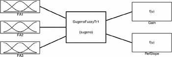
As shown in Fig. 12, the fuzzy system comprises three inputs, FA1 , FA2 and FA3, that represent the inner right aileron fault, the outer right aileron fault and the rudder fault, respectively.
Fuzzy logic using Sugeno’s model.

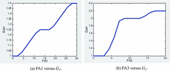
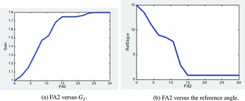
Results of the rules are illustrated by the plots for the updating gains associated with each fault’s magnitude, as shown in Fig. 13 for inner aileron and rudder against the updating factor, while Fig. 14 shows the plots for FA2 against the updating factor and the required maximum slope for reference angle.
Inner FA1 and rudder FA3 faults versus updating factor Gf .

Outer aileron faults FA2 versus updating factor Gf and reference angle.

5.0 SIMULATION RESULTS
LIP and hardover faults have been considered in this work. In all scenarios, it was assumed that fault information was provided 1 second after the fault occurs, and redistribution was conducted directly afterwards. The testing was conducted for a number of fault magnitudes.
5.1 Inner Right Aileron Faults
5.1.1 LIP fault
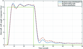
The fault was introduced to the inner right aileron while the opposite inner left aileron was assumed to be working properly. In this experiment, the actuator stuck at an angle of 17° at time t=3 seconds. The aircraft response (in Fig. 15) shows how the redistributed and nominal CA dealt with this situation. The difference between the two was small, where both optimal computations yielded a good rise time (3 seconds) and less than 10% overshoot. The redistributed CA produced a slightly faster settling time response, and both introduced a very small settling error (<2°).
Response with jammed inner right aileron at 17°.

Control deflections are shown in Fig. 16, where the redistributed CA had introduced a very small difference in the deflection compared to the nominal. This was due to the small influences of secondary effects produced by the inner ailerons on the roll motion.
Aircraft control deflections with 17°
LIP fault on the inner right aileron.

5.1.2 Hardover fault
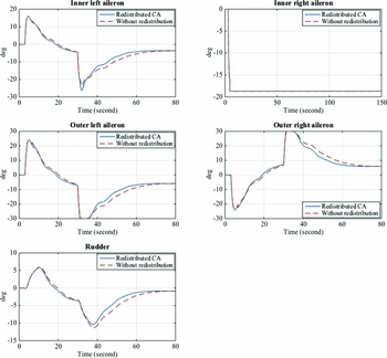
The aircraft response to a hardover fault on the inner right aileron is shown in Fig. 17. The normal CA without redistribution was unable to maintain control of the aircraft, and resulted in a deterioration of aircraft stability. On the other hand, the redistribution of control efforts preserved stability and led to an improved tracking response with small settling error (<3°).
Aircraft response with hardover fault on the inner right aileron.

Control surface deflections resulting from this situation are shown in Fig. 18, where in the nominal distribution case, all the available healthy actuators were driven to their maximum deflections (i.e. saturation) in order to restore stability but without success. However, when using the redistributed CA technique, the system accommodated the fault and the actuators were optimised for successful deflection performance against the step input signal.
Control surface deflections with hardover fault on the inner right aileron.

5.2 Outer Right Aileron Faults
The outer ailerons are considered to be the primary effectors for roll control. Hence, any LIP fault will affect stability and tracking performance of the aircraft. The controllability of the aircraft will be tested only using the developed FTCA approach.
5.2.1 10° LIP fault
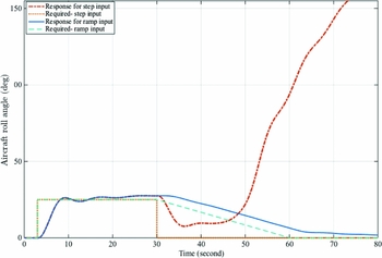
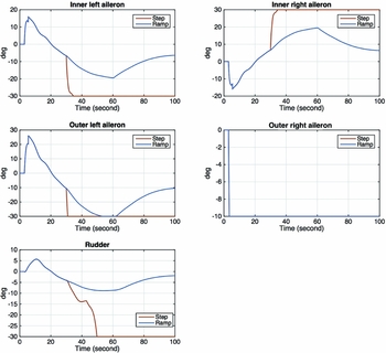
This fault scenario, as shown in Fig. 19, yielded an unstable aircraft response when the redistributed CA was subjected to a step input. Redistribution of control efforts achieved a stable response only when the ramp input was applied. This led to a substantial limitation in the roll rate. Although this trajectory is a slow-moving signal, the developed CA was able to guarantee the stability and automatic tracking performance of the system.
Response for step and ramp inputs, with 10°
LIP fault in outer right aileron.

Control surface deflections for the 10° LIP fault in the outer right aileron are shown in Fig. 20, where the step input resulted in saturation of all the available actuators and hence led to the aforementioned unstable aircraft response. On the other hand, the LIP fault in the outer right aileron was accommodated when a ramp input was applied, which resulted in smooth actuator deflections.
Deflections for step versus ramp inputs.

5.2.2 16° LIP fault
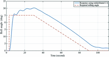
At higher magnitudes of LIP faults occurring in the outer right aileron, the aircraft was pushed to the edge of tracking performance and stability. A 16° jam fault was introduced at t=5 seconds, and through the redistribution of the control efforts, the system was just able to meet the stability conditions when the constrained ramp input was applied, as shown in Fig. 21.
Bank angle response for 16°
LIP fault on outer right aileron.

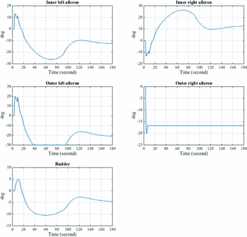
Control surface deflections for the redistributed CA using the constrained ramp input are shown in Fig. 22. As a result of the selected reference input, the deflections are smooth and maintain the actuator’s limits of position and rate of change.
Deflections with 16°
LIP in the outer right aileron.

The magnitude of the fault on the outer right aileron was analysed further. Faults with large magnitudes drastically affect the stability of the aircraft and lead to uncontrollable aircraft manoeuvres, which are considered to be at the limits of this control’s ability to restore the stability of the aircraft.
5.3 Rudder Faults
As discussed previously, the yawing motion of the aircraft is mainly controlled by the rudder. Thus, in the case of LIP faults, the available ailerons deflection will be required to overcome this problem and maintain the stability and tracking performance.
5.3.1 6° LIP fault
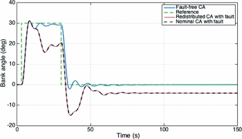
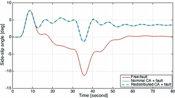
When the rudder jammed at 6° of deflection, the aircraft in both redistributed and nominal CA cases had a similar stable response, as shown in Fig. 23. There was an overshoot and an acceptable 4° steady-state error in the bank angle.
Aircraft bank angle response against 6° LIP fault on the rudder.

The sideslip angle (β) response in Fig. 24 shows that, in the free-fault case, the controller minimised the angle to 0°. With faults in the rudder, there was a 4° induced sideslip angle, with the aircraft brought back to straight flying. There was no improvement in the response due to redistribution; however, the CA optimal control yielded a minimum divergence of the sideslip angle.
Aircraft sideslip angle response with 6° LIP fault on the rudder.

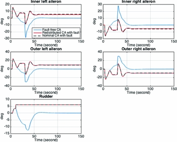
Aircraft actuator deflections, when the aircraft was subjected to a 6° jammed rudder, are shown in Fig. 25. In the control distribution matrix S, updating the elements of the available healthy actuators, corresponding to the rolling and yawing rotation, has not yielded any improvements compared to the nominal CA response. This was due to the fact that the contributions from the ailerons are relatively small compared to the rudder. Nevertheless, in general, the DCA led to a stable response.
Deflections with 6° LIP fault on the rudder.

5.3.2 10° LIP fault
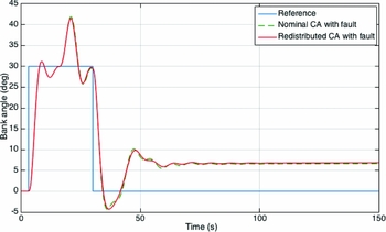
When applying a 10° LIP fault to the rudder, the nominal CA matched the redistributed CA, as shown in Fig. 26. The optimal solution of the CA managed to maintain the stability of the aircraft, with an increase in the overshoot and settling tracking error as the LIP fault on the rudder increases.
Aircraft response when the rudder is jammed at 10°.

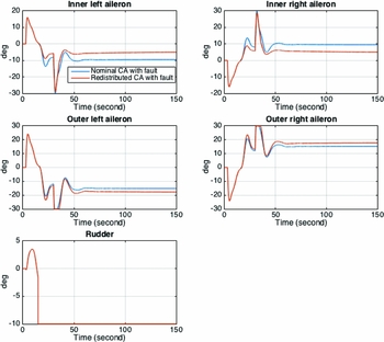
The related deflections are shown in Fig. 27. Although the redistributed CA excited the available controls, there was no difference in the aircraft’s response. This was due to the limited influence of the ailerons towards the compensation of rudder faults.
Deflections with 10° LIP rudder fault.

6.0 CONCLUSION
This paper discusses the development of a reconfigurable fault-tolerant flight control system for a multi-effector aircraft using a CA technique and a new method of distributing control effort amongst the control surfaces. The aircraft model used in the study has redundant ailerons and a rudder as the primary control inputs for lateral motion. An optimal CA problem that handles the redundancy of the control surfaces, tracking requirements, and actuator constraints was formulated. The control input constraints include both the maximum rate of change and the saturation limits. The developed approach incorporates a new control redistribution process, which is updated on the occurrence of a fault. This approach relies on and assumes an effective on-board FDD system to provide precise information regarding the actuator fault. Fuzzy logic was implemented to correlate between the faults and the control redistribution. The fuzzy logic implementation handles a wide range of fault magnitudes on-line, by interpolation. The system deals with a severe type of actuator fault, which is the LIP fault.
When the inner aileron experienced an LIP fault of 20° or less, the system was asymptotically stabilised using both the baseline and reconfigured CA methods. This was due to the minor effects brought about by the inner ailerons on the rolling motion. Hardover faults, on the other hand, deteriorated the tracking performance as the control surfaces were driven to saturation using the baseline CA. Nevertheless, the system was stabilised against this fault using the redistributed CA, where the tracking performance and control deflection constraints were fulfilled.
As the primary roll effector, LIP faults on the outer aileron had a significant influence on the aircraft response. In this case, stability was only retained when using the redistributed CA and the ramp input on the bank angle, with the rate of change depending on the magnitude of the fault. Higher than 16% LIP faults on the outer aileron could not be alleviated with the proposed settings, due to the saturation limits of the available healthy actuators. Finally, in the case of rudder faults, the redistribution of control efforts to the ailerons to accommodate jammed rudder faults did not improve the aircraft response. However, the system was stable using the CA scheme, with some degradation in tracking performance.
For further work, the linear-based controller could be tested in a non-linear environment. Moreover, improvement of the tracking performance is suggested to overcome the problem of outer aileron faults with a large magnitude. Engine thrust could be integrated into the control loop. Additionally, the effects of delays introduced by the FDD could be also investigated.
APPENDIX
A.0 STABILITY AND CONTROL DERIVATIVES
The Boeing 747 stability and control derivatives are as follows:
 \fontsize{9}{10}\selectfont{$$\begin{eqnarray*}
{\begin{array}{c@{\quad}c}C_{l}^{\beta } &-0.193 \\
C_{l}^{p} & -0.3 \\
C_{l}^{r} & 0.2 \\
C_{m}^{\alpha } &-1.15 \\
C_{m}^{q} &-20 \\
C_{m}^{M} & 0.12 \\
C_{n}^{\beta } & 0.147 \\
C_{n}^{p} & -0.06 \\
C_{n}^{r} & -0.2 \\
& \\
C_{l}^{\delta _{A-ir}} &-0.013 \\
C_{l}^{\delta _{A-il}} & 0.013 \\
C_{l}^{\delta _{A-or}} &-0.017 \\
C_{l}^{\delta _{A-ol}} & 0.017 \\
C_{l}^{\delta _{R}} & 0.004 \\
C_{m}^{\delta _{A-ir}} & 0 \\
C_{m}^{\delta _{A-il}} & 0 \\
C_{m}^{\delta _{A-or}} & 0 \\
C_{m}^{\delta _{A-ol}} & 0 \\
C_{m}^{\delta _{R}} & 0 \\
C_{n}^{\delta _{A-ir}} &-0.0015 \\
C_{n}^{\delta _{A-il}} & 0.0015 \\
C_{n}^{\delta _{A-or}} &-0.0012 \\
C_{n}^{\delta _{A-ol}} & 0.0012 \\
C_{n}^{\delta _{R}} & -0.108 \\
\end{array}}
\end{eqnarray*}$$}
B.0 STATE SPACE MODEL FOR H∞ CONTROL FOR THE CONTROL ALLOCATION
 \fontsize{6.9}{8.9}\selectfont{$$\begin{equation*}
A={\left[\begin{array}{c@{\;\;\,}c@{\;\;\,}c@{\;\;\,}c@{\;\;\,}c@{\;\;\,}c@{\;\;\,}c@{\;\;\,}c@{\;\;\,}c@{\;\;\,}c@{\;\;\,}c}-5.245 &-7.964 &6.102 &-7.64 &-0.1896 &3.292 &1.282 &-1.282 &2.466 &-2.466 &0.4922 \\
-0.5266 &-1.004 &1.032 &-0.747 &-0.01895 &0.3208 &0.0993 &-0.0993 &0.2694 &-0.2694 &-0.1726 \\
0.1066 &-0.9782 &-0.1096 &0.1151 &0.00027 &-0.004131 &-0.002044 &0.002044 &-0.003951 &0.003951 &0.01431 \\
1 &0.09 &0 &0 &0 &0 &0 &0 &0 &0 &0 \\
0 &0 &0 &0 &-0.0158 &0 &0 &0 &0 &0 &0 \\
0 &0 &0 &0 &0 &-0.0158 &0 &0 &0 &0 &0 \\
42.68 &83.02 &-78.99 &77.89 &1.944 &-33.55 &-16.18 &16.18 &-31.81 &31.81 &-4.051 \\
-42.68 &-83.02 &78.99 &-77.89 &-1.944 &33.55 &16.18 &-16.18 &31.81 &-31.81 &4.051 \\
83.72 &162.7 &-155 &152.8 &3.792 &-65.82 &-31.69 &31.69 &-62.38 &62.37 &-7.791 \\
-83.72 &-162.7 &155 &-152.8 &-3.792 &65.82 &31.69 &-31.69 &62.38 &-62.37 &7.791 \\
11.2 &22.36 &-20.75 &20.51 &0.5716 &-8.813 &-4.361 &4.361 &-8.429 &8.429 &-1.502
\end{array}\right]}
\end{equation*}$$}
 \fontsize{9}{10}\selectfont{$$\begin{equation*}
B={\left[\begin{array}{c@{\;\;\,}c}0 & 0 \\
0 & 0 \\
0 & 0 \\
0 & 0 \\
7.025 & 0 \\
0 & 7.025 \\
0 & 0 \\
0 & 0 \\
0 & 0 \\
0 & 0 \\
0 & 0 \end{array}\right]}
\end{equation*}$$}
 \fontsize{7}{9}\selectfont{$$\begin{equation*}
C={\left[\begin{array}{c@{\;\;\,}c@{\;\;\,}c@{\;\;\,}c@{\;\;\,}c@{\;\;\,}c@{\;\;\,}c@{\;\;\,}c@{\;\;\,}c@{\;\;\,}c@{\;\;\,}c}0.6903&1.343&-1.278&1.26&0.03144&-0.5428&0.2565&0.2617&-0.5145&0.5145&-0.06554 \\
-0.6903&-1.343&1.278&-1.26&-0.03144&0.5428&0.2617&0.2565&0.5145&-0.5145&0.06554 \\
1.064&2.067&-1.969&1.942&0.04819&-0.8366&-0.4028&0.4028&-0.3856&0.7927&-0.09902\\
-1.064&-2.067&1.969&-1.942&-0.04819&0.8366&0.4028&-0.4028&0.7927&-0.3856&0.09902\\
0.04294&0.08573&-0.07959&0.07866&0.002192&-0.03379&-0.01672&0.01672&-0.03232&0.03232&0.1171 \end{array}\right]}
\end{equation*}$$}
 \fontsize{9}{10}\selectfont{$$\begin{equation*}
D={\left[\begin{array}{c@{\quad}c}0 & 0 \\
0 & 0 \\
0 & 0 \\
0 & 0 \\
0 & 0 \end{array}\right]}
\end{equation*}$$}