1. Introduction
Turbulent entrainment (Townsend Reference Townsend1976) is a fundamental process governed by local conditions of the moving turbulent/non-turbulent interface – the viscous ‘superlayer’ – as well as other non-local factors. The superlayer is characterised by an approximate balance of turbulent advection of energy and its viscous diffusion, the equivalent physical processes having been described, respectively, as ‘engulfment’ (Turner Reference Turner1986) and ‘nibbling’ (Corrsin & Kistler Reference Corrsin and Kistler1955). Modern experimental techniques have enabled study of the relative importance of these fundamental processes involved in vorticity transport (Westerweel et al. Reference Westerweel, Kukushima, Pedersen and Hunt2005; Philip & Marusic Reference Philip and Marusic2012): they are key in controlling the growth rates of free shear layers and therefore the reactive forces on the solid bodies producing them. Control of entrainment can therefore make many fluid-based systems more efficient: for example, its reduction in the wake of a bluff body will reduce the pressure (or ‘form’) drag of that body. Here, we report a phenomenon in which a high-frequency jet is used to increase the base pressure of a bluff body from which separation occurs at a sharp trailing edge. Given that the drag of such a body is dominated by pressure drag, there is an associated reduction in the wake momentum flux deficit.
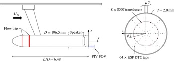
A recent review of the subject by Choi, Jeon & Kim (Reference Choi, Jeon and Kim2008) includes techniques that are either passive (for example, Strykowski & Sreenivasan Reference Strykowski and Sreenivasan1990; Heenan & Morrison Reference Heenan and Morrison1996, Reference Heenan and Morrison1998; Parezanovic & Cadot Reference Parezanovic and Cadot2012) or active (Zaman & Hussain Reference Zaman and Hussain1981; Gaster, Kit & Wygnanski Reference Gaster, Kit and Wygnanski1985; Kim & Choi Reference Kim and Choi2005; Vukasinovic, Rusak & Glezer Reference Vukasinovic, Rusak and Glezer2010), the latter with or without feedback (Kang & Choi Reference Kang and Choi2002; Dahan, Morgans & Lardeau Reference Dahan, Morgans and Lardeau2012). Effective direct-wake control (as opposed to separation delay), whether in open or closed loop, requires an understanding of the large-scale organised structures and their interaction. These are geometry-specific: in the present study, we apply pulsed-jet blowing to the near-wake of an axisymmetric body, its axis aligned with the free-stream direction, and where turbulent separation occurs at a sharp trailing edge, immediately beneath which there is a small annular slit through which the jet emerges parallel to the free stream: see figure 1.
Schematic of the experimental model and PIV fields of view.

We initially reported a significant pressure recovery (Morrison & Qubain Reference Morrison, Qubain and Eckhardt2009; Qubain Reference Qubain2009; Qubain & Morrison Reference Qubain and Morrison2009) over a narrow range of frequencies (at about five times the shear layer frequency) without a detailed understanding of how it occurs. The effect is generic in that it has been demonstrated for turbulent flow over a backward-facing step (Qubain Reference Qubain2007) as well as a bluff body of rectangular cross-section (Cabitza Reference Cabitza2013; Barros et al. Reference Barros, Ruiz, Borée and Noack2014). Although the jet is of zero net-mass flux (Glezer & Amitay Reference Glezer and Amitay2002), we avoid the term ‘synthetic’ jet because, as we show below, a time-averaged jet is not produced by the self-induced velocity of a vortex ring pair. We further observe that, crucially, the nonlinear coupling between the jet and the wake requires there to be a finite, jet-induced momentum flux which manifests itself as a change in pressure drag on the body. Here we show that a global instability can be controlled indirectly from a location where the separating boundary layer is convectively unstable, or where an ‘amplifier’ is receptive to ‘extrinsic’ disturbances (Huerre Reference Huerre, Batchelor, Moffatt and Worster2000).
A full description of the unforced wake in the present experiment is provided by Rigas et al. (Reference Rigas, Oxlade, Morgans and Morrison2014b ), who show that the coherent structures of the turbulent wake retain the symmetry-breaking properties of the laminar wake. Similarly, oscillatory bifurcations appearing at low Reynolds numbers (the ones at higher Reynolds numbers breaking reflectional symmetry) also appear in the turbulent wake as axisymmetric ‘bubble pumping’ (Berger, Scholz & Schumm Reference Berger, Scholz and Schumm1990) and as ‘vortex shedding’ (Achenbach Reference Achenbach1974; Taneda Reference Taneda1978; Fuchs, Mercker & Michel Reference Fuchs, Mercker and Michel1979; Berger et al. Reference Berger, Scholz and Schumm1990), a large-scale antisymmetric oscillation. This has often been referred to as a ‘helical’ mode when, in fact, as shown by Rigas et al. (Reference Rigas, Oxlade, Morgans and Morrison2014b ), periodic shedding is perturbed by a random variation of the azimuthal shedding angle on a very long time scale. They further show that, in a statistical sense, the broken symmetries are restored at much higher Reynolds numbers (Rigas et al. Reference Rigas, Morgans, Brackston and Morrison2014a ).
Monkewitz (Reference Monkewitz1988) conducted a linear stability analysis for a family of axisymmetric wake (parallel flow) profiles: he showed that this asymmetric mode is absolutely unstable, and in agreement with experimental observation by Taneda (Reference Taneda1978), he noted that it is most clearly observed somewhat downstream of the body. Grandemange, Gohlke & Cadot (Reference Grandemange, Gohlke and Cadot2013) show that these characteristics are consistent with those of a wake from a three-dimensional body of rectilinear geometry. Ho & Huerre (Reference Ho and Huerre1984) have identified the boundary layer momentum thickness,
 ${\it\theta}$
, as the appropriate length scale. A linear stability analysis of an initially laminar, plane mixing layer shows that maximum amplification occurs at Strouhal number
 $\mathit{St}_{{\it\theta}}=f{\it\theta}/U_{\infty }=0.016$
. For a turbulent separation, maximum amplification occurs at
 $\mathit{St}_{{\it\theta}}=0.022{-}0.024$
(Zaman & Hussain Reference Zaman and Hussain1981; Ho & Huerre Reference Ho and Huerre1984).
2. Experimental details
Figure 1 shows a schematic of the model which is mounted in a closed-circuit wind tunnel, the working section of which measures
 $1.37~\text{m}\times 1.22~\text{m}\times 3.0~\text{m}$
. The contraction ratio is 4.92:1 and the free-stream turbulence intensity is less than 0.1 %. A proportional-integral-derivative (PID) controller with a set-point variation of less than 0.2 % is used to maintain the free-stream velocity
 $U_{\infty }=15~\text{m s}^{-1}$
(Reynolds number based on diameter of
 $\mathit{Re}_{D}=1.88\times 10^{5}$
, and at separation,
 $\mathit{Re}_{{\it\theta}}=2050$
). The leading edge is a modified super-ellipse with an aspect ratio of 2.5. The boundary layer is conditioned in two stages: the first is a 2 mm wide strip of 120 grit emery paper located at approximately the point of minimum surface pressure; the second is a 25 mm wide strip of 120 grit emery paper which serves to thicken the boundary layer. The boundary layer at separation was checked by a full traverse of about 50 data points: it shows an approximate log law region from which a wall friction velocity of
 $u_{{\it\tau}}=0.68~\text{m s}^{-1}$
is estimated. The shape factor
 $H=1.34$
.
A high-fidelity speaker mounted inside the model is used to generate a pulsed jet of variable frequency and amplitude. The jet issues in the free-stream direction from a 2.0 mm wide annular slit, located 1.0 mm below the trailing edge. The choice of slit width was based on preliminary measurements and chosen to match the boundary layer momentum thickness,
 ${\it\theta}=2.14~\text{mm}$
. In order that jet disturbances are amplified as much as possible, the slit was placed as close as possible to the point of separation. A BEYMA 6MI100 mid-range driver was chosen for its high sensitivity (97 dB) and nominal power rating (250 W) to maximise the parameter space over which the pressure recovery can be studied. A harmonic forcing signal is generated by the control code and converted to an analogue signal by the 16 bit D/A converter sampling at 800 kHz. A QSC RMX 850 high-fidelity power amplifier drives the loudspeaker. The jet velocity was calibrated with a single hot wire against speaker-chamber pressure, the amplitude of which was also maintained constant using a PID controller, with a set-point variation for the speaker-chamber pressure of less than
 $0.15\,\%$
. The jet centre-line velocity,
 $u_{f}$
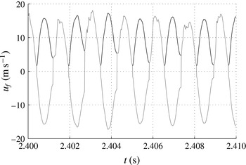
, is quantified in quiescent flow using a hot wire placed at the orifice. Figure 2 shows the unrectified signal which is de-rectified by a simple peak/trough detection algorithm;
 $u_{j}$
is defined as the amplitude of the Fourier component of the jet centre-line velocity at the forcing frequency. This measure is preferable to one based solely upon the peak jet velocity (as used by Qubain Reference Qubain2009). Firstly, it distinguishes between the flux at the forcing frequency and other frequency components which occur at larger forcing amplitudes: see figure 2. Secondly, the hot wire rectifies the velocity with an unknown sensitivity to negative velocities. Since it is difficult to distinguish the efflux (blowing) from influx (suction), use of a Fourier amplitude reduces the uncertainty associated with the mis-identification of suction peaks. At forcing amplitudes used in this experiment, the jet turbulence intensity (as a deviation from a pure sinusoid) is less than 2.5 %.
Measurement of the jet centre-line velocity:
 $u_{f}$
(black line), raw;
 $u_{j}$
(grey line), de-rectified Fourier amplitude.

The forcing amplitude is defined by
 $$\begin{eqnarray}C_{{\it\mu}}=\frac{u_{j}^{2}A_{j}}{U_{\infty }^{2}A},\end{eqnarray}$$
where
 $A_{j}$
is the area of the jet orifice, and
 $A$
is the area of the base of the model. Considerations of self-similarity imply that the jet momentum flux depends on
 $(u_{j}-U_{\infty })$
. However,
 $U_{\infty }$
is fixed in this experiment and for simplicity, therefore,
 $C_{{\it\mu}}$
is defined by (2.1).
The model base is instrumented with 64 static pressure tappings (connected to a 64 channel ESP-DTC pressure scanner) and 11 Endevco 8507C pressure transducers (only 8 are shown in figure 1) which were sampled at, respectively, 225 Hz and 40 kHz. At each forcing condition, pressure data were acquired for a total of 480 s over 8 independent experiments, providing a 95 % uncertainty of approximately 6 % and 13 % for the mean and variance of pressure respectively. Pressure measurements are expressed as a pressure coefficient, non-dimensionalised by the free-stream dynamic head.
Random and phase-locked two-component particle image velocimetry (PIV) measurements were performed immediately downstream of the jet orifice on the upper and lower separating shear layers simultaneously. A conservative estimate of the PIV spatial resolution, the
 $-3~\text{dB}$
cut-off wavenumber of the PIV measurement, gives a cut-off wavelength,
 ${\it\lambda}_{c}=0.7~\text{mm}$
, where the adjacent vector spacing is 0.2 mm (Oxlade et al.
Reference Oxlade, Valente, Ganapathisubramani and Morrison2012). Approximately 3500 unforced and 2500 forced (for each forcing condition) independent PIV samples were acquired. Pressure fields were calculated from the randomly sampled PIV measurements by explicit integration of the two-dimensional Reynolds-averaged momentum equations (with the viscous terms omitted) using a single boundary condition. Derivatives are computed using a least-squares finite-difference scheme (see Raffel et al.
Reference Raffel, Willert, Wereley and Kompenhans2007). Here we ensemble-average the solution of
 $N$
independent, randomly generated integration paths in order to prevent random error in the derivatives smearing the solution in the direction of integration. Furthermore, because the entire domain is calculated from a common origin, only a single boundary condition (located anywhere within the domain) is required. Convergence of the domain-averaged pressure was obtained for
 $N=1024$
independent integration paths, the criterion being
 $\pm 0.25\,\%$
of the free-stream total pressure at the inlet to the domain as measured by a Pitot-static tube. Full details on all aspects of the experiment are available in the thesis of Oxlade (Reference Oxlade2013).
3. Results and discussion
3.1. Mean base pressure
The change in mean base pressure coefficient due to forcing,
 $\langle \overline{{\rm\Delta}C_{p}}\rangle$
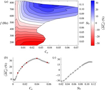
, calculated as an area-weighted and temporal average, is shown in figure 3(a) as a function of forcing amplitude and frequency. This response map can be loosely divided into pressure decrease and pressure recovery regimes by a horizontal line at
 $\mathit{St}_{{\it\theta}}\approx 0.07$
. Below this frequency, the base pressure reduction occurs due to strong shear layer amplification with a maximum at
 $\mathit{St}_{{\it\theta}}\approx 0.021$
(Zaman & Hussain Reference Zaman and Hussain1981). For the present experiment
 $D/{\it\theta}=92$
, so that turbulence may be regarded as ‘small’ compared to the large wake structure. This phenomenon is well understood, as discussed previously by Morrison & Qubain (Reference Morrison, Qubain and Eckhardt2009), Qubain (Reference Qubain2009) and Qubain & Morrison (Reference Qubain and Morrison2009): they also identified the novel pressure recovery regime, appearing here for forcing frequencies,
 $\mathit{St}_{{\it\theta}}\gtrsim 0.07$
, and amplitudes
 $C_{{\it\mu}}>0.005$
.
Effect of forcing amplitude and frequency on the mean base pressure coefficient. (a) Two-dimensional colour map, where contour levels denote 4.2 % intervals. (b) Effect of forcing amplitude at
 $\mathit{St}_{{\it\theta}}=0.107$
. Filled symbols denote values of
 $C_{{\it\mu}}$
used in figure 8(a). (c) Effect of forcing frequency at
 $C_{{\it\mu}}=0.018$
.

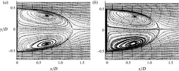
Mean velocity vectors and streamlines,
 $\mathit{Re}_{{\it\theta}}=1700$
at separation: (a) unforced, (b) forced,
 $\mathit{St}_{{\it\theta}}=0.076$
,
 $C_{{\it\mu}}\approx 0.03$
.

The relationship between blowing coefficient and change in base pressure coefficient at
 $\mathit{St}_{{\it\theta}}=0.107$
(the frequency at which maximum pressure recovery is observed) is illustrated in figure 3(b). There is a small initial reduction in base pressure at blowing coefficients below
 $C_{{\it\mu}}\approx 0.005$
, after which the pressure recovers rapidly. Above
 $C_{{\it\mu}}=0.01$
there is a gradual reduction in gradient, producing a broad region of pressure recovery with a maximum of 33 % at
 $C_{{\it\mu}}\approx 0.04$
. For constant amplitude forcing at
 $C_{{\it\mu}}=0.018$
, figure 3(c) shows that pressure recovery increases linearly up to
 $\mathit{St}_{{\it\theta}}\approx 0.1$
, where it saturates at
 $\langle \overline{{\rm\Delta}C_{p}}\rangle \sim 23\,\%$
. This suggests that the contours in the upper region of figure 3(a) may extend vertically to provide a wide frequency bandwidth over which pressure recovery can be obtained. This frequency plateau begins at
 $\mathit{St}_{{\it\theta}}\approx 0.1$
, that is, roughly five times the most amplified frequency of the shear layer instability.
Effect of forcing on mean velocity, with streamlines coloured by velocity magnitude: (a) unforced flow, (b) forced flow,
 $C_{{\it\mu}}=0.04$
,
 $\mathit{St}_{{\it\theta}}=0.107$
.

3.2. Mean velocity
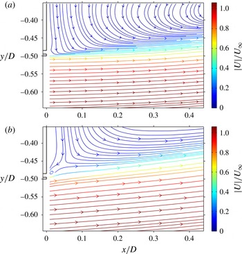
Figure 4 shows mean velocity vectors and streamlines calculated from preliminary PIV vector fields (Qubain Reference Qubain2009) that record the whole recirculation region. Here the vector spacing is 3.6 mm. In the unforced flow, the mean stagnation point occurs at an axial position,
 $x/D=1.27$
, while for the forced case, it is reduced slightly to
 $x/D=1.23$
. This is remarkable in that a drag reduction does not lead to an elongation of the recirculation region, even though the length of the recirculation bubble is shortened when forcing at lower frequencies,
 $\mathit{St}_{{\it\theta}}\approx 0.025$
, and the base pressure decreases. Figure 5 shows the detail close to separation (up to
 $x/D\approx 0.5$
) of streamlines and velocity magnitude in the separated shear layer for the unforced and forced case. With the improved resolution (vector spacing 0.2 mm), it appears that in the latter case there is a significant narrowing of the wake and an increase of velocity throughout the shear layer. Both the average length and width of the recirculation bubble are reduced. Interestingly, there is a reversal in the sign of streamline curvature immediately downstream of the trailing edge. This is characteristic of a local rise in pressure at the base, and adjacent to and slightly above the jet exit there is a small vortex. This is accompanied by a saddle point that forms the corner of the recirculation bubble. These data show that a base pressure rise is associated with a shortening of the bubble and narrowing of the wake due to the local change in the sign of streamline curvature near the trailing edge.
Premultiplied pressure spectra by azimuthal mode for the unforced and maximum pressure recovery cases: (a)
 $m=0$
, (b)
 $|m|=1$
, (c)
 $|m|=2$
. Black line, unforced; grey line, forced.

3.3. Base pressure fluctuations
Following the method of Rigas et al. (Reference Rigas, Oxlade, Morgans and Morrison2014b ), a Fourier decomposition of the pressure signal in the azimuthal direction gives spatial modes
 $$\begin{eqnarray}p_{m}(r,t)=\frac{1}{2{\rm\pi}}\int _{0}^{2{\rm\pi}}p(r,{\it\phi},t)\text{e}^{-\text{i}m{\it\phi}}\text{d}{\it\phi}.\end{eqnarray}$$
The spectral energy density of each mode
 ${\it\Phi}_{m}(r,\mathit{St})$
can be used to identify coherent structures in the wake, and when integrated provides the pressure variance per mode,
 $$\begin{eqnarray}\overline{p_{m}^{2}}(r)=\int _{0}^{\infty }\mathit{St}{\it\Phi}_{m}(r,\mathit{St})\text{d}(\log \mathit{St}).\end{eqnarray}$$
Owing to the limited frequency resolution of the static tappings, spectral analysis of the forced flow is performed on the transducer measurements, located at
 $r=0.3D$
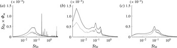
. Figure 6 compares the premultiplied spectral density for the unforced and forced flows, the latter at maximum pressure recovery,
 $C_{{\it\mu}}=0.04$
and
 $\mathit{St}_{{\it\theta}}=0.107$
. The unforced spectral density at this radius is qualitatively similar to the radially averaged result presented in figure 3 of Rigas et al. (Reference Rigas, Oxlade, Morgans and Morrison2014b
).
Within the pressure recovery regime, the effect of high-frequency forcing on pressure fluctuations is a broadband suppression occurring across all modes, without any obvious mode selection. This suggests a strong nonlinear coupling between the axisymmetric forcing and all the wake modes. Note that the marked reduction in the
 $|m|=1$
peak at
 $\mathit{St}_{D}\approx 0.2$
confirms that the forcing is able to attenuate the global instability or vortex shedding mode: we also observe a small shift in its frequency which increases with forcing amplitude for
 $C_{{\it\mu}}\gtrsim 0.005$
(see Oxlade Reference Oxlade2013).
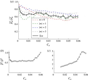
Figure 7(a) shows the mean-square pressure for each mode shape at a forcing frequency of
 $\mathit{St}_{{\it\theta}}=0.107$
and normalised by the mean-square pressure for the unforced case: it clearly decreases with increasing forcing amplitude. Comparison with figure 4(a) suggests an approximate correlation between the average pressure,
 $\langle \overline{{\rm\Delta}C_{p}}\rangle$
, and its variance up to
 $C_{{\it\mu}}\approx 0.04$
. However, at larger blowing coefficients, further reduction of mean-square pressure is not matched by an equivalent increase of mean pressure. Further insight is provided by figure 7(b,c), which shows the pressure variance of the vortex-shedding and shear layer modes respectively. The mean-square pressure associated with the vortex-shedding mode decreases initially for
 $C_{{\it\mu}}\lesssim 0.005$
, then remains constant until the maximum pressure recovery at
 $C_{{\it\mu}}\approx 0.04$
, after which there is a sharp increase: for larger forcing amplitudes (not shown) this mode is strongly amplified. The mean-square pressure associated with the shear layer mode (measured by a single outer transducer at
 $r/D=0.44$
) exhibits a sharp increase just after the optimum forcing amplitude. These data suggest that, above
 $C_{{\it\mu}}\approx 0.04$
, the wake modes are amplified by the forcing: in this sense, the natural wake modes compete with the pressure recovery mechanism by increasing entrainment when
 $C_{{\it\mu}}\gtrsim 0.04$
. This explains why the pressure fluctuations continue to decrease at larger forcing amplitudes even though the mean pressure recovery is lost.
Effect of forcing amplitude on mean-square base pressure for
 $\mathit{St}_{{\it\theta}}=0.107$
, by (a) azimuthal mode shape, (b) vortex shedding mode, and (c) shear layer mode.

3.4. Jet structure
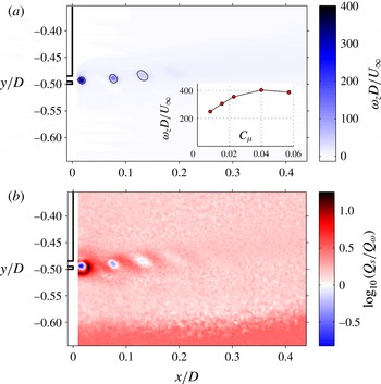
An explanation of this phenomenon is provided in figure 8: the jet produces strong and distinct vortex rings that advect within the shear layer and remain coherent for approximately
 $x/D<0.2$
. Measured over the adjacent vortex positions in figure 8(a), their advection velocity is roughly proportional to
 $C_{{\it\mu}}$
and equal to
 $0.57U_{\infty }$
. They have an initial diameter approximately equal to the jet orifice width. While the vorticity of the primary vortex is about 50 times the mean vorticity of the separating boundary layer, its circulation is only about 10 % of the mean boundary layer circulation. It is expected that the jet efflux produces a pair of counter-rotating, concentric vortex rings, the outer one with vorticity of opposite sign to that of the boundary layer. Their cancellation leaves the inner vortex ring with vorticity of the same sign as that of the boundary layer.
Phase-locked quantities for the maximum pressure recovery (
 $C_{{\it\mu}}=0.04$
,
 $\mathit{St}_{{\it\theta}}=0.107$
). (a) Planar vorticity,
 ${\it\omega}_{z}D/U_{\infty }$
, with vortices identified by a single contour of swirl strength,
 ${\it\lambda}_{i}=10$
. The inset shows the peak vorticity
 ${\it\omega}_{z}$
of the initial vortex as a function of
 $C_{{\it\mu}}$
, corresponding to conditions in figure 3(b) denoted by filled symbols. (b) Corresponding
 $Q_{s}/Q_{{\it\omega}}$
.

The magnitude of the pressure recovery is strongly dependent on the strength of the vortex produced by the jet. Figure 8(a) (inset) shows the maximum vorticity of the jet vortex,
 ${\it\omega}_{z}D/U_{\infty }$
, as a function of
 $C_{{\it\mu}}$
at
 $\mathit{St}_{{\it\theta}}=0.107$
. The initial increase in forcing amplitude strengthens the primary vortex up to
 $C_{{\it\mu}}\approx 0.04$
, where it reaches saturation: inspection of figure 4(b) shows that the maximum pressure recovery coincides with maximum vortex strength. At forcing amplitudes
 $C_{{\it\mu}}\gtrsim 0.04$
, the jet vortex is observed to break down immediately into two or more vortical structures (Oxlade Reference Oxlade2013). This causes the increased amplification of the wake modes (figure 7
b,c), and consequently the reduction in pressure recovery.
An important feature of the jet flow topology is highlighted in figure 8(b), which compares the ratio of
 $Q_{s}$
and
 $Q_{w}$
, respectively, the strain and rotational components of the second invariant,
 $Q$
, of the strain rate tensor,
 $\unicode[STIX]{x1D634}_{ij}$
:
 $$\begin{eqnarray}Q=Q_{s}+Q_{{\it\omega}}=-{\textstyle \frac{1}{2}}\unicode[STIX]{x1D634}_{ij}\unicode[STIX]{x1D634}_{ji}+{\textstyle \frac{1}{4}}{\it\omega}_{i}{\it\omega}_{i},\end{eqnarray}$$
where in the (
 $x,y$
)-plane,
 $$\begin{eqnarray}\unicode[STIX]{x1D634}_{xy}^{2}=\left(\frac{\partial u}{\partial x}\right)^{2}+\frac{1}{2}\left(\frac{\partial u}{\partial y}+\frac{\partial v}{\partial x}\right)^{2}+\left(\frac{\partial v}{\partial y}\right)^{2}\end{eqnarray}$$
and
 $$\begin{eqnarray}\frac{1}{2}{\it\omega}_{z}^{2}=\frac{1}{2}\left(\frac{\partial u}{\partial y}-\frac{\partial v}{\partial x}\right)^{2}.\end{eqnarray}$$
In general, the left-hand side of (3.3) is the small difference between two large quantities because shear layer turbulence consists predominantly of vortex sheets or internal shear layers which have nearly opposite
 $\unicode[STIX]{x1D634}_{ij}$
and
 ${\it\omega}_{i}$
and, being approximately plane with nearly straight streamlines, do not contribute significantly to the pressure. This is not the case in figure 8(b): where
 $Q_{s}/Q_{{\it\omega}}\gg 1$
,
 $Q\approx Q_{s}$
and the local flow is predominantly a straining motion with strong dissipation. Alternatively, where
 $Q_{s}/Q_{{\it\omega}}\ll 1$
,
 $Q\approx Q_{{\it\omega}}$
and the local flow is dominated by strongly rotating but weakly dissipative motion. Figure 8(b) shows that the distinction between these two topologies is unambiguous since the jet structure comprises strongly rotational vortex cores immediately surrounded by, and joined by, regions of nearly pure shear. Consequently, in regions where the flow is dominated by these structures, the sign of
 $Q$
is sufficient to distinguish between rotation and shear.
3.5. The pressure recovery mechanism
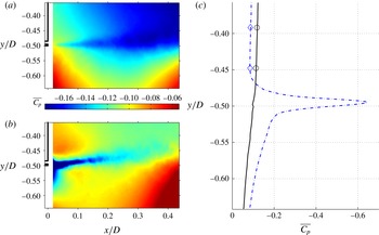
The static pressure field for the unforced and forced flows is compared in figure 9. In the forced case the jet creates a thin region of very low pressure, the minimum of which is coincident with the trajectory of the jet vortex cores. The resulting pressure recovery is clearly visible throughout the flow field, encompassing both the base region and the outer side of the shear layer for
 $x/D>0.3$
. Figure 9(b) shows that the computed pressure distribution is in close agreement with the transducer measurements on the base of the body.
Time-averaged pressure coefficient,
 $\overline{C_{p}}$
, obtained as the integral of the velocity field in the
 $(x,y)$
-plane: colour scale limits for the forced flow are truncated to match the limits of the unforced flow. (a,b) Pressure maps, (a) unforced and (b) forced,
 $\mathit{St}_{{\it\theta}}=0.107$
,
 $C_{{\it\mu}}=0.04$
; note the minimum
 $\overline{C_{p}}\approx -0.6$
. (c) Corresponding line graphs for
 $x/D=0.0$
: ——, unforced; –
 $\cdot$
–
 $\cdot$
–, forced. Symbols denote the corresponding base pressure transducer measurements.

Bradshaw & Koh (Reference Bradshaw and Koh1981) have shown that the Poisson equation for pressure fluctuations may be written as
 $$\begin{eqnarray}-\!\frac{{\rm\nabla}^{2}p}{{\it\rho}}=-2Q=\unicode[STIX]{x1D634}_{ij}\unicode[STIX]{x1D634}_{ji}-\frac{1}{2}{\it\omega}_{i}{\it\omega}_{i},\end{eqnarray}$$
where the right-hand side is decomposed into the sum of symmetric (straining) and antisymmetric (rotational) components of the strain rate tensor. Although this decomposition is not unique (Adrian Reference Adrian1982), the former may be taken to represent the non-local generation of pressure by stagnation points in the instantaneous streamline pattern (‘eddy collisions’) while the rotational term (enstrophy) indicates local regions of low pressure created by centripetal acceleration.
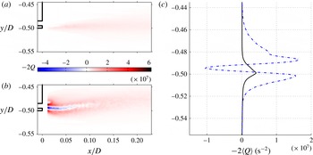
Figure 10 compares the distribution of time-averaged
 $-2Q$
((3.6) in the (
 $x,y$
)-plane) for the unforced and forced flow at maximum pressure recovery. The vertical profiles (figure 10
b) show
 $-2\langle Q\rangle$
, the second invariant averaged over a short streamwise region near the jet. This clearly shows that the forced wake is dominated by a narrow region of large enstrophy (
 $2\langle Q\rangle \gg 0$
) bounded on each side by a strong shear layer (
 $2\langle Q\rangle \ll 0$
), associated with high dissipation and responsible for a reduction in entrainment. Specifically, the term
 $\overline{(\partial u/\partial y)(\partial v/\partial x)}$
determines the sign of
 $Q$
and therefore whether a region is one of large, nearly irrotational dissipation or one of large enstrophy.
Comparison of the second invariant,
 $-2Q$
, in the forced and unforced flows. (a,b) Time-averaged colour maps, (a)
 $C_{{\it\mu}}=0.04$
and (b) unforced. (c) Vertical profiles of
 $-\langle 2Q\rangle$
averaged for
 $0.01<x/D<0.07$
: ——, unforced; –
 $\cdot$
–
 $\cdot$
–, forced.

4. Discussion and conclusions
The effect of pressure recovery behind a bluff body with a sharp trailing edge is generic in that we have also been able to demonstrate it for turbulent separation from a bluff body of rectangular cross-section (Cabitza Reference Cabitza2013) as well as that from a backward-facing step (Qubain Reference Qubain2007). The unifying feature of these experiments is that the entrainment and therefore the growth rates of these wakes have been reduced, with a concomitant reduction in pressure drag. The mechanism by which pressure is recovered in the wake appears to be the creation of a narrow region of strong enstrophy bounded on each side by a very strong shear layer: the region of large enstrophy is coincident with the vortex core trajectory, and since each vortex is instantaneously demarcated by a region of very strong shear, its advection results in a time-averaged shear layer on each side. These are associated with high dissipation and responsible for the reduction in entrainment and hence drag on the body.
These effects appear to induce large scale changes in the wake, where the length of the recirculation region is slightly reduced by high-frequency forcing. Near the base of the body, there is a point of inflection in the separating streamline which leads to a narrowing of the wake. It seems likely that the models proposed by Gerrard (Reference Gerrard1966) and Roshko (Reference Roshko1993) would require modification in order to describe this effect. Further studies are underway involving the simultaneous measurement of base pressure and the vorticity field.
Acknowledgements
We are indebted to Ferrari S.p.A. and to EPSRC (grant number EP/I005684) for financial support.