

1. INTRODUCTION
From the special theory of relativity we know that the shock wave velocity is bounded by the speed of light, c. The theoretical foundation of relativistic shock waves is based on relativistic hydrodynamics (Landau & Lifshitz, Reference Landau and Lifshitz1987) and was first analyzed by Taub (Reference Taub1948). Relativistic shock waves may be of importance in intense stellar explosions or in collisions of extremely high energy nuclear particles. Furthermore, relativistic shock waves may be a new route for fast ignition nuclear fusion (Eliezer & Martinez Val, Reference Eliezer and Martinez Val2011; Eliezer, Reference Eliezer2012).
The highest laser-induced pressures, on the order of 1 Gbar, have been obtained during the collision of a target with an accelerating foil. This acceleration was achieved by the ablation of laser produced plasma or by X-rays created by laser plasma interaction. The foil absorbs the laser energy, plasma is then obtained, and the foil is accelerated like a rocket (Eliezer, Reference Eliezer2002). In this way, the flyer stores kinetic energy from the laser during the acceleration period and delivers it during the collision with a target, in the form of thermal energy. The laser driven flyer can achieve much higher pressures on impact than the shock wave pressure obtained directly by the laser ablation. In 1994 at the Lawrence Livermore National Laboratory (USA), a pressure of about 1 Gbar was created by accelerating a foil with soft X-rays from the indirect drive (Cauble et al., Reference Cauble, Phillion, Hoover, Holmes, Kilkenny and Lee1993). Planar foil targets were accelerated to 1000 km/s at the Institute of Laser Engineering at the Osaka University in Japan (Azechi et al., Reference Azechi, Sakaiya, Watari and Karasik2009). The targets were about 20 microns thick and were made of polystyrene doped with 0.4% (atomic) bromine. The acceleration driver was a 0.35 µm wavelength laser with energy of 1.5 kJ, 2 ns pulse width and an irradiation of 4 × 10¹⁴ W/cm2.
For I L < 1016 W/cm2, the ablation pressure is dominant. For this regime of laser irradiances, the shock wave fast ignition scheme was suggested using appropriate flyers (Eliezer & Martinez Val, Reference Eliezer and Martinez Val2011; Murakami et al., Reference Murakami, Nagatomo, Azechi, Ogando, Perlado and Eliezer2006). The ignition is achieved by launching a shock wave during the final stages of the implosion. For I L ≫ 1016 W/cm2, the radiation pressure is the dominant pressure at the solid-vacuum interface and the ablation pressure is negligible. In this paper, it is suggested that for very high laser irradiance, the ponderomotive force can accelerate a micro-foil to relativistic velocities.
Ultrahigh accelerations on the order of 1020 cm/s2 were predicted for high density plasma blocks created in sub-picosecond laser pulses with more than terawatt intensity. This effect was obtained by using two fluid simulations for laser plasma interaction where the nonlinear ponderomotive force was dominant (Hora, Reference Hora2012; Lalousis et al., Reference Lalousis, Földes and Hora2012). Ion acceleration by ponderomotive force to relativistic velocities was also obtained using particles in cell simulations (Esirkepov et al., Reference Esirkepov, Borghesi, Bulanov, Mourou and Tajima2004; Robinson et al., Reference Robinson, Zepf, Kar, Evans and Bellei2008). This acceleration is similar to the old proposal to accelerate space ships to relativistic velocities by laser pressure radiation (Marx, Reference Marx1966; Redding, Reference Redding1967; Simmons & McInnes, Reference Simmons and McInnes1993). Ion acceleration in thin films driven by laser pressure in the domain of 1018 W/cm2 was reported (Maksimchuk et al., Reference Maksimchuk, Gu, Flippo, Umstadter and Bychenkov2000).
In this paper, it is suggested that state of the art and future high power lasers will enable to accelerate micro-foils to relativistic velocities. The novel aspects of the impact of this accelerated foil with a target or two colliding accelerating foils in the laboratory is analytically calculated and numerically presented.
In Section 2, we describe the relativistic shock waves formalism and give explicit Hugoniot relations for extreme relativistic and ideal gas equations of state (EOS). In Section 3, we calculate the impact of a relativistic foil with a target. The hydrodynamic and thermodynamic variables, such as shock velocity, flow velocity, compression, pressure, temperature, and internal energy are obtained. In Section 4, we describe a scenario of accelerating a micro-foil by using the state of the art and future high power lasers. A short discussion is presented in the last section of this paper.
2. RELATIVISTIC SHOCK WAVES
Relativistic shock waves are considered in the context of relativistic fluid dynamics (Landau & Lifshitz, Reference Landau and Lifshitz1987). The equations of motion are described by the relativistic energy-momentum four-tensor T μν given by
 $$T_{{\rm \mu} {\rm \nu}} = \lpar e + P\rpar U_{{\rm \mu}} U_{{\rm \nu}} + Pg_{{\rm \mu} {\rm \nu}}.$$
A Greek index takes the values: 0, 1, 2, 3 while we use the Latin index for the space values 1, 2, 3. U μ = (γc, γv 1, γv 2, γv 3) is the four-velocity where (v 1, v 2, v 3) is the fluid element velocity in three dimension (x, y, z), e is the internal energy density of the fluid which includes the rest energy mass of the fluid particles, P is the pressure, the metric tensor g μν is g 00 = −1, g 11 = g 22 = g 33 = 1, g μν = 0 for μ ≠ ν and for a three dimension velocity v one defines
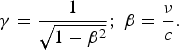 $${\rm \gamma} = {1 \over \sqrt{1 - {\rm \beta}^2}}\semicolon \; {\rm \beta} = {{\rm \nu} \over c}.$$
The equations describing the relativistic fluid motion (neglecting internal friction and thermal conduction) are
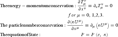 $$\eqalign{& {\rm Theenergy - momentumconservation}:\displaystyle{{\partial T_\mu ^\nu } \over {\partial x^v }} \equiv \partial _v T_\mu ^v = 0\, \cr & \quad \quad \quad \quad \quad \quad \quad \quad \quad \quad \quad \quad \quad \quad for\,\mu = 0{\rm , }\>1{\rm , }2{\rm , }3. \cr & {\rm The}\;{\rm particle number conservation}:\displaystyle{{\partial (nU^\mu {\rm )}} \over {\partial x^\mu }} \equiv \partial _\mu \left( {nU^\mu } \right) = 0 \cr & {\rm The equation of State}:\quad \quad \quad \quad \quad \quad \quad \quad P = P\left( {e{\rm ,}\>\;n} \right)}$$
The Einstein summation convention (from 0 to 3) is assumed for identical indexes. Since Eq. (1) is the starting point of our calculation we write it more explicitly
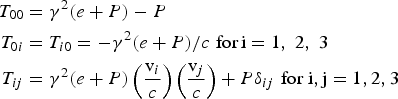 $$\eqalign{T_{00} &= {\rm \gamma}^2 \lpar e + P\rpar - P \cr T_{0i} &= T_{i0} = - {\rm \gamma}^2 \lpar e + P\rpar / c\, \,\hbox{for}\, \hbox{i} = 1\comma \; 2\comma \; 3 \cr T_{ij} &= {\rm \gamma}^2 \lpar e + P\rpar \left({\hbox{v}_i \over c} \right) \left({\hbox{v}_j \over c} \right) + P {\rm \delta}_{ij}\, \,\hbox{for i}, \hbox{j} = 1, 2, 3}$$
δij = 1 for i = j and δij = 0 for i ≠ j. T 00 is the energy density [J/m3], −T 0i/c is the momentum component density [kg/m2 × s] and T ij is the momentum flux density.
We assume a one-dimensional (1D) shock wave where the shock propagates in the x direction and the shock wave surface singularity is in the y-z plane. Furthermore, the shock wave is time independent by looking into a coordinate system where the shock front is at rest. In this shock wave reference system (the shock system), the observer is at rest relative to the material on both sides of the shock front. We use the subscript 0 and 1 to denote the variables in front (where the shock wave did not arrive yet) and in the back (the shocked area) of the shock wave, respectively. The physical quantities: pressure P, particle density n, mass density ρ, energy density e, entropy density s, and temperature T are measured in their proper frame of reference, defined as the reference frame where the corresponding fluid element is at rest. The flow velocities v 0 and v 1, assumed in the x direction, are measured in the shock wave reference system. In this case, we define β0 = v 0/c, β1 = v 1/c, and γ0, γ1 according to Eq. (2).
The conservation laws across the shock wave singularity describe the flux densities conservation of energy −c[T 0x]0 = −c[T 0x]1 and momentum [T xx]0 = [T xx ]1 as defined in Eq. (4) and the particle number flux defined by [nU x]0 = [nU x]1. These conservation laws are explicitly given by the following equations accordingly
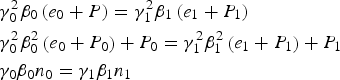 $$\eqalign{&{\rm \gamma}_0^2 {\rm \beta}_0 \left(e_0 + P \right)= {\rm \gamma}_1^2 {\rm \beta}_1 \left(e_1 + P_1 \right)\cr &{\rm \gamma}_0^2 {\rm \beta}_0^2 \left(e_0 + P_0 \right)+ P_0 = {\rm \gamma}_1^2 {\rm \beta}_1^2 \left(e_1 + P_1 \right)+ P_1 \cr &{\rm \gamma}_0 {\rm \beta}_0 n_0 = {\rm \gamma}_1 {\rm \beta}_1 n_1}$$
Regarding the particle conservation, the third of Eq. (5), it is important to clarify that for very high temperature T new particles can be created, such as electron-positron pairs. In this case, we consider the electric charge conservation (of the electron-positron system in this example).
The solution of Eq. (5) yields
 $$\eqalign{{\hbox{v}_0 \over c} ={\rm \beta}_0 =\sqrt{{\lpar P_1 - P_0\rpar \lpar e_1 + P_0\rpar \over \lpar e_1 - e_0\rpar \lpar e_0 + P_1\rpar }} \cr {\hbox{v}_1 \over c}= {\rm \beta}_1 =\sqrt{{\lpar P_1 - P_0\rpar \lpar e_0 + P_1\rpar \over \lpar e_1 - e_0\rpar \lpar e_1 + P_0\rpar }}.}$$
The relative velocity between the flows v 0 and v 1 on both sides of the singularity is given by v 01
 $${\hbox{v}_{01} \over c}= {\rm \beta}_{01} = {{\rm \beta}_0 - {\rm \beta}_1 \over 1 - {\rm \beta}_0 {\rm \beta}_1} = \sqrt{{\lpar P_1 - P_0\rpar \lpar e_1 - e_0\rpar \over \lpar e_0 + P_1\rpar \lpar e_1 + P_0\rpar }}.$$
Substituting v0 and v1 into the third of Eq. (5) one gets the Hugoniot relation (Landau & Lifshitz, Reference Landau and Lifshitz1987; Taub, Reference Taub1948), first derived by Taub (Reference Taub1948),
 $${\lpar e_1 + P_1\rpar ^2 \over n_1^2} - {\lpar e_0 + P_0\rpar ^2 \over n_0^2} = \lpar P_1 - P_0\rpar \left[{\lpar e_0 + P_0\rpar \over n_0^2} + {\lpar e_1 + P_1\rpar \over n_1^2} \right].$$
Before proceeding with the relativistic calculations it is useful to check the non-relativistic (NR) limit of Eqs. (4), (5), and (8). The NR limit is defined by v ≪ c. The relativistic internal energy e [J/m3] includes the rest energy nmc 2 = ρc 2 of the fluid particles, where m is the rest mass of one particle. In going to the NR limit, one has to take into account the fluid motion and therefore before doing the limit properly one has to substitute ρ by ρ/γ = ρ(1 − v2/c 2)1/2 ≈ ρ[1 − v2/(2c 2)]. One can define the internal energy per unit mass E(J/kg) by the relation e = ρc 2 + ρE, so that the NR limit of e is ρc 2 + ρE − (1/2)ρv2. Thus, the non-relativistic energy-momentum four-tensor T μν is given by: T 00 → ρc 2 + ρE+ (1/2)ρv2, −cT i0 → ρc 2vi + [ρE + P + (1/2)ρv2]vi, T ij → ρvivj + Pδij. Furthermore, taking into account that in the NR limit P and ρE are much smaller than ρc 2 then Eqs. (5) go to the standard Hugoniot equations in the shock wave frame of reference: Energy conservation, {[ρE + P + (1/2)ρv2]v}0 = {[ρE + P + (1/2)ρv2]v}1; momentum conservation, {P + ρv2}0 = {P + ρv2}1 and mass conservation, {ρv}0 = {ρv}1. Similarly, the Hugoniot Eq. (8) goes to its NR limit: E 1 − E 0 = (1/2)(P 0 + P 1)(1/ρ0 − 1/ρ1).
In order to solve the equations of motion, the knowledge of the EOS is required. We consider in this paper two EOS: The extreme relativistic (ER) EOS
 $$P = {1 \over 3} e\comma \;$$
and the ideal gas (IG) EOS
 $$\eqalign{e &= {\rm \rho} c^2 + {P \over \Gamma - 1} \cr P &= nk_B T}\comma \;$$
Γ is the specific heat ratio and k B is the Boltzmann constant. The relativistic Hugoniot lines obtained from Eq. (8) for P 0 = 0 and the EOS of Eqs. (9) and (10) are
 $$\eqalign{&ER - EQS\, \hbox{Hugoniot\colon } \displaystyle{{P_1 \over {\rm \rho}_0 c^2} = {1 \over 12}} \left[\matrix{\displaystyle\left({{\rm \rho}_1 \over {\rm \rho}_0} \right)^2 + \left({{\rm \rho}_1 \over {\rm \rho}_0} \right) \sqrt{\left({{\rm \rho}_1\over {\rm \rho}_0} \right)^2 + 48} } \right]\cr &IG - EOS\, \hbox{Hugoniot\colon } \left\{\matrix{\displaystyle{{P_1 \over {\rm \rho}_0 c^2}} = \left({\lpar \Gamma - 1\rpar ^2 \over \Gamma} \right)\left({{\rm \rho}_1 \over {\rm \rho}_0} \right)^2 - \left({\Gamma^2 - 1 \over \Gamma} \right)\left({{\rm \rho}_1 \over {\rm \rho}_0} \right) \cr \displaystyle{{k_B T_1 \over mc^2}} = \left({\lpar \Gamma - 1\rpar ^2 \over \Gamma} \right)\left({{\rm \rho}_1 \over {\rm \rho}_0} \right)- \left({\Gamma^2 - 1 \over \Gamma} \right)} \right.}$$
Note that for the ideal gas EOS our relativistic approach in Eq. (11) starts from a compression of (Γ + 1)/(Γ − 1), namely for Γ = 5/3 we have ρ1/ρ0 = 4, P 1 = 0, T 1 = 0 and the relativistic Hugoniot is for ρ1/ρ0 > 4. However, for the general case we cannot assume P 0 = 0 and in this case we have
 $$\eqalign{&{\rm \kappa} \equiv {{\rm \rho}_1 \over {\rm \rho}_0}\semicolon \; {\rm \kappa}_0 \equiv {\Gamma + 1 \over \Gamma - 1}\semicolon \; \Pi_i \equiv {P_i \over {\rm \rho}_0 c^2}\, \,\hbox{for}\, \hbox{i} = 0\comma \; 1\semicolon \; \cr &\Pi_1^2 + b\Pi_1 + c = 0\cr \Pi_1 &= \left({1 \over 2} \right)\left(-b + \sqrt{b^2 - 4c} \right)\cr b &= {\left(\Gamma - 1 \right)^2 \over \Gamma} \left({\rm \kappa}_0 {\rm \kappa} - {\rm \kappa}^2 \right)+ \Pi_0 \left(\Gamma - 1 \right)\left(1 - {\rm \kappa}^2 \right)\cr c &= {\left(\Gamma - 1 \right)^2 \over \Gamma} \left({\rm \kappa} - {\rm \kappa}_0 {\rm \kappa}^2 \right)\Pi_0 - {\rm \kappa}^2 \Pi_0^2}$$
For Π0 = 0 we get Eq. (11) for the ideal gas EOS. However, for a nonzero Π0 we have two solutions but only the plus sign is appropriate in Eq. (12) since c < 0 and Π1 > 0. Note also that Π1 = 0 only if Π0 = 0 and κ = 1 for Π1 = Π0 as physically requested. In general, Π1 is a function of κ with Π0 as a parameter, Π1 = f(κ;Π0) and Π1 is positive for compressions larger than 1 as requested by a shock wave.
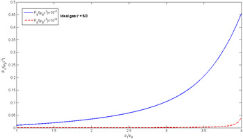
The relativistic Hugoniot of the (dimensionless) pressure P1/(ρ0c 2) is plotted in Figure 1 in the domain 1 < ρ1/ρ0 < 4 for initial pressures P 0/(ρ0c 2) = 10−2 and 10−4 using an ideal gas EOS with Γ = 5/3. One can see that for initial low pressures that we are interested in this paper, P 0/(ρ0c 2) ≪ 10−4, the Hugoniot domain of interest is for ρ1/ρ0 > 4.
Hugoniot of the (dimensionless) pressure P 1/(ρ0c 2) in the domain 1 < ρ1/ρ0 < 4 for initial pressures P 0/(ρ0c 2) = 10−2 and 10−4 using an ideal gas EOS with Γ = 5/3.

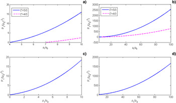
These Hugoniot lines for the dimensionless pressure P 1/(ρ0c 2) of Eq. (11) are plotted in Figure 2. The calculations were done in the relativistic approximation for the ideal gas EOS with Γ = 5/3 and 4/3. In Figure 1a, the compression up to 10 and in 1b compression up to 100 are plotted. The Hugoniot curves for the extreme relativistic EOS are shown for compression up to 10 in 1c and up to 100 in Figure 1d.
Hugoniot lines for the dimensionless pressure P1/(ρ0c2). The Hugoniot curves for the ideal gas EOS with Γ = 5/3 and 4/3 are shown in (a) for compression up to 10 and in (b) for compression up to 100. The Hugoniot curves for the extreme relativistic EOS are shown for compression up to 10 in (c) and up to 100 in (d).

3. COLLISION BETWEEN A FLYER AND A TARGET
The highest laser induced pressures, on the order of 109 bars, have been obtained during the collision of a target with an accelerating foil. This acceleration was achieved by laser produced plasma or by X-rays from a cavity produced by laser plasma interactions. In this section, we solve this relativistic collision problem for a symmetrical collision, namely the target and the flyer have the same material properties (e.g., an aluminum-aluminum collision). In the relativistic collision, we derive pressures higher by many orders of magnitude than presently obtained.
The flyer has a known initial (before impact) velocity u f in the laboratory frame of reference. This velocity is calculated theoretically in the next section and it seems possible to measure it experimentally using the relativistic Doppler effect (DE).
 $$\eqalign{longitudinal \;DE\colon {{\rm \lambda}_0 \over {\rm \lambda}_s} &= {{\rm \nu}_s \over {\rm \nu}_0} = \sqrt{{1 + {\rm \beta}_f \over 1 - {\rm \beta}_f}}\semicolon \; {\rm \beta}_f = {u_f \over c} \cr transversal \;DE\colon {{\rm \nu}_s \over {\rm \nu}_0} &= {\rm \gamma}_f \lpar 1 + {\rm \beta}_f \cos {\rm \theta}_o\rpar \semicolon \; {\rm \gamma}_f {1 \over \sqrt{1 - {\rm \beta}_f^2}}.}$$
The subscripts s and o refer to observer and source frames of reference accordingly, θo is the angle between the flyer motions and the observer, λ and ν are the appropriate wavelength and frequency of the electromagnetic wave. It is interesting and might be experimentally useful to see the νs/νo (θo = π/2) = γf relativistic effect.
We chose for simplicity the accelerated micro-foil (the flyer) and the target to be of the same material. After the collision a shock wave S1 will move into the target and another shock wave S2 will move into the flyer. The proper fluid quantities: density ρ = mn, where m is the mass of fluid particles and n the particle density, the pressure P, the energy density e, and temperature T before collision are denoted by subscript zero and after collision by subscript 1.
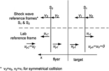
In Figure 3, a schematic description of the two shock waves is given with the appropriate notations in the laboratory frame of reference and in the two shock waves frame of reference S1 and S2. We denote by u the different velocities in the laboratory frame and by v the appropriate velocities in the S1 and S2 where the shock wave 1 and 2 are accordingly at rest. For the symmetrical collision we have v 3 = v 0 and v 2 = v 1.
Flow (u p0, u p1, u p2) and shock waves (u s1, u s2) velocities after impact of flyer and target in the laboratory frame of reference. The flow velocities (v 0, v1,v 2 = v 1,v 3 = v 0) are also defined in the shock wave reference frames S1 and S2.

If the 0 domain of the target is at rest in the laboratory then in this frame of reference the shock velocity u s = −v0. Note that v0 > 0 and u s < 0 means that the positive x coordinate is defined toward the back of the shock wave. Using Eqs. (6) with the previous definitions, β0 = v0/c, β1 = v1/c, and βf = u f/c where u f is the flyer velocity in the laboratory frame of reference while v0 and v1 are the flow velocities in the shock wave frames of reference S1 and S2, we get the shock waves velocities in the laboratory frame of reference
 $$\eqalign{{u_{s1} \over c} &= -{\rm \beta}_0 = - \sqrt{{\left(P_1 - P_0\right)\left(e_1 + P_0\right)\over \left(e_1 - e_0\right)\left(e_0 + P_1 \right)}} \cr {u_{s2} \over c} &= {{\rm \beta}_1 + {\rm \beta}_f \over 1 + {\rm \beta}_1 {\rm \beta}_f} = {1 + {\rm \beta}_f \sqrt{\displaystyle{\left(e_1 - e_0\right)\left(e_1 + P_0 \right)\over \left(P_1 - P_0\right)\left(e_0 + P_1\right)}} \over {\rm \beta}_f + \sqrt{\displaystyle{\left(e_1 - e_0 \right)\left(e_1 + P_0 \right)\over \left(P_1 - P_0 \right)\left(e_0 + P_1 \right)}}}.}$$
In the second relation of Eq. (14), the appropriate relativistic addition of velocities was used.
In the non-relativistic case, the Galilean transformations yield for the particle velocity in the laboratory frame u p1 = −(v1 − v0) at the SW1 surface singularity and u p1 = (v1 − v0) − u f at the SW2 surface singularity. From these two equations we get the well-known result: u f = 2u p1. We use now the same procedure by using the relativistic Lorentz transformation.
From Eq. (7) we get at the S1 surface singularity the particle flow velocity u p1 in the shocked area in the laboratory frame of reference
 $$u_{\,p1} = \hbox{v}_{01} = -c \sqrt{{\left(P_1 - P_0\right)\left(e_1 - e_0 \right)\over \left(e_0 + P_1 \right)\left(e_1 + P_0 \right)}}$$
On the other hand, at the S2 surface singularity, the particle flow velocity u p1 in the shocked area in the laboratory frame of reference is
 $$u_{\,p1} = {\hbox{v}_{01} - u_f \over 1 - \hbox{v}_{01} u_f /c^2}.$$
Using Eqs. (15) and (16) we get the relation
 $$\sqrt{{\left(P_1 - P_0 \right)\left(e_1 - e_0 \right)\over \left(e_0 + P_1 \right)\left(e_1 + P_0 \right)}} = {1 - \sqrt{1 - {\rm \beta}_f^2} \over {\rm \beta}_f}$$
These relations yield the known result u f = 2u p1 in the non relativistic limit.
The above analysis for the collision between a flyer and a target yields three equations: the Hugoniot Eq. (8), the impact relation given by Eq. (17), and the equation of state P = P(e, n). Therefore, we have three equations with three unknowns: e 1, P 1, and n 1 assuming that we know the initial conditions e 0, P 0, and n o and we measure experimentally the flyer impact velocity u f. We shall solve these equations using the EOS of extreme relativistic and ideal gas as given by Eqs. (9) and (10), namely we calculate e 1, P 1, and ρ1 as a function of u f. The initial conditions for our suggested impact are: P 0, e 0 = ρ0c 2 + P 0/(Γ − 1) for an initial density ρ0. However, since in the impact under consideration the initial pressure is extremely small (on the relativistic scale) we can take P 0 = 0 according to Eqs. (12) as described in Figure 1.
For the extreme relativistic EOS, the solution of the Hugoniot Eq. (8) and the EOS Eq. (9) gave our first relation of Eq. (11). The solution of this equation with the impact Eq. (17) yields the following solution
 $$\eqalign{&{P_1 \over {\rm \rho}_0 c^2} = {1 - {\rm \beta}_f^2 / 3 - \sqrt{1 - {\rm \beta}_f^2} \over -1 + {\rm \beta}_f^2 + \sqrt{1 - {\rm \beta}_f^2}} \cr &{{\rm \rho}_1 \over {\rm \rho}_0} = {P_1 \over {\rm \rho}_0 c^2} \sqrt{{6 \over 2 + \displaystyle{P_1 \over {\rm \rho}_0 c^2}}} \cr &\left({e_1 \over {\rm \rho}_0 c^2} \right)= 3 \left({P_1 \over {\rm \rho}_0 c^2} \right)}$$
For the ideal gas EOS, the solution of the Hugoniot Eq. (8) and the EOS Eq. (10) gave our second relation of Eq. (11). This equation with the impact Eq. (17) yields the following equation
 $$\eqalign{&{\left(\Gamma - 1 \right)\left[\left({{\rm \rho}_1 \over {\rm \rho}_0} \right)-1 \right]\left({P_1 \over {\rm \rho}_0 c^2} \right)+ \left({P_1 \over {\rm \rho}_0 c^2} \right)^2 \over \left[\left({P_1 \over {\rm \rho}_0 c^2} \right)+ 1 \right]\left[\left(\Gamma - 1 \right)\left({{\rm \rho}_1 \over {\rm \rho}_0} \right)+ \left({P_1 \over {\rm \rho}_0 c^2} \right)\right]} = B \cr &B \equiv {2 - {\rm \beta}_f^2 - 2 \sqrt{1 - {\rm \beta}_f^2} \over {\rm \beta}_f^2}}$$
B = 0 for βf = 0, B = 1 for βf = 1, and B(βf) is a monotonic increasing function of βf. Solving Eqs. (19) and the Hugoniot for the ideal gas (second relation of Eq. (11)) we get the following compression as a function of B(βf) and Γ:
 $${{\rm \rho}_1 \over {\rm \rho}_0} = {\left(1 - B\right)\pm \Gamma \sqrt{1 - B} \over \left(1 - B \right)\left(\Gamma - 1 \right)}.$$
One can directly check that this solution satisfies Eqs. (19) and the second relation of Eq. (11). B is defined in the second Eq. (19), so that the compression as a function of the flyer velocity βf is obtained. Substituting the compression from Eq. (20) into Eqs. (10) and (11) for the ideal gas EOS one gets the pressure, the temperature, and the internal energy for the shocked impact target. Since B < 1 and Γ > 1 and the compression is positive only for the solution with + sign in Eq. (20) is physical.
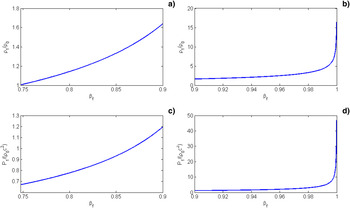
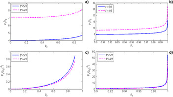
Numerical solutions for the density and pressure of the shocked impact target are given in Figures 4 and 5 for the extreme relativistic and ideal gas equations of states accordingly. Figure 4 shows the density and pressure of the shocked impact target as a function of the foil velocity βf for extreme relativistic equation of states. The compression is shown Figure 4a for velocities from about 0.75c up to 0.9c and in Figure 4b for velocities from 0.9c to 0.999c. The pressure is shown Figure 4c for velocities from about 0.75c up to 0.9c, and in Figure 4d for velocities from 0.9c to 0.999c. Figure 5 gives the density and pressure of the shocked impact target as a function of the foil velocity βf for the ideal gas equation of states with Γ = 5/3 (continuous line) and 4/3 (broken line). The compression is shown in Figure 5a for velocities up to 0.9c and in Figure 5b for velocities from 0.9c to 0.999c. The pressure is plotted in Figure 5c for velocities up to 0.9c, and in Figure 5d for velocities from 0.9c to 0.999c.
The density and pressure of the shocked impact target as a function of the foil velocity βf for extreme relativistic equation of states. The compression is shown (a) for velocities from about 0.75c up to 0.9c and in (b) for velocities from 0.9c to 0.999c. The pressure is shown (c) for velocities from about 0.75c up to 0.9c and in (d) for velocities from 0.9c to 0.999c.

The density and pressure of the shocked impact target as a function of the foil velocity βf for the ideal gas equation of states with Γ = 5/3 and 4/3. The compression is shown (a) for velocities up to 0.9c and in (b) for velocities from 0.9c to 0.999c. The pressure is shown (c) for velocities up to 0.9c and in (d) for velocities from 0.9c to 0.999c.

Note that unlike the non-relativistic limit where the compression is finite for an infinite asymptotic pressure (e.g., maximum compression in one shock wave is (Γ + 1)/(Γ − 1)) for an ideal gas, in the relativistic case, both the pressure and the density go to infinity with a scaling law P ~ ρ2. This scaling law, like all other behavior of the thermodynamic variables, depends on the equation of state. It is interesting to point out that for the extreme relativistic EOS the asymptotic scaling law P ~ ρ2 is also satisfied.
4. THE MICRO-FOIL ACCELERATION BY PONDEROMOTIVE FORCE
For very high laser irradiance a foil is accelerated by the electromagnetic radiation pressure. For our calculation, it is important to distinguish between physical quantities in the instantaneous rest frame of reference of the micro-foil (denoted by subscript F) and their laboratory frame of reference values (denoted without any subscript). For a laser irradiance I F[erg/(cm2 × s)] = cE F2/(4π), where E F is the laser electromagnetic field in the foil frame of reference, the radiation pressure is equal to the ponderomotive pressure given by
 $$P = P_F = {I_F \over c} \left(1 + R_F - T_F \right)= {2I_F R_F \over c}.$$
R F is the reflected laser and T F is the transmitted laser through the foil that has to be taken into account for thin foils and very high laser irradiances. The right hand side of Eq. (21) is obtained assuming the energy conservation equation: R F + T F = 1. Note that in Eq. (21) we have used the fact that the radiation pressure P = P F is relativistic invariant. The laboratory laser irradiance I is related to the laser irradiance in the micro-foil rest frame I F through the Lorentz transformation relations
 $$I = I_F \left({{\rm \omega} \over {\rm \omega}_F} \right)^2 = I_F \left({1 + {\rm \beta}_f \over 1 - {\rm \beta}_f} \right)\semicolon \; {\rm \beta}_f = {u_f \over c}\comma \;$$
u f is the micro-foil velocity in the laboratory as was defined in previous sections. Using Eqs. (21) and Eq. (22) for R F = 1 (for simplicity we take R F = 1 and not as a parameter) we get the ponderomotive pressure as a function of laboratory frame quantities
 $$P = {2I \over c} \left({1 - {\rm \beta}_f \over 1 + {\rm \beta}_f} \right).$$
Using the momentum p 1 = mγfu and energy E 1= mγfc 2 = (m 2c 4 + p 12c 2)1/2 of a particle with mass m where γf = (1 − βf2)−1/2, one has
 $$\left({1 - {\rm \beta}_f \over 1 + {\rm \beta}_f} \right)= {\sqrt{m^2 c^2 + p_1^2} - p_1 \over \sqrt{m^2 c^2 + p_1^2} + p_1}.$$
Assuming that all particles of the micro-foil have the same mass m and momentum p 1 then the momentum of the micro-foil is p f = M 0fγfβfc where its rest mass is M 0f = ρ0Sl, ρ0 is the initial density, S the cross-section area and l the thickness of the micro-foil. The force accelerating the micro-foil is F = PS and using Eqs. (23) and (24) the Newton law of motion is given in the laboratory frame of reference by
 $$\eqalign{{dp_f \over dt} &= PS \Rightarrow {d {\rm \pi}_f \over dt} = \left({2I [ t - x\lpar t\rpar /c] \over c} \right)\left[{\sqrt{{\rm \pi}_f^2 + {\rm \sigma}_f^2} - {\rm \pi}_f \over \sqrt{{\rm \pi}_f^2 + {\rm \sigma}_f^2} + {\rm \pi}_f} \right]\cr {\rm \pi}_f &\equiv {\,p_f \over S}\semicolon \; {\rm \sigma}_f \equiv {M_{0f} \over S} = {\rm \rho}_0 l}$$
For our one-dimensional (1D) geometry x(t) is the foil location at a time t and the laser irradiance at the micro-foil at space-time (x, t) is caused by photons emitted by the laser at (t − x/c). For a constant laser irradiance I Eq. (25) was solved analytically, πf = σfc[sinhψ + 1/(4sinhψ)] where ψ = (1/3)sinh−1[6It/(ρ0lc 2) + 2].
Instead of Eq. (25) we write the equation of motion where the velocity βf is the variable and solve for βf(t),
 $$\eqalign{&{dp_f \over dt} = PS \Rightarrow {d \over dt} \left[\left({\rm \rho}_0 lc \right){{\rm \beta}_f \over \sqrt{1 - {\rm \beta}_f^2}} \right]= {2I \over c} \left({1 - {\rm \beta}_f \over 1 + {\rm \beta}_f} \right)\Rightarrow \cr &{1 \over \left(1 + {\rm \beta}_f \right)^{1/2} \left(1 - {\rm \beta}_f \right)^{5/2}} {d {\rm \beta}_f \over dt} = {2I \over {\rm \rho}_0 c^2 l}}$$
For constant I, this equation is easily integrated
 $$\eqalign{\int_0^{\,{\rm \beta}_f} {dx \over \lpar 1 - x\rpar ^{5/2} \lpar 1 + x\rpar ^{1/2}} = {\left(2 - {\rm \beta}_f \right)\sqrt{1 - {\rm \beta}_f^2} \over 3 \left(1 - {\rm \beta}_f \right)^2} - {2 \over 3} \cr &= {2It \over {\rm \rho}_0 c^2 l} \equiv {t \over {\rm \tau}}.}$$
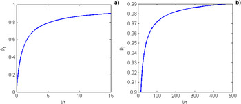
From this solution one can see that βf(t/τ) → 1 for t/τ → ∞, namely the relativistic velocities are obtained if t/τ ≫ 1, which implies a laser pulse duration much larger than τ = ρ0c 2l/(2I) or equivalently It ≫ ρ0c 2l. For an initial density ρ0 = 1 g/cm3, l = 0.1 µm one gets the dimensionless time τ ~ 50 fs and 0.5 fs for I = 1022 W/cm2 and I = 1024 W/cm2 accordingly.
Figure 6 describes the micro-foil velocity βf as a function of the laser pulse duration t in units of τ = ρ0c 2l/(2I), where ρ0 is the initial density, l is the foil thickness and I is the laser intensity [W/cm2].
Micro-foil velocity βf as a function of the laser pulse duration t in units of τ = ρ0c 2l/(2I), where ρ0 is the initial density, l is the foil thickness and I is the laser intensity [W/cm2].

The kinetic energy of the foil W Kf and the ratio between W Kf and the laser energy W L = ItS are given by
 $$\eqalign{{w_{Kf} \over S} &= {\rm \rho}_0 lc^2 \left({1 \over \sqrt{1 - {\rm \beta}_f^2}} - 1 \right) \cr {W_{Kf} \over W_L} &= {\left({1 \over \sqrt{1 - {\rm \beta}_f^2}} - 1 \right)\over \left[\displaystyle{\lpar 2 - {\rm \beta}_f\rpar \sqrt{1 - {\rm \beta}_f^2} \over 6 \left(1 - {\rm \beta}_f \right)^2} - {1 \over 3} \right]}}$$
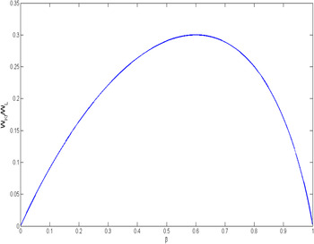
The solution of Eq. (27) imply the asymptotic relativistic behavior W Kf/S ~ t 1/3 for t → ∞ or equivalently for β → 1. On the other domain the non-relativistic limit W Kf/S ~ t 2 is obtained for t → 0. According to the ratio W Kf/W L one can see that the maximum efficiency to accelerate a foil is 30% for a flyer velocity of about 0.6c.
5. DISCUSSION
Due to the recent developments in high power lasers (Tajima & Mourou, Reference Tajima and Mourou2002) in the multi-petawatt domain it is suggested in this paper to accelerate micro-foils to relativistic velocities. From Figure 6 we learn that one can get a micro-foil with half the speed of light for a laser pulse duration τ if Iτ = 4.5 × 10⁸ J/cm2 (e.g., 0.5 fs laser with I = 1024 W/cm2) for a flyer with initial density 1 g/cm3 and a foil thickness of 0.1 micron. A cross-section area of 10 µm2 will require laser energy of 45 J.
In this paper, we calculate the high velocities achieved by the laser acceleration of a micro-foil. This high velocity foil collides with a second foil resulting in the creation of the relativistic shock waves. The Hugoniot of these shock waves are explicitly calculated for extreme relativistic and ideal gas equations of state (Eliezer et al., Reference Eliezer, Ghatak and Hora2002; Eliezer & Ricci, Reference Eliezer and Ricci1991). The density, pressure, temperature, and shock wave velocities are calculated for this impact collision. The analytically derived thermodynamic parameters in these collisions are enormous and they might exist only in astrophysical phenomena or nuclear collisions.
In order to know exactly the shock states achieved in the collision, the initial flyer density and pressure are required. Since the scale of acceleration is on the order of 1 fs one gets a change in density less than 20% (the relative initial volume change is of the order 2v pt/l, where the plasma thermal velocity is less than 109 cm/s). Regarding the initial pressure we can see from Figure 1 that for a shock wave with a pressure increase larger than 1000 the influence of the initial pressure (although high in absolute values) is negligible. Furthermore we suggest measuring experimentally the flyer velocity using the relativistic Doppler effect, while the initial density could be estimated experimentally using an X-ray pulse created by a secondary laser beam.
Regarding the equation of state, it is important to emphasis that we chose the above EOS because they are frequently used in the literature. Only the experiments will tell what the appropriate EOS for different materials is. Furthermore, the ideal gas relation between the pressure P and the temperature T, P = nk BT is a good relativistic equation for particles with a zero chemical potential (Eliezer et al., Reference Eliezer, Ghatak and Hora2002), however the equation relating the internal energy e with the pressure e = ρc 2 + P/(Γ − 1) is not a proper relativistic EOS. Therefore our analysis with this equation has to be considered only on a phenomenological basis.
Another important issue is the question if the hydrodynamic instabilities will break the foil before impact. First, because the relativistic effects the instability grows in the exponent in the laboratory frame is γ times slower than in the plasma reference frame (Esirkepov et al., Reference Esirkepov, Borghesi, Bulanov, Mourou and Tajima2004). Second, the radiation pressure causes a stretching of the plasma surface so that the instability is significantly reduced. A comprehensive discussion of this instability is given by Weinberg (Reference Weinberg1972) in analyzing the formation of galaxies and their expansion stability to radiation. The conclusion is that the instability increase is proportional to time but not an exponential growth. Furthermore, in the model that laser ponderomotive potential creates a charge separation between the electrons and the ions (a double layer) where the ions are accelerated forward, surface tension stabilization may occur (Eliezer & Hora, Reference Eliezer and Hora1989). In this case, our flyer is accelerated forward with a double layer on its solid-vacuum surface (Naumova et al., Reference Naumova, Schlegel, Tikhonchuk, Labaune, Sokolov and Mourou2009; Hora et al., Reference Hora, Lalousis and Eliezer1984). Taking all this into account for a femtosecond acceleration time it seems conceivable that during this short time before it collides with a second foil the flyer will not break.
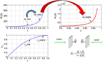
The laser energy can be reduced significantly if we use two lasers in order to accelerate two micro-foils in opposite directions, thus causing them to collide. According to the law of the addition of relativistic velocities, the relative impact velocity between the foils is given by (β1 + β2)/(1 + β1β2). For example if β1 = β2 = 0.8 then the impact relative velocity is 0.9756c; implying a very large reduction of energy according to Figures 7 and 8. This phenomenon can be easily understood when looking at the asymptotic relativistic behavior of the foil kinetic energy per unit area W Kf/S. This specific energy varies as t 1/3 for t → ∞ and as t 2 for t → 0, so that the power law changes from 2 to 1/3 asymptotically. Therefore it is important to emphasize that the requirement for the laser energy W L > >ItS is changed to W L ~ ItS for the impact collision of two accelerated micro-foils.
The ratio of the flyer kinetic energy to the laser energy as a function of the flyer velocity.

The advantage of two micro-foil collisions.

Today particles must be accelerated along many kilometers in order to achieve high energies. In our scheme the foils are accelerated to relativistic velocities through a distance of the order of one millimeter or less. We propose that these relativistic collisions of two micro-foils accelerated by future lasers may offer a new way of accelerating particles or nuclei in the laboratory as suggested in Figure 8. The advantage of accelerating two flyers to lower relativistic velocities on the order of 0.8c would lead to significantly higher relativistic velocities and accordingly more relativistic shock waves.