



1. Introduction
The modeling of portfolio losses has become a critical aspect of risk management and solvency assessment in the insurance industry. The study of multidimensional risk models has garnered significant scholarly attention in recent years, as one-dimensional risk models often fail to capture the whole picture of effects on an insurer’s solvency, especially for insurers managing multiple business lines with dependent claims. In practical financial markets and the insurance industry, major events such as pandemics, earthquakes, and storms significantly affect multiple business lines. These events lead not only to direct property losses and medical compensations but also to secondary consequences over time. Substantial research has been conducted on risk models with delayed claims, providing insights into how primary and subsequent impacts affect insurance companies.
The exploration of risk models incorporating delayed claims began with the seminal work of Waters and Papatriandafylou [Reference Waters and Papatriandafylou35], which introduced a discrete-time risk model with delays in claim settlements. This foundational work spurred extensive studies in the field of insurance, leading to the development of both discrete-time and continuous-time models; see [Reference Xiao and Guo36, Reference Yuen and Guo42], and [Reference Li and Wu20] for discrete-time risk models, and [Reference Meng and Wang25, Reference Xie and Zou37, Reference Zou38, Reference Yuen, Guo and Ng41], and [Reference Zou and Xie45] for continuous-time risk models, among many others. These studies adopted the light-tailed claim assumption, which is appropriate for modeling small claims. However, empirical evidence from [Reference Embrechts, Klüppelberg and Mikosch9] and [Reference McNeil, Frey and Embrechts24] demonstrates that most insurance claims, particularly large ones, exhibit heavy-tailed characteristics. We refer the reader to [Reference Fu and Li11, Reference Gao, Zhuang and Huang12, Reference Yang and Li39, Reference Zhang, Liu and Yang44], and [Reference Liu, Chen and Fu23] for recent literature on the ruin estimation of risk models with delayed claims following heavy-tailed distributions.
Most existing delayed claim models assume that each main claim is accompanied by only one delayed claim, which contradicts real-world scenarios where extreme events typically trigger multiple claims of both types. Recent studies have developed more realistic risk models incorporating random numbers of delayed claims. Li [Reference Li18] proposed a one-dimensional renewal risk model allowing for random delayed claims, and derived asymptotic estimates of ruin probabilities for subexponential and extended regular varying claim sizes. Liu et al. [Reference Liu, Gao and Dong22] further developed a risk model with dependent main and delayed claims, deriving asymptotic estimates of ruin probabilities for heavy-tailed cases.
When an insurer manages multiple business lines, catastrophic events may trigger multiple main claims requiring immediate settlement (e.g. property damage and death compensation), followed by a random number of delayed claims (e.g. medical reimbursements and subsequent treatments) arising after stochastic delays. To capture these characteristics, we introduce a multidimensional risk model with heavy-tailed claims to characterize the surplus of the insurer operating multiple lines:
 \begin{equation} \left(\begin{array}{c} U_1(t) \\ \vdots \\ U_d(t) \end{array}\right)=\left(\begin{array}{c} \rho_1 x \mathrm{e}^{R_{t}} \\ \vdots \\ \rho_d x \mathrm{e}^{R_{t}} \end{array}\right)+\left(\begin{array}{c} \int_0^t \mathrm{e}^{R_{t-s}}C_{1}(\mathrm{d} s) \\ \vdots \\ \int_0^t \mathrm{e}^{R_{t-s}} C_{d}(\mathrm{d} s) \end{array}\right)-\left(\begin{array}{c} S_{1}(t) \\ \vdots \\ S_{d}(t) \end{array}\right),\end{equation}
where
 \begin{align*}S_{k}(t)=\sum_{i=1}^{N_{k}(t)}\left( X_{k i} \mathrm{e}^{R_{t-\tau_{ki}}}+ \sum_{j=1}^{M_{ki}}Y_{kij} \mathrm{e}^{R_{t-\tau_{ki}-D_{kij}}}\mathbb{I}_{\{\tau_{ki}+D_{kij}\leq t\}}\right)\end{align*}
denotes the discounted aggregate claim of the kth business line by time t for
 $k=1,\ldots,d$
,
 $\left\{\left(U_1(t), \ldots, U_d(t)\right) ,\, t \geq 0\right\}$
the multidimensional surplus process,
 $\left(\rho_1 x, \ldots, \rho_d x\right)$
the vector of initial surpluses assigned to different business lines with
 $x>0$
and
 $\rho_1, \ldots, \rho_d>0$
such that
 $\sum_{k=1}^d \rho_k=1$
,
 $\left\{\boldsymbol{C}(t)=\left(C_1(t), \ldots, C_d(t)\right),\, t \geq 0\right\}$
the vector of the premium accumulation processes,
 $\left\{\boldsymbol{X}_{i}=\left(X_{1 i}, \ldots, X_{d i}\right) ,\, i\in \mathbb{N}_{+}\right\}$
the sequence of main claim size vectors,
 $\left\{\boldsymbol{Y}_{ij}=(Y_{1 ij}, \ldots, Y_{d ij}) ,\: i,j\in \mathbb{N}_{+}\right\}$
the sequence of delayed claim size vectors,
 $\{M_{ki},\: k=1,\ldots,d, \, i\in \mathbb{N}_{+}\}$
the sequence of random numbers for delayed claims, and
 $\mathbb{I}_{A}$
the indicator function for an event A. For each
 $ i\in \mathbb{N}_{+}$
,
 $X_{k i}$
describes the ith main claim of the kth business line arriving at time
 $\tau_{k i}$
. Assume that the main claim
 $X_{k i}$
is accompanied by delayed claims
 $Y_{ki1},\ldots,Y_{kiM_{ki}}$
, where
 $Y_{kij}$
describes the corresponding delayed claim arriving at time
 $\tau_{k i}+D_{k ij}$
for
 $j= 1,\ldots,M_{ki}$
, with
 $D_{k ij}$
denoting a random delay time. The arrival time vectors
 $\left\{\left(\tau_{1 i}, \ldots, \tau_{d i}\right),\, i \in \mathbb{N}\right\}$
constitute a claim-number vector process
 $\{\boldsymbol{N}(t)=(N_1(t), \ldots, N_d(t)),\, t \geq 0\}$
. The price process of the investment portfolio is described as a geometric Lévy process
 $\left\{\mathrm{e}^{R_t},\, t \geq 0\right\}$
, with
 $\left\{R_t,\, t \geq 0\right\}$
being a Lévy process which starts from 0.
Compared with the one-dimensional case, multidimensional risk models offer various ways of defining the ruin time; see [Reference Cai and Li3, Reference Chen, Yuen and Ng6, Reference Hu and Jiang14, Reference Li, Liu and Tang19], among many others, for the study of some commonly used definitions. In this paper, we use two types of ruin times under the multidimensional risk models shown in (1), and the corresponding ruin probabilities with a finite horizon
 $T>0$
can be formulated as
 \begin{align*}\psi_\textrm{max}(x;\,T)=\textrm{P}\bigl(T_\textrm{max} \leq T \mid(U_1(0), \ldots, U_d(0))=(\rho_1 x, \ldots, \rho_d x)\bigr)\end{align*}
and
 \begin{align*}\psi_\textrm{min}(x;\,T)=\textrm{P}\bigl(T_\textrm{min} \leq T \mid(U_1(0), \ldots, U_d(0))=(\rho_1 x, \ldots, \rho_d x)\bigr),\end{align*}
where
 \begin{align*}T_\textrm{max}=\inf \left\{t>0\,:\, \max _{1 \leq k \leq d}\{U_k(t)\}<0\right\},\quad T_\textrm{min}=\inf \left\{t>0\,:\, \min _{1 \leq k \leq d}\{U_k(t)\}<0\right\}.\end{align*}
Accordingly, the infinite-time ruin probability is defined as
 \begin{align*}\psi_{*}(x)=\textrm{P}\bigl(T_{*}<\infty \mid(U_1(0), \ldots, U_d(0))=(\rho_1 x, \ldots, \rho_d x)\bigr),\end{align*}
where
 $*$
may be one of ‘
 $\max$
’ and ‘
 $\min$
’.
Using a multivariate regular variation (MRV) framework for dependent claim sizes, we extend ruin estimation to a multidimensional risk model with a geometric Lévy price process, arbitrarily dependent claim-number processes, and random numbers of delayed claims. Practically, claim sizes may be dependent on macroeconomic conditions and seasonal effects. The MRV structure can help model these dependency characteristics in claims. For example, main claims such as property damage may correlate by region or disaster type, while delayed claims such as medical compensations may depend on age or medical resource availability. Allowing for a random number of delayed claims also enhances realism for extreme events, as predicting the exact number of delayed claims over an uncertain future period is difficult.
The rest of this paper is organized as follows. Section 2 introduces the necessary preliminaries and presents the main results. Section 3 presents numerical studies to evaluate the accuracy of the obtained asymptotic results. Section 4 makes some concluding remarks. The proofs of the lemmas and main results are detailed in Section 5.
2. Preliminaries and main results
For convenience, we introduce the following notation that is used throughout this paper. For two positive functions
 $f({\cdot})$
and
 $g({\cdot})$
, we write
 $f(x) \lesssim g(x)$
or
 $g(x) \gtrsim f(x)$
if
 $\lim \sup _{x \rightarrow \infty} f(x) / g(x) \leq 1$
, write
 $f(x) \sim g(x)$
if both
 $f(x) \lesssim g(x)$
and
 $f(x) \gtrsim g(x)$
, write
 $f(x) = o(g(x))$
if
 $\lim_{x \rightarrow \infty} f(x)/ g(x) = 0$
, and write
 $f(x) \asymp g(x)$
if
 $0<\liminf_{x \rightarrow \infty}f(x)/g(x)<\limsup_{x \rightarrow \infty}f(x)/g(x) <\infty$
. Hereafter, unless otherwise stated, all limit relationships hold as
 $x\rightarrow\infty$
. For any
 $x, y \in \mathbb{R}$
, write
 $x\vee y=\max\{x, y\}$
and
 $x\wedge y = \min\{x, y\}$
.
We now give a brief review of regularly varying distributions. Let
 $\overline{F} = 1-F$
be a distribution on
 $[ 0,\infty )$
with an infinite upper endpoint, i.e.
 $\overline{F}(x) > 0$
for all
 $x \geq 0$
. The distribution F is said to have a regularly varying tail with index
 $\alpha > 0$
, written as
 $F \in \mathcal{R}_{-\alpha}$
, if
 \begin{align*}\lim _{x \rightarrow \infty} \frac{\overline{F}(xy)}{\overline{F}(x)}=y^{-\alpha}\end{align*}
holds for every
 $y>0$
. If
 $F \in \mathcal{R}_{-\alpha}$
, then
 $\overline{F}(x)=x^{-\alpha}l(x)$
where l(x) is a slowly varying function. By Theorem 1.5.6 of [Reference Bingham, Goldie and Teugels2], for any
 $\epsilon>0$
there exists some sufficiently large
 $x_0$
such that
 \begin{align*}(1-\epsilon)\left(\frac{y}{x}\right)^{-\alpha-\epsilon} \leq \frac{\overline{F}(y)}{\overline{F}(x)} \leq(1+\epsilon)\left(\frac{y}{x}\right)^{-\alpha+\epsilon}\end{align*}
holds for all
 $y \geq x \geq x_0$
, and further
 \begin{equation} x^{-(\alpha+\epsilon)}=o\bigl(\overline{F}(x)\bigr).\end{equation}
A natural extension of univariate regular variation is MRV, which has been extensively studied. The MRV framework is valuable for quantitative risk management, providing a useful approach to modeling both the heavy tails of marginal distributions and dependence among loss variables. A detailed discussion can be found in [Reference Resnick28, Reference Resnick29]. See [Reference Konstantinides and Li16, Reference Li17, Reference Tang and Yuan33], and [Reference Cheng, Konstantinides and Wang7] for recent applications of the MRV framework.
By definition, a random vector
 $(X_1, \ldots, X_d)$
is said to follow the structure of MRV, written as
 $(X_1, \ldots, X_d) \in \operatorname{MRV}(\alpha, F, v)$
, if there exist some
 $\alpha>0$
, some distribution
 $F\in \mathcal{R}_{-\alpha}$
, and some Radon measure v on
 $[0, \infty]^d \backslash\{\mathbf{0}\}$
satisfying
 $v([0, \infty]^d \backslash\{\mathbf{0}\})>0$
such that as
 $x \rightarrow \infty$
,
 \begin{align*}\frac{1}{\overline{F}(x)}\, \textrm{P}\left(\frac{(X_1, \ldots, X_d)}{x} \in \cdot\right) \stackrel{\rm v}{\rightarrow} v({\cdot}),\end{align*}
where
 $\stackrel{\rm v}{\rightarrow}$
denotes vague convergence and
 $\textbf{0}=(0,\ldots,0)$
. By Theorem 1.14 of [Reference Lindskog21], the homogeneity
 $v(y K)=y^{-\alpha} v(K)$
holds for any
 $y>0$
and any v-continuous Borel set
 $K \subseteq[0, \infty]^d \backslash\{\mathbf{0}\}$
. Let
 $\textbf{1}=(1,\ldots,1)$
, and let
 $\mathbf{1}_k$
denote the vector with 1 in the kth position and 0 elsewhere. If
 \begin{align*}\lim _{x \rightarrow \infty} \frac{1}{\overline{F}(x)} \,\textrm{P}\left(\bigcap_{k=1}^d\{X_k>x\}\right)=v\bigl((\mathbf{1}, \infty]\bigr)>0,\end{align*}
which implies that the
 $X_1, \ldots, X_d$
are pairwise asymptotically dependent, then the marginal distributions
 $F_{1}, \ldots, F_{d}$
of
 $(X_1, \ldots, X_d)$
satisfy
 \begin{equation} \lim_{x \rightarrow \infty} \frac{\overline{F}_{k}(x)}{\overline{F}(x)}=v\bigl((\mathbf{1}_k, \infty]\bigr)\,=\!:\, c_k>0\quad\mbox{for } k=1, \ldots, d,\end{equation}
which implies that the tails of
 $X_1, \ldots, X_d$
are regularly varying and mutually comparable. For convenience, we write
 \begin{align*}\lim _{x \rightarrow \infty} \frac{1}{\overline{F}(x)} \,\textrm{P}\left(\bigcap_{k=1}^d\{X_k>b_k x\}\right)=v\bigl((b_1, \infty] \times \cdots \times(b_d, \infty]\bigr)\,=\!:\,V(b_1, \ldots,b_d)>0.\end{align*}
The assumption in the previous section that the price process is a geometric Lévy process has been widely applied. See [Reference Wang and Wu34, Reference Yuen, Wang and Wu43], and [Reference Heyde and Wang13] for examples of this assumption on price processes used in mathematical finance and insurance. As for the Lévy process
 $\{R_t,\, t \geq 0\}$
, its Laplace exponent is defined as
 \begin{align*}\phi(z)=\log \textrm{E}\bigl[\mathrm{e}^{-z R_1}\bigr], \quad z \in \mathbb{R}.\end{align*}
If
 $\phi(z)$
is finite, then
 \begin{align*}\textrm{E}\bigl[\mathrm{e}^{-z R_t}\bigr]=\mathrm{e}^{t \phi(z)}<\infty, \quad t \geq 0,\end{align*}
and
 $\phi(z)$
is convex in z. If
 $\phi\left(z_0\right)<0$
for some
 $z_0>0$
, then upon noting that
 $\phi(0)=0$
, it follows that
 $\phi(z)<0$
for any
 $z \in(0, z_0]$
.
2.1. Main results
Recalling the multidimensional model constructed in (1), we provide some basic assumptions regarding the distributions and dependence structures of variables. Throughout, we assume that
 $\{\boldsymbol{N}(t),\, t \geq 0\}$
,
 $\{\boldsymbol{C}(t),\, t \geq 0\}$
,
 $\left\{\boldsymbol{M}_i=\left(M_{1 i}, \ldots, M_{d i}\right),\, i \in \mathbb{N}_{+}\right\}$
,
 $\{D_{kij},\: i,j \in \mathbb{N}_{+}, \,k=1,\ldots,d\}$
,
 $\left\{\boldsymbol{X}_i,\, i \in \mathbb{N}_{+}\right\}$
,
 $\{\boldsymbol{Y}_{ij},\; i,j \in \mathbb{N}_{+}\}$
, and
 $\left\{R_t,\, t \geq 0\right\}$
are mutually independent.
Assumption 1. Let
 $\{\boldsymbol{X}_{i},\, i \in \mathbb{N}_{+}\}$
be a sequence of independent and identically distributed (i.i.d.) copies of a generic nonnegative random vector
 $\boldsymbol{X}=(X_1, \ldots, X_d)$
with generic marginal distribution functions
 $F_{1},\ldots, F_{d}$
, and let
 $\{\boldsymbol{Y}_{ij},\; i,j \in \mathbb{N}_{+}\}$
be a sequence of i.i.d. copies of a generic nonnegative random vector
 $\boldsymbol{Y}=(Y_1, \ldots, Y_d)$
with generic marginal distribution functions
 $G_{1},\ldots, G_{d}$
.
Assumption 2. Let
 $\{\boldsymbol{M}_{i},\, i \in \mathbb{N}_{+}\}$
be a sequence of nonnegative, integer-valued, and i.i.d. copies of a generic random vector
 $\boldsymbol{M}=(M_1, \ldots, M_d)$
with arbitrarily dependent components satisfying
 $\textrm{E}[\mathrm{e}^{\delta M_k}]<\infty$
for some
 $\delta>0$
and all
 $k=1, \ldots, d$
. Let
 $\{D_{kij},\; i,j \in \mathbb{N}_{+}, \, k=1,\ldots,d \}$
be a sequence of i.i.d. copies of a generic nonnegative random variable D with a generic distribution H.
Assumption 3. The premium accumulation vector process
 $\{\boldsymbol{C}(t),\, t \geq 0\}$
has arbitrarily dependent components with
 $\boldsymbol{C}(0)=\mathbf{0}$
and each component having a nondecreasing cadlag path.
Assumption 4. Let
 $\{(\theta_{1 i}, \ldots, \theta_{d i}) ,\, i\in\mathbb{N}_{+}\}$
be a sequence of i.i.d. positive random vectors with arbitrarily dependent components, where for each
 $k=1,\ldots,d$
, the claim interarrival times are such that
 $\theta_{k1} = \tau_{k1}$
and
 $\theta_{ki} = \tau_{ki} - \tau_{k(i-1)}$
for
 $i\geq2$
.
Assumption 4 introduces a general dependence structure among the claim-number processes through inheriting the dependence among the interarrival times
 $\{(\theta_{1 i}, \ldots, \theta_{d i}) ,\, i\in\mathbb{N}_{+}\}$
. Clearly, Assumption 4 implies that each
 $\lbrace N_k(t_k),\, t_k \geq 0\rbrace $
is a renewal process. For
 $(t_1, \ldots, t_d) \in$
 $[0, \infty)^d$
, we write
 \begin{align*}N(t_1, \ldots, t_d) &=\max \{i \in\mathbb{N}\,:\, \tau_{1 i} \leq t_1, \ldots, \tau_{d i} \leq t_d\} =\min _{1 \leq k \leq d}\left\{N_k(t_k)\right\},\\\lambda(t_1, \ldots, t_d) & =\textrm{E}\bigl(N(t_1, \ldots, t_d)\bigr) =\sum_{i=1}^{\infty} \textrm{P}(\tau_{1 i} \leq t_1, \ldots, \tau_{d i} \leq t_d)\end{align*}
and, for any
 $1 \leq k_1\lt \cdots \lt k_l \leq d$
,
 \begin{align*}\lambda_{k_1,\ldots,k_{l}}(t_{1},\ldots,t_{l})=\sum_{i=1}^{\infty} \textrm{P}(\tau_{k_1 i} \leq t_1, \ldots, \tau_{k_l i} \leq t_l).\end{align*}
Now we are ready to present our main results. For the multidimensional risk model with delayed claims given by (1), the following theorem establishes the asymptotic behavior of both the finite-time ruin probabilities
 $\psi_\textrm{max}(x;\,T)$
and
 $\psi_\textrm{min}(x;\,T)$
and their infinite-time counterparts
 $\psi_\textrm{max}(x)$
and
 $\psi_\textrm{min}(x)$
.
Theorem 1. Consider the multidimensional risk model given by (1). Suppose that Assumptions 1–4 hold with
 $\boldsymbol{X}\in\operatorname{MRV}(\alpha, F, \nu)$
and
 $\boldsymbol{Y}\in\operatorname{MRV}(\alpha, G, \mu)$
such that
 $\nu((\mathbf{1}, \infty])>0$
,
 $\mu((\mathbf{1}, \infty])>0$
for some
 $\alpha>1$
and
 $\overline{G}(x)\sim c\overline{F}(x)$
for some constant
 $c>0$
. For any fixed
 $T>0$
,
 $\textrm{P}\bigl(\int_{0}^{t}\mathrm{e}^{-R_{s}}C_{k}(\mathrm{d}s)>x\bigr)=o\bigl(\overline{F}(x)\bigr)$
for any fixed
 $t\in[0,T]$
and
 $k=1, \ldots, d$
. If there exists some
 $\delta>0$
such that
 $\phi(\alpha+\delta)<0$
, then for any fixed
 $T>0$
with
 $\lambda(T, \ldots, T)>0$
,
 \begin{align} \psi_\textrm{max}(x;\, T)&\sim\overline{F}(x)\int_{[0,T]^{d}}\textrm{E}\left[ V_{1}\big(\rho_{1}\mathrm{e}^{R_{t_{1}}},\ldots,\rho_{d}\mathrm{e}^{R_{t_{d}}}\bigr) \right]\lambda(\mathrm{d}t_{1},\ldots,\mathrm{d}t_{d})\nonumber\\[4pt] &\quad +\overline{G}(x)\,\textrm{E}\!\left[ \bigwedge_{k=1}^{d} M_{k}\right]\!\int_{\Omega_{*}}\!\!\textrm{E}\left[ V_{2}\big(\rho_{1}\mathrm{e}^{R_{t_{1}+u_{1}}},\ldots,\rho_{d}\mathrm{e}^{R_{t_{d}+u_{d}}}\big) \right]\lambda(\mathrm{d}t_{1},\ldots,\mathrm{d}t_{d})\!\prod_{i=1}^{d}\!H(\mathrm{d}u_{i}) \end{align}
and
 \begin{align} \psi_\textrm{min}(x;\,T)& \sim \overline{F}(x)\sum_{l=1}^d \sum_{1 \leq k_1 \lt \cdots \lt k_l \leq d}\!({-}1)^{l+1}\!\int_{[0,T]^{l}}\textrm{E}\!\left[\!V_{1}\left(\sum_{m=1}^l \rho_{k_m}\mathrm{e}^{R_{t_{m}}} \mathbf{1}_{k_m}\right)\right] \lambda_{k_1,\ldots,k_{l}}(t_{1},\ldots,t_{l})\nonumber \\ &\quad + \overline{G}(x)\,\textrm{E}\left[\bigwedge_{k=1}^{d} M_{k}\right]\sum_{l=1}^d \sum_{1 \leq k_1 \lt \cdots \lt k_l \leq d} ({-}1)^{l+1} \nonumber \\ & \qquad\qquad\qquad\quad\times \int_{\Omega_{*}^{l}}\!\textrm{E}\!\left[ V_{2}\!\left(\sum_{m=1}^l \rho_{k_m}\mathrm{e}^{R_{t_{m}+u_{m}}} \mathbf{1}_{k_m}\right) \right] \lambda_{k_1,\ldots,k_{l}}(t_{1},\ldots,t_{l})\prod_{i=1}^{l}H(\mathrm{d}u_{i}), \end{align}
where we write
 $\Omega_{*}^{l}=\lbrace (t_{1},\ldots,t_{l},u_{1},\ldots,u_{l})\in[0,T]^{2l}\,:\,0 \lt t_{k}+u_{k}\leq T \ \text{for}\ k=1,\ldots, l\rbrace$
, with
 $\Omega_{*}^{d}=\Omega_{*}$
in particular,
 $V_{1} (\boldsymbol{x})=V_{1} (x_{1},\ldots,x_{d}) =\nu((\boldsymbol{x},\boldsymbol{\infty}] )$
and
 $V_{2} (\boldsymbol{x}) = V_{2} (x_{1},\ldots,x_{d}) = \mu((\boldsymbol{x},\boldsymbol{\infty}])$
. Specifically, if
 $\textrm{P}\bigl(\int_{0}^{\infty}\mathrm{e}^{-R_{s}}C_{k}(\mathrm{d}s)>x\bigr)=o\bigl(\overline{F}(x)\bigr)$
, then relations (4) and (5) hold for
 $T=\infty$
.
Remark 1. Recall that for the Lévy process
 $\{R_t,\, t \geq 0\}$
, the condition
 $\phi(\alpha + \delta) < 0$
for some
 $\delta > 0$
implies
 $\phi(z) < 0$
for all
 $z \in (0, \alpha + \delta]$
. By Jensen’s inequality, this further yields
 $\textrm{E}[R_1] > 0$
. As shown in [Reference Tang, Wang and Yuen32], the condition
 $\phi(\alpha + \delta) < 0$
means that the impact of insurance claims dominates that of financial uncertainty. This interpretation is further supported by the relations (4) and (5), which indicate that the tail behavior of the claim-size distributions
 $F$
and
 $G$
determines the exact decay rate of the ruin probabilities, whereas financial uncertainty and claim frequency contribute only to the coefficient in the asymptotic formulas.
Following the proof of Theorem 1, the finite-time ruin probability results can be extended to the case where arbitrarily dependent nonrenewal counting processes satisfy certain moment conditions and the Laplace exponent satisfies
 $\phi(\alpha+\delta)<\infty$
for some
 $\delta>0$
.
Corollary 1. In addition to the other conditions of Theorem 1, except for Assumption 4 and
 $\phi(\alpha+\delta)<0$
for some
 $\delta>0$
, assume that the counting processes
 $N_1(t), \ldots, N_d(t)$
are arbitrarily dependent and not necessarily renewal processes satisfying
 $\textrm{E}[\mathrm{e}^{\kappa N_k(T)}]<\infty$
for all
 $k=1, \ldots, d$
, any fixed
 $T>0$
and some
 $\kappa>0$
. If there exists some
 $\delta>0$
such that
 $\phi(\alpha+\delta)<\infty$
, then the estimates of finite-time ruin probabilities
 $\psi_\textrm{max}(x;\,T)$
and
 $\psi_\textrm{min}(x;\,T)$
shown in (4) and (5) hold.
In particular, if the businesses share a common claim-number process and the insurer makes risk-free investments, i.e.
 $N_1(t) \equiv \cdots \equiv N_d(t) \equiv N(t)$
and
 $R_{t}\equiv rt$
, the estimations can be rewritten in a more elegant and transparent form. Here,
 $r\geq0$
suffices for the finite-time ruin probability, and
 $r>0$
is required for the convergence of the relevant quantities in the infinite-time case.
Corollary 2. In addition to the other conditions of Theorem 1, if
 $N_1(t) \equiv \cdots \equiv N_d(t) \equiv N(t)$
with
 $\lambda(t)=\textrm{E}(N(t)) $
and
 $R_{t}\equiv rt$
where
 $r\geq0$
, then
 \begin{align*} \psi_\textrm{max}(x;\,T)& \sim\overline{F}(x)\left(\int_{0-}^T \mathrm{e}^{-\alpha r t} \lambda(\mathrm{d} t)\right) V_{1}(\rho_{1},\ldots,\rho_{d})\\ &\quad +\overline{G}(x)\,\textrm{E}\left[ \bigwedge_{k=1}^{d} M_{k}\right]\int_{\bar{\Omega}_{*}^{d}}\mathrm{e}^{-\alpha r t} V_{2}(\rho_{1}\mathrm{e}^{ru_{1}},\ldots,\rho_{d}\mathrm{e}^{ru_{d}})\lambda(\mathrm{d} t)\prod_{i=1}^{d}H(\mathrm{d}u_{i}) \end{align*}
and
 \begin{align*} \psi_\textrm{min}(x;\,T)& \sim\overline{F}(x)\sum_{l=1}^d \sum_{1 \leq k_1\lt \cdots\lt k_l \leq d}({-}1)^{l+1}\left(\int_{0-}^T \mathrm{e}^{-\alpha r t} \lambda(\mathrm{d} t)\right) V_{1}\left(\sum_{m=1}^l \rho_{k_m}\mathbf{1}_{k_m}\right)\\ &\quad+ \overline{G}(x)\,\textrm{E}\left[ \bigwedge_{k=1}^{d} M_{k}\right]\sum_{l=1}^d \sum_{1 \leq k_1\lt \cdots\lt k_l \leq d}({-}1)^{l+1} \\ & \qquad\qquad\qquad\qquad\qquad\quad\times \int_{\bar{\Omega}_{*}^{l}}\mathrm{e}^{-\alpha r t} V_{2}\left(\sum_{m=1}^l \rho_{k_m}\mathrm{e}^{ru_{m}} \mathbf{1}_{k_m}\right)\lambda(\mathrm{d} t)\prod_{i=1}^{l}H(\mathrm{d}u_{i}), \end{align*}
where
 $\bar{\Omega}_{*}^{l}=\lbrace (t,u_{1},\ldots,u_{l})\in[0,T]^{l+1}\,:\, 0< t+u_{k}\leq T,\, k=1,\ldots, l\rbrace$
. Further, if
 $r>0$
, then for
 $T=\infty$
we have
 \begin{align*} \psi_\textrm{max}(x) &\sim \overline{F}(x)\frac{\textrm{E}(\mathrm{e}^{-\alpha r \theta})}{1-\textrm{E}(\mathrm{e}^{-\alpha r \theta})} V_{1}(\rho_1, \ldots, \rho_d)\\ &\quad+\overline{G}(x)\,\textrm{E}\left[ \bigwedge_{k=1}^{d} M_{k}\right]\frac{\textrm{E}(\mathrm{e}^{-\alpha r \theta})}{1-\textrm{E}(\mathrm{e}^{-\alpha r \theta})}\int_{[0,\infty)^{d}} V_{2}(\rho_{1}\mathrm{e}^{ru_{1}},\ldots,\rho_{d}\mathrm{e}^{ru_{d}})\prod_{i=1}^{d}H(\mathrm{d}u_{i}) \end{align*}
and
 \begin{align*} \psi_\textrm{min}(x)&\sim\overline{F}(x)\frac{\textrm{E}(\mathrm{e}^{-\alpha r \theta})}{1-\textrm{E}(\mathrm{e}^{-\alpha r \theta})} \sum_{l=1}^d \sum_{1 \leq k_1\lt \cdots\lt k_l \leq d}({-}1)^{l+1}V_{1}\left(\sum_{m=1}^l \rho_{k_m}\mathbf{1}_{k_m}\right)\\ &\quad + \overline{G}(x)\,\textrm{E}\left[ \bigwedge_{k=1}^{d} M_{k} \right]\frac{\textrm{E}(\mathrm{e}^{-\alpha r \theta})}{1-\textrm{E}(\mathrm{e}^{-\alpha r \theta})}\sum_{l=1}^d\sum_{1 \leq k_1\lt \cdots \lt k_l \leq d} ({-}1)^{l+1} \\ &\qquad\qquad\qquad\qquad\qquad\qquad\qquad\times \int_{[0,\infty)^{l}}V_{2}\left(\sum_{m=1}^l \rho_{k_m}\mathrm{e}^{ru_{m}} \mathbf{1}_{k_m}\right)\prod_{i=1}^{l}H(\mathrm{d}u_{i}), \end{align*}
where
 $\theta$
is the generic random variable for the interarrival times of the renewal process N(t).
3. Numerical studies
In this section, we examine the accuracy of the asymptotic estimates. Recalling the multidimensional risk model given by (1), we compare the values of the ruin probabilities
 $\psi_\textrm{max}(x;\,T)$
and
 $\psi_\textrm{min}(x;\,T)$
obtained by crude Monte Carlo (CMC) simulation with asymptotic estimates from Corollary 2. For
 $T>0$
, the ruin probabilities can be estimated by the simulated estimations
 \begin{align*}\hat{\psi}_\textrm{max}(x;\,T)=\frac{1}{N} \sum_{j=1}^N \mathbb{I}_{\Bigl\lbrace \bigcap_{k=1}^{d}\Bigl(\min\limits_{m=1, \ldots, n} U_{k}^{(j)}(t_m)<0\Bigr)\Bigr\rbrace}\end{align*}
and
 \begin{align*}\hat{\psi}_\textrm{min}(x;\,T)=\frac{1}{N} \sum_{j=1}^N \mathbb{I}_{\Bigl\lbrace \bigcup_{k=1}^{d} \Bigl(\min\limits_{m=1, \ldots, n} U_{k}^{(j)}(t_m)<0\Bigr)\Bigr\rbrace},\end{align*}
where
 $U_{k}^{(j)}(t_m)$
is the surplus of the kth line at time
 $t_m$
for path j and
 $t_m=mT/ n$
for
 $ m=1, \ldots, n$
. Throughout this section, the simulation is conducted with
 $n=10$
.
Assume that the main claim-size vector
 $\boldsymbol{X}\in\operatorname{MRV}(\alpha, F, \nu)$
and the delayed claim-size vector
 $\boldsymbol{Y}\in\operatorname{MRV}(\alpha, G, \mu)$
, where the distributions F and G both follow the same Pareto distribution for shape
 $\alpha=1.5$
and scale
 $\gamma=1$
, that is,
 \begin{align*} F(x)=G(x)=1-\left( \frac{\gamma}{x+\gamma}\right) ^{\alpha},\quad x>0.\end{align*}
We consider the case where an insurance company operates three lines of business. Recalling
 $c_{k}$
defined in (3), we assume that
 $c_{1}=1$
,
 $c_{2}=0.9$
, and
 $ c_{3}=1.3$
for F and that
 $c_{1}=c_{2}=c_{3}=1$
for G.
We propose to use the Gumbel–Hougaard family of Archimedean copulas to model the dependence among the claim sizes. For a detailed discussion on copulas, we refer the reader to [Reference Nelsen26]. A copula C is said to be Archimedean if it has the following form for
 $(u_{1}, \ldots, u_{d})\in[0,1]^{d}$
:
 \begin{equation} C(u_1, \ldots, u_d)=\varphi^{-1}\bigl(\varphi(u_1)+\cdots+\varphi(u_d)\bigr),\end{equation}
where the generator
 $\varphi\,:\,(0,1)\rightarrow(0,\infty)$
is a strictly decreasing and convex function such that
 $\varphi(0{+})=\infty$
and
 $\varphi(1{-})=0$
, and the function
 $\varphi^{\leftarrow}(y)=\inf \{t \in[0,1]\,:\, \varphi(t) \leq y\}$
is the generalized inverse of
 $\varphi$
. A necessary and sufficient condition for (6) to specify a copula is that the function
 $\varphi^{\leftarrow}$
be complete monotone, that is,
 \begin{align*}({-}1)^k \frac{\mathrm{d}^k}{\mathrm{d} t^k} \,\varphi^{\leftarrow}(t) \geq 0,\quad\mbox{for } k=0,1, \ldots.\end{align*}
Assume that the generator
 $\varphi$
satisfies
 \begin{equation} \lim _{u \downarrow 0} \frac{\varphi(1-t u)}{\varphi(1-u)}=t^\beta, \quad t>0,\end{equation}
for some constant
 $\beta$
. If
 $\beta$
exists, it must satisfy
 $1 \leq \beta \leq \infty$
. See [Reference Charpentier and Segers4] for a list of bivariate Archimedean copulas satisfying the relation (7). By Lemma 5.3 of [Reference Tang and Yuan33], we employ an Archimedean copula of form (6) with generator
 $\varphi(t)=({-}\ln t)^{\beta}$
, where
 $\beta=2\in(1,\infty]$
, to characterize the dependence structure within
 $\boldsymbol{X}$
, as well as that within
 $\boldsymbol{Y}$
. For
 $\mathbf{t}>\mathbf{0}$
, we have
 \begin{align*}\nu( [\mathbf{0}, \mathbf{t}]^c) =\left(\sum_{i=1}^d\left(c_i t_i^{-\alpha}\right)^\beta\right)^{1 / \beta}\quad\!\! \text{and} \quad \nu( (\mathbf{t}, \boldsymbol{\infty}]) =\sum_{\varnothing \neq I \subset\{1, \ldots, d\}}({-}1)^{|I|-1}\left(\sum_{i \in I}\left(c_i t_i^{-\alpha}\right)^\beta\right)^{1 / \beta}.\end{align*}
Similarly, we have
 \begin{align*}\mu( [\mathbf{0}, \mathbf{t}]^c) =\left(\sum_{i=1}^d\left(t_i^{-\alpha}\right)^\beta\right)^{1 / \beta}\quad \text{and} \quad \mu( (\mathbf{t}, \boldsymbol{\infty}]) =\sum_{\varnothing \neq I \subset\{1, \ldots, d\}}({-}1)^{|I|-1}\left(\sum_{i \in I}\left(t_i^{-\alpha}\right)^\beta\right)^{1 / \beta},\end{align*}
where
 $ |I|$
is the cardinality of the set I.
In particular, assume that all business lines share the common counting process
 $\{N(t),$
 $t \geq 0\}$
, where both the interarrival time
 $\theta$
and the delay time D follow an exponential distribution with rate 1. Let the random numbers
 $M_{1i}=M_{2i}=M_{3i}=M_{i}$
almost surely, and suppose that
 $\{M_{i},\, i\in \mathbb{N}_{+}\}$
are i.i.d. copies of a random variable M taking values 1 or 2 with equal probability. The premium accumulation process follows
 $C(t)=ct$
with constant rate
 $c=12$
. The remaining parameters are set to
 $T=10$
, the constant force of interest is
 $r=0.05$
, and the allocation is taken to be
 $\rho_{1}=0.3$
,
 $\rho_{2}=0.3$
, and
 $ \rho_{3}=0.4$
. Then we have
 \begin{align*} \psi_\textrm{max}(x;\,T)&\sim\overline{F}(x)\left(\int_{0-}^T \mathrm{e}^{-\alpha r t} \,\mathrm{d} t\right) \sum_{\varnothing \neq I \subset\{1, 2, 3\}}({-}1)^{|I|-1}\left(\sum_{i \in I}\left(c_i \rho_{i}^{-\alpha}\right)^\beta\right)^{1 / \beta}\\ &\quad +\overline{G}(x)\,\textrm{E}\!\left[\bigwedge_{k=1}^{3} M_{k}\right]\!\int_{\bar{\Omega}_{*}}\!\mathrm{e}^{-\alpha r t}\!\sum_{\varnothing \neq I \subset\{1,2, 3\}}\!({-}1)^{|I|-1}\!\left(\!\sum_{i \in I}\rho_{i}\mathrm{e}^{-\alpha\beta ru_{i}}\!\right)^{1/\beta}\!\mathrm{d}t\!\prod_{i=1}^{3}\mathrm{e}^{-u_{i}}\mathrm{d}u_{i}\end{align*}
and
 \begin{align*} \psi_\textrm{min}(x;\,T)& \sim\overline{F}(x)\left(\int_{0-}^T \mathrm{e}^{-\alpha r t} \,\mathrm{d} t\right)\left(\sum_{i=1}^3\left(c_i \rho_{i}^{-\alpha}\right)^\beta\right)^{1 / \beta}\\ &\quad +\overline{G}(x)\,\textrm{E}\left[\bigwedge_{k=1}^{3} M_{k}\right]\int_{\bar{\Omega}_{*}}\mathrm{e}^{-\alpha r t}\left(\sum_{i=1}^3\rho_{i}\mathrm{e}^{-\alpha\beta ru_{i}}\right)^{1 / \beta}\mathrm{d}t\prod_{i=1}^{3}\mathrm{e}^{-u_{i}}\,\mathrm{d}u_{i},\end{align*}
where
 $\bar{\Omega}_{*}=\lbrace (t,u_{1},\ldots,u_{3})\in[0,T]^{4}\,:\,0 \lt t+u_{k}\leq T, \, k=1,2,3\rbrace$
.
In Table 1, we compare the asymptotic estimates for
 $\psi_\textrm{max}(x;\, T)$
and
 $\psi_\textrm{min}(x;\, T)$
with simulations based on
 $N = 10^6$
. The results show that the asymptotic estimates closely match the simulation data, confirming their accuracy. The error is generally less than 5%, with fluctuations attributed to the limitations of the CMC method. A larger sample size may help offset the negative effects of extremely small ruin probabilities, leading to better simulation results.
Comparision of simulation and approximation of ruin probabilities for
 $\psi_\textrm{max}(x;\,T)$
and
 $\psi_\textrm{min}(x;\,T)$

Table 1 Long description
The table presents a comparison of asymptotic estimates for psi max and psi min with simulation data based on a sample size of 10^6. It includes columns for x values ranging from 500 to 4000, estimated psi max and psi min values, their ratios, and simulated psi max and psi min values. The table shows that the asymptotic estimates closely match the simulation data, with errors generally less than 5%. Notable trends include the increasing values of psi max and psi min as x increases, and the ratios remaining relatively stable around 1. The data suggests that the asymptotic estimates are accurate and reliable for predicting ruin probabilities.
4. Concluding remarks
In this paper we have proposed a multidimensional risk model with stochastic returns driven by a geometric Lévy process, in which each main claim may generate a random number of delayed claims. Using MRV for claim sizes and allowing arbitrarily dependent claim-number processes, we have derived asymptotic results for both infinite-time and finite-time ruin probabilities, which provide new insights into how heavy-tailed risks and claim dependencies affect insurers’ solvency across multiple business lines.
Several promising directions are worthy of pursuit in the future. First, under our assumption on claim sizes, the components are asymptotically dependent with comparable tails. Intuitively, if any component of the claim vector is sufficiently smaller than the others, the claim vector’s contribution to the aggregate risk is considered negligible. In realistic cases, however, jointly multivariate regularly varying tails may not share the same index, which motivates the study of asymptotic independence losses and second-order asymptotic analyses. In this regard, the theory of hidden regular variation (see, for example, Section 9.4 of [Reference Resnick29]) offers valuable tools. Second, it would be desirable to extend the model to broader multivariate distribution classes relevant to insurance applications, particularly multivariate subexponential distributions. The works [Reference Cline and Resnick8, Reference Omey27], and [Reference Samorodnitsky and Sun30] shed some light in this direction. Finally, multidimensional models naturally accommodate richer notions of ruin. By considering multiple common definitions of ruin probabilities, as well as various ruin sets that adapt to varying regulatory requirements, one could capture more practical aspects of solvency assessment in insurance applications.
5. Proofs
5.1. Lemmas
Before proving our main results, we present several useful lemmas. Inspired by Lemma 3.2 of [Reference Konstantinides and Li16] and Theorem 1 of [Reference Fougeres and Mercadier10], we establish an asymptotic result for the joint tail probability of the randomly weighted sums under the MRV structure. For simplicity, write
 $V_{1}(u_{1},\ldots,u_{d})=V_{1}(\boldsymbol{u})=\nu((\boldsymbol{u},\boldsymbol{\infty}])$
and
 $V_{2}(u_{1},\ldots,u_{d})=V_{2}(\boldsymbol{u})=\mu((\boldsymbol{u},\boldsymbol{\infty}])$
.
Lemma 1. Let
 $\left\{\boldsymbol{X}_{i},\, i\in\mathbb{N}_{+}\right\}$
and
 $\left\{\boldsymbol{Y}_{ij},\; i,j\in\mathbb{N}_{+}\right\}$
satisfy Assumption 1. Assume that
 $\boldsymbol{X}\in\operatorname{MRV}(\alpha, F, \nu)$
and
 $\boldsymbol{Y}\in\operatorname{MRV}(\alpha, G, \mu)$
such that
 $\nu((\mathbf{1}, \infty])>0$
and
 $\mu((\mathbf{1}, \infty])>0$
for some
 $\alpha>0$
, and suppose that
 $\overline{G}(x)\sim c\overline{F}(x)$
for some constant
 $c>0$
. Let
 $\{\boldsymbol{\xi}_{i}=(\xi_{1 i}, \ldots, \xi_{d i}),\, i \in \mathbb{N}_{+}\}$
and
 $\{\boldsymbol{\eta}_{ij}=(\eta_{1ij}, \ldots, \eta_{dij}),\; i,j \in \mathbb{N}_{+}\}$
be two sequences of nonnegative and arbitrarily dependent random vectors satisfying
 $\textrm{E}[\xi_{ki}^{\alpha+\delta_{1}}]<\infty$
and
 $\textrm{E}[\eta_{kij}^{\alpha+\delta_{2}}]<\infty$
for some
 $\delta_{1}, \delta_{2}> 0$
, all
 $k=1,\ldots,d$
and
 $i,j\in \mathbb{N}_{+}$
. Assume that
 $\lbrace \boldsymbol{\xi}_{i},\boldsymbol{\eta}_{ij},\;i,j\in\mathbb{N}_{+}\rbrace $
,
 $\{\boldsymbol{X}_{i},\,i\in\mathbb{N}_{+}\}$
and
 $\{\boldsymbol{Y}_{ij},\;i,j\in\mathbb{N}_{+}\}$
are mutually independent. Then for any
 $n_{k}\in\mathbb{N}_{+}$
and
 $m_{ki}\in\mathbb{N}_{+}$
,
 \begin{equation} \begin{aligned} &\textrm{P}\left(\bigcap_{k=1}^{d}\left\lbrace \sum_{i=1}^{n_{k}}\left(\xi_{k i}X_{k i}+\sum_{j=1}^{m_{ki}}\eta_{kij}Y_{k ij}\right)>\rho_{k}x \right\rbrace \right)\\ & \quad \sim \overline{F}(x)\sum_{i=1}^{\hat{n}}\textrm{E}\left[V_{1}\left(\dfrac{\rho_{1}}{\xi_{1i}},\ldots,\dfrac{\rho_{d}}{\xi_{di}}\right)\right]+\overline{G}(x)\sum_{i=1}^{\hat{n}}\sum_{j=1}^{\hat{m}_{i}}\textrm{E}\left[V_{2}\left(\dfrac{\rho_{1}}{\eta_{1ij}},\ldots,\dfrac{\rho_{d}}{\eta_{dij}}\right)\right], \end{aligned} \end{equation}
where
 $\hat{n}=\min\limits_{k=1,\ldots,d}\left\lbrace n_{k}\right\rbrace $
and
 $\hat{m}_{i}=\min\limits_{k=1,\ldots,d}\left\lbrace m_{ki}\right\rbrace $
.
Proof. Let
 $\check{n}=\max \limits_{k=1,\ldots,d}\{n_k\}$
and
 $\check{m}_{i}=\max\limits_{k=1,\ldots,d}\{m_{ki}\}$
. Note that
 $\{\boldsymbol{X}_{i},\, i\in\mathbb{N}_{+}\}$
and
 $\{\boldsymbol{Y}_{ij},\;i,j\in\mathbb{N}_{+}\}$
are mutually independent. By Assumption 1, Lemma 7.2 of [Reference Resnick29], and the fact that
 $\overline{G}(x)\sim c\overline{F}(x)$
, we have the
 $\sum_{k=1}^{d}( n_{k}+\sum_{i=1}^{n_{k}}m_{ki})$
-dimensional vector
 $( X_{11},\ldots,X_{1n_{1}}\ldots, X_{d1},\ldots,X_{dn_{d}}, Y_{111},\ldots,Y_{11m_{11}},\ldots,Y_{dn_{d}1},\ldots,$
 $Y_{dn_{d}m_{dn_{d}}})$
 $\in \operatorname{MRV}(\alpha, F, \tilde{\nu})$
, where the Radon measure
 $\tilde{\nu}$
is concentrated on the disjoint sets
 \begin{align*}H_i=\{(\boldsymbol{a},0,\ldots,0)\,:\, a_{k j}=0,\, k=1,\ldots,d,\, j \neq i\}\end{align*}
and
 \begin{align*}\tilde{H}_{ij}=\{(0,\ldots, 0 , \boldsymbol{b}) \,:\, b_{khl}=0, \, k=1,\ldots,d, \,( h,l ) \neq (i,j)\}\end{align*}
for
 $i=1,\ldots,\check{n}$
and
 $j=1,\ldots,\check{m}_{i}$
, with
 \begin{align*}\boldsymbol{a}=\big(a_{11}, \ldots, a_{1 n_1}, \ldots, a_{d 1}, \ldots, a_{d n_d}\big)\quad\!\text{and}\!\quad\boldsymbol{b}=\big(b_{111}, \ldots, b_{11m_{11}},\ldots, b_{d n_d1}, \ldots, b_{dn_{d}m_{dn_{d}}}\big).\end{align*}
The measure
 $\tilde{\nu}$
on each
 $H_i$
is given by the Radon measure
 $\nu$
of
 $\boldsymbol{X}$
, and
 $\widetilde{\nu}$
on each
 $\tilde{H}_{ij}$
is given by the measure
 $c\mu$
where
 $\mu$
is the Radon measure of
 $\boldsymbol{Y}$
. Let
 \begin{align*}K=\left\{(\boldsymbol{a}, \boldsymbol{b})\,:\, \sum_{i=1}^{n_k}\left(a_{k i}+\sum_{j=1}^{m_{ki}}b_{kij}\right) >\rho_k, \: k=1,\ldots,d\right\}.\end{align*}
Then the left-hand side of (8) can be rewritten as
 \begin{align*}\textrm{P}\!\left(\frac{\big(\xi_{11} X_{11}, \ldots, \xi_{d n_d} X_{d n_d},\eta_{111} Y_{111}, \ldots, \eta_{11m_{11}}Y_{11m_{11}},\ldots,\eta_{dn_{d}1} Y_{dn_{d}1},\ldots, \eta_{dn_{d}m_{dn_{d}}}Y_{dn_{d}m_{dn_{d}}}\big)}{x} \in K\right)\!.\end{align*}
Write
 $\boldsymbol{\xi}=(\xi_{11}, \ldots, \xi_{1 n_1}, \ldots, \xi_{d 1}, \ldots, \xi_{d n_d})$
,
 $\boldsymbol{\eta}=(\eta_{111}, \ldots,\eta_{11m_{11}},\ldots, \eta_{d n_d1}, \ldots,$
 $\eta_{dn_{d}m_{dn_{d}}})$
, and
 $\boldsymbol{\beta}=(\boldsymbol{\xi},\boldsymbol{\eta})$
. Recall the moment conditions for
 $\xi_{ki}$
and
 $\eta_{kij}$
and note that
 $\boldsymbol{\beta}$
,
 $\{\boldsymbol{X}_{i},\, i\in\mathbb{N}_{+}\}$
, and
 $\{\boldsymbol{Y}_{ij},\;i,j\in\mathbb{N}_{+}\}$
are mutually independent. By Lemma 3.1 of [Reference Konstantinides and Li16], which is a particular case of Proposition A.1 in [Reference Basrak, Davis and Mikosch1], the above probability is asymptotically equivalent to
 \begin{align*} \overline{F}(x) \,\textrm{E} & \bigl[ \tilde{\nu}(\boldsymbol{\beta}^{-1} K)\bigr]= \overline{F}(x)\sum_{i=1}^{\check{n}}\textrm{E}\bigl[\tilde{\nu}\bigl((\boldsymbol{\beta}^{-1} K) \cap H_{i}\bigr)\bigr]+ \overline{F}(x)\sum_{i=1}^{\check{n}}\sum_{j=1}^{\check{m}_{i}}\textrm{E}\bigl[\tilde{\nu}\bigl((\boldsymbol{\beta}^{-1} K) \cap \tilde{H}_{ij}\bigr)\bigr]\\ &=\overline{F}(x)\sum_{i=1}^{\hat{n}} \textrm{E}\bigl[\nu\bigl(\{ (a_{1 i}, \ldots, a_{d i}) \mid \xi_{k i} a_{k i}>\rho_k, k=1,\ldots,d\}\bigr)\bigr] +\overline{F}(x)\sum_{i=\hat{n}+1}^{\check{n}} \textrm{E}[\nu(\varnothing)] \end{align*}
 \begin{align*} & \quad +\overline{G}(x)\sum_{i=1}^{\hat{n}}\sum_{j=1}^{\hat{m}_{i}} \textrm{E}\bigl[\mu\bigl(\{ (b_{1 ij}, \ldots, b_{d ij} ) \mid \eta_{k ij} b_{kij}>\rho_k,k=1,\ldots,d\}\bigr)\bigr]\\ &\quad +\overline{G}(x)\left(\sum_{i=1}^{\check{n}}\sum_{j=1}^{\check{m}_{i}}-\sum_{i=1}^{\hat{n}}\sum_{j=1}^{\hat{m}_{i}} \right)\textrm{E}[\mu(\varnothing)]\\ &=\overline{F}(x)\sum_{i=1}^{\hat{n}}\textrm{E}\left[V_{1}\left(\dfrac{\rho_{1}}{\xi_{1i}},\ldots,\dfrac{\rho_{d}}{\xi_{di}}\right)\right]+\overline{G}(x)\sum_{i=1}^{\hat{n}}\sum_{j=1}^{\hat{m}_{i}}\textrm{E}\left[V_{2}\left(\dfrac{\rho_{1}}{\eta_{1ij}},\ldots,\dfrac{\rho_{d}}{\eta_{dij}}\right)\right].\end{align*}
This completes the proof.
The next lemma will play an important role in proving Theorem 1.
Lemma 2. Under the conditions of Theorem 1, for any fixed
 $T>0$
, we have that
 \begin{align*} &\textrm{P}\left(\bigcap_{k=1}^{d}\left\lbrace\sum_{i=1}^{N_{k}(T)}\left( X_{ki}\mathrm{e}^{-R_{\tau_{ki}}}+\sum_{j=1}^{M_{ki}}Y_{kij}\mathrm{e}^{-R_{\tau_{ki}+D_{kij}}}\mathbb{I}_{\{\tau_{ki}+D_{kij}\leq T\}}\right) >\rho_{k}x\right\rbrace \right)\\ & \quad \sim\overline{F}(x)\int_{[0,T]^{d}}\textrm{E}\bigl[ V_{1}(\rho_{1}\mathrm{e}^{R_{t_{1}}},\ldots,\rho_{d}\mathrm{e}^{R_{t_{d}}}) \bigr]\lambda(\mathrm{d}t_{1},\ldots,\mathrm{d}t_{d})\\ & \qquad +\overline{G}(x)\textrm{E}\left[\bigwedge_{k=1}^{d}M_{k}\right] \int_{\Omega_{*}}\textrm{E}\left[ V_{2}\left(\rho_{1}\mathrm{e}^{R_{t_{1}+u_{1}}},\ldots,\rho_{d}\mathrm{e}^{R_{t_{d}+u_{d}}}\right) \right]\lambda(\mathrm{d}t_{1},\ldots,\mathrm{d}t_{d})\prod_{k=1}^{d}H(\mathrm{d}u_{k})\\ &\quad \,=\!:\, \phi(x,T). \end{align*}
Proof. Arbitrarily choose some large integer N; then
 \begin{align*} &\textrm{P}\left(\bigcap_{k=1}^{d}\left\lbrace\sum_{i=1}^{N_{k}(T)}\left( X_{ki}\mathrm{e}^{-R_{\tau_{ki}}}+\sum_{j=1}^{M_{ki}}Y_{kij}\mathrm{e}^{-R_{\tau_{ki}+D_{kij}}}\mathbb{I}_{\{\tau_{ki}+D_{kij}\leq T\}}\right) >\rho_{k}x\right\rbrace \right)\\ &\quad =\left(\left(\sum_{n_{1}=1}^{N}\cdots\sum_{n_{d}=1}^{N}\right)+\left(\sum_{n_{1}=1}^{\infty}\cdots\sum_{n_{d}=1}^{\infty}-\sum_{n_{1}=1}^{N}\cdots\sum_{n_{d}=1}^{N}\right)\right)\\ &\qquad \textrm{P}\left(\bigcap_{k=1}^{d}\left\lbrace\sum_{i=1}^{n_{k}}\left( X_{ki}\mathrm{e}^{-R_{\tau_{ki}}}+\sum_{j=1}^{M_{ki}}Y_{kij}\mathrm{e}^{-R_{\tau_{ki}+D_{kij}}}\mathbb{I}_{\{\tau_{ki}+D_{kij}\leq T\}} \right) >\rho_{k}x\right\rbrace, \:\bigcap_{k=1}^{d}\lbrace N_{k}(T)=n_{k}\rbrace \right)\\ & \quad \,=\!:\, I_{1}(x;\,T)+I_{2}(x;\,T).\end{align*}
We first deal with
 $I_1(x;\,T)$
. For each
 $1 \leq n_{k} \leq N$
for
 $k=1,\ldots,d$
, according to whether
 $\bigcap_{k=1,\ldots,d;\, l=1,\ldots, n_{k}}\left\lbrace M_{kl}\leq N\right\rbrace $
or not, we further split
 $I_1(x;\,T)$
into two parts, denoted by
 $I_{11}(x;\,T)$
and
 $I_{12}(x;\,T)$
. If no confusion arises, we omit
 $(x;\,T)$
hereafter and simply write
 $I_{1}$
,
 $I_{11}$
, and
 $I_{12}$
. It follows that
 \begin{align*} I_{11}&=\sum_{n_{1}=1}^{N}\cdots\sum_{n_{d}=1}^{N}\textrm{P}\Biggl(\, \bigcap_{k=1}^{d}\Biggl\lbrace\sum_{i=1}^{n_{k}}\Biggl( X_{ki}\mathrm{e}^{-R_{\tau_{ki}}}+\sum_{j=1}^{M_{ki}}Y_{kij}\mathrm{e}^{-R_{\tau_{ki}+D_{kij}}}\mathbb{I}_{\{\tau_{ki}+D_{kij}\leq T\}}\Biggr) >\rho_{k}x\Biggr\rbrace,\\ &\qquad\qquad\quad\quad\quad\quad\quad\;\; \bigcap_{k=1}^{d} \lbrace N_{k}(T)=n_{k}\rbrace,\: \bigcap_{\substack{k=1,\ldots,d\\ l=1,\ldots, n_{k}}}\lbrace M_{kl}\leq N \rbrace\Biggr) \\\\\ \ \qquad &=\sum_{n_{1}=1}^{N}\cdots\sum_{n_{d}=1}^{N}\sum_{\substack{m_{ki}\in\{0,1,\ldots,N\}\\ k=1,\ldots,d\\ i=1,\ldots, n_{k}}}\textrm{P}\Bigg(\bigcap_{\substack{k=1,\ldots,d\\ i=1,\ldots, n_{k}}}\lbrace M_{ki}=m_{ki}\rbrace \Bigg)\\ &\quad \times\textrm{P}\Biggl(\bigcap_{k=1}^{d}\Biggl\lbrace\sum_{i=1}^{n_{k}}\Biggl( X_{ki}\mathrm{e}^{-R_{\tau_{ki}}}+\sum_{j=1}^{m_{ki}}Y_{kij}\mathrm{e}^{-R_{\tau_{ki}+D_{kij}}}\mathbb{I}_{\{\tau_{ki}+D_{kij}\leq T\}}\Biggr) >\rho_{k}x\Biggr\rbrace, \:\bigcap_{k=1}^{d}\lbrace N_{k}(T)=n_{k}\rbrace\Biggr)\\ &=\sum_{n_{1}=1}^{N}\cdots\sum_{n_{d}=1}^{N}\sum_{\substack{m_{ki}\in\{0,1,\ldots,N\}\\ k=1,\ldots,d\\ i=1,\ldots, n_{k}}} \\ & \quad \times\int_{\Omega_{1}}\textrm{P}\Biggl(\bigcap_{k=1}^{d} \Biggl\lbrace\sum_{i=1}^{n_{k}}\Biggl( X_{ki}\mathrm{e}^{-R_{t_{ki}}} +\sum_{j=1}^{m_{ki}}Y_{kij}\mathrm{e}^{-R_{t_{ki}+u_{kij}}}\mathbb{I}_{\{t_{ki}+u_{kij}\leq T\}}\Biggr) >\rho_{k}x\Biggr\rbrace\Biggr)\\ &\quad \times\textrm{P}\left(\bigcap_{k=1}^{d}\bigcap_{i=1}^{n_{k}+1}\lbrace \tau_{ki}\in\mathrm{d}t_{ki}\rbrace,\: \bigcap_{k=1}^{d}\bigcap_{i=1}^{n_{k}}\bigcap_{j=1}^{m_{ki}}\lbrace D_{kij}\in\mathrm{d}u_{kij}\rbrace\right)\textrm{P}\left(\bigcap_{\substack{k=1,\ldots,d\\ i=1,\ldots, n_{k}}}\lbrace M_{ki}=m_{ki}\rbrace\right),\end{align*}
where
 $\Omega_{1}=\lbrace( t_{11},\ldots,t_{d(n_{d}+1)},u_{111},\ldots,u_{dn_{d}m_{dn_{d}}}) \,:\,0< t_{k1}\leq\cdots\leq t_{kn_{k}}\leq T< t_{k(n_{k}+1)}, \, u_{kij}\geq0, \, k=1,\ldots,d, \, i=1,\ldots,n_{k},\, j=1,\ldots,m_{kn_{k}}\rbrace.$
Since
 $Y_{1i1}, \ldots, Y_{1iN}$
are i.i.d. copies of
 $Y_{1}\in \mathcal{R}_{-\alpha}$
for each
 $i\in\mathbb{N}_{+}$
, the closure property of regular variation under convolution implies
 $\sum_{j=1}^N Y_{1ij} \in \mathcal{R}_{-\alpha}$
. Recalling that
 $X_{1 i} \in \mathcal{R}_{-\alpha}$
is independent of the sum, we have
 $X_{1 i}+\sum_{j=1}^N Y_{1ij} \in \mathcal{R}_{-\alpha}$
. By Lemma 3.3 of [Reference Yang and Su40], Breiman’s theorem, and Theorem 3.2 of [Reference Chen and Yuen5], for all
 $t_{ki},u_{kij}\in\Omega_{1}$
,
 $n_{k}=1,\ldots, N$
,
 $k=1,\ldots,d$
,
 $i=1,\ldots,n_{k}$
, and
 $j=1,\ldots,m_{kn_{k}}$
we have that
 \begin{align*} &\textrm{P}\left(\bigcap_{k=1}^{d}\left\lbrace\sum_{i=1}^{n_{k}}\left( X_{ki}\mathrm{e}^{-R_{t_{ki}}}+\sum_{j=1}^{m_{ki}}Y_{kij}\mathrm{e}^{-R_{t_{ki}+u_{kij}}}\mathbb{I}_{\{t_{ki}+u_{kij}\leq T\}}\right)>\rho_{k}x\right\rbrace\right)\\[4pt] &\quad \leq \textrm{P}\left(\sum_{i=1}^{n_{1}}\left( X_{1i}+\sum_{j=1}^{N}Y_{1ij}\right) \sup_{0\leq t \leq T} \mathrm{e}^{-R_{t}}>\rho_{1}x\right)\\[4pt] & \quad \sim \dfrac{n_{1}}{\rho_{1}^{\alpha}}\,\textrm{E}\Bigl[ \sup_{0\leq t \leq T} \mathrm{e}^{-\alpha R_{t}}\Bigr] \bigl(\overline{F}(x)+N\overline{G}(x)\bigr).\end{align*}
Thus, for sufficiently large x, there exists a constant
 $K>0$
such that
 \begin{align*} \dfrac{1}{\overline{F}(x)+N\overline{G}(x)}\textrm{P}\left(\bigcap_{k=1}^{d}\left\lbrace\sum_{i=1}^{n_{k}}\left( X_{ki}\mathrm{e}^{-R_{t_{ki}}}+\sum_{j=1}^{m_{ki}}Y_{kij}\mathrm{e}^{-R_{t_{ki}+u_{kij}}}\mathbb{I}_{\{t_{ki}+u_{kij}\leq T\}}\right)>\rho_{k}x\right\rbrace\right)\leq K,\end{align*}
which is integrable with respect to
 $\textrm{P}\bigl(\bigcap_{k=1}^{d}\bigcap_{i=1}^{n_{k}+1}\lbrace \tau_{ki}\in\mathrm{d}t_{ki}\rbrace,\,\bigcap_{k=1}^{d}\bigcap_{i=1}^{n_{k}}\bigcap_{j=1}^{m_{ki}}\lbrace D_{kij}\in\mathrm{d}u_{kij}\rbrace\bigr)$
on
 $\Omega_{1}$
. Hence, by the dominated convergence theorem and Lemma 1 with
 $\xi_{ki}=\mathrm{e}^{-R_{t_{ki}}}$
and
 $\eta_{kij}=\mathrm{e}^{-R_{t_{ki}+u_{kij}}}$
,
 \begin{align*} &\textrm{P}\left(\bigcap_{k=1}^{d}\left\lbrace\sum_{i=1}^{n_{k}}\left( X_{ki}\mathrm{e}^{-R_{t_{ki}}}+\sum_{j=1}^{m_{ki}}Y_{kij}\mathrm{e}^{-R_{t_{ki}+u_{kij}}}\mathbb{I}_{\{t_{ki}+u_{kij}\leq T\}}\right)>\rho_{k}x\right\rbrace,\; \bigcap_{k=1}^{d}\left\lbrace N_{k}(T)=n_{k}\right\rbrace \right)\\ &\sim\overline{F}(x)\int_{\Omega_{0}}\sum_{i=1}^{\hat{n}}\textrm{E}\left[V_{1}\bigl(\rho_{1}\mathrm{e}^{R_{t_{1i}}},\ldots,\rho_{d}\mathrm{e}^{R_{t_{di}}}\bigr) \right]\, \textrm{P}\left(\bigcap_{k=1}^{d}\bigcap_{i=1}^{n_{k}+1}\lbrace \tau_{ki}\in\mathrm{d}t_{ki}\rbrace \right)\\ &\quad + \overline{G}(x)\int_{\Omega_{1}}\sum_{i=1}^{\hat{n}} \sum_{j=1}^{\hat{m}_{i}}\textrm{E}\Bigl[ V_{2}\bigl(\rho_{1}\mathrm{e}^{R_{t_{1i}+u_{1ij}}},\ldots,\rho_{d}\mathrm{e}^{R_{t_{di}+u_{dij}}}\bigr)\mathbb{I}_{\big\{\bigcap^{d}_{k=1}\big\{t_{ki}+u_{kij}\leq T\big\}\big\}} \Bigr]\\ &\quad\quad\quad\quad \times\textrm{P}\left(\bigcap_{k=1}^{d}\bigcap_{i=1}^{n_{k}+1}\left\lbrace \tau_{ki}\in\mathrm{d}t_{ki}\right\rbrace\right)\textrm{P}\left( \bigcap_{k=1}^{d}\bigcap_{i=1}^{n_{k}}\bigcap_{j=1}^{m_{ki}}\left\lbrace D_{kij}\in\mathrm{d}u_{kij}\right\rbrace \right)\\ &=\overline{F}(x)\sum_{i=1}^{\hat{n}}\textrm{E}\left[V_{1}\bigl(\rho_{1}\mathrm{e}^{R_{\tau_{1i}}},\ldots,\rho_{d}\mathrm{e}^{R_{\tau_{di}}}\bigr)\mathbb{I}_{\big\{\bigcap_{k=1}^{d}\lbrace N_{k}(T)=n_{k}\rbrace \big\}}\right]\\ &\quad +\overline{G}(x)\sum_{i=1}^{\hat{n}}\sum_{j=1}^{\hat{m}_{i}}\textrm{E}\left[V_{2}\bigl(\rho_{1}\mathrm{e}^{R_{\tau_{1i}+D_{1ij}}},\ldots,\rho_{d}\mathrm{e}^{R_{\tau_{di}+D_{dij}}}\bigr)\mathbb{I}_{\big\{\bigcap_{k=1}^{d}\lbrace N_{k}(T)=n_{k}\rbrace\big\}}\mathbb{I}_{\big\{\bigcap^{d}_{k=1}\big\{\tau_{ki}+D_{kij}\leq T\big\}\big\}}\right]\!,\end{align*}
where
 $\Omega_{0}=\lbrace (t_{11},\ldots,t_{d(n_{d}+1)})\,:\,0<t_{k1}\leq\cdots \leq t_{kn_{k}}\leq T< t_{k(n_{k}+1)},\, k=1,\ldots,d\rbrace.$
Let
 $D_{1},\ldots,D_{d}$
be i.i.d. copies of D. Recall that
 $\{D_{kij};\,i,j \in \mathbb{N}_{+}, k=1,\ldots,d\}$
are i.i.d. copies of a generic random variable D. Substituting the above relation back into
 $I_{11}$
, we have
 \begin{align} I_{11}& \sim \sum_{n_{1}=1}^{N}\cdots\sum_{n_{d}=1}^{N}\sum_{\substack{m_{kl}\in\{0,1,\ldots,N\}\\k=1,\ldots,d\\l=1,\ldots, n_{k}}}\textrm{P}\Biggl(\bigcap_{\substack{k=1,\ldots,d\\ l=1,\ldots, n_{k}}}\lbrace M_{kl}=m_{kl}\rbrace\Biggr)\nonumber \\ & \times \left[\overline{F}(x)\sum_{i=1}^{\hat{n}}\textrm{E}\left[V_{1}\bigl(\rho_{1}\mathrm{e}^{R_{\tau_{1i}}},\ldots,\rho_{d}\mathrm{e}^{R_{\tau_{di}}}\bigr)\mathbb{I}_{\{\bigcap_{k=1}^{d}\lbrace N_{k}(T)=n_{k}\rbrace \}}\right]\right. \nonumber \\ &\quad +\left.\overline{G}(x)\sum_{i=1}^{\hat{n}}\hat{m}_{i}\textrm{E}\left[V_{2}\bigl(\rho_{1}\mathrm{e}^{R_{\tau_{1i}+D_{1}}},\ldots,\rho_{d}\mathrm{e}^{R_{\tau_{di}+D_{d}}}\bigr)\mathbb{I}_{\{\bigcap_{k=1}^{d}\lbrace N_{k}(T)=n_{k}\rbrace\}}\mathbb{I}_{\{\bigcap^{d}_{k=1}\{\tau_{ki}+D_{k}\leq T\}\}}\right]\right]\nonumber \\ & \,=\!:\, I_{111}+I_{112}. \end{align}
For
 $I_{111}$
,
 \begin{align*} I_{111}&=\sum_{n_{1}=1}^{N}\cdots\sum_{n_{d}=1}^{N}\;\sum_{\substack{m_{kl}\in\{0,1,\ldots,N\}\\k=1,\ldots,d\\l=1,\ldots, n_{k}}}\textrm{P}\left(\bigcap_{\substack{k=1,\ldots,d\\ l=1,\ldots, n_{k}}}\left\lbrace M_{kl}=m_{kl}\right\rbrace\right)\nonumber \\& \quad\quad\quad\quad\quad\quad\quad\qquad \times \overline{F}(x)\sum_{i=1}^{\hat{n}}\textrm{E}\left[V_{1}\bigl(\rho_{1}\mathrm{e}^{R_{\tau_{1i}}},\ldots,\rho_{d}\mathrm{e}^{R_{\tau_{di}}}\bigr)\mathbb{I}_{\{\bigcap_{k=1}^{d}\lbrace N_{k}(T)=n_{k}\rbrace \}}\right]\nonumber\end{align*}
 \begin{align}&=\left(\sum_{n_{1}=1}^{\infty}\cdots\sum_{n_{d}=1}^{\infty}-\left(\sum_{n_{1}=1}^{\infty}\cdots\sum_{n_{d}=1}^{\infty}- \sum_{n_{1}=1}^{N}\cdots\sum_{n_{d}=1}^{N}\right)\right)\nonumber \\&\qquad \overline{F}(x)\sum_{i=1}^{\hat{n}}\textrm{E}\left[V_{1}\bigl(\rho_{1}\mathrm{e}^{R_{\tau_{1i}}},\ldots,\rho_{d}\mathrm{e}^{R_{\tau_{di}}}\bigr)\mathbb{I}_{\{\bigcap_{k=1}^{d}\left\lbrace N_{k}(T)=n_{k}\right\rbrace \}} \right]\textrm{P}\left(\bigcap_{\substack{k=1,\ldots,d\\l=1,\ldots, n_{k}}}\lbrace M_{kl}\leq N \rbrace\right)\nonumber \\&\,=\!:\,J_{1}-J_{12}. \end{align}
Going along the lines of (3.15) in [Reference Konstantinides and Li16], we have
 \begin{equation} \begin{aligned} I_{111}&\leq J_{1}\leq\sum_{n_{1}=1}^{\infty}\cdots\sum_{n_{d}=1}^{\infty}\overline{F}(x)\sum_{i=1}^{\hat{n}}\textrm{E}\left[V_{1}\bigl(\rho_{1}\mathrm{e}^{R_{\tau_{1i}}},\ldots,\rho_{d}\mathrm{e}^{R_{\tau_{di}}}\bigr)\mathbb{I}_{\{\bigcap_{k=1}^{d}\lbrace N_{k}(T)=n_{k}\rbrace \}} \right]\\ &=\overline{F}(x)\int_{[0,T]^{d}}\textrm{E}\left[V_{1}\bigl(\rho_{1}\mathrm{e}^{R_{t_{1}}},\ldots,\rho_{d}\mathrm{e}^{R_{t_{d}}}\bigr)\right] \lambda(\mathrm{d}t_{1},\ldots,\mathrm{d}t_{d} ). \end{aligned}\end{equation}
For
 $I_{112}$
, we have
 \begin{align} I_{112}&=\sum_{n_{1}=1}^{N}\cdots\sum_{n_{d}=1}^{N}\overline{G}(x)\sum_{i=1}^{\hat{n}}\sum_{\substack{m_{kl}\in\{0,1,\ldots,N\}\\k=1,\ldots,d\\l=1,\ldots, n_{k}}}\textrm{P}\left(\bigcap_{\substack{k=1,\ldots,d\\ l=1,\ldots, n_{k}}}\lbrace M_{kl}=m_{kl}\rbrace\right)\hat{m}_{i}\nonumber \\ &\qquad\qquad\qquad\times\textrm{E}\left[V_{2}\bigl(\rho_{1}\mathrm{e}^{R_{\tau_{1i}+D_{1}}},\ldots,\rho_{d}\mathrm{e}^{R_{\tau_{di}+D_{d}}}\bigr)\mathbb{I}_{\{\bigcap_{k=1}^{d}\lbrace N_{k}(T)=n_{k}\rbrace\}}\mathbb{I}_{\{\bigcap^{d}_{k=1}\{\tau_{ki}+D_{k}\leq T\}\}}\right]\nonumber\\ &=\left(\sum_{n_{1}=1}^{\infty}\cdots\sum_{n_{d}=1}^{\infty}-\left(\sum_{n_{1}=1}^{\infty}\cdots\sum_{n_{d}=1}^{\infty}- \sum_{n_{1}=1}^{N}\cdots\sum_{n_{d}=1}^{N}\right)\right) \overline{G}(x)\nonumber\\[-7pt] & \qquad\qquad\qquad\quad\times \sum_{i=1}^{\hat{n}}\sum_{\substack{m_{kl}\in\{0,1,\ldots,N\}\\ k=1,\ldots,d\\ l=1,\ldots, n_{k},l\neq i}}\textrm{P}\left(\bigcap_{\substack{k=1,\ldots,d\\ l=1,\ldots, n_{k}\\ l\neq i}}\left\lbrace M_{kl}=m_{kl}\right\rbrace\right)\nonumber\\ &\qquad\qquad\qquad\quad\times \sum_{\substack{m_{ki}\in\{0,1,\ldots,N\}\\ k=1,\ldots,d}}\hat{m}_{i}\textrm{P}\left(\bigcap_{k=1,\ldots,d}\left\lbrace M_{ki}= m_{ki}\right\rbrace\right)\nonumber\\[7pt] & \qquad\qquad\qquad\quad\times\textrm{E}\left[V_{2}\bigl(\rho_{1}\mathrm{e}^{R_{\tau_{1i}+D_{1}}},\ldots,\rho_{d}\mathrm{e}^{R_{\tau_{di}+D_{d}}}\bigr)\mathbb{I}_{\{\bigcap_{k=1}^{d}\lbrace N_{k}(T)=n_{k}\rbrace\}}\mathbb{I}_{\{\bigcap_{k=1}^{d}\lbrace\tau_{k i}+D_{k}\leq T\rbrace\}}\right]\nonumber\\ & \,=\!:\,J_{2}-J_{22}. \end{align}
Recalling that
 $(M_{1 i}, \ldots, M_{d i})$
for
 $i \in \mathbb{N}_{+}$
are i.i.d. copies of
 $\boldsymbol{M}=(M_1, \ldots, M_d)$
, we have
 \begin{align} I_{112}& \leq J_{2}\leq\sum_{n_{1}=1}^{\infty}\cdots\sum_{n_{d}=1}^{\infty}\overline{G}(x)\,\textrm{E}\left[\bigwedge_{k=1}^{d}M_{k}\right]\nonumber\\ & \qquad \times \sum_{i=1}^{\hat{n}} \textrm{E}\left[V_{2}\left(\rho_{1}\mathrm{e}^{R_{\tau_{1i}+ D_{1}}},\ldots,\rho_{d}\mathrm{e}^{R_{\tau_{di}+D_{d}}}\right)\mathbb{I}_{\{\bigcap_{k=1}^{d}\lbrace N_{k}(T)=n_{k}\rbrace\}}\mathbb{I}_{\{\bigcap_{k=1}^{d}\lbrace\tau_{k i}+D_{k}\leq T\rbrace\}}\right]\nonumber\\ &=\overline{G}(x)\,\textrm{E}\left[ \bigwedge_{k=1}^{d} M_{k}\right]\int_{\Omega_{*}}V_{2}\left(\rho_{1}\mathrm{e}^{R_{t_{1}+u_{1}}},\ldots,\rho_{d}\mathrm{e}^{R_{t_{d}+u_{d}}}\right)\lambda(\mathrm{d}t_{1},\ldots,\mathrm{d}t_{d})\prod_{k=1}^{d}H(\mathrm{d}u_{k}), \end{align}
where
 $\Omega_{*}=\lbrace (t_{1},\ldots,t_{d},u_{1},\ldots,u_{d})\in[0,T]^{2d}\,:\,0<t_{k}+u_{k}\leq T, \, k=1,\ldots,d\rbrace$
. Substituting relations (11) and (13) back into (9) leads to the asymptotic upper bound for
 $I_{11}$
:
 \begin{align} I_{11}& \lesssim \overline{F}(x)\int_{[0,T]^{d}}\textrm{E}\left[ V_{1}\left(\rho_{1}\mathrm{e}^{R_{t_{1}}},\ldots,\rho_{d}\mathrm{e}^{R_{t_{d}}}\right) \right]\lambda(\mathrm{d}t_{1},\ldots,\mathrm{d}t_{d})\nonumber\\ &\quad +\overline{G}(x)\,\textrm{E}\left[ \bigwedge_{k=1}^{d} M_{k}\right]\int_{\Omega_{*}}\textrm{E}\left[ V_{2}\left(\rho_{1}\mathrm{e}^{R_{t_{1}+u_{1}}},\ldots,\rho_{d}\mathrm{e}^{R_{t_{d}+u_{d}}}\right) \right]\lambda(\mathrm{d}t_{1},\ldots,\mathrm{d}t_{d})\prod_{i=1}^{d}H(\mathrm{d}u_{i})\nonumber\\ & \,=\!:\,\phi(x,T). \end{align}
Next we turn to the asymptotic lower bound for
 $I_{11}$
. For each
 $n_k \in \mathbb{N}_{+}$
with
 $ k=1, \ldots, d$
and each
 $i=1, \ldots, \hat{n}$
, noting that
 $V_{1}\left(u_1, \ldots, u_d\right)$
is componentwise nonincreasing with its homogeneity property, we obtain
 \begin{align*} & \textrm{E}\left[V_{1}\left(\rho_1 \mathrm{e}^{R_{\tau_{1 i}}}, \ldots, \rho_d \mathrm{e}^{R_{\tau_{d i}}}\right)\mathbb{I}_{\{\bigcap_{k=1}^d\lbrace N_k(T)=n_k\rbrace \}}\right] \\ &= \int_{\Omega_0} \textrm{E}\left[V_{1}\left(\rho_1 \mathrm{e}^{R_{t_{1 i}}}, \ldots, \rho_d \mathrm{e}^{R_{t_{d i}}}\right)\right] \textrm{P}\left(\bigcap_{k=1}^d \bigcap_{j=1}^{n_k+1}\left\lbrace \tau_{k j} \in \mathrm{d} t_{k j}\right\rbrace \right) \\ & \leq \int_{\Omega_0} \textrm{E}\left[V_{1}\left(\rho_1\left(\sup _{0 \leq t \leq T} \mathrm{e}^{-R_t}\right)^{-1}, \ldots, \rho_d\left(\sup _{0 \leq t \leq T} {\mathrm{e}}^{-R_t}\right)^{-1}\right)\right] \textrm{P}\left(\bigcap_{k=1}^d \bigcap_{j=1}^{n_k+1}\left\lbrace \tau_{k j} \in \mathrm{d} t_{k j}\right\rbrace \right) \\ &= \textrm{E}\left[\sup _{0 \leq t\leq T} \mathrm{e}^{-\alpha R_t}\right] V_{1}\left(\rho_1, \ldots, \rho_d\right) \textrm{P}\left(\bigcap_{k=1}^d\left\lbrace N_k(T)=n_k\right\rbrace \right).\end{align*}
Then we have, for every
 $\tilde{\epsilon}_{1}>0$
,
 \begin{align} &\left(\sum_{n_{1}=1}^{\infty}\cdots\sum_{n_{d}=1}^{\infty}-\sum_{n_{1}=1}^{N}\cdots\sum_{n_{d}=1}^{N}\right)\sum_{i=1}^{\hat{n}}\textrm{E}\left[ V_{1}\left(\rho_{1}\mathrm{e}^{R_{\tau_{1i}}},\ldots,\rho_{d}\mathrm{e}^{R_{\tau_{di}}}\right)\mathbb{I}_{\{\bigcap_{k=1}^{d}\left\lbrace N_{k}(T)=n_{k}\right\rbrace \}} \right]\overline{F}(x)\nonumber\\ & \leq\left(\sum_{n_1=N+1}^{\infty} \sum_{n_2=1}^{\infty} \cdots \sum_{n_d=1}^{\infty}+\cdots+\sum_{n_1=1}^{\infty} \sum_{n_2=1}^{\infty} \cdots \sum_{n_d=N+1}^{\infty}\right) \hat{n}\textrm{E}\left[\sup _{0 \leq t \leq T} \mathrm{e}^{-\alpha R_t}\right]\nonumber\\[-7pt] & \qquad\qquad\qquad\qquad\qquad\qquad\qquad\qquad\times V_{1}\left(\rho_1, \ldots, \rho_d\right)\textrm{P}\left(\bigcap_{k=1}^d\left\lbrace N_k(T)=n_k\right\rbrace\right)\overline{F}(x)\nonumber\\ & \leq \textrm{E}\left[\sup _{0 \leq t \leq T} \mathrm{e}^{-\alpha R_t}\right] V_{1}\left(\rho_1, \ldots, \rho_d\right) \sum_{k=1}^d \textrm{E}\left[N_k(T) \mathbb{I}_{\{N_k(T)>N\}}\right]\overline{F}(x)<\tilde{\epsilon}_{1}\overline{F}(x), \end{align}
where in the last step we have used the fact that
 $\textrm{E}[N_k(T) \mathbb{I}_{\{N_k(T)>N\}}] \rightarrow0$
as
 $N\rightarrow\infty$
(see e.g. [Reference Stein31]) and Lemma 3.3 of [Reference Yang and Su40]. Similarly, we have, for every
 $\tilde{\epsilon}_{2}>0$
,
 \begin{equation} \begin{aligned} &\left(\sum_{n_{1}=1}^{\infty}\cdots\sum_{n_{d}=1}^{\infty}- \sum_{n_{1}=1}^{N}\cdots\sum_{n_{d}=1}^{N}\right)\overline{G}(x)\,\textrm{E}\left[ \bigwedge_{k=1}^{d} M_{k}\right]\\ &\times\sum_{i=1}^{\hat{n}}\textrm{E}\left[V_{2}\left(\rho_{1}\mathrm{e}^{R_{\tau_{1i}+D_{1}}},\ldots,\rho_{d}\mathrm{e}^{R_{\tau_{di}+D_{d}}}\right)\mathbb{I}_{\{\bigcap_{k=1}^{d}\left\lbrace N_{k}(T)=n_{k}\right\rbrace\}}\mathbb{I}_{\{\bigcap_{k=1}^{d}\left\lbrace\tau_{k i}+D_{k}\leq T\right\rbrace\}}\right] \leq \tilde{\epsilon}_{2}\overline{G}(x). \end{aligned}\end{equation}
Recall that
 $\textrm{E}[\mathrm{e}^{\delta M_k}]<\infty$
for
 $k=1, \ldots, d$
for some
 $\delta>0$
. For every small enough
 $\epsilon_{0},\ldots,\epsilon_{d}>0$
and
 $1\leq n_k\leq N$
with
 $k=1, \ldots, d$
, we have
 \begin{align} \textrm{P}\left(\bigcup_{\substack{k=1,\ldots,d\\ l=1,\ldots, n_{k}}}\left\lbrace M_{kl}>N\right\rbrace\right) & \leq\sum_{k=1}^{d}\sum_{l=1}^{n_{k}}\textrm{P}\left( M_{kl}>N\right) \leq\sum_{k=1}^{d}N\textrm{P}\left( M_{k}>N \right)\nonumber\\ &\leq\sum_{k=1}^{d}\sum_{m_{k}=N+1}^{\infty}m_{k}\textrm{P}\left( M_{k}=m_{k} \right)<\epsilon_{0} \end{align}
and
 \begin{align*} &\sum_{\substack{m_{ki}\in\{0,1,\ldots,N\}\\k=1,\ldots,d}}\hat{m}_{i}\textrm{P}\left(\bigcap_{k=1,\ldots,d}\left\lbrace M_{ki}= m_{ki}\right\rbrace\right)\nonumber\\&=\left(\sum_{\substack{m_{ki}\in\mathbb{N}\\ k=1,\ldots,d}}-\left( \sum_{\substack{m_{ki}\in\mathbb{N}\\ k=1,\ldots,d}}-\sum_{\substack{m_{ki}\in\{0,1,\ldots,N\}\\ k=1,\ldots,d}}\right) \right)\hat{m}_{i}\textrm{P}\left(\bigcap_{k=1,\ldots,d}\left\lbrace M_{ki}= m_{ki}\right\rbrace\right)\nonumber\\ &\geq\textrm{E}\left[ \bigwedge_{k=1}^{d} M_{ki}\right]\nonumber\\ & \quad -\left(\sum_{m_{1i}=N+1}^{\infty}\sum_{m_{2i}=0}^{\infty}\cdots\sum_{m_{di}=0}^{\infty}+\cdots+\sum_{m_{1i}=0}^{\infty}\sum_{m_{2i}=0}^{\infty}\cdots\sum_{m_{di}=N+1}^{\infty}\right)\hat{m}_{i}\textrm{P}\left(\bigcap_{k=1,\ldots,d}\left\lbrace M_{ki}= m_{ki}\right\rbrace\right)\nonumber\\ &\geq\textrm{E}\left[ \bigwedge_{k=1}^{d} M_{ki}\right]\nonumber\\ & \quad -\left(\sum_{m_{1i}=N+1}^{\infty}m_{1i}\sum_{m_{2i}=0}^{\infty}\!\cdots\!\sum_{m_{di}=0}^{\infty}\!+\cdots+\!\sum_{m_{1i}=0}^{\infty}\sum_{m_{2i}=0}^{\infty}\cdots\sum_{m_{di}=N+1}^{\infty}\!m_{di}\right)\textrm{P}\!\left(\bigcap_{k=1,\ldots,d}\!\left\lbrace M_{ki}= m_{ki}\right\rbrace\right)\nonumber\\ &=\textrm{E}\left[ \bigwedge_{k=1}^{d} M_{k}\right]-\left(\sum_{m_{1i}=N+1}^{\infty}m_{1i}\textrm{P}\left( M_{1i}=m_{1i} \right)+\cdots+\sum_{m_{di}=N+1}^{\infty}m_{di}\textrm{P}\left( M_{di}=m_{di}\right)\right)\nonumber \end{align*}
 \begin{align} &\geq\textrm{E}\left[ \bigwedge_{k=1}^{d} M_{k}\right]-\bigl(\epsilon_{1}\textrm{E}\left[ M_{1}\right]+\cdots+\epsilon_{d}\textrm{E}\left[M_{d}\right]\bigr)\hphantom{s,dmflksjdflkjslkfjlksjdflkjlksjflk sdfs sdfd sdfsd asdf df sdfd}\nonumber\\ &\geq\left(1-\tilde{\epsilon}\right) \textrm{E}\left[ \bigwedge_{k=1}^{d} M_{k}\right], \end{align}
where
 $\tilde{\epsilon}$
is positive but small enough. Substituting relations (15) and (17) back into (10), we have
 \begin{align*} I_{111}& \geq\left( \sum_{n_{1}=1}^{\infty}\cdots\sum_{n_{d}=1}^{\infty}\overline{F}(x)\right.\\ &\left. \qquad\qquad \times \sum_{i=1}^{\hat{n}}\textrm{E}\left[V_{1}\left(\rho_{1}\mathrm{e}^{R_{\tau_{1i}}},\ldots,\rho_{d}\mathrm{e}^{R_{\tau_{di}}}\right)\mathbb{I}_{\{\bigcap_{k=1}^{d}\left\lbrace N_{k}(T)=n_{k}\right\rbrace \}}\right]-\tilde{\epsilon}_{1}\overline{F}(x) \right)\left(1-\epsilon_{0}\right). \end{align*}
Substituting relations (16)–(18) back into (12), we have
 \begin{align*}I_{112} &\geq \left( \sum_{n_{1}=1}^{\infty}\cdots\sum_{n_{d}=1}^{\infty}\overline{G}(x)\right.\\[5pt]& \left.\; \times \sum_{i=1}^{\hat{n}} \textrm{E}\!\left[\!V_{2}\left(\rho_{1}\mathrm{e}^{R_{\tau_{1i}+D_{1}}},\ldots,\rho_{d}\mathrm{e}^{R_{\tau_{di}+D_{d}}}\right)\mathbb{I}_{\left\lbrace \substack{\bigcap_{k=1}^{d}\left\lbrace N_{k}(T)=n_{k}\right\rbrace\\\bigcap_{k=1}^{d}\left\lbrace\tau_{k i}+D_{k}\leq T\right\rbrace}\right\rbrace }\right]\left(1-\tilde{\epsilon}\right) \textrm{E}\left[ \bigwedge_{k=1}^{d} M_{k}\right]-\tilde{\epsilon}_{2}\overline{G}(x) \right)\!\left(1-\epsilon_{0}\right). \end{align*}
Substituting the above two relations back into (9) and using the last step of (11) and (13), we have that for every positive but small enough
 $\epsilon>0$
,
 \begin{equation} I_{11}\gtrsim(1-\epsilon)\phi(x,T).\end{equation}
Noting the arbitrariness of
 $\epsilon$
and combining (14) and (19), we obtain
 \begin{equation} I_{11}\sim\phi(x,T).\end{equation}
Next, we turn to
 $I_{12}$
.
 \begin{align*} I_{12}&=\sum_{n_{1}=1}^{N}\cdots\sum_{n_{d}=1}^{N}\textrm{P}\left(\bigcap_{k=1}^{d}\left\lbrace\sum_{i=1}^{n_{k}}\left( X_{ki}\mathrm{e}^{-R_{\tau_{ki}}}+\sum_{j=1}^{M_{ki}}Y_{kij}\mathrm{e}^{-R_{\tau_{ki}+D_{kij}}}\mathbb{I}_{\{\tau_{ki}+D_{kij}\leq T\}}\right) >\rho_{k}x\right\rbrace,\right. \\[-7pt] &\left. \qquad\qquad\qquad\quad \bigcap_{k=1}^{d}\left\lbrace N_{k}(T)=n_{k}\right\rbrace, \: \bigcup_{\substack{\tilde{k}=1,\ldots,d\\ l=1,\ldots, n_{\tilde{k}}}}\left\lbrace M_{\tilde{k}l}> N\right\rbrace\right)\\ &\leq\sum_{n_{1}=1}^{N}\cdots\sum_{n_{d}=1}^{N}\sum_{\tilde{k}=1}^{d}\sum_{l=1}^{n_{\tilde{k}}}\textrm{P}\left(\bigcap_{k=1}^{d}\left\lbrace\sum_{i=1}^{n_{k}}\left( X_{ki}\mathrm{e}^{-R_{\tau_{ki}}}+\sum_{j=1}^{M_{ki}}Y_{kij}\mathrm{e}^{-R_{\tau_{ki}+D_{kij}}}\mathbb{I}_{\{\tau_{ki}+D_{kij}\leq T\}}\right) >\rho_{k}x\right\rbrace,\right.\\ & \left. \qquad\qquad\qquad\qquad\qquad\bigcap_{k=1}^{d}\left\lbrace N_{k}(T)= n_{k}\right\rbrace, \: M_{\tilde{k}l}> N\right) \\\}& \leq \sum_{n_{1}=1}^{\infty}\cdots\sum_{n_{d}=1}^{\infty}\left( \sum_{l=1}^{n_{1}}\textrm{P}\left(\sum_{i=1}^{n_{1}}\left( X_{1i}\mathrm{e}^{-R_{\tau_{1i}}}+\sum_{j=1}^{M_{1i}}Y_{1ij}\mathrm{e}^{-R_{\tau_{1i}+D_{1ij}}}\mathbb{I}_{\{\tau_{1i}+D_{1ij}\leq T\}}\right) >\rho_{1}x,\right.\right.\\ & \left. \qquad\qquad\qquad\qquad\quad\; \bigcap_{k=1}^{d}\left\lbrace N_{k}(T)=n_{k}\right\rbrace,\: M_{1l}> N\right)\\ &\quad\quad\quad\quad\quad\quad+\cdots\\ &\quad\quad\quad\quad\quad\quad+\sum_{l=1}^{n_{d}}\textrm{P}\left(\sum_{i=1}^{n_{d}}\left( X_{di}\mathrm{e}^{-R_{\tau_{di}}}+\sum_{j=1}^{M_{di}}Y_{dij}\mathrm{e}^{-R_{\tau_{di}+D_{dij}}}\mathbb{I}_{\{\tau_{di}+D_{dij}\leq T\}}\right) >\rho_{d}x,\right.\\ &\left. \left.\qquad\qquad\qquad\qquad\qquad\bigcap_{k=1}^{d}\left\lbrace N_{k}(T)=n_{k}\right\rbrace, M_{dl}> N\right)\right) \\[-4pt] & \,=\!:\,\sum_{k=1}^{d}I_{12k}. \end{align*}
For
 $I_{121}$
, by conditioning on
 $\left\lbrace M_{1i},\; i=1,\ldots,n_{1}\right\rbrace $
, we have
 \begin{align*} I_{121}&=\sum_{n_{1}=1}^{\infty}\cdots\sum_{n_{d}=1}^{\infty}\sum_{l=1}^{n_{1}}\textrm{P}\left(\sum_{i=1}^{n_{1}}\left( X_{1i}\mathrm{e}^{-R_{\tau_{1i}}}+\sum_{j=1}^{M_{1i}}Y_{1ij}\mathrm{e}^{-R_{\tau_{1i}+D_{1ij}}}\mathbb{I}_{\{\tau_{1i}+D_{1ij}\leq T\}}\right) >\rho_{1}x,\right.\\ &\left. \qquad\qquad\qquad\qquad\quad\bigcap_{k=1}^{d}\left\lbrace N_{k}(T)=n_{k}\right\rbrace, \,M_{1l}> N\right)\\ &= \sum_{n_{1}=1}^{\infty}\sum_{l=1}^{n_{1}}\textrm{P}\left(\sum_{i=1}^{n_{1}}\left( X_{1i}\mathrm{e}^{-R_{\tau_{1i}}}+\sum_{j=1}^{M_{1i}}Y_{1ij}\mathrm{e}^{-R_{\tau_{1i}+D_{1ij}}}\mathbb{I}_{\{\tau_{1i}+D_{1ij}\leq T\}}\right)\right. >\rho_{1}x,\\ & \qquad\qquad\qquad \left.\vphantom{\left( X_{1i}\mathrm{e}^{-R_{\tau_{1i}}}+\sum_{j=1}^{M_{1i}}Y_{1ij}\mathrm{e}^{-R_{\tau_{1i}+D_{1ij}}}\mathbb{I}_{\{\tau_{1i}+D_{1ij}\leq T\}}\right)} N_{1}(T)= n_{1}, M_{1l}> N\right)\\ &\leq\sum_{n_{1}=1}^{\infty}\sum_{l=1}^{n_{1}}\sum_{m_{1l}=N+1}^{\infty}\sum_{\substack{m_{1i}\in\mathbb{N}\\ i= 1,\ldots,n_{1}\\ i\neq l}}\textrm{P}\left(\bigcap_{i=1}^{n_{1}}\left\lbrace M_{1i}=m_{1i}\right\rbrace \right)\\[-4pt] &\quad\times\textrm{P}\left(\sum_{i=1}^{n_{1}}\left( X_{1i}\mathrm{e}^{-R_{\tau_{1i}}}+\sum_{j=1}^{m_{1i}}Y_{1ij}\mathrm{e}^{-R_{\tau_{1i}+D_{1ij}}}\mathbb{I}_{\{\tau_{1i}+D_{1ij}\leq T\}}\right) >\rho_{1}x,\,N_{1}(T)= n_{1}\right)\\ & \leq\sum_{n_{1}=1}^{\infty}\sum_{l=1}^{n_{1}}\sum_{m_{1l}=N+1}^{\infty}\sum_{\substack{m_{1i}\in\mathbb{N}\\ i= 1,\ldots,n_{1}\\ i\neq l}}\textrm{P}\left(\bigcap_{i=1}^{n_{1}}\left\lbrace M_{1i}=m_{1i}\right\rbrace \right)\\&\quad \times\int_{\Omega_{2}}\textrm{P}\left(\sum_{i=1}^{n_{1}}\left( X_{1i}\mathrm{e}^{-R_{t_{i}}}+\sum_{j=1}^{m_{1i}}Y_{1ij}\mathrm{e}^{-R_{t_{i}+u_{ij}}}\mathbb{I}_{\{t_{i}+u_{ij}\leq T\}}\right) >\rho_{1}x\right) \\& \qquad \quad \times \textrm{P}\left(\bigcap_{i=1}^{n_{1}+1}\left\lbrace \tau_{1i}\in\mathrm{d}t_{i}\right\rbrace\right)\textrm{P}\left(\bigcap_{i=1}^{n_{1}}\bigcap_{j=1}^{m_{1i}}\left\lbrace D_{1ij}\in\mathrm{d}u_{ij}\right\rbrace \right)\\ & \leq \sum_{n_{1}=1}^{\infty}\sum_{l=1}^{n_{1}}\sum_{m_{1l}=N+1}^{\infty}\sum_{\substack{m_{1i}\in\mathbb{N}\\i= 1,\ldots,n_{1}\\ i\neq l}}\textrm{P}\left(\bigcap_{i=1}^{n_{1}}\left\lbrace M_{1i}=m_{1i}\right\rbrace \right)\\[-7pt] & \qquad\qquad\qquad\quad \times \int_{\Omega_{3}}\textrm{P}\left(\sum_{i=1}^{n_{1}}\left( X_{1i}+\sum_{j=1}^{m_{1i}}Y_{1ij}\right)\sup _{0 \leq t \leq T}\mathrm{e}^{-R_{t}} >\rho_{1}x\right)\textrm{P}\left(\bigcap_{i=1}^{n_{1}+1}\left\lbrace \tau_{1i}\in\mathrm{d}t_{i}\right\rbrace\right)\\ &=\sum_{n_{1}=1}^{\infty}\sum_{l=1}^{n_{1}}\sum_{m_{1l}=N+1}^{\infty}\sum_{\substack{m_{1i}\in\mathbb{N}\\ i= 1,\ldots,n_{1}\\ i\neq l}}\textrm{P}\left(\bigcap_{i=1}^{n_{1}}\left\lbrace M_{1i}=m_{1i}\right\rbrace \right)\\[-7pt] &\qquad\qquad\qquad\qquad\times \textrm{P}\left(\sum_{i=1}^{n_{1}}\left( X_{1i}+\sum_{j=1}^{m_{1i}}Y_{1ij}\right)\sup _{0 \leq t \leq T}\mathrm{e}^{-R_{t}} >\rho_{1}x\right)\textrm{P}\left(N_{1}(T)= n_{1}\right), \end{align*}
where
 $\Omega_{2}=\lbrace (t_{1},\ldots,t_{n_{1}+1},u_{11},\ldots,u_{n_{1}m_{1n_{1}}})\,:\,0< t_{1}\leq\cdots\leq t_{n_{1}}\leq T< t_{n_{1}+1}, \, u_{1ij}\geq0, \, k=1,\ldots,d, \, i=1,\ldots,n_{1}, \, j=1,\ldots,m_{1n_{1}}\rbrace$
, and
 $\Omega_{3}=\lbrace(t_{1},\ldots,t_{n_{1}+1})\,:\,0< t_{1}\leq\cdots\leq t_{n_{1}}\leq T< t_{n_{1}+1}\rbrace$
. Let
 $\{Y_{1i}^* ,\, i \in\mathbb{N}_{+}\}$
be a sequence of i.i.d. random variables with common distribution
 $G_{1}$
that is independent of all other sources of randomness. Then we have
 \begin{align*}I_{121} &\leq \sum_{n_{1}=1}^{\infty}\sum_{l=1}^{n_{1}}\sum_{m_{1l}=N+1}^{\infty}\sum_{\substack{m_{1i}\in\mathbb{N}\\i= 1,\ldots,n_{1}\\i\neq l}}\textrm{P}\left(\bigcap_{i=1}^{n_{1}}\left\lbrace M_{1i}=m_{1i}\right\rbrace \right)\\& \qquad\qquad\qquad\quad \times\textrm{P}\left(\sum_{i=1}^{n_{1}+m_{11}+\cdots+m_{1n_{1}}}\left( X_{1i}+Y_{1i}^{*}\right) \sup _{0 \leq t \leq T}\mathrm{e}^{-R_{t}} >\rho_{1}x\right)\textrm{P}\left(N_{1}(T)= n_{1}\right).\end{align*}
Note that
 $\{X_{1i}+Y_{1i}^* ,\, i \in \mathbb{N}_{+}\}$
is a sequence of i.i.d. random variables with
 $W_{1}\in \mathcal{R}_{-\alpha}$
as the common distribution and
 $\overline{W}_{1}(x) \sim \overline{F}_{1}(x)+\overline{G}_{1}(x) \lesssim K_{1}\overline{F}(x)$
for some
 $K_{1}>c_{1}+d_{1}c$
where
 $c_{1}$
is defined in (3) and
 $d_{1}$
is the limit of the ratio
 $\overline{G}_{1}(x)/\overline{G}(x)$
. Recall that
 $M_{1 i}$
for
 $ i \in \mathbb{N}_{+}$
are i.i.d. copies of
 $M_1$
. By conditioning on the value of
 $\sup_{0 \leq t \leq T}\mathrm{e}^{-R_{t}}$
and using Kesten’s bound and Breiman’s theorem, for every
 $\varepsilon>0$
and some constant
 $C_{\varepsilon}>0$
we have
 \begin{align*} I_{121}&\leq\sum_{n_{1}=1}^{\infty}\sum_{l=1}^{n_{1}}\sum_{m_{1l}=N+1}^{\infty}\sum_{\substack{m_{1i}\in\mathbb{N}\\i= 1,\ldots,n_{1}\\i\neq l}}\textrm{P}\left(\bigcap_{i=1}^{n_{1}}\left\lbrace M_{1i}=m_{1i}\right\rbrace \right)\textrm{P}\left(N_{1}(T)=n_{1} \right)\\ &\quad\times\int_{0}^{\infty}\textrm{P}\left(\sum_{i=1}^{n_{1}+m_{11}+\cdots+m_{1n_{1}}}\left( X_{1i}+Y_{1i}^{*}\right)>\dfrac{\rho_{1}x}{u}\right)\textrm{P}\left(\sup _{0 \leq t \leq T} \mathrm{e}^{-R_t} \in \mathrm{d}u \right)\\ & \lesssim\sum_{n_{1}=1}^{\infty}\sum_{l=1}^{n_{1}}\sum_{m_{1l}=N+1}^{\infty}\sum_{\substack{m_{1i}\in\mathbb{N}\\ i= 1,\ldots,n_{1}\\ i\neq l}}\textrm{P}\left(\bigcap_{i=1}^{n_{1}}\left\lbrace M_{1i}=m_{1i}\right\rbrace \right)\textrm{P}\left(N_{1}(T)=n_{1} \right)\\[-7pt] &\qquad\qquad\qquad\qquad \times C_{\varepsilon}(1+\varepsilon)^{n_{1}+m_{11}+\cdots+m_{1n_{1}}}\int_{0}^{\infty}\overline{W}_{1}\left( \dfrac{\rho_{1}x}{u}\right)\textrm{P}\left(\sup _{0 \leq t \leq T} \mathrm{e}^{-R_t} \in \mathrm{d}u \right) \end{align*}
 \begin{align*}&\lesssim\sum_{n_{1}=1}^{\infty} \sum_{l=1}^{n_{1}} \sum_{m_{1l}=N+1}^{\infty} \sum_{\substack{m_{1i}\in\mathbb{N}\\ i= 1,\ldots,n_{1}\\ i\neq l}}\textrm{P}\left(\bigcap_{i=1}^{n_{1}}\left\lbrace M_{1i}=m_{1i}\right\rbrace \right)\textrm{P}(N_{1}(T)=n_{1})\\[-7pt] & \qquad\qquad\qquad\qquad\times C_{\varepsilon}(1+\varepsilon)^{n_{1}+m_{11}+\cdots+m_{1n_{1}}}K_{1}\overline{F}( x) \rho_{1}^{-\alpha}\textrm{E}\left[ \sup _{0 \leq t \leq T} \mathrm{e}^{-\alpha R_t} \right] \\ &=\sum_{n_{1}=1}^{\infty} C_{\varepsilon}(1+\varepsilon)^{n_{1}}\sum_{l=1}^{n_{1}} \textrm{E}\left[(1+\varepsilon)^{M_{11}+\cdots+M_{1n_{1}}}\mathbb{I}_{\{M_{1l}>N\}}\right] \\[-7pt] & \qquad\qquad\qquad\qquad\times \textrm{P}\left(N_{1}(T)=n_{1} \right) K_{1} \overline{F}\left( x\right)\rho_{1}^{-\alpha}\,\textrm{E}\left[ \sup _{0 \leq t \leq T} \mathrm{e}^{-\alpha R_t} \right] \\ &=\sum_{n_{1}=1}^{\infty} C_{\varepsilon}(1+\varepsilon)^{n_{1}}n_{1}\left( \textrm{E}\left[(1+\varepsilon)^{M_{1}}\right]\right) ^{n_{1}-1}\textrm{P}\left(N_{1}(T)=n_{1} \right)\\[-7pt] & \qquad\times \textrm{E}\left[(1+\varepsilon)^{M_{1}}\mathbb{I}_{\{M_{1}>N\}}\right] K_{1} \overline{F}\left( x\right)\rho_{1}^{-\alpha}\textrm{E}\left[ \sup _{0 \leq t \leq T} \mathrm{e}^{-\alpha R_t} \right] \\ &= C_{\varepsilon}\textrm{E}\left[ (1+\varepsilon)^{N_{1}(T)}N_{1}(T)\left(\textrm{E}\left[(1+\varepsilon)^{M_{1}}\right]\right)^{N_{1}(T)-1}\right]\\ &\qquad\times \textrm{E}\left[(1+\varepsilon)^{M_{1}}\mathbb{I}_{\{M_{1}>N\}}\right] K_{1} \overline{F}\left( x\right)\rho_{1}^{-\alpha}\textrm{E}\left[ \sup _{0 \leq t \leq T} \mathrm{e}^{-\alpha R_t} \right]. \end{align*}
Since
 $\textrm{E} [\mathrm{e}^{\delta M_{1}}]<\infty$
for some
 $\delta>0$
, we can choose
 $\varepsilon_{1}$
small enough and N large enough such that
 \begin{align*}\textrm{E}\left[(1+\varepsilon)^{M_{1}}\mathbb{I}_{\{M_{1}>N\}}\right]<\varepsilon_{1} .\end{align*}
Further, note that
 $\textrm{E}[ \mathrm{e}^{\delta^{\prime} N_{1}(T)}]<\infty$
for some
 $\delta^{\prime}>0$
since
 $\{N_{1}(t) ,\, t \geq 0\}$
is a renewal process. By the Cauchy–Schwarz inequality, we can choose
 $\varepsilon$
small enough such that
 \begin{align*}\textrm{E}\left[ (1+\varepsilon)^{N_{1}(T)}N_{1}(T)\left(\textrm{E}\left[(1+\varepsilon)^{M_{1}}\right]\right) ^{N_{1}(T)-1}\right] <\infty.\end{align*}
Hence, there exists a constant
 $\tilde{K}_{1}$
such that
 \begin{align*}I_{121}\lesssim\varepsilon_{1}\tilde{K}_{1}\overline{F}\left( x\right).\end{align*}
Similarly, for some chosen
 $\varepsilon_{k}$
and
 $\tilde{K}_{k}$
, for
 $k=2,\ldots,d$
, we have
 \begin{align*}I_{12k}\lesssim\varepsilon_{k}\tilde{K}_{k}\overline{F}\left( x\right).\end{align*}
Noting the arbitrariness of
 $\varepsilon_{i}$
for
 $i=1,\ldots,d$
and combining the above relations, we have
 \begin{equation} I_{12}=o\bigl( \phi(x,T)\bigr).\end{equation}
Finally, we turn to
 $I_{2}$
:
 \begin{align*} I_{2}&\leq\left(\sum_{n_1=N+1}^{\infty} \sum_{n_2=1}^{\infty} \cdots \sum_{n_d=1}^{\infty}+\cdots+\sum_{n_1=1}^{\infty} \sum_{n_2=1}^{\infty} \cdots \sum_{n_d=N+1}^{\infty}\right)\\ &\quad\textrm{P}\left(\bigcap_{k=1}^{d}\left\lbrace\sum_{i=1}^{n_{k}}\left( X_{ki}\mathrm{e}^{-R_{\tau_{ki}}}+\sum_{j=1}^{M_{ki}}Y_{kij}\mathrm{e}^{-R_{\tau_{ki}+D_{kij}}}\mathbb{I}_{\{\tau_{ki}+D_{kij}\leq T\}}\right) >\rho_{k}x\right\rbrace,\: \bigcap_{k=1}^{d}\lbrace N_{k}(T)=n_{k}\rbrace \right)\\ & \,=\!:\,\sum_{k=1}^{d}I_{2k}.\end{align*}
Conditioning on the value of
 $\sup_{0 \leq t \leq T}\mathrm{e}^{-R_{t}}$
and
 $\lbrace M_{1i}, i\in\mathbb{N} \rbrace$
, we have
 \begin{align*} I_{21}\leq&\sum_{n_1=N+1}^{\infty}\textrm{P}\left(\sum_{i=1}^{n_{1}}\left( X_{1i}\mathrm{e}^{-R_{\tau_{1i}}}+\sum_{j=1}^{M_{1i}}Y_{1ij}\mathrm{e}^{-R_{\tau_{1i}+D_{1ij}}}\mathbb{I}_{\{\tau_{1i}+D_{1ij}\leq T\}}\right) >\rho_{1}x, \; N_{1}(T)=n_{1} \right)\\ =&\sum_{n_1=N+1}^{\infty}\sum_{\substack{m_{1i}\in\mathbb{N}\\ i=1,\ldots,n_{1}}}\!\textrm{P}\!\left(\sum_{i=1}^{n_{1}}\left( X_{1i}\mathrm{e}^{-R_{\tau_{1i}}}+\sum_{j=1}^{m_{1i}}Y_{1ij}\mathrm{e}^{-R_{\tau_{1i}+D_{1ij}}}\mathbb{I}_{\{\tau_{1i}+D_{1ij}\leq T\}}\right) >\rho_{1}x, N_{1}(T)=n_{1} \right)\\[-7pt] &\qquad\qquad\qquad\times \textrm{P}\left(\bigcap_{i=1}^{n_{1}}\left\lbrace M_{1i}=m_{1i}\right\rbrace \right)\\ \leq& \sum_{n_1=N+1}^{\infty}\sum_{\substack{m_{1i}\in\mathbb{N}\\i=1,\ldots,n_{1}}}\textrm{P}\left(\bigcap_{i=1}^{n_{1}}\left\lbrace M_{1i}=m_{1i}\right\rbrace \right) \textrm{P}\left( N_{1}(T)=n_{1} \right)\\[-7pt] &\qquad\qquad\qquad\times\int_{0}^{\infty}\textrm{P}\left(\sum_{i=1}^{n_{1}+m_{11}+\cdots+m_{1n_{1}}}\left( X_{1i}+Y_{1i}^{*}\right)>\dfrac{\rho_{1}x}{u}\right)\textrm{P}\left(\sup _{0 \leq t \leq T}\mathrm{e}^{-R_t} \in \mathrm{d}u \right).\end{align*}
By arguments similar to those used in dealing with
 $I_{121}$
, for every
 $\varepsilon^{*}>0$
and some constants
 $C_{\varepsilon^{*}}, K^{*}>0$
, we have
 \begin{align*} I_{21}& \lesssim C_{\varepsilon^{*}}\textrm{E}\left[ (1+\varepsilon^{*})^{N_{1}(T)}\left(\textrm{E}\left[(1+\varepsilon^{*})^{M_{1}}\right]\right) ^{N_{1}(T)}\mathbb{I}_{\{N_{1}(T)>N\}}\right] K^{*}\overline{F}\left( x\right)\rho_{1}^{-\alpha}\,\textrm{E}\left[ \sup _{0 \leq t \leq T} \mathrm{e}^{-\alpha R_t} \right]\\ &=o\bigl( \phi(x,T)\bigr).\end{align*}
Similarly, for
 $k=2,\ldots,d$
we have
 \begin{align*}I_{2k}=o\bigl( \phi(x,T)\bigr),\end{align*}
Combining the above relations leads to
 \begin{equation} I_{2}=o\bigl( \phi(x,T)\bigr).\end{equation}
Now we present two lemmas for the case of
 $T=\infty$
in Theorem 1. Lemma 3 is extracted from the proof of Lemma 4.3 in [Reference Li17] when
 $h(t)\equiv1$
and
 $t=\infty$
.
Lemma 3. Under the conditions of Theorem 1, for
 $k=1,\ldots,d$
we have that
 \begin{align*}\lim_{n\rightarrow\infty}\limsup_{x\rightarrow\infty}\dfrac{\textrm{P}\left(\sum_{i=n}^{\infty}X_{ki}\,\mathrm{e}^{-R_{\tau_{ki}}}>x\right) }{\overline{F}(x)}=0.\end{align*}
Lemma 4. Let
 $D_{1},\ldots,D_{d}$
be i.i.d. copies of D. Under the conditions of Theorem 1, uniformly for
 $n\in\mathbb{N}_{+}$
we have that
 \begin{align} &\textrm{P}\left(\bigcap_{k=1}^{d}\left\lbrace\sum_{i=1}^{n}\left( X_{ki}\,\mathrm{e}^{-R_{\tau_{ki}}}+\sum_{j=1}^{M_{ki}}Y_{kij}\,\mathrm{e}^{-R_{\tau_{ki}+D_{kij}}}\right) >\rho_{k}x\right\rbrace\right)\nonumber\\ &\sim \overline{F}(x)\sum_{i=1}^{n}\textrm{E}\left[V_{1}\left(\rho_{1}\mathrm{e}^{R_{\tau_{1i}}},\ldots,\rho_{d}\mathrm{e}^{R_{\tau_{di}}}\right)\right]\nonumber\\ &\quad +\overline{G}(x)\,\textrm{E}\left[ \bigwedge_{k=1}^{d} M_{k}\right]\sum_{i=1}^{n}\textrm{E}\left[V_{2}\left(\rho_{1}\mathrm{e}^{R_{\tau_{1i}+D_{1}}},\ldots,\rho_{d}\mathrm{e}^{R_{\tau_{di}+D_{d}}}\right)\right]. \end{align}
Proof. Recall that
 $\textrm{E}[\mathrm{e}^{\delta M_k}]<\infty$
for
 $k=1, \ldots, d$
and some
 $\delta>0$
. When
 $n_{1}=\cdots=n_{d}=n$
, by conditioning on
 $\{M_{ki},\: k=1,\ldots,d\}$
and applying the dominated convergence theorem with Lemma 1, relation (23) holds for any fixed n. Recall that
 $\{R_t,\, t \geq 0\}$
is a Lévy process and
 $N_{k}(t)$
for
 $k=1, \ldots, d$
are counting renewal processes. Then
 $R_{\tau_{ki}} \stackrel{\mathrm{d}}{=} \sum_{j=1}^i R_{\theta_{kj}}$
holds with i.i.d. summands, where
 $\stackrel{\mathrm{d}}{=}$
means equality in distribution. Using the fact that
 $V_{1}$
and
 $V_{2}$
are componentwise nonincreasing and that
 $\phi(\alpha+\delta)<0$
for some
 $\delta>0$
, we have
 \begin{align*}\sum_{i=1}^{\infty}\textrm{E}\left[V_{1}\left(\rho_{1}\mathrm{e}^{R_{\tau_{1i}}},\ldots,\rho_{d}\mathrm{e}^{R_{\tau_{di}}}\right)\right] &\leq\sum_{i=1}^{\infty}\textrm{E}\left[V_{1}\left(\rho_{1}\mathrm{e}^{R_{\tau_{1i}}},0,\ldots,0\right)\right] \\& =\rho_{1}^{-\alpha}\nu\left(\left(\mathbf{1}_1, \infty\right]\right)\sum_{i=1}^{\infty}\textrm{E}\left[\mathrm{e}^{\phi(\alpha)\theta_{11}}\right]^{i}<\infty.\end{align*}
Similarly,
 \begin{align*}\sum_{i=1}^{\infty}\textrm{E}\left[V_{2}\left(\rho_{1}\mathrm{e}^{R_{\tau_{1i}+D_{1}}},\ldots,\rho_{d}\mathrm{e}^{R_{\tau_{di}+D_{d}}}\right)\right]\leq \rho_{1}^{-\alpha}\mu\left(\left(\mathbf{1}_1, \infty\right]\right)\sum_{i=1}^{\infty}\textrm{E}\left[\mathrm{e}^{\phi(\alpha)\theta_{11}}\right]^{i}\textrm{E}\left[\mathrm{e}^{\phi(\alpha)D}\right]<\infty,\end{align*}
which makes (23) meaningful at
 $n=\infty$
. Note also that as
 $n \rightarrow \infty$
,
 \begin{align*}\sum_{i=1}^n \textrm{E}\left[V_{1}\left(\rho_1 \mathrm{e}^{R_{\tau_{1i}}}, \ldots, \rho_d \mathrm{e}^{R_{\tau_{di}}}\right)\right] \;\uparrow\; \sum_{i=1}^{\infty} \textrm{E}\left[V_{1}\left(\rho_1 \mathrm{e}^{R_{\tau_{1i}}}, \ldots, \rho_d \mathrm{e}^{R_{\tau_{di}}}\right)\right]\end{align*}
and
 \begin{align*}\sum_{i=1}^n \textrm{E}\left[V_{2}\bigl(\rho_1 \mathrm{e}^{R_{\tau_{1i}+D_{1}}}, \ldots, \rho_d \mathrm{e}^{R_{\tau_{di+D_{d}}}}\bigr)\right] \;\uparrow\; \sum_{i=1}^{\infty} \textrm{E}\left[V_{2}\left(\rho_1 \mathrm{e}^{R_{\tau_{1i}+D_{1}}}, \ldots, \rho_d \mathrm{e}^{R_{\tau_{di}+D_{d}}}\right)\right].\end{align*}
Then, for any
 $\varepsilon_{1},\varepsilon_{2}>0$
, there exists some large integer
 $n_0$
such that

and

As mentioned above, relation (23) holds uniformly for
 $1 \leq n \leq n_0$
. For
 $n>n_0$
, we have that uniformly
 \begin{align} &\textrm{P}\left(\bigcap_{k=1}^{d}\left\lbrace\sum_{i=1}^{n}\left( X_{ki}\mathrm{e}^{-R_{\tau_{ki}}}+\sum_{j=1}^{M_{ki}}Y_{kij}\mathrm{e}^{-R_{\tau_{ki}+D_{kij}}}\right) >\rho_{k}x\right\rbrace \right)\nonumber\\ & \geq\textrm{P}\left(\bigcap_{k=1}^{d}\left\lbrace\sum_{i=1}^{n_{0}}\left( X_{ki}\mathrm{e}^{-R_{\tau_{ki}}}+\sum_{j=1}^{M_{ki}}Y_{kij}\mathrm{e}^{-R_{\tau_{ki}+D_{kij}}}\right) >\rho_{k}x\right\rbrace \right)\nonumber\\ & \sim\overline{F}(x)\sum_{i=1}^{n_{0}}\textrm{E}\left[V_{1}\left(\rho_{1}\mathrm{e}^{R_{\tau_{1i}}},\ldots,\rho_{d}\mathrm{e}^{R_{\tau_{di}}}\right)\right] \nonumber\\ &\quad+\overline{G}(x)\,\textrm{E}\left[ \bigwedge_{k=1}^{d} M_{k}\right]\sum_{i=1}^{n_{0}}\textrm{E}\left[V_{2}\left(\rho_{1}\mathrm{e}^{R_{\tau_{1i}+D_{1}}},\ldots,\rho_{d}\mathrm{e}^{R_{\tau_{di}+D_{d}}}\right)\right]\nonumber\\ & \geq \overline{F}(x)\left( \sum_{i=1}^{n}\textrm{E}\left[V_{1}\left(\rho_{1}\mathrm{e}^{R_{\tau_{1i}}},\ldots,\rho_{d}\mathrm{e}^{R_{\tau_{di}}}\right)\right]-\varepsilon_{1}\right)\nonumber\\ & \quad +\overline{G}(x)\,\textrm{E}\left[ \bigwedge_{k=1}^{d}M_{k}\right]\left( \sum_{i=1}^{n}\textrm{E}\left[V_{2}\left(\rho_{1}\mathrm{e}^{R_{\tau_{1i}+D_{1}}},\ldots,\rho_{d}\mathrm{e}^{R_{\tau_{di}+D_{d}}}\right)\right]-\varepsilon_{2}\right), \end{align}
where in the second step we used (23) for
 $n=n_{0}$
and in the third step we used (24) and (25). On the other hand, for any
 $0<\delta<1$
with
 $\bar{\delta}=1-\delta$
, uniformly for
 $n>n_0$
we have that
 \begin{align*} & \textrm{P}\left(\bigcap_{k=1}^d\left\{\sum_{i=1}^n \left( X_{ki}\mathrm{e}^{-R_{\tau_{ki}}}+\sum_{j=1}^{M_{ki}}Y_{kij}\mathrm{e}^{-R_{\tau_{ki}+D_{kij}}}\right) >\rho_{k}x\right\}\right) \\ &\leq\textrm{P}\left(\bigcap_{k=1}^d\left\{\left(\sum_{i=1}^{n_0}+\sum_{i=n_0+1}^{\infty}\right) \left( X_{ki}\mathrm{e}^{-R_{\tau_{ki}}}+\sum_{j=1}^{M_{ki}}Y_{kij}\mathrm{e}^{-R_{\tau_{ki}+D_{kij}}}\right) >\rho_{k}x\right\}\right) \\ &\leq\textrm{P}\left(\bigcap_{k=1}^d\left\lbrace A_k \cup B_k\right\rbrace \right)\\ &\leq\textrm{P}\left(\bigcap_{k=1}^{d}A_k \right)+\sum_{k=1}^{d}\textrm{P}\left( B_k\right),\end{align*}
where
 \begin{align*}\begin{aligned} A_k&=\left\{\sum_{i=1}^{n_0}\left( X_{ki}\mathrm{e}^{-R_{\tau_{ki}}}+\sum_{j=1}^{M_{ki}}Y_{kij}\mathrm{e}^{-R_{\tau_{ki}+D_{kij}}}\right) >\bar{\delta} \rho_k x\right\}, \\ B_k&=\left\{\sum_{i=n_0+1}^{\infty} \left( X_{ki}\mathrm{e}^{-R_{\tau_{ki}}}+\sum_{j=1}^{M_{ki}}Y_{kij}\mathrm{e}^{-R_{\tau_{ki}+D_{kij}}}\right) >\delta \rho_k x\right\}\end{aligned}\end{align*}
for
 $k=1, \ldots, d $
. By (23) for
 $n=n_{0}$
and the homogeneity property of
 $V_{1}$
and
 $V_{2}$
, we have
 \begin{align} \textrm{P}\left(\bigcap_{k=1}^d A_k\right) & \sim\bar{\delta}^{-\alpha}\left(\sum_{i=1}^{n_0}\textrm{E}\left[V_{1}\left(\rho_1 \mathrm{e}^{R_{\tau_{1i}}}, \ldots, \rho_d \mathrm{e}^{R_{\tau_{di}}}\right)\right]\overline{F}(x)\right.\nonumber\\ & \left.\qquad\qquad +\sum_{i=1}^{n_0} \textrm{E}\left[V_{2}\left(\rho_1 \mathrm{e}^{R_{\tau_{1i}+D_{1}}}, \ldots, \rho_d \mathrm{e}^{R_{\tau_{di}+D_{d}}}\right)\right] \overline{G}(x)\,\textrm{E}\left[ \bigwedge_{k=1}^{d} M_{k}\right]\right). \end{align}
Note that
 $\mathrm{e}^{R_{\tau_{ki}+D_{kij}}-R_{\tau_{ki}}}\stackrel{\mathrm{d}}{=}\mathrm{e}^{R_{D}}$
and
 $\mathrm{e}^{R_{\tau_{ki}+D_{kij}}-R_{\tau_{ki}}}$
is independent of
 $\mathrm{e}^{R_{\tau_{ki}}}$
. By Breiman’s theorem and Lemma 3.7(1) of [Reference Jessen and Mikosch15], we have that
 $X_{ki}+\sum_{j=1}^{M_{ki}}Y_{kij}\mathrm{e}^{-R_{\tau_{ki}+D_{kij}}+R_{\tau_{ki}}}\,=\!:\,Z_{ki}\in\mathcal{R}_{-\alpha}$
and
 $\{Z_{ki},\, i\in\mathbb{N}_{+}\}$
is a sequence of i.i.d. random variables with a general distribution
 $W_{k}(x)$
for
 $k=1,\ldots,d.$
Then there exists some positive constant K such that
 \begin{align*}\overline{W}_{k}(x)\sim\overline{F}_{k}(x)+\textrm{E}\left[M_{k}\right] \textrm{E}\left[\mathrm{e}^{\phi(\alpha)D}\right]\overline{G}_{k}(x)\leq K\overline{F}(x).\end{align*}
By Lemma 3, for
 $k=1,\ldots,d$
,
 \begin{align*}\lim_{n\rightarrow\infty}\limsup_{x\rightarrow\infty}\dfrac{\textrm{P}\left(\sum_{i=n}^{\infty}Z_{ki}\mathrm{e}^{-R_{\tau_{ki}}}> x\right)}{\overline{W}_{k}(x)}=\lim_{n\rightarrow\infty}\limsup_{x\rightarrow\infty}\dfrac{\textrm{P}\left(\sum_{i=n}^{\infty}Z_{ki}\mathrm{e}^{-R_{\tau_{ki}}}>x\right)}{\overline{F}(x)}=0.\end{align*}
Then, for any
 $\varepsilon>0$
, we have
 \begin{equation} \sum_{k=1}^{d}\textrm{P}\left(B_{k}\right)\leq d \varepsilon \delta^{-\alpha}\overline{F}(x).\end{equation}
By combining (26)–(28) and letting
 $\varepsilon_{1}$
,
 $\varepsilon_{2}$
,
 $\varepsilon$
, and
 $\delta$
tend to 0 in turn, we complete the proof.
5.2. Proof of Theorem 1
Proof. First, we deal with
 $\psi_\textrm{max}(x;\,T)$
. By Lemma 2, we have
 \begin{align*} \psi_\textrm{max}(x;\,T) &=\textrm{P}\left(\bigcap_{k=1}^{d}\left\lbrace\sup_{0\leq t \leq T}\left( \sum_{i=1}^{N_{k}(t)}\left( X_{ki}\mathrm{e}^{-R_{\tau_{ki}}}+\sum_{j=1}^{M_{ki}}Y_{kij}\mathrm{e}^{-R_{\tau_{ki}+D_{kij}}}\mathbb{I}_{\{\tau_{ki}+D_{kij}\leq t\}}\right) \right.\right.\right. \nonumber\\ & \left. \left.\left.\qquad\qquad\qquad\qquad\; - \int_0^t \mathrm{e}^{R_{s}} C_{k}(\mathrm{d} s)>\rho_{k}x\right)\right\rbrace\right) \end{align*}
 \begin{align*} &\leq\textrm{P}\left(\bigcap_{k=1}^{d}\left\lbrace\sum_{i=1}^{N_{k}(T)}\left( X_{ki}\mathrm{e}^{-R_{\tau_{ki}}}+\sum_{j=1}^{M_{ki}}Y_{kij}\mathrm{e}^{-R_{\tau_{ki}+D_{kij}}}\mathbb{I}_{\{\tau_{ki}+D_{kij}\leq T\}}\right) >\rho_{k}x \right\rbrace \right)\\ &\sim\overline{F}(x)\int_{[0,T]^{d}}\textrm{E}\left[ V_{1}\left(\rho_{1}\mathrm{e}^{R_{t_{1}}},\ldots,\rho_{d}\mathrm{e}^{R_{t_{d}}}\right) \right]\lambda(\mathrm{d}t_{1},\ldots,\mathrm{d}t_{d})\\ & +\textrm{E}\left[ \bigwedge_{k=1}^{d} M_{k}\right]\overline{G}(x)\int_{\Omega_{*}}\textrm{E}\left[ V_{2}\left(\rho_{1}\mathrm{e}^{R_{t_{1}+u_{1}}},\ldots,\rho_{d}\mathrm{e}^{R_{t_{d}+u_{d}}}\right) \right]\lambda(\mathrm{d}t_{1},\ldots,\mathrm{d}t_{d})\prod_{i=1}^{d}H(\mathrm{d}u_{i}).\end{align*}
For every
 $\varepsilon>0$
, letting
 $\tilde{\varepsilon}=1+\varepsilon$
, we have
 \begin{align} \psi_\textrm{max}(x;\,T)&\geq\textrm{P}\left(\bigcap_{k=1}^{d}\left\lbrace\sum_{i=1}^{N_{k}(T)}\left( X_{ki}\mathrm{e}^{-R_{\tau_{ki}}}+\sum_{j=1}^{M_{ki}}Y_{kij}\mathrm{e}^{-R_{\tau_{ki}+D_{kij}}}\mathbb{I}_{\{\tau_{ki}+D_{kij}\leq T\}}\right)\right.\right.\nonumber\\ & \left. \left. \qquad\qquad \vphantom{\left( X_{ki}\mathrm{e}^{-R_{\tau_{ki}}}+\sum_{j=1}^{M_{ki}}Y_{kij}\mathrm{e}^{-R_{\tau_{ki}+D_{kij}}}\mathbb{I}_{\{\tau_{ki}+D_{kij}\leq T\}}\right)}- \int_0^T \mathrm{e}^{-R_{s}} C_{k}(\mathrm{d} s)>\rho_{k}x \right\rbrace \right)\nonumber\\ &\geq\textrm{P}\left(\bigcap_{k=1}^{d}\left\lbrace\sum_{i=1}^{N_{k}(T)}\left( X_{ki}\mathrm{e}^{-R_{\tau_{ki}}}+\sum_{j=1}^{M_{ki}}Y_{kij}\mathrm{e}^{-R_{\tau_{ki}+D_{kij}}}\mathbb{I}_{\{\tau_{ki}+D_{kij}\leq T\}}\right) >\rho_{k}\tilde{\varepsilon}x \right\rbrace \right)\nonumber\\ &\quad -\textrm{P}\left(\bigcap_{k=1}^{d}\left\lbrace\sum_{i=1}^{N_{k}(T)}\left( X_{ki}\mathrm{e}^{-R_{\tau_{ki}}}+\sum_{j=1}^{M_{ki}}Y_{kij}\mathrm{e}^{-R_{\tau_{ki}+D_{kij}}}\mathbb{I}_{\{\tau_{ki}+D_{kij}\leq T\}}\right)>\rho_{k}\tilde{\varepsilon}x \right\rbrace,\right. \nonumber\\ &\quad \left.\qquad \bigcup_{k=1}^{d}\left\lbrace\sum_{i=1}^{N_{k}(T)}\left(X_{ki}\mathrm{e}^{-R_{\tau_{ki}}}+\sum_{j=1}^{M_{ki}}Y_{kij}\mathrm{e}^{-R_{\tau_{ki}+D_{kij}}}\mathbb{I}_{\{\tau_{ki}+D_{kij}\leq T\}}\right)\leq\rho_{k}x \right.\right.\nonumber\\ &\left. \left. \qquad\qquad\quad + \int_0^T \mathrm{e}^{-R_{s}} C_{k}(\mathrm{d} s)\right\rbrace\right)\nonumber\\ &\,=\!:\,I_{1}-I_{2}. \end{align}
For
 $I_{1}$
, by Lemma 2 and the fact that
 $F,G\in\mathcal{R}_{-\alpha}$
, we have
 \begin{equation} I_{1}\sim\tilde{\varepsilon}^{-\alpha}\phi(x,T)\end{equation}
and
 \begin{align} I_{2}\leq&\sum_{k=1}^{d}\textrm{P}\left(\sum_{i=1}^{N_{k}(T)}\left(X_{ki}\mathrm{e}^{-R_{\tau_{ki}}}+\sum_{j=1}^{M_{ki}}Y_{kij}\mathrm{e}^{-R_{\tau_{ki}+D_{kij}}}\mathbb{I}_{\{\tau_{ki}+D_{kij}\leq T\}}\right) >\rho_{k}\tilde{\varepsilon}x,\right. \nonumber\\ &\left.\quad\quad\quad \sum_{i=1}^{N_{k}(T)}\left(X_{ki}\mathrm{e}^{-R_{\tau_{ki}}}+\sum_{j=1}^{M_{ki}}Y_{kij}\mathrm{e}^{-R_{\tau_{ki}+D_{kij}}}\mathbb{I}_{\{\tau_{ki}+D_{kij}\leq T\}}\right)\leq\rho_{k}x+\int_0^T \mathrm{e}^{-R_{s}} C_{k}(\mathrm{d} s )\right) \nonumber\\ \leq&\sum_{k=1}^{d}\textrm{P}\left(\int_0^T \mathrm{e}^{-R_{s}} C_{k}(\mathrm{d} s )>\rho_{k}\varepsilon x\right)=o\bigl(\overline{F}(x)\bigr), \end{align}
where in the last step we used the fact that
 $F\in\mathcal{R}_{-\alpha}$
and
 $\textrm{P}\bigl(\int_{0}^{t}\mathrm{e}^{-R_{s}}C_{k}(\mathrm{d}s)>x\bigr)=o(\overline{F}(x))$
for any fixed
 $t\in[0,T]$
and
 $k=1,\ldots,d$
. Substituting (30) and (31) back into (29) leads to
 \begin{align*}\psi_\textrm{max}(x , T)\gtrsim \tilde{\varepsilon}^{-\alpha}\phi(x,T).\end{align*}
Combining the asymptotic upper and lower bounds for
 $\psi_\textrm{max}(x,T)$
and noting the arbitrariness of
 $\varepsilon$
completes the proof of (4).
Next, we turn to the estimates of
 $\psi_\textrm{min}(x , T)$
. By the inclusion–exclusion formula and Lemma 2,
 \begin{align*} \psi_\textrm{min}(x;\,T)&=\textrm{P}\left(\bigcup_{k=1}^{d}\left\lbrace\sup_{0\leq t \leq T}\left( \sum_{i=1}^{N_{k}(t)}\left( X_{ki}\mathrm{e}^{-R_{\tau_{ki}}}+\sum_{j=1}^{M_{ki}}Y_{kij}\mathrm{e}^{-R_{\tau_{ki}+D_{kij}}}\mathbb{I}_{\{\tau_{ki}+D_{kij}\leq t\}}\right) \right.\right.\right.\\ & \left.\left.\left. \qquad\qquad\qquad\qquad\; \vphantom{\left( X_{ki}\mathrm{e}^{-R_{\tau_{ki}}}+\sum_{j=1}^{M_{ki}}Y_{kij}\mathrm{e}^{-R_{\tau_{ki}+D_{kij}}}\mathbb{I}_{\{\tau_{ki}+D_{kij}\leq t\}}\right)}- \int_0^t\mathrm{e}^{R_{s}} C_{k}(\mathrm{d} s)>\rho_{k}x\right) \right\rbrace \right)\\ &\leq\textrm{P}\left(\bigcup_{k=1}^{d}\left\lbrace\sum_{i=1}^{N_{k}(T)}\left( X_{ki}\mathrm{e}^{-R_{\tau_{ki}}}+\sum_{j=1}^{M_{ki}}Y_{kij}\mathrm{e}^{-R_{\tau_{ki}+D_{kij}}}\mathbb{I}_{\{\tau_{ki}+D_{kij}\leq T\}}\right) >\rho_{k}x \right\rbrace \right)\\ &=\sum_{l=1}^d \sum_{1 \leq k_1<\cdots<k_l \leq d}({-}1)^{l+1}\textrm{P}\left(\bigcap_{m=1}^{l}\Biggl\lbrace\sum_{i=1}^{N_{k_{m}}(T)}\Biggl( X_{k_{m}i}\mathrm{e}^{-R_{\tau_{k_{m}i}}} \right.\\ & \qquad\qquad\qquad\qquad\qquad\quad \left.+\sum_{j=1}^{M_{k_mi}}Y_{k_mij}\mathrm{e}^{-R_{\tau_{k_mi}+D_{k_mij}}}\mathbb{I}_{\{\tau_{k_mi}+D_{k_mij}\leq T\}}\Biggr) >\rho_{k_{m}}x \Biggr\rbrace \right)\\ &\sim\overline{F}(x)\sum_{l=1}^d \sum_{1 \leq k_1<\cdots<k_l \leq d}\!({-}1)^{l+1}\!\int_{[0,T]^{l}}\textrm{E}\!\left[V_{1}\!\left(\sum_{m=1}^l \rho_{k_m}\mathrm{e}^{R_{t_{m}}} \mathbf{1}_{k_m}\right)\right ]\!\lambda_{k_1,\ldots,k_{l}}(t_{1},\ldots,t_{l}),\\ &\quad+\textrm{E}\left[ \bigwedge_{k=1}^{d} M_{k}\right]\overline{G}(x)\sum_{l=1}^d \sum_{1 \leq k_1<\cdots<k_l \leq d}({-}1)^{l+1}\\ &\qquad\times\int_{\Omega_{*}^{l}}\textrm{E}\left[ V_{2}\left(\sum_{m=1}^l \rho_{k_m}\mathrm{e}^{R_{t_{m}+u_{m}}} \mathbf{1}_{k_m}\right) \right]\lambda_{k_1,\ldots,k_{l}}(t_{1},\ldots,t_{l})\prod_{i=1}^{l}H(\mathrm{d}u_{i}),\\ &\,=\!:\,\tilde{\phi}(x,T).\end{align*}
For every
 $\varepsilon>0$
, letting
 $\tilde{\varepsilon}=1+\varepsilon$
, we have
 \begin{align*} \psi_\textrm{min}(x;\,T)&\geq\textrm{P}\left(\bigcup_{k=1}^{d}\left\lbrace\sum_{i=1}^{N_{k}(T)}\left( X_{ki}\mathrm{e}^{-R_{\tau_{ki}}}+\sum_{j=1}^{M_{ki}}Y_{kij}\mathrm{e}^{-R_{\tau_{ki}+D_{kij}}}\mathbb{I}_{\{\tau_{ki}+D_{kij}\leq T\}}\right)\right.\right. \nonumber \\ &\left.\left. \qquad\qquad \vphantom{\left( X_{ki}\mathrm{e}^{-R_{\tau_{ki}}}+\sum_{j=1}^{M_{ki}}Y_{kij}\mathrm{e}^{-R_{\tau_{ki}+D_{kij}}}\mathbb{I}_{\{\tau_{ki}+D_{kij}\leq T\}}\right)}-\int_0^T \mathrm{e}^{-R_{s}} C_{k}(\mathrm{d} s)>\rho_{k}x \right\rbrace \right)\nonumber \\ &\geq\textrm{P}\left(\bigcup_{k=1}^{d}\left\lbrace\sum_{i=1}^{N_{k}(T)}\left( X_{ki}\mathrm{e}^{-R_{\tau_{ki}}}+\sum_{j=1}^{M_{ki}}Y_{kij}\mathrm{e}^{-R_{\tau_{ki}+D_{kij}}}\mathbb{I}_{\{\tau_{ki}+D_{kij}\leq T\}}\right) >\rho_{k}\tilde{\varepsilon}x \right\rbrace \right)\nonumber \\ &\quad -\textrm{P}\left(\bigcup_{k=1}^{d}\left\lbrace\sum_{i=1}^{N_{k}(T)}\left( X_{ki}\mathrm{e}^{-R_{\tau_{ki}}}+\sum_{j=1}^{M_{ki}}Y_{kij}\mathrm{e}^{-R_{\tau_{ki}+D_{kij}}}\mathbb{I}_{\{\tau_{ki}+D_{kij}\leq T\}}\right)>\rho_{k}\tilde{\varepsilon}x \right\rbrace,\right. \nonumber \end{align*}
 \begin{align} &\qquad\quad\;\left.\bigcap_{k=1}^{d}\left\lbrace\sum_{i=1}^{N_{k}(T)}\left(X_{ki}\mathrm{e}^{-R_{\tau_{ki}}}+\sum_{j=1}^{M_{ki}}Y_{kij}\mathrm{e}^{-R_{\tau_{ki}+D_{kij}}}\mathbb{I}_{\{\tau_{ki}+D_{kij}\leq T\}}\right)\right.\right. \nonumber \\ &\left.\left. \qquad\qquad\qquad\leq\rho_{k}x+\int_0^T \mathrm{e}^{-R_{s}} C_{k}(\mathrm{d} s)\right\rbrace\right)\nonumber \\ &\,=\!:\,J_{1}-J_{2}. \end{align}
By the inclusion–exclusion formula, Lemma 2, and the fact that
 $F,G\in\mathcal{R}_{-\alpha}$
, we obtain
 \begin{equation} J_{1}\sim\tilde{\varepsilon}^{-\alpha}\tilde{\phi}(x,T).\end{equation}
Referring to the proof of (31), we have
 \begin{equation} J_{2}=o\bigl(\overline{F}(x)\bigr).\end{equation}
Substituting (33) and (34) back into (32) leads to the asymptotic lower bound. Combining the asymptotic upper and lower bounds for
 $\psi_\textrm{min}(x;\,T)$
completes the proof for (5).
In particular, for
 $T=\infty$
, mimicking the above proof and using Lemma 4, we can prove the assertion for the infinite-time case.
Acknowledgements
The authors would like to thank the two anonymous referees for their insightful comments, which have greatly helped to enhance the quality of the paper.
Funding information
Meng Yuan is supported by the Scientific Research Fund of LiaoNing Provincial Education Department (No. LJ212510173010) and the LiaoNing Revitalization Talents Program (No. XLYC2403064). Dawei Lu is supported by the National Key R&D Program of China (No. 2023YFA1009200), the National Natural Science Foundation of China (No. 12371154), the Fundamental Research Funds for the Central Universities (No. DUT23LAB307), and the Dalian High-level Talent Innovation Program (No. 2020RD09). Yu Fu is supported by the LiaoNing Revitalization Talents Program (No. XLYC2203194) and the LiaoNing Natural Science Foundation General Program (No. 2025-MS-285).
Competing interests
There were no competing interests to declare which arose during the preparation or publication process of this article. The authors contributed equally.
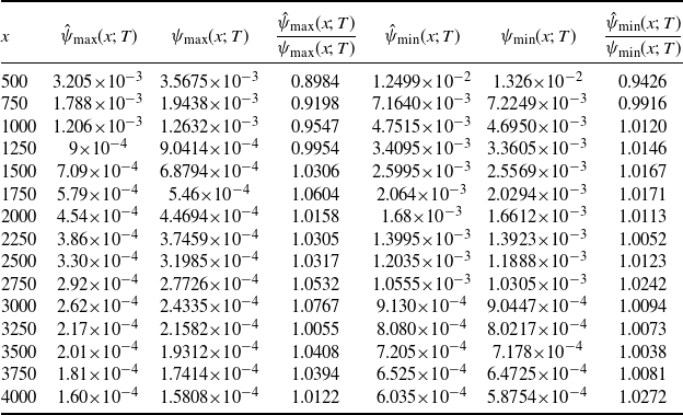
 ψmax(x;T)
 ψmin(x;T)


