2.1. Non-dimensionalisation

We make the model described above non-dimensional by introducing dimensionless variables (denoted by the tilde diacritic):

(2.8a–c)\begin{equation} h = h_\infty \tilde h, \quad x = \frac{\rho g h_\infty^3}{3 \mu U} \tilde x, \quad t = \frac{\rho g h_\infty^3}{3 \mu U^2} \tilde t, \end{equation}

in a manner similar to Perazzo & Gratton (Reference Perazzo and Gratton2008), Lister & Hinton (Reference Lister and Hinton2022) and Taylor-West & Hogg (Reference Taylor-West and Hogg2024). The fluid depth is scaled by the far-field thickness, while the other characteristic scales may be found by balancing the advective flux and the flux associated with gravitational slumping. The time scale is then given by the rate of advection over the horizontal length scale. With this rescaling the governing equations (2.2) may be rewritten as

(2.9a)\begin{equation} \tilde h_{\tilde t} ={-} {\tilde q}_{\tilde x} = \left[ \tilde h + \frac{\tilde Y^2 ( 3 \tilde h - \tilde Y )}{2} \tilde h_{\tilde x} \right]_{\tilde x}, \end{equation}

where

(2.9b)\begin{equation} \tilde Y = \max \left( 0, \tilde h + \frac{Bi}{\tilde h_{\tilde x}} \right). \end{equation}

Here, we have written $| \tilde h_{\tilde x} | = - \tilde h_{\tilde x}$ since all the solutions considered here will have $\tilde h_{\tilde x} \leq 0$. The evolution of the accretionary wedge is now determined solely by a Bingham number

(2.10)\begin{equation} Bi \equiv \frac{\tau_y h_\infty}{3 \mu U}, \end{equation}

which is the ratio of the yield stress to the characteristic viscous shear stress in the system. We also rewrite the boundary, initial and integral conditions, (2.3), (2.5) and (2.7), as

(2.11a)$$\begin{gather} \tilde q ={-} \tilde h - \frac{\tilde Y^2 ( 3 \tilde h - \tilde Y )}{2} \tilde h_{\tilde x} = 0, \quad \text{at} \ \tilde x = 0, \end{gather}$$

(2.11b)$$\begin{gather}\tilde h = 1, \quad \text{at} \ \tilde x = \tilde x_n(\tilde t), \end{gather}$$

(2.11c)$$\begin{gather}\tilde h_{\tilde x} ={-}Bi, \quad \text{at} \ \tilde x = \tilde x_n(\tilde t), \end{gather}$$

(2.11d)$$\begin{gather}\tilde h \rightarrow 1, \quad \text{as}\ \tilde t \rightarrow 0. \end{gather}$$

An additional global mass conservation condition can be derived from (2.11):

(2.12)\begin{equation} \int_0^{\tilde x_n} \tilde h_{\tilde t} \,\mathrm{d} \tilde x = 1. \end{equation}

From considerations described earlier in this section, we change the boundary condition as $x \rightarrow \infty$ to one at $x = \tilde x_n(\tilde t)$, with condition (2.11c) serving to fix the new variable $x_n$. The model equations above are not self-consistent if one sets the initial condition $\tilde h = 1$ at $\tilde t = 0$, since then the whole system is initially unyielded, and the no-flux condition (2.11a) is not satisfied. Thus, we instead modify the original initial condition by initialising the system at some small time $0 < \tilde t \ll 1$ and a corresponding small yielding downsloping wedge satisfying $\tilde h - 1 \ll 1$, $\tilde h_{\tilde x} \leq -Bi$ at $0 \leq \tilde x < \tilde x_n$. In §§ 3, 4, 5.2 and 5.3 we drop the diacritical marks from dimensionless variables for simplicity of notation.

3.1. Numerical methods

Equations (2.9) and (2.11) are solved using a Crank–Nicolson finite difference scheme with a non-uniform grid spacing and adaptive time stepping, using an approach similar to that of Ball et al. (Reference Ball, Penney, Neufeld and Copley2019). The fluid flux, which has both advective and diffusive terms, is discretised using the Il'in method (Il'in Reference Il'in1969; Clauser & Kiesner Reference Clauser and Kiesner1987). The fluid height $h$ is evaluated at the centres of the grid bins, while the flux $q$ is computed at the bin boundaries. The fluid height can then be evolved by using a discrete version of the mass conservation equation $h_t + q_x = 0$. We start time integration from a small parabolic wedge of length $x_n$ that satisfies the boundary conditions (2.11a)–(2.11c). The domain of computation spans a region longer than $x_n$ and uses the boundary condition $h = 1$ at the far end instead of (2.11b) and (2.11c). As the fluid wedge grows, we extend the spatial domain by stretching the mesh and remapping to the new mesh points using linear interpolation. In order to treat the regions with $Y > 0$ and $Y = 0$ in the same manner and make the numerical scheme more well-behaved, we regularise the yield surface height equation (5.2b) using the approximation

(3.1)\begin{equation} Y = \frac{1}{2} \left[ \left( h - \frac{Bi}{|h_x|} + \epsilon_1 \right) + \left( h - \frac{Bi}{|h_x|} - \epsilon_1 \right) \tanh\left( \frac{1}{\epsilon_2} \left\{ h - \frac{Bi}{|h_x|} \right\} \right) \right], \end{equation}

where $\epsilon _1,\ \epsilon _2 \ll 1$. The case $Y = 0$ in (5.2b) is replaced by a small non-zero yield surface height $\epsilon _1$ (Jalaal et al. Reference Jalaal, Stoeber and Balmforth2021), while the tanh function regularises the sharp transition between the cases $h - Bi / | h_x | > 0$ and $h - Bi / | h_x | < 0$. Here we use $\epsilon _1 = \epsilon _2 = 0.001$ after checking that reducing these values has negligible impact on the numerical results. We observed that the results converge as the spatial and temporal steps are reduced and ensured they are small enough for the numerical scheme to be stable.

3.2. Numerical results

The evolution of the computed fluid topography for $Bi = 1$ is shown in figure 2. The solution has a well-defined nose position at which fluid surface transitions almost discontinuously (given the regularisation (3.1)) from sloping to horizontal with height $h = 1$ according to (2.11c). The initial horizontal fluid surface remains undisturbed until the nose of the wedge passes the location. We also see that close to the nose the yield surface becomes nearly vertical.

Figure 2.

Bingham fluid surface height $h$ (black) and yield surface height $Y$ (blue) at $t = 0.021, 0.23, 1.5, 10$ for $Bi = 1$. Darker lines correspond to later times.

In figure 3 we present the evolution of the wedge thickness, length and yield surface height for a range of Bingham numbers. We observe a power-law behaviour in all these quantities at early and late times, suggesting asymptotically self-similar evolution as $t \rightarrow 0\text { and } t \rightarrow \infty$. There is some non-power-law evolution during the very first few time steps (omitted in figure 3), which quickly transitions to power-law behaviour. We derive the corresponding power-law scaling exponents in § 4, where we also show that for low $Bi$ there is an approximate self-similar behaviour at intermediate time values. These theoretically predicted exponents are shown in figure 3 and accurately match the numerical results.

Figure 3.

(a) Evolution of the wedge height (black and grey solid lines) and the yield surface height (blue dashed lines) at the backstop for a Bingham fluid at various $Bi$ values. (b) Evolution of the change in wedge height at the backstop (black and grey solid lines) and the wedge length (red dashed lines) for a Bingham fluid at various $Bi$ values. In both panels, the triangles show analytically predicted asymptotic power-law dependence with the following exponents (derived in § 4): $1/2$ for the early-time regime, $1/4$ and $3/4$ for the late-time regime and $1/3$, $2/3$ and $1/6$ for the very-late-time regime.

Individual fluid surface profiles in figure 4 show a distinct difference in evolution at low and high Bingham numbers. At low $Bi$ the yield surface remains close to the fluid surface for a long time. For example, in the case of $Bi = 0.0032$, this is seen at least until $t = 11\,000$ (figure 4a,b), meaning that the flow is quasi-Newtonian with a thin pseudo-plug layer at the top. Only after the wedge has grown much larger than $h_\infty$ does the yield surface start to grow at a slower rate than the fluid surface (figure 4c) until the yield surface height becomes a small fraction of $h$. This results in a predominantly unyielded, quasi-static wedge. On the other hand, the flow at high Bingham numbers (figure 4d,e) is always quasi-static, as the yielded layer is much thinner than the total fluid thickness. In what follows, we use terms early time and late time to respectively denote the regimes where the maximum fluid thickness increase $h_0-1$ is much less and much greater than 1, where $h_0$ is the fluid thickness at the backstop. In figure 4(b,c) we see two late-time regimes that occur one after another, distinguished by a significant or negligible yield surface height. We call the latter regime the very-late-time regime.

Figure 4.

Examples of numerically obtained states that are close to asymptotic solutions for $n = 1$. Dashed lines show self-similar asymptotic predictions outlined in § 4. (a) $Bi = 0.0032$, $t = 0.014$, corresponding to the early-time quasi-Newtonian regime. The asymptotic prediction for fluid surface is obtained by solving (4.2), which is used in conjunction to (2.9b) to obtain the yield surface. (b) $Bi = 0.0032$, $t = 11\,000$, corresponding to the late-time quasi-Newtonian regime. (c) $Bi = 0.0032$, $t = 7.2 \times 10^{11}$, corresponding to the very-late-time quasi-static regime. (d) $Bi = 40$, $t = 9.0 \times 10^{-5}$, corresponding to the early-time quasi-static regime. The asymptotic predictions are obtained in the same way as for (a). (e) $Bi = 40$, $t = 10$, corresponding to the very-late-time quasi-static regime.

We gain more insight into the self-similar regimes by plotting the numerically fitted power-law exponent, $\alpha$, of $h_0 - 1\sim t^\alpha$ as a function of time and the Bingham number (figure 5a). The exponent is obtained by finding a gradient of $\log (h_0(t) - 1)$ with respect to $\log (t)$ in a narrow time window. The width of this window is kept fixed in $\log (t)$ space as the mean time value is changed. From the description in the last paragraph, the behaviour of the wedge height at the backstop $h_0$ distinguishes the late-time regime from the early-time one. Similarly, the fraction of the wedge thickness taken up by the yielded layer at the backstop $Y_0 / h_0$ is a good descriptor of how quasi-static or quasi-Newtonian the wedge is. Hence, we can use the isolines of $h_0$ and $Y_0/h_0$ (respectively black and red solid lines in figure 5a) to demarcate the boundaries between different regimes. Indeed, we see that the power exponent $\alpha$ tends to change its value close to these lines, indicating a change in self-similar behaviour, while far from the lines the exponent stays the same, meaning that the system is asymptotically close to one of the self-similar states. We also note that at sufficiently late times the system always reaches the quasi-static regime. With increasing $Bi$, this very-late-time quasi-static regime is reached at earlier times, until for $Bi \gtrsim 1$, the quasi-Newtonian regime is not observed at all. The dashed lines show approximate analytical regime boundaries that are derived in § 4. They match the numerically obtained boundaries very well, given the fact that the transitions between the asymptotic regimes are smooth and occur over a large interval of $Bi$ and $t$ values.

Figure 5.

(a) Regime diagram of the model solutions for $n = 1$, showing how the power scaling exponent, $\alpha$, of $h_0 - 1 \sim t^\alpha$, depends on $Bi$ and time. Dashed lines (black, separating the early and late regimes; red, separating quasi-static and quasi-Newtonian regimes) denote analytically predicted boundaries between the regimes, while the solid lines mark the numerically obtained boundaries. Markers correspond to computed states shown in figure 4. White areas are difficult to access numerically and so we were able to do only a limited number of computations there. (b) Analytically obtained regime diagram showing where different self-similar regimes are expected to hold for the Bingham fluid ($n = 1$).

5.1. Herschel–Bulkley fluid model

The model of the Bingham fluid wedge can be generalised by instead considering a Herschel–Bulkley constitutive relation (Frigaard Reference Frigaard2019). This incorporates shear-thinning behaviour which is more applicable to strain localisation in tectonic environments. The dimensional constitutive relation expressed in the lubrication approximation limit is therefore of the form

(5.1)\begin{equation} \frac{\partial u}{\partial z} = \left\{ \begin{array}{@{}ll@{}} 0, & \left| \tau_{xz} \right| \le \tau_y, \\ K^{{-}1/n} \text{sgn} (\tau_{xz}) ( |\tau_{xz}| - \tau_y )^{1/n} , & \left| \tau_{xz} \right| > \tau_y. \end{array} \right. \end{equation}

Here $K$ is the consistency, which determines the magnitude of deformation given the shear stress, and $n$ is the power-law index which describes the extent to which the fluid is shear thinning. In this study we assume that $n \in (0,1]$. For $n = 1$ the Herschel–Bulkley relationship recovers the Bingham relationship with $K = \mu$. Conversely, as $n \rightarrow 0$, the fluid becomes more shear thinning, with the $n \rightarrow 0$ case corresponding to a perfectly plastic material.

The flux associated with the shear of a Herschel–Bulkley fluid was derived by Balmforth et al. (Reference Balmforth, Craster, Rust and Sassi2006), while Taylor-West (Reference Taylor-West2023) derived a set of non-dimensional governing equations for the Herschel–Bulkley fluid that are analogous to (2.9) and (2.11) and describe the evolution of the wedge height and the yield surface. In the notation used here, the Herschel–Bulkley wedge is determined by

(5.2a)$$\begin{gather} \tilde h_{\tilde t} ={-} \tilde q_{\tilde x} = \left[ \tilde h + Bi^{1/n-1} \frac{\tilde Y^{1/n+1} ( (2n+1) \tilde h - n \tilde Y )}{(n+1) ( \tilde h - \tilde Y )^{1/n-1}} \tilde h_{\tilde x} \right]_{\tilde x}, \end{gather}$$

(5.2b)$$\begin{gather}\tilde Y = \max \left( 0, \tilde h - \frac{Bi}{ \left| \tilde h_{\tilde x} \right|} \right). \end{gather}$$

The flux condition at the origin, the nose conditions and the initial condition are respectively described by

(5.3a)$$\begin{gather} \tilde q ={-} \tilde h - Bi^{1/n-1} \frac{\tilde Y^{1/n+1} ( (2n+1) \tilde h - n \tilde Y )}{(n+1) ( \tilde h - \tilde Y )^{1/n-1}} \tilde h_{\tilde x} = 0, \quad \text{at} \ \tilde x = 0, \end{gather}$$

(5.3b)$$\begin{gather}\tilde h = 1, \quad \text{at} \ \tilde x = \tilde x_n, \end{gather}$$

(5.3c)$$\begin{gather}\tilde h_{\tilde x} ={-}Bi, \quad \text{at} \ \tilde x = \tilde x_n, \end{gather}$$

(5.3d)$$\begin{gather}\tilde h \rightarrow 1, \quad \text{as}\ \tilde t \rightarrow 0. \end{gather}$$

The statement of conservation of global mass can be derived from (5.3), and may be written as

(5.4)\begin{equation} \int_0^{\tilde x_n} \tilde h_{\tilde t} \,\mathrm{d} \tilde x = 1. \end{equation}

Here

(5.5)\begin{equation} Bi \equiv \left[ \frac{n h_\infty}{(2 n + 1) U} \right]^n \frac{\tau_y}{K} \end{equation}

is the equivalent Bingham number for a Herschel–Bulkley fluid. The corresponding non-dimensionalisation scales are equivalently

(5.6)\begin{equation} h = h_\infty \tilde h, \quad x = \left[ \frac{n}{(2 n + 1) U} \right]^n \frac{\rho g h_\infty^{n+2}}{K} \tilde x, \quad t = \left[ \frac{n}{(2 n + 1) U} \right]^n \frac{\rho g h_\infty^{n+2}}{K U} \tilde t. \end{equation}

5.2. Asymptotic regimes

A study of self-similar regimes can similarly be undertaken for the Herschel–Bulkley fluid model described by (5.2) and (5.3). This results in the change of some of the power-law exponents and prefactors, but the nature of the regimes and their qualitative position in the $Bi$–$t$ space remain unchanged. Hence, below we only state the key results for the Herschel–Bulkley rheology that differ from the Bingham model. The behaviour corresponding to the quasi-Newtonian regime in the case of $n = 1$ is called the quasi-power-law regime in the case of $n < 1$.

The early-time power-law dependence for height and length remain $h - 1 \sim t^{1/2}$ and $x_n \sim t^{1/2}$. However, the early quasi-power-law wedge takes a different shape than for $n = 1$. On the other hand, the shape of the early quasi-static wedge is unaffected by varying power law index $n$ and stays linear, since it is determined by the quasi-static condition $Y \simeq 0$ that remains the same for the Herschel–Bulkley fluid. The yield surface height in this regime generalises to

(5.7)\begin{equation} Y(x, t) = \left[ \left( \frac{1 + n}{1 + 2n} \right)^n \left( 2 Bi^{{-}1} (x_n - x) \right)^{1/2} \right]^{1/(1 + n)}, \end{equation}

assuming $Y \ll n$.

The shape of the fluid surface in the late-time quasi-Newtonian regime is governed by the balance of advective and diffusive fluxes, so that in the case of general Herschel–Bulkley rheology the corresponding quasi-power-law solution is different from that for $n = 1$:

(5.8a)$$\begin{gather} h(x, t) = [(2+n) (x_n - x)]^{1/(2+n)}, \end{gather}$$

(5.8b)$$\begin{gather}x_n = \frac{\left[ (3 + n) t \right]^{(2+n)/(3+n)}}{2 + n}. \end{gather}$$

Gratton & Perazzo (Reference Gratton and Perazzo2009) studied a similar model a using power-law viscous rheology and obtained solutions that match (5.8) for the quasi-power-law regimes of our model.

The late quasi-static regime, in a manner similar to the early quasi-static regime, exhibits only a yield surface shape that is different for the Herschel–Bulkley rheology:

(5.9)\begin{equation} Y = \left[ \left( \frac{n+1}{2n+1} \right)^n Bi^{{-}1/(2 n)} (2 (x_n - x))^{1/2} \right]^{1/(1+n)}. \end{equation}

In terms of the regime location in the $Bi$–$t$ space (figure 5b), only the boundary between the late quasi-power-law and the late quasi-static regime shifts from $t \sim Bi^{-4}$ to ${t \sim Bi^{-(1 + 3/n)}}$. In other words, for this specific non-dimensionalisation, a shear-thinning wedge spends more time being quasi-power-law before becoming quasi-static.

5.3. Numerical results

Figure 6 compares the numerically computed state of the system for Bingham ($n = 1$) and shear-thinning Herschel–Bulkley ($n = 0.386$) rheologies. Since the rheological power exponent affects the fluid velocity and thus the flux for a given wedge geometry, the yield surface shape is seen to be different for different $n$ values. In the case where the fluid flow is quasi-static (figure 6d,e), the shape of the fluid surface is governed by the yielding surface in (5.2b) being close to the base, which does not depend on $n$. As a result, figure 6(c–e) shows surface shapes insensitive to $n$. On the other hand, when most of the fluid layer is yielded, the wedge topography depends heavily on $n$, as discussed earlier in this subsection. In figure 6(a) we observe that for low $Bi$ the shear-thinning wedge is shorter and has a much steeper yield surface than the Bingham wedge. This difference in wedge aspect ratio carries on into the late quasi-power-law regime (figure 6b), with the shear-thinning wedge being shorter, which is a consequence of the $x_n (t)$ time power exponent in (5.8a) being lower for lower $n$ in (5.8b). The last important difference in the system with the shear-thinning rheology is that for low $Bi$ it reaches the very-late-time regime at much later times than the system with $n = 1$. This is clearly seen in figure 6(c), where the Bingham wedge is already close to the very-late-time quasi-static regime, while the shear-thinning wedge is still quasi-power-law, with little separation between the yield surface and the fluid surface. Indeed, for $n = 0.386$ and $Bi = 0.0032$, we would expect for the transition time to be ${\sim }Bi^{-(1 + 3/n)} \sim 10^{22}$, which we cannot readily access numerically.

Figure 6.

Fluid surfaces (in black) and yield surfaces (in blue) compared for $n = 1$ (solid lines) and $n = 0.386$ (dashed lines): (a–c) $Bi = 0.0032$ and times $0.22, 2.6 \times 10^4 \text { and } 6.3 \times 10^{9}$, respectively; (d,e) $Bi = 40$ and times $0.0011$ and $14$, respectively.

6.1. Experimental methods

To examine the behaviour of a physical fluid wedge we conduct a series of experiments using a commonly available viscoplastic fluid. We used ultrasound gel (Anagel^{^{TM}}) as the experimental fluid because it is commercially available in large quantities and has a similar composition to Carbopol, which is commonly used for yield-stress fluid experiments. As described in the next subsection, the gel can be accurately described by a Herschel–Bulkley constitutive relation. In order to remove bubbles, the gel was mixed in 3 litre beakers for about two hours by incrementally raising the mixing head from the bottom of the beaker to its top.

We reproduce the geometry of our model in a square tank with a movable vertical backstop, as shown in figure 7. The tank has a length of $150\,\text {cm}$, width of $20\,\text {cm}$ and height of $20\,\text {cm}$ and is made of acrylic glass. A computer-controlled stepper motor can move the backstop at a fixed speed $0.10\,\text {mm}\,\text {s}^{-1} \leq U \leq 6.00\,\text {mm}\,\text {s}^{-1}$. The gap between the backstop and the base is small enough for the leakage to be negligible. At the opposite end of the tank there is a plate that is set at the height of the initial fluid layer. To ensure that the gel does not slip with respect to the base of the tank, we covered the base with 60 grit waterproof aluminium oxide sandpaper. We verified that there is no slip by slowly inclining a sandpaper-covered plate with a lump of gel on top and observing that the upstream contact line did not move after the gel started flowing (Maillard et al. Reference Maillard, Mézière, Moucheront, Courrier and Coussot2016). Instead of sliding, we observed slumping-like flow with the contact area between the base and the fluid not changing. During the experiments we used a green line laser to illuminate a sheet of the gel of around $1.5\,\text {mm}$ in thickness. The laser light was let through a narrow 5 mm width slit cut along the centreline of the sandpaper base.

Figure 7.

A schematic diagram of the experimental set-up.

Experiments were done by filling the tank with a uniform layer of gel of thickness $h_\infty$ and moving the backstop at a fixed speed $U$. The system was imaged every 2–4 s by a Nikon digital SLR camera D7000, allowing us to extract the fluid surface shape over time. We placed the camera far enough from the tank for the distortion of images to be negligible.

6.2. Rheometry

Since ultrasound gel is not a commonly used experimental material, we did a rheological study to determine its constitutive relation. Haist et al. (Reference Haist2020) have looked into various ways to measure the rheology of ultrasound gel and fitted a Bingham constitutive relation. However, they found that their results depend quite heavily on the measurement set-up.

Rheological measurements were done using a Kinexus Pro+ rheometer by NETZSCH with a parallel-plate geometry. Rough plates were used to reduce the potential for slip. The diameter of the plates was $40\,\text {mm}$, and a gap of $1\,\text {mm}$ was kept in all of the measurements. We conducted decreasing shear strain-rate ramps, following a procedure similar to that in Dinkgreve et al. (Reference Dinkgreve, Paredes, Denn and Bonn2016). Initially, the gel was pre-sheared at $100\,\text {s}^{-1}$ for $30\,\text {s}$ and then left to rest for $30\,\text {s}$ to ensure that all the tests started with the same initial shear state. Immediately afterwards, a logarithmic shear rate ramp lasting for $2\,\text {min}\ 40\, \text {s}$ was imposed from $100\,\text {s}^{-1}$ down to $10^{-5}\,\text {s}^{-1}$. We checked that making the ramp last longer did not affect the results, meaning that the ramp is slow enough for the gel to be in a quasi-steady shear state. Running the shear rate ramp in reverse showed little thixotropy. Using parallel plates results in a spatially varying stress field during the measurement, which we take into account by applying the Weissenberg–Rabinowitsch correction (Rabinowitsch Reference Rabinowitsch1929; Mendes, Alicke & Thompson Reference Mendes, Alicke and Thompson2014) in a similar manner to Varges et al. (Reference Varges, Costa, Fonseca, Naccache and Mendes2019) and Haist et al. (Reference Haist2020). All values of shear rate and stress are assessed at the rim of the rheometer plates.

The results of three such shear ramps are presented in figure 8. The measured stress–strain-rate curve is found to be less reproducible for different gel samples at shear rates below around $1\,\text {s}^{-1}$, even though the samples were taken from the same location in the bulk of the gel. However, the results above ${\sim }1\,\text {s}^{-1}$ have very low variability and match the Herschel–Bulkley model very well. The discrepancy at low shear rates is likely due to wall slip in the rheometer (Magnin & Piau Reference Magnin and Piau1990; Barnes Reference Barnes1995; Mendes et al. Reference Mendes, Alicke and Thompson2014) since we observe that the apparent yield stress at low shear rates decreases with decreasing plate gap thickness.

Figure 8.

Decreasing shear-rate ramp measurement results for three different samples taken from the same gel pack. At low shear rates (grey area) the different samples give rather different stresses, which we hypothesise is due to wall slip. Herschel–Bulkley model fit (red line) at high shear rates (white area) is consistent for different samples. The variable values are given at the rim of the rheometer plates.

We obtain the Herschel–Bulkley parameters by fitting this model to an increasing number of data points, starting from the highest shear rate. We minimise the total error in the fitting parameters,

(6.1)\begin{equation} \Delta = \sqrt{\left( \frac{\Delta n}{n} \right)^2 + \left( \frac{\Delta \tau_y}{\tau_y} \right)^2 + \left( \frac{\delta K}{K} \right)^2}, \end{equation}

with respect to the number of data points used for the fit and use the corresponding number of data points to get the best estimate of $\tau _y$, $n$ and $K$. Figure 8 shows an example of a fit (red line) obtained by this method.

We repeated shear-rate ramp measurements for different gel samples taken from the same source in order to estimate the random uncertainty in the measured rheological parameters. The resultant uncertainties of the rheological parameters are presented in table 2. They were found to be dominant over the uncertainty associated with the high-$\dot \gamma$ misfit of the Herschel–Bulkley model. We also checked that the gel temperature has a negligible effect on the measurement results in a temperature range of $17.5\unicode{x2013}25.0\,^{\circ }\text {C}$.

Table 2.

Experimental parameters and associated uncertainties.

6.3. Experimental results

In total 13 experiments were conducted, as summarised in table 2. We varied the initial layer thickness $h_\infty$ and the scraping speed $U$ and measured the gel rheology after every experimental session. Low-$h_\infty$ experiments (1–3, 7, 8) allow us to reach larger dimensionless times, but result in a steeper fluid surface slope (0.35 on average) and hence a larger anticipated deviation away from the lubrication approximation. On the other hand, experiments with larger $h_\infty$ have a lower gel surface slope of around 0.16 and provide more data points in the early-time regime. With our set-up and ultrasound gel as the experimental fluid it is impossible to explore the dynamics associated with low Bingham numbers, which makes the quasi-power-law regimes inaccessible.

Experiments done by Taylor-West & Hogg (Reference Taylor-West and Hogg2024) were similar but had a few important differences. They used hair gel as an experimental fluid. Although its main ingredient (Carbopol) is the same as in ultrasound gel, hair gel has a lower yield stress and a higher consistency, thereby making it more difficult to achieve higher $Bi$. Also, their experiments did not try to eliminate basal slip but instead took it into account by considering a slip law with carefully chosen parameters. Nevertheless, such basal slip is often one of the key sources of experimental uncertainty.

Figure 9(a) shows a characteristic image of the illuminated fluid wedge during an experiment, while figures 9(b) and 9(c) show pictures of the wedge at the end of experiments 1 and 13, respectively. An image sequence of a full experiment is shown in movie 1 available at https://doi.org/10.1017/jfm.2024.908. These images were used to measure the fluid surface height by detecting where a green channel intensity value exceeded a chosen threshold intensity. When devising the detection algorithm, we also took into account occasional bright reflections, brightly illuminated bubbles, shadows in gel illumination and longitudinal variations in illumination intensity, some of which can be seen in figure 9(a). The wedge nose position $x_n$ is defined experimentally as the horizontal coordinate where the fluid surface height falls below a predefined threshold. For nose positions we therefore measured the initial horizontal surface shape, obtaining its mean height $h_\infty$ with an associated standard deviation. Then we chose the height threshold for $x_n$ to be two standard deviations above the mean initial height. On average, this threshold $\Delta h_{th}$ was found to be $1.6$ mm or $7\,\%$ above the initial gel surface height.

Figure 9.

(a) A single experimental image with laser illumination; $h_{\infty } = 3.85\,{\rm cm}$, $U = 0.5\,{\rm mm}\,{\rm s}^{-1}$ (exp. 11). Brightness and contrast enhanced. (b) Photograph of the gel wedge immediately after experiment with $h_\infty = 1.00\,{\rm cm}$, $U = 0.5\,{\rm mm}\,{\rm s}^{-1}$ (exp. 1). Creases are clearly visible. Transverse variation in fluid surface height is noticeable. (c) Photograph of the gel wedge immediately after experiment with $h_\infty = 3.90\,{\rm cm}$, $U = 2.0\,{\rm mm}\,{\rm s}^{-1}$ (exp. 13). The flow is closer to a quasi-two-dimensional one than in experiment 1.

The dominant sources of experimental uncertainty are in the measurements of $x_n$ and $h_\infty$ (table 2). The uncertainty in the wedge nose position is due to the fact that the predicted nose discontinuity in the fluid surface slope is smoothed out in the experiments, requiring us to use the threshold $\Delta h_{th} \approx 0.07 h_\infty$ as described in the previous paragraph. The arbitrariness of this threshold sets the uncertainty in dimensional $x_n$, and we estimate it to be

(6.2)\begin{equation} \Delta x_n = 0.5 \frac{\Delta h_{th}}{\left| h_x (x_n^-) \right|} = \frac{\Delta h_{th} \rho g h_\infty}{2 \tau_y}, \end{equation}

where we used (2.7) as an estimate for the slope at the nose. We also note that at late times the experiments exhibit a boundary layer close to the backstop. This introduces an uncertainty of around $5\,\%$ in the experimental determination of the dimensional $h_0$ when comparing it with the modelled surface height at the backstop, as it is not clear where the height needs to be measured to best represent the theoretical (dimensional) $h_0$.

Two sets of measured gel surface profiles in the frame of the moving backstop are shown in figure 10(a) for a lower $h_\infty$ experiment and figure 10(b) for higher $h_\infty$ (note the truncated vertical axis). We observe that the wedge length and height grow monotonically with time. As seen from the decreasing spacing between surface profiles, the growth of the wedge height slows down with time. The fluid surface slope at the measured nose position is generally lower than that predicted by the thin-layer model, as shown by the blue lines. This was similarly reported by Taylor-West & Hogg (Reference Taylor-West and Hogg2024). However, the observed slope increases quite rapidly just above the nose of the wedge, reaching values similar to those predicted. Irrespective of the experimental parameter values, crease-like features formed in the gel surface as the wedge was growing, which were also observed by Maillard et al. (Reference Maillard, Mézière, Moucheront, Courrier and Coussot2016).

Figure 10.

(a) Measured fluid surface profiles (black) for $h_\infty = 0.95\,{\rm cm}$, $U = 4.0\,{\rm mm}\,{\rm s}^{-1}$ (exp. 8). The surface is plotted every $7\,\text {s}$. (b) Measured fluid surface profiles for $h_\infty = 3.90\,{\rm cm}$, $U = 2.0\,{\rm mm}\,{\rm s}^{-1}$ (exp. 13). The surface is plotted every $14\,\text {s}$. Note that the vertical axis starts from a non-zero value. Blue lines indicate surface slope at the wedge nose as predicted by (2.7). The aspect ratio in both plots is exaggerated. The profiles are truncated at the measured nose position or at the edge of the imaging area.

As shown in figure 11, the dimensionless experimental wedge height and length measurements have a reasonably good agreement with the model predictions. The results are plotted versus $Bi\ \tilde t$, because $\tilde t \sim Bi^{-1}$ corresponds to the predicted transition between the early- and the late-time regimes. Experiments run at different $U$ and $h_\infty$ are combined together, with red and blue markers indicating the low- and high-$h_\infty$ experiments, respectively, while the black lines show the model predictions. Because the predictions depend weakly on the Bingham number, we only plot them for the smallest and largest $Bi$ value achieved in the experiments. The scatter of points within the two groups of experiments is rather weak, indicating that experiments are quite reproducible even when the scraping speed $U$ is varied. The maximum wedge height in all of the experiments (figure 11a) has a better match with the model predictions at later times than at the start. In particular, the wedge height in the high-$h_\infty$ experiments is ${\approx }12\,\%$ lower than predicted, which is not explained by the uncertainty in the $\tilde{h}_0$ measurement. The heights for small $h_\infty$ at earlier times are also too low, which is likely due to uncertainty in the $\tilde h_0$ measurement as indicated by the cyan error bars. Towards the end of the experiments, the wedge height is of the predicted size, but also increases at a faster rate than predicted. The experimentally observed wedge length matches the model predictions for a wide range of time values (figure 11b) and shows a universal trend irrespective of the experimental parameters. The early-time length may be slightly above the theoretical predictions, but is within the range of the experimental uncertainty.

Figure 11.

Experimental results of the dimensionless (a) wedge height $\tilde h_0$ (height change $\tilde h_0 - 1$ in the inset) and (b) length for all the experiments compared with the model predictions at $n = 0.37$ and $Bi = 1.84, 8.16$ (black lines). Blue points denote higher-$h_\infty$ experiments, while red points mark the lower-$h_\infty$ experiments. The horizontal axis shows dimensionless time $\tilde t$ multiplied by $Bi$, because $Bi\ \tilde t \approx 1$ is when the transition from early to late times is expected to happen. Cyan and magenta error bars denote uncertainty for the lower- and higher-$h_\infty$ experiments, respectively. The uncertainty in $Bi\ \tilde{t}$ is of the order of the marker size.

In figure 12 we show rescaled fluid surface profiles according to the modelled universal self-similar profiles for experiments 1 and 12. The profiles appear to collapse to a universal shape for both late times (figure 12a,b) and the early times (figure 12c). For the early-time profiles of the high thickness experiment we do see a linear trend as predicted, but the surface slope corresponds to a Bingham number that is approximately half of the measured one. Surface profiles of other experiments (not shown here) have a similar linear shape at early times but also behave as if the Bingham number was lower. The predicted late-time shape is matched very well for small-$h_\infty$ experiments (figure 12a), and a similar behaviour is seen in other small-$h_\infty$ experiments. The large-$h_\infty$ experiments (figure 12b) did not reach late enough times for the late-time asymptotic regime, but they match well the computed intermediate shape (dashed line).

Figure 12.

Experimental profiles of the gel surface scaled to the predicted universal self-similar shapes. (a) $h_\infty = 1.00\,{\rm cm}$, $U = 0.5\,{\rm mm}\,{\rm s}^{-1}$ (exp. 1) for the late-time regime. Surface profiles are plotted every 40 s and get darker with increasing time. Dashed line indicates the asymptotic self-similar shape (row 4 of table 1). (b) $h_\infty = 3.85\,{\rm cm}$, $U = 0.5\,{\rm mm}\,{\rm s}^{-1}$ (exp. 12) for the late-time regime. Surface profiles are plotted every 20 s and get darker with increasing time. Dashed line indicates theoretically predicted surface shape at the end of the experiment. (c) $h_\infty = 3.85\,{\rm cm}$, $U = 0.5\,{\rm mm}\,{\rm s}^{-1}$ (exp. 12) for the early-time regime. Surface profiles are plotted every 8 s and get darker with decreasing time. Only the first few profiles are shown. Dashed line shows the early-time asymptotic self-similar prediction (row 2 of table 1) at $Bi$ value that best fits the experimental data.

The experimental wedge has some features that are not taken into account by our model. The wedge surface has prominent creases (figure 9b) that have smooth crests but very sharp troughs where the fluid surface slope is seemingly discontinuous. The creases formed in all experiments. In both images in figures 9(b) and 9(c) the surface shape is quasi-two-dimensional, as assumed in our model. However, there is also some three-dimensionality caused by sidewall shear. Specifically, close to the backstop the gel thickness is lower at the centre than near the sidewalls, while close to the wedge nose the central thickness is higher than at the sidewalls. This effect is more prominent in the low-$h_\infty$ experiments and may result in a lower measured surface slope at the central plane. We also see that the wedge has a rather steep slope, which might make the lubrication approximation less reliable.

Another feature that is not accounted for in our theory is the positive fluid surface slope next to the backstop. As observed by Taylor-West & Hogg (Reference Taylor-West and Hogg2024), this is a consequence of limited slip with respect to the backstop resulting in a boundary layer at $x = O(h)$ where the lubrication approximation breaks down. Our experimental profiles in figure 10(b) indeed show that the width of this boundary layer with positive slope increases approximately linearly with the wedge height. Other experiments have the boundary layer contaminated by the creases or the whole of it being too close to the backstop to measure, which makes it difficult to draw more quantitative conclusions.

Here we examine some preliminary particle image velocimetry (PIV) results to better understand the deformation of the experimental wedge. Figure 13 shows a snapshot of an experiment at $U = 7\,{\rm mm}\,{\rm s}^{-1}$ and $h_\infty = 1.30\,\text {cm}$. 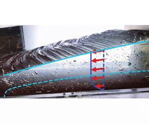This experiment differs from those studied in § 6 because there is no sandpaper on the tank base and the surface slope is much steeper due to fast scraping speed $U$. However, the measured fluid velocity is still predominantly horizontal and some key features of the wedge dynamics are uncovered by plotting the fluid velocity magnitude. The top part of the wedge (in white) is effectively unyielded and moves together with the backstop, while the horizontal layer beyond the nose of the wedge (in black) forms another slowly deforming region that is at rest in the laboratory frame. This is very similar to the scraping experiments of Maillard et al. (Reference Maillard, Mézière, Moucheront, Courrier and Coussot2016) in a very similar geometry but with a small gap between the base and the backstop. A yield surface separates the top pseudo-plug from the deforming layer below, as predicted by the simple thin-layer model. However, the model fails close to the nose of the wedge where the yield surface intersects the surface of the fluid. As seen from the steep gradient in $|\boldsymbol {u}|$, the nose of the wedge is the most rapidly deforming part of the fluid surface, indicating that the creases likely form one at a time close to the nose of the wedge and then get advected into the pseudo-plug at the upper part of the wedge. Surface crease formation requires relatively high strain rates somewhere in the fluid surface and indicates that there are likely important compressional stresses not accounted for in the present lubrication analysis. These stresses lead to a localised area of high strain rate at the nose of the wedge which results in the periodic creasing and deformation of the surface. As a result, there must be a part of the fluid surface that does not belong to the pseudo-plug and hence the yield surface must at some point cross the fluid surface. We therefore predict that even in an experiment with a shallower fluid surface and no basal slip the qualitative features of figure 13 will remain.

Figure 13.

Magnitude of the fluid velocity with respect to the base at $h_\infty = 1.30\,\text {cm}$, $U = 7\,{\rm mm}\,{\rm s}^{-1}$ and $t = 40.5\,\text {s}$ in an experimental set-up without sandpaper base.