





Impact Statement
Dust storms are natural laboratories for particle-laden turbulence at Reynolds numbers far beyond those of most laboratory facilities. This study develops and validates a wall-modelled large-eddy simulation framework that links energetic turbulent motions, PM10 dust suspension and the electric field in the atmospheric surface layer. The work advances fundamental flow physics by showing how coherent turbulent structures, gravitational settling and electrically induced drift can be treated in a unified model to explain the coupled evolution of airflow, PM10 dust concentration and electric fields. Its broader impact lies in providing a tested computational tool for conditions that are difficult to reproduce or sample fully in the field. Such a tool can support improved interpretation of dust storm observations, assessment of near-surface dust loading and electrically induced hazards and development of more reliable models for air quality, transport safety, infrastructure protection and planetary dust environments, including Mars exploration and hazard mitigation strategies.
1. Introduction
Dust storms are major natural hazards that occur frequently in arid and semi-arid regions. They severely affect human activities, public health and transport safety, and also influence regional and global climate by modifying atmospheric aerosol loading, radiative budgets, cloud microphysics and biogeochemical cycles (Prospero et al. Reference Prospero, Ginoux, Torres, Nicholson and Gill2002; Zheng Reference Zheng2009; Kok et al. Reference Kok, Parteli, Michaels and Bou Karam2012). From a fluid-mechanical viewpoint, a dust storm may be regarded as a high-Reynolds-number particle-laden wall-bounded turbulent flow over an erodible surface, in which the turbulent airflow, near-surface saltating sand grains and suspended dust particles form a complex gas–solid two-phase system (Bagnold Reference Bagnold1941; Shao & Lu Reference Shao and Lu2000; Balachandar & Eaton Reference Balachandar and Eaton2010; Kok et al. Reference Kok, Parteli, Michaels and Bou Karam2012; Brandt & Coletti Reference Brandt and Coletti2022). Field observations show that, during severe dust storms, the friction Reynolds number in the atmospheric surface layer (ASL) can reach
 $O(10^6)$
, which is much larger than that attained in most laboratory wall-bounded turbulent flows. The flow therefore contains not only bursting events, sweeps and ejections, but also large-scale and very-large-scale coherent motions (Townsend Reference Townsend1956; Hutchins & Marusic Reference Hutchins and Marusic2007; Smits et al. Reference Smits, McKeon and Marusic2011).
Dust and sand particles in such flows have a broad size distribution, and their motion involves entrainment, saltation, collision, rebound, splash, suspension, gravitational settling and turbulent diffusion. These processes are accompanied by complex particle–particle, particle–wall and particle–turbulence interactions (Maxey & Riley Reference Maxey and Riley1983; Elghobashi Reference Elghobashi1994; Zheng Reference Zheng2009; Kok et al. Reference Kok, Parteli, Michaels and Bou Karam2012). Coherent structures in the ASL, especially ejection and sweep events as well as large-scale and very-large-scale motions, have been shown to play an important role in dust emission, vertical transport and spatial clustering. Conversely, high particle concentrations near the surface can modulate the mean velocity, turbulence intensity, Reynolds shear stress and coherent structures through momentum exchange, inertial lag and preferential concentration (Squires & Eaton Reference Squires and Eaton1991; Eaton & Fessler Reference Eaton and Fessler1994; Berk & Coletti Reference Berk and Coletti2020). Dust storms therefore provide not only a key system for understanding the initiation, development, maintenance and long-range transport of mineral dust, but also a natural high-Reynolds-number laboratory for studying particle–turbulence interactions, multiscale energy transfer and two-phase feedback in wall-bounded turbulence.
Particle electrification and the resulting electric field are ubiquitous features of dust storms. Early observations showed that the near-surface electric field can be strongly enhanced during dust storms, and may even reverse direction relative to the fair-weather atmospheric electric field (Rudge Reference Rudge1913). Subsequent field measurements further demonstrated that, during severe dust storms, the near-surface electric field strength can reach
 $\sim 200\,{\mathrm{kV\,m}^{-1}}$
, about three orders of magnitude larger than that under fair-weather conditions (e.g. Stow Reference Stow1969; Schmidt et al. Reference Schmidt, Schmidt and Dent1998; Zheng et al. Reference Zheng, Huang and Zhou2003; Zhang & Zhou Reference Zhang and Zhou2020, Reference Zhang and Zhou2023a; Zhang et al. Reference Zhang, Tan and Zheng2023b; Zheng & Liu Reference Zheng and Liu2026).
From a physical viewpoint, particles of different sizes acquire different charge polarities through contact electrification and exhibit different inertial responses and transport pathways. Their spatial separation by turbulent coherent structures produces complex distributions of space-charge density and electric field. Recent studies based on simultaneous multipoint and multifield measurements at the Qingtu Lake Observation Array (QLOA) have shown that the space-charge density in dust storms does not simply form a vertically stratified structure with negative charge aloft and positive charge near the surface. Instead, alternating positive and negative charge regions occur in three-dimensional space, with characteristic scales comparable to the boundary-layer thickness (Zhang & Zhou Reference Zhang and Zhou2020). Consequently, the electric field can reverse direction at different heights and spatial locations. These observations suggest that the electric field is not a quasi-static mean field controlled solely by gravitational settling, but a multiscale stochastic field generated by the combined effects of turbulent coherent structures, size segregation and the differential transport of charged particles.
Spectral and wavelet analyses further show that the wind velocity, PM10 dust (diameter
 $\leq 10$
 $\unicode {x03BC}$
m) concentration and electric field can all exhibit an approximate
 $-5/3$
power-law range at intermediate wavenumbers, although the extent of this range and the strength of small-scale intermittency differ among the three fields (Zhang & Zhou Reference Zhang and Zhou2023
a; Zhang et al. Reference Zhang, Tan and Zheng2023
b; Zhang & Zheng Reference Zhang and Zheng2025). This behaviour reflects the complex coupling among turbulent transport, particle transport, space-charge separation and the non-local response of the electric field. Moreover, the electric force acting on dust particles can be comparable to gravity (Schmidt et al. Reference Schmidt, Schmidt and Dent1998; Zheng et al. Reference Zheng, Huang and Zhou2003), implying that the electric field can directly affect the threshold for particle entrainment (Kok & Renno Reference Kok and Renno2006). For saltating particles, the electric field can also alter their saltation height, flight time, impact velocity and impact angle, thereby affecting splash emission, the near-surface particle concentration and the horizontal and vertical mass fluxes. Previous studies have shown that sand electrification can increase the near-surface concentration of saltating particles, keep particle trajectories closer to the surface and, under certain conditions, reduce the critical friction velocity for aeolian entrainment (Zheng et al. Reference Zheng, Huang and Zhou2003; Kok & Renno Reference Kok and Renno2008). The electric field is therefore not merely a passive by-product of dust storms, but can participate actively in their initiation, maintenance and development through electrification, charge separation, electric forces and particle-transport feedback.
Studies of dust storms, especially those involving the coupling of the wind, particle and electric fields, still rely mainly on field observations. However, field conditions are difficult to control, making it challenging to obtain large sets of repeatable and comparable benchmark data. Existing measurements are also usually restricted to time series at a limited number of heights and spatial locations within the ASL, with limited spatial resolution and coverage. Spatial information inferred from such time series commonly relies on Taylor’s frozen-turbulence hypothesis, which may introduce errors at large scales and low wavenumbers (Guala et al. Reference Guala, Hommema and Adrian2006). Thus, although field observations have revealed important statistical features of wind velocity, dust concentration and electric field within the lowest several tens of metres, they are still insufficient to fully characterise the multiscale dynamics of particle transport, charge separation and electric field evolution in the three-dimensional structure of dust storms.
Numerical simulation has therefore become an important tool for investigating the multifield coupling mechanisms of dust storms. Since the friction Reynolds number of real dust storm flows can reach
 $O(10^6)$
, direct numerical simulation (DNS) is not feasible, and large-eddy simulation provides a more practical approach. To date, only Rahman and co-workers have performed large-eddy simulations of multiphysics processes in dust storms. Rahman et al. (Reference Rahman, Cheng and Samtaney2021) developed a numerical framework coupling atmospheric boundary-layer turbulence, charged-particle transport and electric field solution. In their model, the main body of a dust storm was approximated as a statistically stationary turbulent atmospheric boundary layer. The flow was solved using wall-modelled large-eddy simulation (WMLES), suspended charged particles were described using an Eulerian approach combined with the direct quadrature method of moments, and the electric potential and electric field induced by the space-charge density were obtained by solving Poisson’s equation. The model assumes that particle collisions and charge exchange occur mainly within a very thin near-surface layer, while collisions in the suspended layer are negligible. The suspended particle phase can therefore be treated as a dilute particulate flow with one-way fluid–particle coupling. Rahman et al. (Reference Rahman, Saieed and Hickey2023) subsequently extended this framework to Martian dust storms and used WMLES to compare charge separation and local discharge in charged particle-laden boundary layers on Earth and Mars. Although the models developed by Rahman and co-workers have provided valuable insights, they have not yet been systematically validated against multifield measurements in the ASL. Their ability to quantitatively describe the coupled multiphysics processes of dust storms in the surface layer therefore remains limited.
In this study, we develop a WMLES framework for the coupled multiphysics processes in dust storms at a friction Reynolds number of
 $O(10^6)$
. In the present model, the suspended dust phase is represented by an advection–diffusion–settling equation for the dust concentration field, rather than by the direct quadrature method of moments used in previous studies (Rahman et al. Reference Rahman, Cheng and Samtaney2021, Reference Rahman, Saieed and Hickey2023). To assess the model, the simulated wind velocity, PM10 dust concentration and electric field are compared with measurements at 11 heights in the ASL from the QLOA. The remainder of the paper is organised as follows. Section 2 presents the mathematical formulation of the numerical model. Section 3 compares the model predictions with the QLOA measurements. Section 4 summarises the main conclusions and gives a brief outlook.
2. Model formulation
In this study, we focus on the interaction between suspended PM10 dust particles and turbulent airflow, and therefore neglect near-bed sand saltation within the lowest tens of centimetres above the surface. The flow considered is a near-neutral, fully developed and statistically stationary dust-laden atmospheric boundary layer. To describe the coupled wind–dust–electric processes in dust storms, the model accounts for the interactions among three key physical processes: (1) the evolution of atmospheric boundary-layer turbulence, (2) the release of PM10 dust particles from the surface and their subsequent advection, diffusion and gravitational settling in the turbulent airflow and (3) the electric field generated by charged dust particles and the associated electrically induced particle migration.
In the present study, the coupled system is formulated within a WMLES framework. The carrier airflow is governed by the spatially filtered incompressible Navier–Stokes equations, in which the unresolved turbulent motions are represented by a dynamic subgrid-scale (SGS) model and the near-wall momentum transfer is prescribed using an equilibrium wall model (EWM). The PM10 dust phase is described as a dilute Eulerian concentration field, whose transport follows mass conservation and is controlled by advection by the resolved turbulent flow, molecular and SGS diffusion, gravitational settling and electrically induced drift. The electric field is obtained from the space charge carried by the charged dust phase by solving Poisson’s equation for the electric potential. This formulation provides a consistent Eulerian description of the coupled turbulent airflow, suspended PM10 dust transport and dust-induced electric field. The governing equations and numerical treatments for the carrier airflow, PM10 dust concentration and electric field are introduced in detail in the following subsections.
2.1. Carrier airflow
In the large-eddy simulation framework, the carrier-phase airflow is governed by the spatially filtered incompressible continuity and momentum equations:
 \begin{align} & \ \frac {\partial \tilde {u}_i}{\partial x_i}=0 , \\[-10pt] \nonumber\end{align}
 \begin{align} \frac {\partial \tilde {u}_i}{\partial t} +\frac {\partial \tilde {u}_i\tilde {u}_j}{\partial x_j} &= -\frac {1}{\rho _f}\frac {\partial \tilde {p}}{\partial x_i} +\nu \frac {\partial ^2 \tilde {u}_i}{\partial x_j^2} -\frac {\partial \tau _{ij}}{\partial x_j}. \\[10pt] \nonumber \end{align}
Here, repeated indices imply summation. The indices
 $i=1,2,3$
denote the streamwise, wall-normal and spanwise directions, respectively. The quantities
 $\rho _f$
and
 $\nu$
are the fluid density and kinematic viscosity, and the tilde denotes spatial filtering. The filtered velocity components
 $\tilde {u}_1$
,
 $\tilde {u}_2$
and
 $\tilde {u}_3$
, or equivalently
 $\tilde {u}$
,
 $\tilde {v}$
and
 $\tilde {w}$
, correspond to the streamwise, wall-normal and spanwise velocities. The coordinates
 $x_1$
,
 $x_2$
and
 $x_3$
, or
 $x$
,
 $y$
and
 $z$
, denote the corresponding spatial directions, and
 $\tilde {p}$
is the filtered pressure. The SGS stress tensor is defined as
 \begin{equation} \tau _{ij} = \widetilde {u_i u_j} - \tilde {u}_i\tilde {u}_j. \end{equation}
The deviatoric part of the SGS stress is closed using the dynamic Smagorinsky model (Germano et al. Reference Germano, Piomelli, Moin and Cabot1991):
 \begin{equation} \tau _{ij} - \frac {1}{3}\tau _{kk}\delta _{ij} = -2 C_D \Delta ^2 |\tilde {S}| \tilde {S}_{ij}, \end{equation}
where
 $\delta _{ij}$
is the Kronecker delta and
 $\Delta =(\Delta _x\Delta _y\Delta _z)^{1/3}$
is the filter width, with
 $\Delta _x$
,
 $\Delta _y$
and
 $\Delta _z$
being the grid spacings in the streamwise, wall-normal and spanwise directions, respectively. The resolved strain-rate tensor is given by
 \begin{equation} \tilde {S}_{ij} = \frac {1}{2} \left ( \frac {\partial \tilde {u}_i}{\partial x_j} + \frac {\partial \tilde {u}_j}{\partial x_i} \right )\!, \end{equation}
and its magnitude is defined as
 \begin{equation} |\tilde {S}| = ( 2\tilde {S}_{ij}\tilde {S}_{ij})^{1/2}. \end{equation}
The dynamic coefficient
 $C_D$
is evaluated using the Germano identity together with the least-squares procedure of Lilly (Reference Lilly1992):
 \begin{equation} C_D = \frac {\left \langle L_{ij}M_{ij}\right \rangle } {\left \langle M_{ij}M_{ij}\right \rangle }, \end{equation}
where
 \begin{align} L_{ij} = \widehat{\vphantom{{M}_j}\phantom{u_iu_ji}} {\kern-18pt{\tilde{u}}_i {\tilde{u}}_j} - \widehat{{\tilde{u}}}_i \widehat{{\tilde{u}}}_j \end{align}
and
 \begin{equation} M_{ij} = 2\kern-11pt\widehat{\vphantom{{\Delta}^2}\phantom{u_iu_jiu_iu_jiS_jj}}{\kern-43pt\Delta ^2|\tilde {S}|{\tilde{S}_{ij}}} - 2\hat {\Delta }^{\,2} |\widehat {\tilde {S}}| \widehat {\tilde {S}}_{ij}. \end{equation}
Here, the hat denotes test filtering at the scale
 $\hat {\Delta }=2\Delta$
, and
 $\langle \cdot \rangle$
denotes averaging over the statistically homogeneous directions.
Field measurements indicate that the volume fraction of PM10 dust particles is well below the threshold for appreciable two-way momentum coupling (Zhang & Zhou Reference Zhang and Zhou2023
a; Zhang et al. Reference Zhang, Tan and Zheng2023
b), which is typically of order
 $10^{-6}$
(Elghobashi Reference Elghobashi1994; Balachandar & Eaton Reference Balachandar and Eaton2010). The momentum feedback from the dust phase to the carrier flow is therefore neglected. The dust–turbulence interaction is treated as one-way coupled, so that the turbulent airflow transports the dust particles, while the dust phase does not modify the carrier-phase momentum. Moreover, the present study focuses on natural dust storm conditions in which the electric field strength remains below the threshold for electrical breakdown of air; hence, any appreciable gas-phase ionisation or discharge induced by the dust-generated electric field can be neglected (Harrison et al. Reference Harrison, Barth, Esposito, Merrison, Montmessin, Aplin, Borlina, Berthelier, Déprez, Farrell, Houghton, Renno, Nicoll, Tripathi and Zimmerman2016). The present system therefore does not represent a conventional gas-phase electrohydrodynamic system. Specifically, within the present modelling framework, the electric field does not enter the gas-phase momentum equation as a body-force term and thus does not directly drive the airflow; instead, it acts only on the charged dust particles through the Coulomb force and modifies their motion.
To avoid resolving the small-scale turbulence in the near-wall region, an EWM is employed to represent the effect of the inner layer on the outer resolved flow. This substantially reduces the computational cost while retaining the primary influence of the wall shear stress. The wall model uses the magnitude of the horizontal velocity at the matching height
 $h_{wm}=0.1\delta$
as input, and the friction velocity is obtained from the logarithmic law (Deardorff Reference Deardorff1970; Schumann Reference Schumann1975):
 \begin{equation} U_{wm} = \frac {u_\tau }{\kappa } \ln \left ( \frac {h_{wm}}{y_0} \right )\!. \end{equation}
Here,
 $U_{wm}$
is the horizontal velocity magnitude at the matching height,
 $\kappa =0.41$
is the von Kármán constant,
 $u_\tau$
is the friction velocity and
 $y_0$
is the aerodynamic roughness length. The resulting wall shear stress is imposed as the lower-boundary momentum flux, replacing the conventional no-slip boundary condition. The EWM is adopted because the present flow is a high-Reynolds-number, near-neutral, statistically stationary, horizontally homogeneous and attached rough-wall flow, for which the unresolved inner layer is expected to approximately satisfy local constant-stress equilibrium and the rough-wall logarithmic law (Cabot & Moin Reference Cabot and Moin2000; Kawai & Larsson Reference Kawai and Larsson2012; Yang et al. Reference Yang, Sadique, Mittal and Meneveau2015). Previous studies have also shown that, for fully developed high-Reynolds-number wall turbulence, the mean velocity and outer-layer turbulence statistics are only weakly sensitive to the wall-model choice (Wang et al. Reference Wang, Hu and Zheng2020). The simpler EWM is therefore appropriate for the present configuration. The matching height
 $h_{wm}=0.1\delta$
is placed within the logarithmic region and away from the first few under-resolved large-eddy simulation grid points, reducing the contamination of the wall-stress prediction by near-wall numerical and SGS modelling errors (Kawai & Larsson Reference Kawai and Larsson2012).
Periodic boundary conditions are applied in the streamwise and spanwise directions. At the upper boundary, a free-slip condition is imposed:
 \begin{equation} \frac {\partial \tilde {u}}{\partial y} = \frac {\partial \tilde {w}}{\partial y} = \tilde {v} = 0. \end{equation}
The governing equations are advanced in time using a third-order Runge–Kutta scheme, and the spatial derivatives are discretised using a second-order central-difference scheme on a staggered grid.
2.2. Dust concentration field
For suspended PM10 dust particles in dust storm turbulence, the particle relaxation time can be estimated from the Stokes response as
 $\tau _p=\rho _p d_p^2/(18\rho _f\nu )$
(Stokes Reference Stokes1851; Clift et al. Reference Clift, Grace and Weber1978), where
 $\rho _p$
and
 $d_p$
are the particle density and diameter, respectively. For
 $\rho _p/\rho _f\simeq 2650$
and
 $d_p=10$
μm (Zheng Reference Zheng2009), this gives
 $\tau _p\approx 8\times 10^{-4}$
s, namely
 $\tau _p=O(10^{-3})$
s. The corresponding Stokes number, defined as
 $St=\tau _p/\tau _\eta$
, with
 $\tau _\eta$
being the Kolmogorov time scale of the atmospheric turbulence, is
 $St=O(10^{-2})$
–
 $O(10^{-1})\lt 1$
when
 $\tau _\eta =O(10^{-2})$
s (Chamecki & Meneveau Reference Chamecki and Meneveau2011). This indicates that PM10 dust particles have weak inertia and respond rapidly to turbulent velocity fluctuations. They therefore follow the carrier flow reasonably well, and their dominant motion can be approximated by the local air velocity plus a small drift velocity associated with gravity and electric field forces.
This scale separation provides the physical basis for modelling the PM10 dust phase as an Eulerian concentration field. Firstly, the particle diameter is much smaller than the large-eddy simulation filter width, i.e.
 $d_p\ll \Delta$
, where
 $\Delta =(\Delta _x\Delta _y\Delta _z)^{1/3}=O(1)$
m. The PM10 dust concentration can therefore be interpreted as a filtered continuum quantity rather than as the motion of individual particles (Seinfeld & Pandis Reference Seinfeld and Pandis2016). Secondly, the particle volume fraction is much smaller than
 $O(10^{-6})$
, so that particle–particle collisions, finite-volume effects and the associated charge exchange are negligible (Elghobashi Reference Elghobashi1994; Balachandar & Eaton Reference Balachandar and Eaton2010). Thirdly, because
 $St\lt 1$
, higher-order inertial effects, such as preferential concentration and turbophoretic drift, are expected to be secondary for the PM10 dust suspension considered here (Eaton & Fessler Reference Eaton and Fessler1994). The dominant relative motion between particles and air is thus the gravitational settling velocity (Maxey Reference Maxey1987), together with an electrically induced drift velocity for charged dust particles (Harper et al. Reference Méndez Harper, Harvey, Huang, McGrath III, Meer, Burton and Ramkrishna2022).
Under these assumptions, the filtered PM10 dust concentration is governed by mass conservation of a dilute suspended particulate phase. Its transport is controlled primarily by advection by the resolved turbulent flow, diffusive transport due to molecular diffusion and SGS turbulent mixing, vertical gravitational settling and electric-field-induced migration (Zhang et al. Reference Zhang, Hu and Zheng2018; Harper et al. Reference Méndez Harper, Harvey, Huang, McGrath III, Meer, Burton and Ramkrishna2022; Rodakoviski et al. Reference Rodakoviski, Kok and Chamecki2023; Djeddou et al. Reference Djeddou, Pérard-Lecomte, Fokoua, Mehel and Tanière2025). The filtered dust concentration can therefore be described by an advection–diffusion–settling equation with an additional electrostatic drift velocity:
 \begin{equation} \frac {\partial \tilde {c}}{\partial t} +\frac {\partial }{\partial x_j} [ \tilde {c} ( \tilde {u}_{j}-w_s\delta _{2j}+w_{e,j} ) ]= \varGamma _c\frac {\partial ^2\tilde {c}}{\partial x_j^2} -\frac {\partial q_j}{\partial x_j}. \end{equation}
Here,
 $\tilde {c}$
is the filtered dust concentration,
 $\varGamma _c$
is the molecular diffusivity,
 $q_j$
is the SGS dust flux and
 $\delta _{2j}$
is the Kronecker delta, so that
 $-w_s\delta _{2j}$
accounts for vertical gravitational settling in the wall-normal direction. The settling velocity is estimated from the Stokes response as
 \begin{equation} w_s=\tau _p g, \end{equation}
where
 $g=9.81$
m s
 $^{-2}$
is the gravitational acceleration. The electrically induced drift velocity is written as
 \begin{equation} w_{e,j}=\tau _p\sigma E_j, \end{equation}
where
 $\sigma$
is the dust charge-to-mass ratio and
 $E_j$
is the electric field component in the
 $x_j$
direction.
The SGS dust flux is defined as
 \begin{equation} q_j=\widetilde {c u_j}-\tilde {c}\tilde {u}_j , \end{equation}
which is closed using an eddy-diffusivity model (Porté-Agel Reference Porté-Agel2004):
 \begin{equation} q_j = -\frac {C_D\Delta ^2|\tilde {S}|}{Sc_{sgs}} \frac {\partial \tilde {c}}{\partial x_j}, \end{equation}
where
 $Sc_{sgs}$
is the SGS Schmidt number, which characterises the relative efficiencies of SGS momentum transport and particle-concentration mixing. A lower
 $Sc_{\mathrm{sgs}}$
implies stronger SGS mixing of the particle concentration relative to momentum transport, whereas a higher value implies weaker SGS mixing. The present simulations consider high-Reynolds-number, near-neutral ASL turbulence. The clean-air and dust storm datasets used for validation satisfy the stationarity criterion and the near-neutral condition, indicating that thermal-buoyancy effects are negligible. We therefore set
 $Sc_{\mathrm{sgs}}\simeq 1.5$
, corresponding to relatively weak SGS mixing of the dust concentration (Li Reference Li2016; Jadidi et al. Reference Jadidi, Bazdidi-Tehrani and Kiamansouri2016). Details of the sensitivity analysis for
 $Sc_{\mathrm{sgs}}$
are provided in Appendix A. The negative sign in equation (2.16) ensures that the SGS flux is directed down the resolved concentration gradient.
Periodic boundary conditions are applied to
 $\tilde {c}$
in the streamwise and spanwise directions. At the upper boundary, a Dirichlet condition is imposed as
 $\tilde {c}=0$
. At the lower boundary, a dynamic surface dust-flux condition is imposed. The net PM10 mass flux at the surface is determined by the upward dust-emission flux
 $\phi _{\textrm {emi}}$
induced by the impact of saltating particles on the surface, and the downward deposition flux
 $\phi _{\textrm {dep}}$
caused by gravitational settling:
 \begin{equation} \phi _{\text{surface}} = \phi _{\text{emi}} + \phi _{\text{dep}}. \end{equation}
The deposition flux is evaluated as
 \begin{equation} \phi _{\text{dep}} = -w_s c_{\text{surface}}, \end{equation}
where
 $c_{\text{surface}}$
is the PM10 dust concentration adjacent to the surface. The dust emission flux is parametrised as
 \begin{equation} \phi _{\text{emi}} = \alpha Q, \end{equation}
where
 $\alpha$
is the sandblasting efficiency and
 $Q$
is the vertically integrated saltation mass flux per unit width. Following the empirical formulation for dust emission,
 \begin{equation} \alpha = 100\exp [(13.4M_{\text{clay}}-6)\ln 10], \end{equation}
where
 $M_{\text{clay}}$
is the mass fraction of clay particles in the surface soil (Marticorena & Bergametti Reference Marticorena and Bergametti1995). It controls the amount of fine dust released by impacts of saltating grains and hence the vertical dust emission flux. The value
 $M_{\text{clay}}=0.07$
adopted in the present study lies within the range reported for arid desert and Gobi surfaces (Laurent et al. Reference Laurent, Marticorena, Bergametti and Mei2006; Zhou et al. Reference Zhou, Gui, Hu, Ke, Wang and Zhang2019). Details of the sensitivity analysis for
 $M_{\text{clay}}$
are provided in Appendix A. The horizontally integrated saltation flux is estimated using the Kawamura–White type expression (Kawamura Reference Kawamura1951; White Reference White1979):
 \begin{equation} Q = c_s \frac {\rho _f u_\tau ^3}{g} \left ( 1-\frac {u_{*it}^2}{u_\tau ^2} \right ) \left ( 1+\frac {u_{*it}}{u_\tau } \right )\!, \end{equation}
where
 $c_s$
is an empirical coefficient,
 $u_\tau$
is the friction velocity and
 $u_{*it}$
is the impact threshold friction velocity for sustained saltation. For loose terrestrial sand beds, the impact threshold is related to the fluid threshold through (Bagnold Reference Bagnold1937)
 \begin{equation} u_{*it}\simeq 0.82u_{*ft}. \end{equation}
The fluid threshold friction velocity is estimated from (Shao & Lu Reference Shao and Lu2000)
 \begin{equation} u_{*ft} = \left [ 0.0123 \left ( \frac {\rho _p d_p g}{\rho _f} + \frac {\gamma }{\rho _f d_p} \right ) \right ]^{1/2}, \end{equation}
where the parameter
 $\gamma$
is an empirical constant calibrated against existing wind-tunnel measurements of the threshold friction velocity and is used to parametrise interparticle cohesion. A representative value determined from these measurements is
 $\gamma \approx 3 \times 10^{-4}\ \mathrm{kg\,s^{-2}}$
. For a given case, the sandblasting efficiency
 $\alpha$
, the sand transport rate per unit width
 $Q$
and the settling velocity
 $w_s$
for a given particle size remain constant, whereas
 $c_{\text{surface}}$
is obtained by linear extrapolation from the particle concentrations at the two grid points nearest to the surface and varies dynamically with time. During the initial stage of the simulation, the near-surface particle concentration is relatively low and typically
 $\phi _{\text{emi}}+\phi _{\text{dep}}\gt 0$
, so that the net surface flux is positive and dust is continuously supplied to the computational domain. As the particle concentration increases, the deposition flux correspondingly increases. When dust emission and deposition gradually reach statistical equilibrium,
 $\phi _{\text{emi}}+\phi _{\text{dep}}\approx 0$
, and the concentration field reaches a statistically stationary state. A zero-flux boundary condition is not imposed because the lower boundary considered here represents an erodible surface capable of releasing dust. The present dynamic surface-flux condition is therefore more representative of dust transport in natural dust storms (Kind Reference Kind1992; Zhang et al. Reference Zhang, Hu and Zheng2018).
2.3. Electric field
The space-charge density
 $\rho _e(\boldsymbol{x})$
is related to the filtered PM10 mass concentration
 $\tilde {c}(\boldsymbol{x})$
by
 \begin{equation} \rho _e(\boldsymbol{x})=\sigma (y)\tilde {c}(\boldsymbol{x}), \end{equation}
where
 $\sigma (y)$
is the wall-normal distribution of the dust charge-to-mass ratio. In the present model, this distribution is prescribed from the QLOA field measurements of the electric field. This is justified by the fact that the volume fraction of dust particles is much smaller than
 $O(10^{-6})$
, so that particle–particle collisions and the associated charge exchange can be neglected (Elghobashi Reference Elghobashi1994; Balachandar & Eaton Reference Balachandar and Eaton2010). The charge-to-mass ratio therefore remains constant in time and is proportional to the wall-normal gradient of the mean vertical electric field. Further details are given in Zhang et al. (Reference Zhang, Bo and Zheng2017). Once
 $\rho _e$
is obtained, the electric potential is determined by solving Poisson’s equation:
 \begin{equation} \frac {\partial ^2 \varphi }{\partial x_j \partial x_j} = -\frac {\rho _e}{\varepsilon _0}, \end{equation}
and the electric field components on the Eulerian grid are then obtained from
 \begin{equation} E_i = -\frac {\partial \varphi }{\partial x_i}. \end{equation}
Here,
 $\varphi$
is the electric potential,
 $\varepsilon _0=8.854\times 10^{-12}\,{\mathrm{F\,m}^{-1}}$
is the vacuum permittivity and
 $E_i$
is the
 $i$
th component of the electric field.
Periodic boundary conditions are imposed in the streamwise and spanwise directions (Rahman et al. Reference Rahman, Cheng and Samtaney2021). At the lower boundary, the sand bed is modelled as a grounded conducting surface, and a Dirichlet condition is prescribed for the electric potential, namely
 $\varphi =0$
. At the upper boundary, the computational domain is assumed to extend sufficiently far from the near-surface dust-laden layer, so that a zero-potential condition is also imposed. This condition fixes the reference potential for the Poisson problem, whereas the electric field is obtained from the spatial gradient of
 $\varphi$
.
3. Model validation
In this section, we describe how the numerical framework outlined above is used to reproduce multi-height measurements of wind velocity, PM10 dust concentration and electric field in the ASL during dust storms.
3.1. The QLOA measurements
The validation data used in the present study were obtained from field measurements conducted from March to April 2016 at the QLOA of Lanzhou University. The QLOA is located in Minqin, Gansu Province, China, between the Badain Jaran and Tengger Deserts
 $(39^{\circ }12^{\prime }27^{\prime \prime }\ \textrm {N}, 103^{\circ }40^{\prime }03^{\prime \prime }\ \textrm {E})$
. The array provides simultaneous measurements of the three-dimensional wind velocity
 $(u,v,w)$
, air temperature
 $\theta$
, PM10 dust mass concentration
 $c$
and the vertical electric field
 $e_y$
. The three-dimensional velocity and temperature were sampled at
 $50\,\textrm {Hz}$
, whereas the PM10 dust concentration and vertical electric field were sampled at
 $1\,\textrm {Hz}$
. Details of the observational site, meteorological conditions, instrumentation and sensor arrangement have been reported previously (e.g. Wang & Zheng Reference Wang and Zheng2016; Zhang & Zhou Reference Zhang and Zhou2020).
For model validation, we selected time series satisfying both stationarity and near-neutral stratification. The stationarity of each record was first examined using the relative non-stationarity parameter (RNP). For a time series
 $\{x_n: n=0,1,\ldots ,N-1\}$
, the record was divided into
 $M=12$
equal subrecords, and the RNP was defined as
 \begin{equation} \textrm {RNP} = \left | \frac { M\langle x^{\prime 2}\rangle - \sum _{j=0}^{M-1}\big\langle x_j^{\prime 2}\big\rangle }{ M\langle x^{\prime 2}\rangle } \right | , \end{equation}
where
 $x'=x-\langle x\rangle$
denotes the fluctuating component and
 $\langle \cdot \rangle$
denotes temporal averaging. Following Foken & Wichura (Reference Foken and Wichura1996), a time series was regarded as wide-sense stationary when
 $\textrm {RNP}\leq 0.3$
.
The thermal stability of the surface layer was characterised using the dimensionless Monin–Obukhov stability parameter (Hutchins et al. Reference Hutchins, Chauhan, Marusic, Monty and Klewicki2012):
 \begin{equation} \left |\frac {y}{L}\right | = \left | -\frac {y\kappa g\langle v^{\prime }\theta ^{\prime }\rangle } {\langle \theta \rangle u_{\tau }^{3}} \right | , \end{equation}
where
 $y$
is the measurement height,
 $L$
is the Obukhov length,
 $v'$
and
 $\theta '$
are the fluctuating wall-normal velocity and temperature, respectively, and
 $\langle \theta \rangle$
is the mean temperature. The friction velocity was estimated by fitting the logarithmic law of the mean velocity, which is known as the Clauser chart method (Clauser Reference Clauser1956). The flow was considered to be near-neutral when
 $|y/L|\leq 0.1$
, for which buoyancy effects are weak compared with shear production (Kunkel & Marusic Reference Kunkel and Marusic2006).
Based on these criteria, two clean-air cases and two dust-laden cases were selected for model validation. Each case consists of a one-hour record measured at 11 heights above the surface, namely
 $0.9$
,
 $1.71$
,
 $2.5$
,
 $3.49$
,
 $5$
,
 $7.15$
,
 $8.5$
,
 $10.24$
,
 $14.65$
,
 $20.96$
and
 $30\,\textrm {m}$
. The main parameters of these datasets are summarised in table 1.
Summary of the selected datasets. The friction velocity
 $u_{\tau }$
is obtained by fitting the logarithmic law of the mean wind-velocity profile (Clauser Reference Clauser1956), and the kinematic viscosity
 $\nu$
is calculated from Sutherland’s law (Sutherland Reference Sutherland1893). The corresponding friction Reynolds number is defined as
 $Re_{\tau }=u_{\tau }\delta /\nu$
. Both RNP and dimensionless Monin–Obukhov stability parameter (
 $|y/L|$
) are evaluated at 0.9 m. The quantities
 $\langle c\rangle$
and
 $\langle e_y\rangle$
denote the mean PM10 dust concentration and the mean vertical electric field at 0.9 m, respectively.

Table 1 Long description
A table summarizing selected datasets with various parameters. The table has 4 rows and 9 columns. Column headers are Dataset, Time, u_tau (m s^-1), ν x 10^-5 (m^2 s^-1), Re_tau (x10^6), RNP, |y/L|, <c> (mg m^-3), and <e_y> (kV m^-1). Row 1: C1, 29 May 2015, 02:00-03:00, 0.45, 1.73, 1.56, 0.01, 0.089, --, --. Row 2: C2, 10 May 2015, 05:00-06:00, 0.52, 1.63, 1.91, 0.02, 0.052, --, --. Row 3: D1, 11 April 2016, 09:00-10:00, 0.50, 1.70, 1.76, 0.11, 0.004, 1.25, 12.08. Row 4: D2, 19 May 2016, 18:00-19:00, 0.62, 1.79, 2.08, 0.05, 0.003, 1.16, 10.76.
3.2. Simulation parameters
To reproduce the QLOA datasets, the simulation parameters are specified according to the four field datasets described above. The boundary-layer height in the present simulations is set to
 $\delta =60\ \textrm {m}$
(Hutchins et al. Reference Hutchins, Chauhan, Marusic, Monty and Klewicki2012). The computational domain has dimensions
 $L_x\times L_y\times L_z = 2\pi \delta \times \delta \times \pi \delta$
, corresponding to
 $L_x=377.0\ \textrm {m}$
,
 $L_y=60.0\ \textrm {m}$
and
 $L_z=188.5\ \textrm {m}$
. The streamwise domain length is sufficiently large to capture the large-scale turbulent motions in the ASL. The domain is discretised using
 $ N_x\times N_y\times N_z = 512\times 256\times 256$
grid points, giving grid spacings of
 $\Delta x=0.74\ \textrm {m}$
,
 $\Delta y=0.23\ \textrm {m}$
and
 $\Delta z=0.74\ \textrm {m}$
. The WMLES meshes are designed primarily to resolve the energy-containing turbulent motions in the outer layer, and their resolution is therefore commonly assessed using grid spacings normalised by the boundary-layer thickness
 $\delta$
. Larsson et al. (Reference Larsson, Kawai, Bodart and Bermejo-Moreno2016) estimated representative outer-scaled grid spacings for WMLES as
 $(\Delta x,\Delta y,\Delta z)/\delta =(0.08,0.02,0.05)$
, whereas Fowler et al. (Reference Fowler, Zaki and Meneveau2022) employed the considerably coarser resolution
 $(\Delta x,\Delta y,\Delta z)/\delta =(0.196,0.067,0.196)$
over
 $10^{3} \leq Re_{\tau } \leq 5\times 10^{5}$
. In the present study, the corresponding grid spacings are
 $(\Delta x,\Delta y,\Delta z)/\delta =(0.0123,0.0039,0.0123)$
, providing sufficient resolution to capture the principal energy-containing motions relevant to the outer-layer velocity statistics. The wall-unit grid spacings are case-dependent. The corresponding grid spacings
 $(\Delta x^+ = \Delta z^+, \Delta y^+)$
are
 $(1.92\times 10^{4},\,5.98\times 10^{3})$
,
 $(2.36\times 10^{4},\,7.34\times 10^{3})$
,
 $(2.18\times 10^{4},\,6.76\times 10^{3})$
and
 $(2.56\times 10^{4},\,7.97\times 10^{3})$
for cases C1, C2, D1 and D2, respectively. These relatively large values are expected for WMLES at
 $Re_{\tau }\sim \mathcal{O}(10^{6})$
, because the near-wall viscous scales are represented by the wall model rather than directly resolved. The grid and simulation parameters are summarised in tables 2 and 3, respectively, while visualisation of the representative case D1 is shown in figure 1. It should be noted that the prescribed
 $\sigma (y)$
profiles are based on the charge-layering characteristics inferred from previous QLOA observations (Zhang & Zhou Reference Zhang and Zhou2020; Bo & Li Reference Bo and Li2023), while their polarity and magnitude are adjusted according to the measured electric field profiles for the corresponding dust storm events. Thus,
 $\sigma (y)$
is treated as an empirical input constrained by field measurements. The charge-to-mass ratio profiles adopted for cases D1 and D2 are provided in Appendix B. Furthermore, to assess whether the present computational domain is sufficiently large to accommodate the dominant coherent structures, we have added a domain-size sensitivity analysis in Appendix C. The results show that, although periodic boundary conditions inevitably limit the longest resolvable wavelengths (Moin & Kim Reference Moin and Kim1982; Jiménez & Moin Reference Jiménez and Moin1991), the present domain is sufficiently large to capture the dominant structural features of the flow, PM
 $10$
concentration and electric fields.
Grid parameters used in the WMLES. Here,
 $\delta$
denotes the boundary-layer height, and
 $L_x$
,
 $L_y$
and
 $L_z$
the streamwise, wall-normal and spanwise dimensions of the computational domain, respectively. The quantities
 $N_x$
,
 $N_y$
and
 $N_z$
denote the corresponding numbers of grid points, while
 $\Delta x$
,
 $\Delta y$
and
 $\Delta z$
denote the corresponding grid spacings.

Table 2 Long description
A table with six rows and eight columns detailing grid parameters for WMLES simulations. The columns are labeled as follows: δ (m), Lx × Ly × Lz, Nx × Ny × Nz, Δx (m), Δy (m), and Δz (m). The rows present the following data: Row 1: δ (m), 60, 2πδ × δ × πδ, 512 × 256 × 256, 0.74, 0.23, 0.74.
Simulation parameters for the clean-air cases C1 and C2 and the dust-laden cases D1 and D2. Here,
 $Re_{\tau }$
denotes the friction Reynolds number,
 $u_{\tau }$
the friction velocity,
 $\nu$
the kinematic viscosity,
 $\rho _{p}/\rho _{f}$
the particle-to-fluid density ratio,
 $d_{p}$
the dust-particle diameter,
 $Sc$
the Schmidt number and
 $\sigma$
the dust charge-to-mass ratio at 1.05 m.

Table 3 Long description
A table comparing simulation parameters for clean-air cases C1 and C2 and dust-laden cases D1 and D2. The table has four rows and eight columns. Column headers are Case, Reτ (×10^6), uτ (m s^-1), ν×10^-5 (m^2 s^-1), ρp/ρf, dp (μm), Sc (×10^7), and σ (mC kg^-1). Row 1: Case C1, Reτ 1.56, uτ 0.45, ν 1.73, ρp/ρf not applicable, dp not applicable, Sc not applicable, σ not applicable. Row 2: Case C2, Reτ 1.91, uτ 0.52, ν 1.63, ρp/ρf not applicable, dp not applicable, Sc not applicable, σ not applicable. Row 3: Case D1, Reτ 1.76, uτ 0.50, ν 1.70, ρp/ρf 2650, dp 10, Sc 1.0, σ -67.65. Row 4: Case D2, Reτ 2.08, uτ 0.62, ν 1.79, ρp/ρf 2650, dp 10, Sc 1.0, σ -42.89.
Instantaneous visualisation of the simulation of case D1. Isocontours of the
 $Q$
-criterion,
 $Q=20(U_b/\delta )^2$
, are coloured by the local streamwise wind velocity. The bounding planes show contours of the streamwise velocity.

The present simulations are performed in an open-channel-flow configuration. The mean streamwise flow is driven by a time-varying but spatially uniform pressure-gradient force, which is dynamically adjusted to maintain a constant bulk velocity. This configuration is adopted because open-channel turbulence exhibits near-wall coherent structures that closely resemble those in fully developed turbulent boundary layers (Pan & Banerjee Reference Pan and Banerjee1995; Nezu Reference Nezu2005; Nieuwstadt Reference Nieuwstadt2005). The dimensionless simulation time is defined as
 $ T=U_b t/\delta$
, where
 $U_b$
is the volume-averaged streamwise velocity over the computational domain. For the clean-air cases, the flow is first advanced until a fully developed turbulent state is reached after approximately
 $T=224.2$
. The statistics of the clean-air cases are then obtained by averaging over the interval
 $T\in [112.1,224.2]$
and over the statistically homogeneous directions. For the dust storm cases, after the turbulent flow has reached a fully developed state, the PM10 dust concentration and electric field are introduced and the coupled system is further advanced for approximately
 $T=224.2$
. The statistics of the dust-laden cases are obtained from 11 instantaneous fields in the interval
 $T\in [336.3,448.4]$
, with additional averaging over the horizontal directions. For the dust-laden cases, the Schmidt number of the suspended PM
 $10$
concentration field is defined as
 $Sc=\nu /\varGamma _c$
, where
 $\nu$
is the kinematic viscosity of air and
 $\varGamma _c$
is the Brownian diffusivity of the PM
 $10$
particles. According to the Stokes–Einstein relation with a slip correction (Fuchs Reference Fuchs1964; Shao Reference Shao2008), the particle diffusivity is given by
 \begin{equation} \varGamma _c = \frac {k_B T_K (1+2.5\lambda /d_p)} {3\pi \mu d_p}, \end{equation}
where
 $k_B=1.38\times 10^{-23}\,\mathrm{J\,K^{-1}}$
is the Boltzmann constant,
 $T_K$
is the air temperature,
 $\lambda$
is the mean free path of air molecules,
 $\mu$
is the dynamic viscosity of air and
 $d_p$
is the particle diameter. For PM10 particles, taking
 $d_p=10$
μm,
 $T_K=290\,\mathrm{K}$
,
 $\lambda =2\times 10^{-7}\,\mathrm{m}$
and
 $\mu =2\times 10^{-5}\,\mathrm{kg\,m^{-1}\,s^{-1}}$
gives
 $\varGamma _c\approx 2.2\times 10^{-12}\,\mathrm{m^2\,s^{-1}}$
, corresponding to
 $Sc \sim O(10^{7})$
. Therefore,
 $Sc=1.0\times 10^7$
is adopted for the PM
 $10$
particles in the present simulations.
The numerical code used in the present study was developed from our earlier DNS solver for turbulent channel flows laden with inertial charged particles within an Euler–Lagrange point-particle framework. Details of the numerical formulation and implementation are provided in our previous work (e.g. Zhang et al. Reference Zhang, Cui and Zheng2023c; Cui et al. Reference Cui, Zhang and Zheng2024, Reference Cui, Tan, Zhang and Zheng2025). Furthermore, the WMLES framework has been validated against DNS at a low Reynolds number, details being provided in Appendix D.
3.3. Clean-air atmospheric turbulence
First, we reproduced the two clean-air cases, C1 and C2, listed in table 1, with the simulation parameters given in table 3. Figure 2 compares the wall-normal profiles of the mean streamwise velocity, the streamwise velocity fluctuation intensity and the Reynolds shear stress obtained from the present WMLES with the QLOA measurements. Overall, the simulation results are in good agreement with the measurements, indicating that the present WMLES framework captures the main single-point statistics of high-Reynolds-number ASL turbulence under clean-air conditions.
As shown in figure 2(a), the mean streamwise velocity profiles for C1 and C2 nearly collapse in inner scaling. Both the WMLES results and the measurements follow the rough-wall logarithmic law
 \begin{equation} \langle u^+ \rangle = \frac{1 }{ \kappa }\ln y^+ - \frac{1}{\kappa }\ln y_0^+, \end{equation}
where
 $y_0^+$
is the aerodynamic roughness length in wall units. The logarithmic profile shown in figure 2(a),
 \begin{equation} \langle u^+ \rangle = \frac{1}{0.41}\ln y^+ - 8.3, \end{equation}
corresponds to
 $y_0^+=30.05$
. This demonstrates that the mean flow in the clean-air ASL exhibits the expected rough-wall logarithmic behaviour (Raupach et al. Reference Raupach, Antonia and Rajagopalan1991; Jiménez Reference Jiménez2004; Marusic et al. Reference Marusic, Monty, Hultmark and Smits2013; Wang & Zheng Reference Wang and Zheng2016), which is accurately reproduced by the present WMLES.
Figure 2(b) shows the corresponding profiles of the streamwise velocity fluctuation intensity,
 ${u \prime }^ +_{rms}$
, and the Reynolds shear stress,
 $\langle u^{\prime +}v^{\prime +}\rangle$
. The WMLES captures both the magnitude and the wall-normal variation of
 ${u \prime }^ +_{rms}$
. In the measurement range,
 ${u \prime }^ +_{rms}$
remains approximately between
 $2.0$
and
 $2.7$
, and decreases gradually with increasing wall-normal distance. This trend is well reproduced by the simulations for both cases C1 and C2. The Reynolds shear stress is negative over most of the surface layer, with a magnitude close to unity, consistent with the downward turbulent transport of streamwise momentum in wall-bounded turbulence (Hutchins & Marusic Reference Hutchins and Marusic2007; Marusic et al. Reference Marusic, Monty, Hultmark and Smits2013; Wang & Zheng Reference Wang and Zheng2016). Its magnitude decreases towards the outer region, indicating the weakening of turbulent momentum transfer away from the wall. The close agreement between the WMLES and QLOA data for both
 ${u \prime }^ +_{rms}$
and
 $\langle u^{\prime +}v^{\prime +}\rangle$
confirms that the present model provides a reliable clean-air reference for the subsequent simulations of dust-laden, electrically coupled atmospheric turbulence.
Comparison between the present WMLES results and QLOA measurements in the ASL under clean-air conditions. (a) Mean streamwise velocity profile in inner units. The dotted line denotes the logarithmic law
 $\langle u^{+}\rangle =(1/0.41)\ln y^{+}-8.3$
. The solid and dashed lines represent the WMLES results, and the symbols denote the QLOA measurements for cases C1 and C2. (b) Inner-scaled profiles of the root-mean-square streamwise wind velocity fluctuation,
 ${u \prime }^ +_{rms}$
, and the Reynolds shear stress,
 $\langle {u \prime }^ +{v \prime }^ +\rangle$
. Lines represent the present WMLES results, while symbols denote the QLOA measurements for cases C1 and C2.

3.4. Dust-laden atmospheric turbulence
Next, we performed WMLES of the dust-laden cases D1 and D2 listed in table 1, using the computational parameters given in table 3. Figure 3 shows instantaneous snapshots of the streamwise velocity fluctuation,
 $u^{\prime +}$
, the normalised PM10 dust concentration,
 $c/\langle c\rangle$
, and the vertical electric field fluctuation,
 $e_y^{\prime +}$
, in horizontal streamwise–spanwise planes. Figure 3(a–c) corresponds to the lower part of the logarithmic region, whereas figure 3(d–f) corresponds to the upper part.
The velocity fields in figure 3(a,d) exhibit alternating low- and high-speed regions that are elongated and meander in the streamwise direction. These structures are typical very-large-scale motions in high-Reynolds-number wall turbulence (Hutchins & Marusic Reference Hutchins and Marusic2007; Wang & Zheng Reference Wang and Zheng2016). In the lower logarithmic region, the streaks are more elongated and coherent, whereas in the upper logarithmic region they become broader and less sharply organised, reflecting the increasing influence of outer-layer motions. The formation of very-large-scale motion streaks is generally attributed to the combined effects of hierarchical wall-attached eddies, the self-sustaining dynamics of wall turbulence and interactions across scales (Jiménez Reference Jiménez2013; Hwang Reference Hwang2015). The spatial organisation of wall-attached motions contributes to elongated low- and high-speed regions (Lozano-Durán et al. Reference Lozano-Durán, Flores and Jiménez2012), while the near-wall self-sustaining cycle of vortices, streaks, ejections and sweeps maintains streak persistence and Reynolds-stress production (Jiménez Reference Jiménez2013). Meanwhile, outer-layer large-scale motions modulate near-wall fluctuations, promoting coherent organisation across a broad range of scales (Hutchins & Marusic Reference Hutchins and Marusic2007; Mathis et al. Reference Mathis, Hutchins and Marusic2009).
Instantaneous snapshots at
 $y^+=33\,750$
for case D1 at
 $t^+=tu_\tau ^2/\nu =4.46\times 10^7$
: (a) the streamwise velocity fluctuation
 $u^{\prime +}=u^\prime /u_\tau$
, (b) the normalised PM10 dust concentration
 $c/\langle c\rangle$
and (c) the vertical electric field fluctuation
 $e_y^\prime /e_\nu$
. Here,
 $\langle c\rangle$
denotes the PM10 dust concentration averaged over the entire horizontal plane at
 $y^+=33\,750$
, and
 $e_\nu =\langle \rho _e \rangle \delta _\nu / \varepsilon _0$
denotes the viscous-scale electric field, with
 $\delta _\nu =\nu /u_\tau$
being the viscous length scale. (d–f) Same as (a–c), but for instantaneous snapshots at
 $y^+=956\,250$
. Black contour lines denote the Gaussian-filtered fluctuating fields, with a filter length of
 $1\times 10^{5}\delta _\nu$
.

The corresponding PM10 dust concentration fields in figure 3(b,e) are highly inhomogeneous and are strongly correlated with the large-scale velocity structures. In particular, high-concentration regions preferentially appear within, or in the vicinity of, low-speed streaks, forming streamwise-elongated dust-concentration bands (Zhang et al. Reference Zhang, Hu and Zheng2018; Berk & Coletti Reference Berk and Coletti2020). This suggests that the transport and clustering of PM10 dust particles in the logarithmic region are strongly modulated by the large-scale turbulent motions. For a mean dust concentration that decreases with height, the dominant production term of the concentration fluctuation is
 $-v^{\prime }\,\mathrm{d}\langle c\rangle /\mathrm{d}y$
. Since
 $\mathrm{d}\langle c\rangle /\mathrm{d}y\lt 0$
, ejection events in low-speed regions (
 $u^{\prime }\lt 0$
,
 $v^{\prime }\gt 0$
) generate positive concentration fluctuations, whereas sweeps in high-speed regions (
 $u^{\prime }\gt 0$
,
 $v^{\prime }\lt 0$
) generate negative ones. Consequently, high-concentration regions preferentially align with low-speed streaks, producing a negative velocity–concentration correlation and similar elongated streamwise structures (Wallace Reference Wallace2016; Zhang et al. Reference Zhang, Hu and Zheng2018). As a result, the PM10 dust concentration field inherits the large-scale spatial organisation of the turbulent velocity field. Gravitational settling and electrostatic drift mainly modify the streak amplitude and wall-normal position.
Figure 3(c,f) shows that the vertical electric field fluctuation also exhibits pronounced large-scale organisation. Since the electric field is generated by charged dust particles, the non-uniform distribution of PM10 dust concentration gives rise to spatially inhomogeneous charge distributions and hence to coherent electric field structures (Di Renzo & Urzay Reference Di Renzo and Urzay2018; Zhang & Zhou Reference Zhang and Zhou2020; Zhang Reference Zhang2024). In the lower logarithmic region,
 $e_y^{\prime +}$
forms streamwise-elongated positive and negative bands, broadly consistent with the organisation of the PM10 dust concentration field. In the upper logarithmic region, the electric field structures become more diffuse and spatially intermittent. This behaviour reflects the non-local nature of the electric field, which depends not only on the local charge concentration but also on the charge distribution over a broader region.
Figure 3 demonstrates that the wind velocity, PM10 dust concentration and electric field fluctuations in dust storm turbulence are all organised into large-scale coherent structures. The turbulent low-speed streaks regulate the preferential accumulation and vertical transport of dust particles, while the resulting inhomogeneous distribution of charged particles induces large-scale electric field fluctuations. These results indicate a strong coupling among the turbulent airflow, PM10 dust particles and electric fields, mediated by the large-scale motions of high-Reynolds-number ASL turbulence.
Comparison between the present WMLES results and QLOA measurements in the ASL under dust storm conditions. (a) Mean streamwise velocity profile in inner units. The thin and thick dotted lines denote the logarithmic laws
 $\langle u^{+}\rangle =(1/0.41)\ln y^{+}-8.4$
and
 $\langle u^{+}\rangle =(1/0.41)\ln y^{+}-9.5$
, respectively. The solid and dashed lines represent the WMLES results, and the symbols denote the QLOA measurements for cases D1 and D2. (b) Inner-scaled profiles of the root-mean-square streamwise wind velocity fluctuation,
 ${u \prime }^ +_{rms}$
, and the Reynolds shear stress,
 $\langle {u \prime }^ +{v \prime }^ +\rangle$
. Lines represent the present WMLES results, while symbols denote the QLOA measurements for cases D1 and D2.

Figure 4 compares the wall-normal profiles of the mean streamwise velocity, the streamwise turbulence intensity and the Reynolds shear stress obtained from the present WMLES with the QLOA measurements for the dust-laden cases D1 and D2. Overall, the simulations agree well with the field measurements, showing that the present WMLES framework is able to reproduce the main single-point statistics of high-Reynolds-number ASL turbulence under dust storm conditions.
As shown in figure 4(a), the mean velocity profiles for cases D1 and D2 both follow a rough-wall logarithmic behaviour in inner scaling. However, the two cases exhibit slightly different logarithmic offsets. For case D1, the profile is well represented by
 \begin{equation} \langle u^+ \rangle = \frac{1 }{ 0.41}\ln y^+ - 8.4, \end{equation}
corresponding to an inner-scaled aerodynamic roughness length of
 $y_0^+=31.31$
. For case D2, the best agreement is obtained with
 \begin{equation} \langle u^+ \rangle = \frac{1 }{0.41}\ln y^+ - 9.5, \end{equation}
which gives a larger value of
 $y_0^+=49.16$
. This difference indicates that the effective aerodynamic roughness varies between dust storm events (Ligrani & Moffat Reference Ligrani and Moffat1986; Marusic et al. Reference Marusic, Monty, Hultmark and Smits2013; Wang & Zheng Reference Wang and Zheng2016), most likely owing to changes in near-surface particle transport, dust loading, surface conditions and particle-induced modification of the near-wall momentum exchange. Nevertheless, the logarithmic form of the mean velocity profile is retained, suggesting that the mean flow remains governed primarily by rough-wall surface-layer dynamics.
Figure 4(b) shows the corresponding profiles of the streamwise velocity fluctuation intensity,
 ${u \prime }^ +_{rms}$
, and the Reynolds shear stress,
 $\langle u^{\prime +}v^{\prime +}\rangle$
. The WMLES captures both the magnitude and the wall-normal variation of
 ${u \prime }^ +_{rms}$
for the two dust storm cases. Within the measurement range,
 ${u \prime }^ +_{rms}$
remains approximately between
 $2.2$
and
 $2.8$
and decreases gradually with increasing wall-normal distance. The Reynolds shear stress is negative over most of the surface layer, with a magnitude close to unity, indicating that downward turbulent transport of streamwise momentum remains dominant. Its magnitude decreases towards the outer region, reflecting the progressive weakening of turbulent momentum transfer away from the wall.
Thus, the wind-field statistics under dust-laden conditions exhibit trends similar to those observed in the clean-air cases, while the main difference lies in the event-dependent effective roughness. The close agreement between the WMLES and QLOA data for both the mean and second-order statistics confirms that the present model provides a reliable basis for simulating dust-laden ASL turbulence.
Comparison between the present WMLES results and QLOA measurements in the ASL under dust storm conditions. (a) Mean normalised PM10 dust concentration,
 $\langle c\rangle /c_r$
, where
 $c_r$
is the mean PM10 dust concentration measured at
 $0.9\ \textrm {m}$
above the surface. The solid and dashed lines denote the WMLES results, and the symbols denote the QLOA measurements for cases D1 and D2. (b) Mean vertical electric field,
 $\langle e_y\rangle$
. Line styles and symbols are the same as in (a).

Figure 5 Long description
Two line graphs compare dust storm data under different conditions. Panel A: A line graph shows the mean normalized PM10 dust concentration. The x-axis is labeled y+ and the y-axis is labeled <c>/cr. The graph includes solid and dashed lines representing WMLES results and symbols representing QLOA measurements for cases D1 and D2. Panel B: A line graph shows the mean vertical electric field. The x-axis is labeled y+ and the y-axis is labeled <e_y> (kV m^-1). The graph includes solid and dashed lines representing WMLES results and symbols representing QLOA measurements for cases D1 and D2.
For the dust-laden cases D1 and D2, we further compare the wall-normal profiles of the mean PM10 dust concentration and the mean vertical electric field obtained from the present WMLES with the QLOA measurements, as shown in figure 5. Obviously, the simulations reproduce the main trends of the field measurements, indicating that the present model captures not only the wind-field statistics, but also the mean dust-concentration and electric field distributions in dust-laden ASL turbulence.
Figure 5(a) shows that the normalised mean PM10 dust concentration,
 $\langle c\rangle /c_r$
, decreases rapidly with increasing wall-normal distance for both D1 and D2. This behaviour reflects the balance among near-surface dust emission, turbulent upward transport, gravitational settling and mean advection (Chamecki & Meneveau Reference Chamecki and Meneveau2011; Rodakoviski et al. Reference Rodakoviski, Kok and Chamecki2023). Since PM10 dust particles are supplied mainly from the surface, the direct influence of the dust source weakens with height. At the same time, gravitational settling tends to drive particles downward, so that only a decreasing fraction of the suspended dust can be maintained at higher elevations by turbulent transport. As a result, the mean concentration exhibits a pronounced vertical decay.
The transport of charged dust particles is further affected by the electric force. A vertical electric field modifies the effective settling or migration velocity of charged particles through the Coulomb force (Zheng et al. Reference Zheng, Huang and Zhou2003; Kok & Renno Reference Kok and Renno2008). If the electric force opposes gravitational settling, it can reduce the downward migration of particles and help maintain dust at higher elevations. Conversely, if it acts in the same direction as gravity, it enhances the downward migration and may steepen the concentration profile. Therefore, the mean concentration profile in a dust storm is governed not only by turbulent diffusion and gravitational settling, but also by electric-field-induced particle migration. The broadly similar concentration profiles for cases D1 and D2 suggest that turbulent transport and gravitational settling remain the dominant controls in the present height range, while the electric force provides an additional modulation of the local vertical flux and concentration gradient.
In contrast to the PM10 dust concentration field, the mean vertical electric field,
 $\langle e_y\rangle$
, exhibits a much stronger event dependence, as shown in figure 5(b). Both cases D1 and D2 display non-monotonic wall-normal variations, but their amplitudes and signs differ markedly. In case D1, the mean vertical electric field changes from positive values near the lower part of the measurement range to pronounced negative values at higher elevations. This sign reversal indicates a vertically inhomogeneous, layer-like space-charge distribution. In case D2, the electric field has a smaller overall magnitude and varies more mildly, although local sign changes are still present. These differences show that the electric field structure can vary substantially between dust storm events, even when the mean concentration profiles are relatively similar.
Such event dependence is expected because the electric field is highly sensitive to particle charging and the resulting space-charge distribution (Di Renzo & Urzay Reference Di Renzo and Urzay2018; Zhang & Zhou Reference Zhang and Zhou2020, Reference Zhang and Zhou2023a). The charge carried by dust particles depends on the particle-size distribution, mineral composition, surface physicochemical properties, collision and friction processes, near-surface transport intensity and environmental temperature and humidity. According to the Poisson equation,
 \begin{equation} \frac {\partial E_i}{\partial x_i} = \frac {\rho _e}{\varepsilon _0}. \end{equation}
Horizontal averaging gives
 \begin{equation} \frac {\mathrm{d}\langle e_y\rangle }{\mathrm{d}y} = \frac {\sigma (y)\langle c\rangle }{\varepsilon _0}, \end{equation}
indicating that the non-monotonic variation of
 $\langle e_y\rangle$
essentially reflects the vertically alternating signs of the charge-to-mass ratio of the dust particles. Such vertical variations in both the magnitude and polarity of the charge-to-mass ratio have been demonstrated by Zhang & Zhou (Reference Zhang and Zhou2020) and Bo & Li (Reference Bo and Li2023). The spatial stratification of oppositely charged particles is primarily associated with size-dependent particle charging and turbulent transport. Smaller negatively charged particles and larger positively charged particles exhibit different inertial responses to turbulent motions, resulting in differential transport and local charge separation. Consequently, the three-dimensional space-charge field can form a mosaic-like structure consisting of alternating positively and negatively charged regions. Differences in the electric forces and settling velocities of oppositely charged particles, together with their preferential transport by low-speed ejection and high-speed sweep events, may further enhance the vertical segregation of charged particles (Zhang & Zhou Reference Zhang and Zhou2020; Bo & Li Reference Bo and Li2023). Different dust storm events may therefore involve different source regions, particle properties and atmospheric conditions, leading to distinct charge distributions and electric field profiles. Conversely, the electric field acts back on the charged particles and modifies their transport, forming a feedback coupling among dust concentration, space charge and electric field.
Thus, figure 5 demonstrates that the present WMLES captures both the mean decay of PM10 dust concentration and the event-dependent structure of the vertical electric field. The vertical distribution of dust particles is regulated by turbulent transport, gravitational settling and electric forces, while the inhomogeneous distribution of charged particles gives rise to complex electric field structures in the ASL.
4. Conclusions
This study has developed a WMLES framework to describe the coupled turbulent airflow, PM10 dust concentration and electric fields in the ASL during dust storms. The carrier flow is solved using WMLES appropriate for high-Reynolds-number ASL turbulence, while suspended PM10 dust particles are represented as a dilute Eulerian concentration field. Dust transport is modelled by advection, diffusion, gravitational settling and electric-force-induced drift. The space-charge density associated with charged dust particles is then used to solve Poisson’s equation for the electric potential, from which the electric field is obtained. The resulting formulation provides a unified Eulerian description of turbulent transport, dust suspension and electric field generation.
The model has been assessed against simultaneous field measurements of wind velocity, PM10 dust concentration and vertical electric field at 11 heights in the ASL from the QLOA. The simulations reproduce the observed wind-velocity profiles and turbulence statistics under high-friction-Reynolds-number conditions. The dust-transport equation, based on the advection–diffusion–settling model with electric drift, captures the main decrease of PM10 dust concentration with height, indicating that turbulent advection, turbulent diffusion, gravitational settling and electric-field-induced migration are the leading processes controlling the vertical distribution of dilute suspended dust particles. The predicted vertical electric field profiles also agree well with the observations, suggesting that the electric field model based on the PM10 dust concentration field, the prescribed charge-to-mass-ratio distribution and Poisson’s equation provides a reasonable representation of the electric field structure induced by charged dust particles in the surface layer.
These results indicate that the wind, dust-concentration and electric fields in dust storms are dynamically coupled through turbulent transport, particle settling, space-charge evolution and electric-force-induced migration. The WMLES avoids the need to resolve the near-wall small-scale motions at extremely high Reynolds numbers, while retaining the large-scale and very-large-scale turbulent motions that are important for dust transport and electric field formation in the ASL. The present framework therefore provides an effective numerical tool for investigating particle transport, charge separation and electric field evolution in natural high-Reynolds-number dust storms.
Several simplifications remain. Firstly, PM10 dust particles are treated as a single Eulerian concentration field, and the particle-size distribution and size-dependent charging properties are not explicitly resolved. Nevertheless, the present formulation can be extended naturally from a single-component PM10 model to a multi-size model, allowing the effects of particle size on turbulent transport, gravitational settling, charge polarity and electric field response to be examined. Secondly, the model focuses on transport and electric field response in the dilute suspended dust layer, while particle collisions, splash emission, contact electrification and charge exchange in the near-surface saltation layer are represented parametrically. Thirdly, the present simulations do not include the back reaction of high particle concentrations near the surface, typically below a height of 1 m, on the turbulent momentum field, nor do they account for four-way coupling effects such as interparticle collisions and aggregation. In addition, the wall-normal distribution of the dust charge-to-mass ratio is prescribed using an empirical parametrisation constrained by field measurements and observational inversion, rather than being dynamically resolved through particle-charging and charge-transfer processes. As a result, the present electric field simulation relies on an externally specified charge-to-mass ratio distribution and does not independently predict particle charging or its temporal evolution. Future work should therefore develop a coupled charging model to clarify how the charge-to-mass ratio varies with particle size, humidity, temperature, collision history and turbulent structures.
Future work should extend the present framework in several directions. An Eulerian–Lagrangian saltation model could be coupled to the suspended-dust model to resolve particle entrainment, saltation, collision, rebound and splash emission near the surface, thereby linking near-surface sand saltation with elevated dust suspension in a unified multiscale description. More physically based models of particle electrification and charge exchange should also be developed so that contact charging can be incorporated directly into the simulations. Combined with high-resolution field observations, wind-tunnel experiments and multiphysics numerical simulations, such developments will help clarify the multiscale coupling among turbulent structures, particle transport, charge separation and electric field feedback in dust storms.
Funding statement
This study was supported by the National Natural Science Foundation of China (grant nos. 123B2033 and 12472252) and the Fundamental Research Funds for the Central Universities (grant no. lzujbky-2025-ytA04).
Declaration of interests
The authors declare no conflict of interest.
Author contributions
H.Z. designed the research plan and performed the field measurements. X.T. carried out the numerical simulations and data analysis. H.Z. and X.T. wrote the manuscript.
Data availability statement
Raw data are available from the corresponding author (H.Z.).
Ethical standards
The research meets all ethical guidelines, including adherence to the legal requirements of the study country.
Appendix A. Sensitivity of SGS Schmidt number and soil clay content
In the present study, the SGS Schmidt number
 $Sc_{sgs}$
and the clay content
 $M_{\text{clay}}$
are two important parameters involved in the suspended dust transport and emission processes. The former determines the ratio between SGS momentum transport and particle concentration diffusion, whereas the latter controls the conversion efficiency from saltation flux to vertical dust emission flux. In the reference case,
 $Sc_{sgs}=1.5$
and
 $M_{\text{clay}}=0.07$
are adopted according to previous large-eddy simulation studies and field measurements of arid desert soils, respectively. To further examine the influence of these two parameters on the simulated results, additional sensitivity tests were performed.
For the SGS Schmidt number, an additional case with
 $Sc_{sgs}=1.0$
was considered, while keeping all other parameters unchanged. As shown in figure A1, reducing
 $Sc_{sgs}$
increases the SGS particle diffusivity and slightly modifies the PM10 concentration magnitude. However, the normalised vertical concentration profile obtained with
 $Sc_{sgs}=1.0$
remains nearly identical to that of the reference case with
 $Sc_{sgs}=1.5$
. Meanwhile, the corresponding mean vertical electric field shows only minor differences in both magnitude and spatial variation. This indicates that the present results are insensitive to the selected
 $Sc_{sgs}$
within the physically reasonable range.
By contrast, the results are more sensitive to
 $M_{\text{clay}}$
, which directly controls dust emission. As shown in figure A1, increasing
 $M_{\text{clay}}$
from 0.07 to 0.10 increases the PM10 concentration and vertical electric field magnitude because more fine dust is emitted by saltation impacts. However, the normalised concentration profile and the wall-normal variation of the electric field remain similar. Thus,
 $M_{\text{clay}}$
mainly affects dust emission intensity without altering the dominant transport and electrostatic coupling mechanisms.
Effects of
 $Sc_{sgs}$
and
 $M_{\text{clay}}$
on the simulated PM10 concentration and vertical electric field. (a) Mean normalised PM10 dust concentration,
 $\langle c\rangle /c_r$
, where
 $c_r$
is the mean PM10 dust concentration measured at
 $0.9\ \textrm {m}$
above the surface. The solid, dashed and dotted lines denote the WMLES results, and the symbols denote the QLOA measurements for case D1. The inset shows the corresponding dimensional PM10 concentration profiles
 $\langle c\rangle$
. (b) Mean vertical electric field,
 $\langle e_y\rangle$
. Line styles and symbols are the same as in (a).

Appendix B. The dust charge-to-mass ratio
In the present simulations, the dust charge-to-mass ratio is prescribed as a case-dependent function of the wall-normal position, i.e.
 $\sigma =\sigma (y)$
. The charge-to-mass ratio is assumed to be horizontally homogeneous and temporally invariant, while its magnitude and polarity vary with height to represent the vertically alternating layers of positively and negatively charged dust particles observed in natural dust storms. The prescribed
 $\sigma (y)$
profiles for cases D1 and D2 are shown in figure B1. These profiles are empirical inputs derived from the QLOA observations, with their polarity and magnitude determined from the measured vertical electric field profiles for the corresponding dust storm events.
Wall-normal profiles of the dust charge-to-mass ratio
 $\sigma (y)$
used in the simulations of cases D1 and D2.

Appendix C. Effect of computational domain size
Effect of computational domain size on the statistical characteristics. The profiles of (a) the mean streamwise velocity,
 $\langle u^{+}\rangle$
, (b) the root-mean-square streamwise velocity fluctuation,
 ${u \prime }^ +_{rms}$
, and the Reynolds shear stress,
 $\langle {u \prime }^ +{v \prime }^ +\rangle$
, (c) mean normalised PM10 dust concentration,
 $\langle c\rangle /c_r$
, and (d) mean vertical electric field,
 $\langle e_y\rangle$
. The solid, dashed and dotted lines denote the WMLES results, and the symbols denote the QLOA measurements for case D1. Insets show instantaneous distributions obtained from the enlarged computational domain
 $L_x\times L_y\times L_z = 4\pi \delta \times \delta \times 2\pi \delta$
.

To assess the influence of domain size on the present results, we performed an additional simulation in an enlarged domain
 $L_x\times L_y\times L_z = 4\pi \delta \times \delta \times 2\pi \delta$
. The grid spacings and all physical parameters were kept consistent with the main text. Figure C1 compares the mean velocity profile, velocity fluctuation intensities, PM10 concentration profile and mean vertical electric field component obtained in the two domains. It also presents instantaneous fields of the streamwise velocity, particle concentration and electric field at
 $y^+=956\,250$
in the enlarged domain. The statistics obtained from the two domains are in close agreement. Moreover, the enlarged-domain simulation exhibits streamwise-elongated streaks in the velocity and dust concentration fields, together with spatially heterogeneous electric field structures, closely resembling those observed in the baseline domain.
Thus, the baseline domain
 $L_x\times L_y\times L_z = 2\pi \delta \times \delta \times \pi \delta$
is sufficiently large to capture the dominant structures in the velocity, dust-concentration and electric fields. The principal statistics are insensitive to doubling the streamwise and spanwise domain lengths.
Appendix D. Validation of the WMLES framework against DNS
Comparison between the DNS and WMLES results at
 $Re_{\tau }=550$
. Inner-scaled profiles of (a) the mean streamwise velocity and (b) the root-mean-square streamwise velocity fluctuation,
 ${u \prime }^ +_{rms}$
, and the Reynolds shear stress,
 $\langle {u \prime }^ +{v \prime }^ +\rangle$
. Solid and dashed lines represent the DNS results obtained in the present study and those reported by Yao et al. (Reference Yao, Chen and Hussain2022), respectively. Symbols denote the present WMLES results. (c) Mean particle concentration,
 $\langle c\rangle$
, and (d) mean vertical electric field,
 $\langle e_y\rangle$
. Line styles and symbols are the same as in (a).

Figure D1 Long description
Panel A: A line graph shows the mean streamwise velocity with the y-axis labeled as <u>+ and the x-axis labeled as y+. The graph includes three data series: DNS results from the present study (solid blue line), DNS results from Yao et al. (2022) (dashed red line), and WMLES results (green circles). Panel B: A line graph displays the root-mean-square streamwise velocity fluctuation and Reynolds shear stress with the y-axis labeled as u_rms+ and <u'v'>+ and the x-axis labeled as y+. The same three data series are present. Panel C: A line graph illustrates the mean particle concentration with the y-axis labeled as <c> (mg m^-3) and the x-axis labeled as y+. The graph includes the same three data series. Panel D: A line graph depicts the mean vertical electric field with the y-axis labeled as <e_y> (V m^-1) and the x-axis labeled as y+. The same three data series are shown.
The WMLES framework was further assessed by comparison with DNS at
 $Re_{\tau }=550$
. As in the WMLES formulation, the dust phase was represented by an Eulerian concentration field, with one-way momentum coupling between the airflow and dust. Because impact-induced dust emission did not occur under these low-friction-velocity conditions, a constant dust concentration of
 $c=0.1\,\mathrm{mg\,m^{-3}}$
was prescribed at the lower boundary. Gravitational settling was neglected, and a constant particle charge-to-mass ratio of
 $\sigma =1\,\mathrm{mC\,kg^{-1}}$
was used.
The computational domain was
 $L_x \times L_y \times L_z=2\pi \delta \times \delta \times \pi \delta$
, where
 $\delta =0.2\,\mathrm{m}$
. The DNS employed
 $N_x \times N_y \times N_z=384 \times 384 \times 256$
grid points, corresponding to
 $\Delta x^+=9.0$
,
 $\Delta y^+=0.21{-}2.97$
and
 $\Delta z^+=6.7$
. For the WMLES calculation, the domain dimensions and all physical parameters were kept identical to those of the DNS, while the mesh was coarsened to
 $32 \times 8 \times 32$
mesh, with the corresponding grid spacings being
 $\Delta x^+=108.0$
,
 $\Delta y^+=68.8$
and
 $\Delta z^+=54.0$
.
Before using the present DNS as the reference solution for evaluating the WMLES framework, we first verified the carrier-flow component against the independent
 $Re_{\tau }=550$
DNS data reported by Yao et al. (Reference Yao, Chen and Hussain2022). As shown in figure D1(a,b), excellent agreement was obtained for the mean velocity profile, root-mean-square velocity fluctuations and Reynolds stresses, confirming the accuracy of the present DNS results. The WMLES results are subsequently compared with the present DNS in figure D1. In the outer layer, the WMLES accurately reproduces the mean streamwise velocity profile and captures both the magnitude and wall-normal variation of the streamwise velocity fluctuations and Reynolds shear stress. The mean dust-concentration and vertical electric field profiles obtained from WMLES also agree closely with their DNS counterparts, as shown in figure D1(c,d). These results demonstrate that the WMLES framework reliably captures the principal outer-layer statistics of the coupled airflow–dust–electric field system.
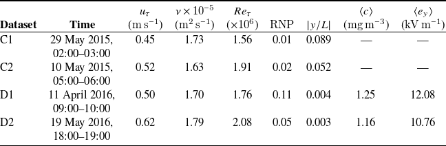
 uτ
 ν
 Reτ=uτδ/ν
 |y/L|
 ⟨c⟩
 ⟨ey⟩

 δ
 Lx
 Ly
 Lz
 Nx
 Ny
 Nz
 Δx
 Δy
 Δz
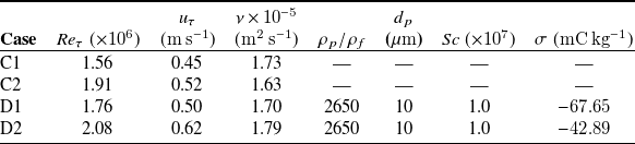
 Reτ
 uτ
 ν
 ρp/ρf
 dp
 Sc
 σ

 Q
 Q=20(Ub/δ)2

 ⟨u+⟩=(1/0.41)lny+−8.3
 u′rms+
 ⟨u′+v′+⟩

 y+=33750
 t+=tuτ2/ν=4.46×107
 u′+=u′/uτ
 c/⟨c⟩
 ey′/eν
 ⟨c⟩
 y+=33750
 eν=⟨ρe⟩δν/ε0
 δν=ν/uτ
 y+=956250
 1×10⁵δν

 ⟨u+⟩=(1/0.41)lny+−8.4
 ⟨u+⟩=(1/0.41)lny+−9.5
 u′rms+
 ⟨u′+v′+⟩
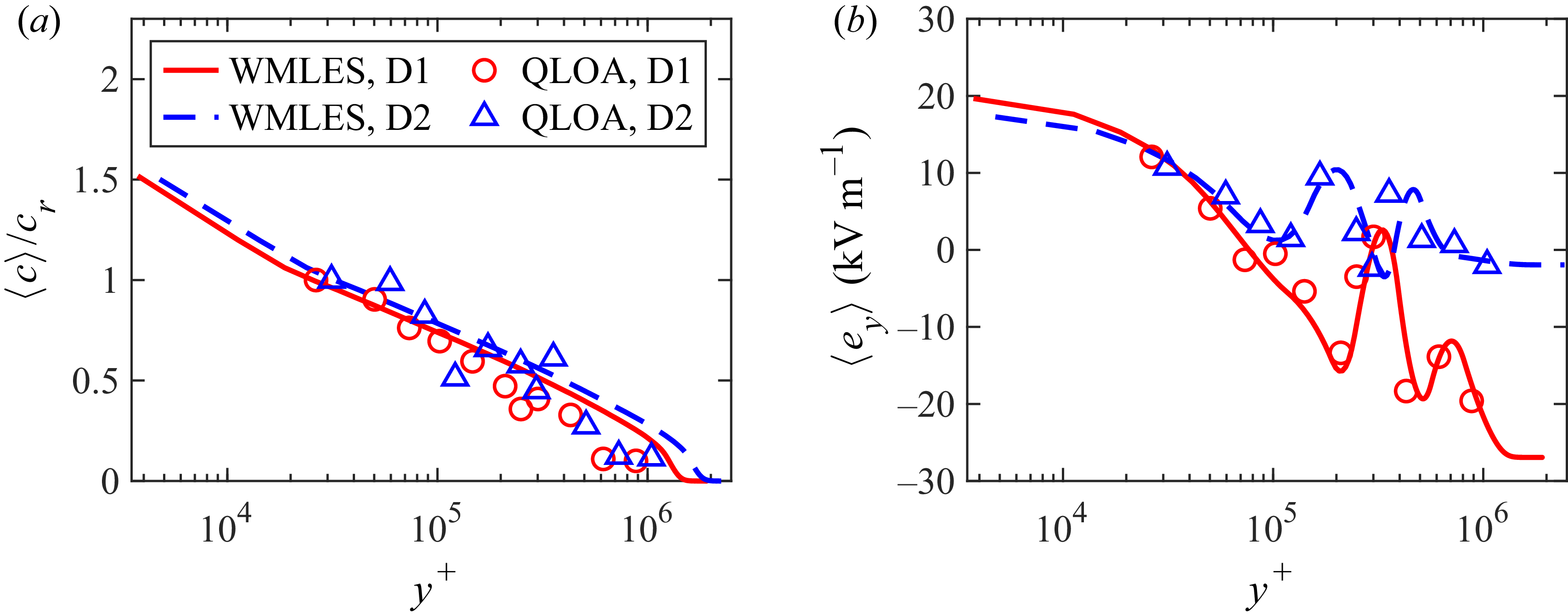
 ⟨c⟩/cr
 cr
 0.9 m
 ⟨ey⟩

 Scsgs
 Mclay
 ⟨c⟩/cr
 cr
 0.9 m
 ⟨c⟩
 ⟨ey⟩
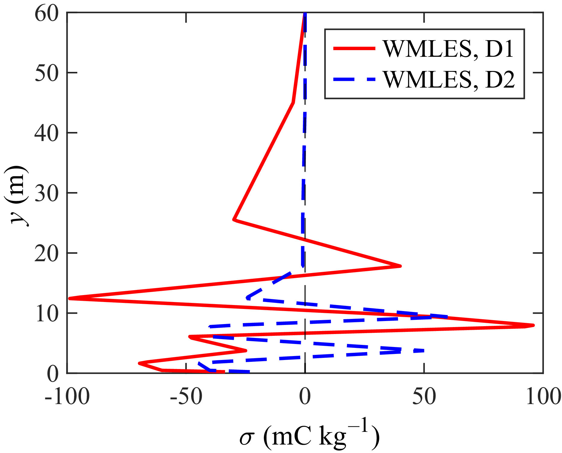
 σ(y)

 ⟨u+⟩
 u′rms+
 ⟨u′+v′+⟩
 ⟨c⟩/cr
 ⟨ey⟩
 Lx×Ly×Lz=4πδ×δ×2πδ

 Reτ=550
 u′rms+
 ⟨u′+v′+⟩
 ⟨c⟩
 ⟨ey⟩

 Open access

