2. The isothermal Euler equations

Consider a pipe of length $L>0$ that corresponds to the interval $[0,\, L]$ . Let $D>0$ denote the constant diameter of the pipe, $\lambda_{fric}\geq 0$ the friction coefficient and $\varphi\in {[\!-\!\pi,\,\pi]}$ the constant slope. Define $s_{lope}\;:\!=\;\sin\!(\varphi)$ and set $\theta\;:\!=\; \frac{\lambda_{\mathrm{fric}}}{D}$ . Let g denote the gravitational constant, $\rho>0$ the gas density, $p>0$ the pressure and q the cross-sectional mass flow rate.

We assume that we have a real gas that satisfies the state equation:

\begin{equation*}p = Z(p)\, R^e_s \, T^e\,\rho,\end{equation*}

where Z(p) is the compressibility factor that is given by a continuously differentiable function with strictly positive values, $R^e_s$ is the gas constant and $T^e$ is the temperature. The starting point of our study are the isothermal Euler equations (see for example [Reference Hante, Leugering, Martin, Schewe and Schmidt13]):

(2.1) \begin{equation}\left\{\begin{array}{l}\rho_t + q_x = 0,\\[5pt] q_t + \left( p + \dfrac{q^2}{\rho} \right)_x = - \dfrac{1}{2} \theta \dfrac{q \; |q|}{\rho}- \rho\, g \, s_{lope},\end{array}\right.\end{equation}

that govern the flow through a single pipe.

In our analysis, we also make use of the velocity $v= \dfrac{q}{\rho}$ and the sound speed c given by:

\begin{equation*} \left( \frac{1}{c} \right)^2 = \frac{\partial \rho}{\partial p} =\frac{1} {R^e_s \, T^e} \frac{\partial}{\partial p}\!\left( \frac{ p }{ Z(p)} \right) = \frac{1}{ R^e_s\, T^e} \frac{ Z(p) - p \, Z'(p)}{(Z(p))^2}.\end{equation*}

Thus, we have

\begin{equation*}c = \sqrt{R^e_s\, T^e} \, Z(p) \,\frac{1}{\sqrt{ Z(p) - p \, Z'(p) }}.\end{equation*}

For the Mach number M, this yields

\begin{equation*}M = \frac{v}{c}=q \, \sqrt{R^e_s\, T^e} \, \frac{\sqrt{ Z(p) - p \, Z'(p) }}{p}.\end{equation*}

The gas pipelines are operated in a subsonic flow regime where the absolute value of the velocity of the gas is strictly less than the sound speed in the gas. For the Mach number, we thus have

\begin{equation*}|M|\!<1.\end{equation*}

In fact, in the operation of gas transportation networks, upper bounds for the velocity of the gas are enforced. In order to state (2.1) in terms of the dimensionless Mach number M and the pressure p, we observe that

\begin{eqnarray*}\rho = \frac{1}{c^2} \,p \, \frac{1}{1 - p \,\left({\rm ln}(Z(p))\right)'}& &q = \frac{1}{c} \, M \,p\,\frac{1}{ 1 - p \left( {\rm ln}(Z) \right)'}.\end{eqnarray*}

If $M\not=0$ , then the first equation of (2.1) yields

\begin{equation*}\left[ Z(p) - p \, Z'(p) \right] p_t + (R^e_s\, T^e) Z(p)^2 \, q_x =0.\end{equation*}

This implies in turn

(2.2) \begin{equation} p_t + c^2 \, q_x =0. \end{equation}

We also have

\begin{equation*}\frac{q^2}{\rho} = M^2\,p \,\frac{1}{1 - p \,({\rm ln}(Z(p)))'}.\end{equation*}

Therefore,

\begin{equation*}\left(\frac{q^2}{\rho}\right)_x=M \left[ (2 \, p \, M_x + M \, p_x) \frac{Z(p)}{Z(p) - p \, Z'(p)}+ M\, p \, \left(\frac{Z(p)}{Z(p) - p \, Z'(p)}\right)_x\right].\end{equation*}

Hence, there is a continuous function $\aleph \;:\; {\mathbb R}^4 \rightarrow {\mathbb R}$ such that $\left(\frac{q^2}{\rho}\right)_x =M \, \aleph(M,\, P,\, M_x,\, p_x)$ and $\aleph(0)=0$ . This is the motivation to truncate for subsonic flow with small values of $|M|$ the term $\left(\frac{q^2}{\rho}\right)_x$ from the quasilinear model and to replace the second equation in (2.1) by:

(2.3) \begin{equation} q_t + p_x = - \frac{1}{2} \theta \, c^2 \,\frac{q \; |q|}{p}- g \, s_{lope} \, \frac{p}{ c^2}. \end{equation}

A derivation of this model using asymptotic expansions can be found in [Reference Brouwer, Gasser and Herty2].

3. The model for slow subsonic flow and the stationary states

With (2.2) and (2.3), the well-known model can be obtained (see for example [Reference Gugat, Leugering, Martin, Schmidt, Sirvent and Wintergerst7, Reference Herty, Mohring and Sachers14]):

(3.1) \begin{equation}\left\{\begin{array}{l}p_t + c^2 \, q_x = 0,\\[5pt] q_t + p_x = - \frac{1}{2} \theta \, c^2 \,\frac{q \; |q|}{p}- g \, s_{lope} \, \frac{p}{ c^2}.\end{array}\right.\end{equation}

For the case of ideal gas where $Z=1$ , this is a semilinear model. In [Reference Gugat and Ulbrich8], for the initial data $q(0,\, x)=0$ , $\rho(0,\, x) = \exp\!(\beta\, x)$ the solution of both the quasilinear model (2.1) and the semilinear model are given, which allows us to observe how the difference between the two solutions can grow exponentially fast with time.

Since the first equation in (2.1) has not been modified, also (3.1) guarantees the conservation of mass.

The stationary solutions of the quasilinear system (2.1) have been studied in [Reference Gugat, Hante, Hirsch-Dick and Leugering6] and [Reference Gugat, Wintergerst and Schultz10]. For the stationary states of system (3.1), we have $q = const.$ and $ p_x = - \frac{1}{2} \, \theta \,c^2\, \frac{q\, |q|}{p}- g \, s_{lope}\,\frac{1}{c^2} p.$ For a horizontal pipe (that is $ s_{lope}=0$ ), we get

\begin{equation*}\frac{1}{c^2} \,p \, p_x = - \frac{1}{2}\, {\rm sign}(q) \, \theta\,q^2.\end{equation*}

Thus, for the case of ideal gas where c is constant for $x\in [0,\,L]$ , we obtain

\begin{equation*}\frac{p^2}{2}(x) - \frac{p^2}{2}(0) = - \frac{1}{2}\, {\rm sign}(q) \, \theta \,c^2\, q^2\, x.\end{equation*}

This is the well-known Weymouth equation. We have $0 \leq \frac{p^2}{2}(x) =\frac{p^2}{2}(0) - \frac{1}{2}\, {\rm sign}(q) \, \theta \,c^2\, q^2\, x.$ Hence, for $q>0$ , the equation is a valid model only if x and consequently $L>0$ are sufficiently small. In fact, we can compute the point $x^\ast$ where the solution blows up. It satisfies the equation $0 = \frac{p^2}{2}(0) - \frac{1}{2}\, {\rm sign}(q) \, \theta \,c^2\, q^2\, x^{\ast}.$ Thus, we have $p(x^\ast)=0$ , so before this point is reached, the state ceases to be subsonic. Note that at the point $x^\ast$ , the derivative of p(x) blows up.

Also, in the original model (2.1), for the stationary states a blow-up of the derivative occurs after a finite length; see [Reference Gugat, Hante, Hirsch-Dick and Leugering6].

Now we consider the case where $s_{lope}\not=0$ . First, we consider constant stationary states. The constant stationary solutions corresponds to a constant flow rate $\bar q$ and a constant pressure $\bar p>0$ with

\begin{equation*} \bar p^2 = \frac{ c^4 \, \theta \bar q^2}{ 2 \, g \, |s_{lope}| }. \end{equation*}

For ideal gas, there exist stationary solutions with a constant flow rate $\bar q$ that satisfies

(3.2) \begin{equation} {\rm sign}(\bar q) = - {\rm sign}(s_{lope}), \end{equation}

where the pressure is given by:

\begin{equation*}p(x) = \bar p \; \sqrt{ 1 + \hat C \, \exp\!\left( - 2 \, g \,\frac{ s_{lope} }{c^2}\, x\right)},\end{equation*}

as long as the term under the square root is positive with $\hat C$ chosen such that $p(0)>0$ has the appropriate value. This can be verified by inserting the solution $(\bar q, p(x))$ into (3.1). This is a particular steady state where in the source term the friction part and the slope part cancel each other. More precisely, the definition of p implies

\begin{equation*} \frac{(p(x))^2 - \bar p^2}{\bar p^2} = \hat C \, \exp\! \left( - 2 \, g \,\frac{ s_{lope} }{c^2}\, x\right). \end{equation*}

Hence, due to the definition of $\bar p$ , we have

\begin{eqnarray*}p'(x)& = & \frac{ \bar p^2 }{2} \,\frac{1}{p(x)} \; \hat C \, \exp\! \left( - 2 \, g \,\frac{ s_{lope} }{c^2}\, x\right)\, \left( - 2 \, g \,\frac{ s_{lope} }{c^2} \right)\\[5pt] &=&\frac{ \bar p^2 }{2} \,\frac{1}{p(x)} \, \left(\frac{(p(x))^2}{\bar p^2} - 1 \right)\, \left( - 2 \, g \,\frac{ s_{lope} }{c^2} \right)\\[5pt] & = & 2 \, g \,\frac{ s_{lope} }{c^2}\frac{ \bar p^2 }{2} \, \,\frac{1}{p(x)} - \frac{ 1 }{2} \, 2 \, g \,\frac{ s_{lope} }{c^2}\, p(x)\\[5pt] & = &{\rm sign}(s_{lope})\, \frac{1}{2} \theta \, c^2 \,\frac{\bar q^2}{p(x)}- g \, s_{lope} \, \frac{p(x)}{ c^2}.\end{eqnarray*}

Whence, the relation (3.2) implies that the second equation in (3.1) holds.

4. The semilinear model in diagonal form

In the following, we restrict our considerations to the case of an ideal gas, where c is a constant and (3.1) is a semilinear model. Under this condition, the hyperbolic system can be elegantly rewritten to see that the characteristic curves are straight lines. This allows us to analyse the problem substantially.

We therefore state (3.1) in terms of the corresponding Riemann invariants, which are defined as:

\begin{equation*}R_\pm \;:\!=\; \pm p + M\, p = (\!\pm 1 + M)\, p.\end{equation*}

Hence, the physical variables can be expressed in terms of the Riemann invariants as:

\begin{equation*}p = \frac{R_+ - R_-}{2},\;M = \frac{R_+ + R_-}{R_+ - R_-},\end{equation*}

and we have the flow rate:

\begin{equation*}q = \frac{1}{c} M \, p= \frac{1}{2\, c} (R_+ + R_-).\end{equation*}

Let us further define some notation. Let $\sigma(z) \;:\!=\; z \, |z|$ and consider the function:

(4.1) \begin{equation} F(x, \, y)\;:\!=\;(x + y) \,\left| \frac{ x + y}{ x - y} \right|=(x - y) \,\sigma\left( \frac{ x + y}{ x - y} \right).\end{equation}

Then, in terms of the Riemann invariants, the system has the diagonal form:

(4.2) \begin{equation}(R_\pm)_t \pm c (R_\pm)_x =-\frac{1}{4} \theta \, c \; F(R_+,R_-)- g \, s_{lope}\,\frac{1}{c}\,\frac{R_+ - R_-}{2},\end{equation}

which is well defined as long as $R_+ \not = R_-$ . In terms of the physical variables, this is equivalent to $p>0$ . This requirement is often satisfied in applications as a lower bound $\underline p>0$ for the pressure is usually prescribed. In the subsonic flow regime, pressure constraints of the form:

(4.3) \begin{equation} \underline{p}\leq p \leq \bar{p}\end{equation}

can be expressed in terms of the Riemann invariant as:

(4.4) \begin{equation} 2\underline{p}\leq R_+ - R_- \leq 2\bar{p}.\end{equation}

Similarly, whenever $2p = R_+ - R_- > 0$ , the Mach number constraint

(4.5) \begin{equation} |M|\leq\lambda,\quad 0<\lambda<1,\end{equation}

is equivalent to

(4.6) \begin{align} (1+\lambda)R_+ + (1-\lambda)R_- &\geq 0,\end{align}

(4.7) \begin{align} (1-\lambda)R_+ + (1+\lambda)R_- &\leq0. \end{align}

Moreover, with $p>0$ , it is easy to see that $|M|<1$ implies that $R_+>0$ and $R_-<0$ . Note that all the constraints for the Riemann invariants are linear. This is convenient for associated optimal control problems for gas networks. The diagonal form (4.2) of the system has a similar structure as in [Reference Gugat and Ulbrich9]. The fundamental difference is that the Riemann invariants in (4.2) depend linearly on $(p,\, q)$ , whereas in [Reference Gugat and Ulbrich9] the Riemann invariants depend on the logarithm of the pressure. This stems from the study of the the diagonal form of the quasilinear system (2.1), where the diagonal matrix depend on the system state.

5. Existence of solutions of the semilinear model

In this section, we prove the existence of solutions of the initial boundary value problem with the semilinear model. The characteristic curves for the semilinear model are a priori given straight lines. For a given pair (x, t), $t \geq 0$ , we define the ${\mathbb R}^2$ -valued function $\xi_\pm(s,\, x,\, t)$ as the solution of the initial value problem:

\begin{equation*}\left\{\begin{array}{r}\xi_\pm(t,\, x,\, t)= (t,\, x),\\[5pt] \partial_s \xi_\pm(t,\, x,\, t) = ( 1,\, \pm c).\end{array}\right.\end{equation*}

Then, the characteristic lines passing through (x, t) are given by:

\begin{equation*}\xi_+(s,\, x,\, t)= (s,\, x + c (s-t))\quad \text{and}\quad \xi_-(s,\, x,\, t)= (s,\, x - c (s-t)).\end{equation*}

Along these lines, the hyperbolic system is equivalent to the following system for any s:

(5.1) \begin{equation} R_{\pm}\circ \xi_\pm(s,\, x,\, t) = R_{\pm}(t, x) - \int_t^s\left[ \frac{\theta \, c}{4} \, F(R_+,\, R_-)+ \frac{ g \, s_{lope} }{2c}(R_+ - R_-)\right]\!(\xi_\pm(\tau,\, t,\, x)) \,\mathrm{d} \tau.\end{equation}

This allows to prove the existence of continuous solutions for continuous problem data using a fixed-point iteration on (5.1). The existence of broad solutions of the semilinear system has already been shown in [Reference Hintermüller and Strogies15] for the case of horizontal pipes. In [Reference Hintermüller and Strogies15], Proposition 4, lower and upper bounds for the pressures and for the flow rate are considered. Indirectly, this also yields bounds for the gas velocity and the Mach number. In this paper, in contrast to [Reference Hintermüller and Strogies15], we include sloped pipes in our analysis. Since the semilinear model is only valid for sufficiently small Mach numbers, we also include constraints for the Mach number directly in the analysis. We point out that such a constraint for the velocity of the gas is also used in practice to avoid vibrations of the pipelines; see [Reference Freitas Rachid and Costa Mattos4] and [Reference Zou, Cheraghi and Taheri23] for studies of fluid-induced vibrations of natural gas pipelines. Note that in our result, all the constants in the assumptions are given explicitly, so they can be verified rather easily. Our result provides conditions that allow to obtain continuous solutions that satisfy the box constraints for the pressure and the Mach number. The conditions require continuous initial and boundary data that satisfy certain inequalities. Note that it is not sufficient to require that the initial and boundary data satisfy the state constraints for the pressure and the Mach number. This can be seen as follows: for a stationary state in a horizontal pipe, the pressure is decreasing along the pipe in the direction of flow. Hence, the pressure at the inflow end must be strictly above the lower bound for the pressure in order to guarantee that the state constraint is satisfied throughout the pipe.

In the forthcoming analysis, we invoke the inequality:

(5.2) \begin{equation} \frac{\theta\lambda\sqrt{5}}{2} + \frac{g |s_{\mathrm{lope}}|}{c^2} \leq \frac{1}{L}\end{equation}

between the physical characteristics of the pipe. The explicit character of this condition departs from the ones previously used for investigating the existence of solution, albeit with higher regularity.

Now we state our existence result.

Theorem 5.1. Consider a pipe with physical parameters $L > 0$ , $\theta\geq 0$ and $s_{lope}$ . Let $T>0$ and the numbers $\underline p, \overline p$ such that $0<\underline p < \overline p$ be given. Define the sets:

\begin{align*}\Gamma_+ &= \{0\}\times [0,\, L] \cup [0,\, T] \times \{0\}\\[5pt] \Gamma_- &= \{0\}\times [0,\, L] \cup [0,\, T] \times \{L\},\end{align*}

and the points:

\begin{equation*}P_0^\pm(t,\, x) = \Gamma_\pm\cap\{\xi_\pm(s,\, x,\, t), \, s\in \mathbb{R}\}\in {\mathbb R}^2.\end{equation*}

For the t-component of $P_0^\pm(t,\, x)$ , we use the notation $t_0^\pm(t,\, x)\geq 0$ .

Let a continuous state $R_+$ on $\Gamma_+$ , a continuous state $R_-$ on $\Gamma_-$ and a number $\lambda \in (0,\, 1)$ be given. Assume that there exists a number $\Delta t>0$ such that the values of $R_+$ and $R_-$ satisfy the inequalities:

(5.3) \begin{equation}R_+(P_0^+(t,\, x)) -R_-(P_0^-(t,\, x))\leq2\, \overline p\left( 1 -\frac{\theta \,c\,\Delta t}{2} \,\lambda^2\right),\end{equation}

(5.4) \begin{equation}R_+(P_0^+(t,\, x)) -R_-(P_0^-(t,\, x))\geq 2\, \underline p\left( 1 +\frac{\theta \,c\,\Delta t}{2} \,\lambda^2\frac{\overline p }{\underline p}\right).\end{equation}

Define the constant:

\begin{equation*}\hat U=\frac{1}{2} \theta \, c \,\lambda^2+ \frac{ g \, s_{lope} }{c}.\end{equation*}

Assume that $s_{lope}\leq 0$ and

(5.5) \begin{equation}\hat U\geq 0,\end{equation}

(5.6) \begin{equation}\frac{(1-\lambda) \,R_+(P_0^+(t,\, x))+(1 + \lambda) \,R_-(P_0^-(t,\, x))}{2\, \Delta t\,\overline p }\leq-\frac{1}{2} \theta \, c \,\lambda^2- \frac{ g \, |s_{lope}| }{c}\end{equation}

and

(5.7) \begin{equation}(1+\lambda) \,R_+(P_0^+(t,\, x))+(1 - \lambda) \,R_-(P_0^-(t,\, x))\geq 2\,\Delta t\,\overline p \,\hat U\end{equation}

for all $(t,\,x) \in [0,\, T]\times [0, \, L]$ . Moreover, assume that $\Delta t$ is sufficiently small in the sense that

(5.8) \begin{equation}\Delta t\,\left[\frac{\sqrt{5}}{2}\,\theta \, c\,\lambda + \frac{g \, |s_{lope}|}{ c} \right]< 1.\end{equation}

Then, with the given values of $R_+$ on $\Gamma_+$ and $R_-$ on $\Gamma_-$ that prescribe initial conditions at $t=0$ and boundary conditions at $x=0$ and $x=L$ , there exists a unique solution on $[0,\, \min\{T,\,\Delta t\}]$ given by continuous functions $R_+(t,\, x)$ , $R_-(t,\, x)$ for $t\in [0,\, \min\{T,\,\Delta t\}]$ and $x\in [0,\, L]$ that satisfy the hyperbolic system (4.2) in the sense of (5.1). The solution is subsonic, and the absolute value of the Mach number is less than or equal to $\lambda$ . The values of the pressure are contained in the interval $[\underline p,\; \overline p]$ .

Furthermore, if $\Delta t\geq \frac{L}{c}$ , thus in particular if (5.2) holds, the solution exists on $[0,\, T]$ .

Proof. Let a continuous function $R =(R_+,\, R_-)$ with $R_+$ , $R_- \in C([0,\, T]\times [0, \, L],\; \mathbb R)$ be given that satisfies the conditions (5.3), (5.4), (5.6), (5.7), as well as the box constraints (4.4)–(4.7). Define the operator $P\;:\!=\;(P_+,\, P_-)$ with

\begin{equation*}P_\pm(R)(t,\, x)=R_\pm(P_0^\pm(t,\, x))-\int_{t_0^\pm(t,x)}^t\left[\frac{1}{4} \theta \, c \, F(R_+,\, R_-)+ \frac{ g \, s_{lope} }{c}\frac{R_+ - R_-}{2}\right]\!(\xi_\pm(s,\, t,\, x)) \,\mathrm{d} s.\end{equation*}

Our first step is to check that P(R) satisfies, in terms of physical variables, the box constraints for the pressure and the bound for the Mach number, that is

(5.9) \begin{equation}2\, \underline p \leq(P_+ - P_-)(R)\leq 2\, \overline p,\end{equation}

and

(5.10) \begin{equation}\left|\frac{(P_+ + P_-)(R)}{(P_+ - P_-)(R)}\right| \leq \lambda,\end{equation}

are satisfied. Note that since $\lambda<1$ and $(P_+ - P_-)(R) > 0$ , the relation (5.10) implies $P_+(R) > 0$ and $P_-(R) < 0$ . Due to (5.5) we have

\begin{equation*}P_\pm(R)(t,\, x)\geq R_\pm(P_0^\pm(t,\, x))-\left(t - t_0^\pm(t,\, x)\right)\!\left(\frac{1}{2} \theta \, c \,\lambda^2+ \frac{ g \, s_{lope} }{c}\right)\overline p.\end{equation*}

Moreover, we have

\begin{align*}P_\pm(R)(t,\, x)\leq R_\pm(P_0^\pm(t,\, x))+\left(t - t_0^\pm(t,\, x)\right)\!\left(\frac{1}{2} \theta \, c \,\lambda^2+ \frac{ g \, |s_{lope}| }{c}\right)\overline p.\end{align*}

Hence, if $t - t_0^\pm(t,\, x) \leq \Delta t$ and $s_{lope}\leq 0$ , inequality (5.3) implies

\begin{equation*}(P_+ - P_-)(R) \leq R_+(P_0^+(t,\, x)) -R_-(P_0^-(t,\, x))+ \overline p \,\theta \,c \,\Delta t \,\lambda^2\,\leq 2\, \overline p.\end{equation*}

Similarly, we have the inequality:

\begin{equation*}(P_+ - P_-)(R) \geq R_+(P_0^+(t,\, x)) - R_-(P_0^-(t,\, x))-\left(t - t_0(t,\, x)\right)\, \theta \, c \,\lambda^2\, \overline p.\end{equation*}

Hence, (5.4) implies

\begin{equation*}(P_+ - P_-)(R) \geq 2\, \underline p.\end{equation*}

and P(R) satisfies (5.9). Furthermore, we have $(P_+ - P_-)(R)\geq 2 \, \underline{p} > 0$ . This implies that the Mach number constraint (5.10) can expressed as in (4.6)–(4.7), that is:

(5.11) \begin{align} (1 - \lambda ) \, P_+(R) + (1 + \lambda) \,P_-(R) \leq & 0, \end{align}

(5.12) \begin{align} (1 + \lambda ) \, P_+(R) + (1 - \lambda) \, P_-(R)\geq & 0. \end{align}

For the first inequality, we obtain

\begin{align*} (1 - \lambda ) \, P_+(R) + (1 + \lambda) \, P_-(R) & \leq (1 - \lambda )\, R_+(P_0^+(t,\, x)) + (1 + \lambda) \, R_-(P_0^-(t,\, x)) \\[5pt] &\qquad +2 \,\Delta t\,\left(\frac{1}{2} \theta \, c \,\lambda^2+ \frac{ g \, |s_{lope}| }{c}\right)\overline p.\end{align*}

Due to (5.6), this implies

\begin{equation*}(1 - \lambda ) \, P_+(R) + (1 + \lambda) \, P_-(R) \leq 0.\end{equation*}

For the second inequality, we have

\begin{align*}(1 + \lambda ) \, P_+(R) + (1 - \lambda) \, P_-(R)& \geq(1 + \lambda )\, R_+(P_0^+(t,\, x)) +(1 - \lambda) \, R_-(P_0^-(t,\, x))\\[5pt] &\qquad - 2 \,\Delta t\,\left(\frac{1}{2} \theta \, c \,\lambda^2 \,+ \frac{ g \, s_{lope} }{c}\right)\overline p.\end{align*}

Due to (5.7), this implies

\begin{equation*}(1 + \lambda ) \, P_+(R) + ( 1 - \lambda) \, P_-(R) \geq 0.\end{equation*}

Remember that with $(P_+ - P_-)(R) > 0$ , the inequality (5.10) implies that $P_+(R) > 0$ , and $P_-(R) < 0$ . By Lemma A.2, P(R) is continuous.

So we can start a fixed-point iteration with the operator P where each iterate satisfies (5.9)–(5.10). It remains to show that the fixed-point iteration is convergent. However, this is standard. In fact for a continuous function that satisfies (5.9), (5.11)–(5.12), and $S_+ = R_+$ on $\Gamma_+$ and $S_- = R_-$ on $\Gamma_-$ , we have

\begin{align*}|P_+(R) - P_+(S)|(t,\, x) & \leq \frac{\theta \, c}{4}\int_{t_0^\pm(t,\, x))}^t\left|F(R_+,\, R_-) - F(S_+,\, S_-)\right|(\xi_+(s,\, t,\, x)) \,\mathrm{d} s\\[5pt] &\quad +\int_{t_0^\pm(t,\, x))}^t\left|\frac{g \, s_{lope}}{c}\frac{(R_+ - S_+) - (R_- - S_-) }{2}\right|(\xi_+(s,\, t,\, x)) \,\mathrm{d} s.\end{align*}

Note that we can invoke Lemma A.1 to get the estimate

\begin{gather*}|P_+(R) - P_+(S)|(t,x)\leq \left[\frac{\sqrt{5}}{2}\theta c\lambda + \frac{g s_{\mathrm{lope}}}{c}\right]|t - t^0_+(t,x)| \max \{|R_+ - S_+|, |R_- - S_-|\}.\end{gather*}

For $P_-$ a similar estimate holds. Hence, if $|t - t_0(t,\, x)|\leq \Delta t$ , due to (5.8) we have

\begin{equation*} \Delta t\,\left[\frac{\sqrt{5}}{2}\,\theta \, c\,\lambda + \frac{g \, |s_{lope}|}{c} \right]< 1,\end{equation*}

which implies that P is a contraction. Hence, Banach’s fixed-point theorem yields the existence of a continuous solution on the corresponding short time interval contained in $[0,\,\Delta t]$ .

Note that due to the construction, we have the upper bound $|t - t_0(t,\, x)|\leq \frac{L}{c}$ . Hence, if the assumptions hold with $\Delta t\geq \frac{L}{c}$ , we obtain a contraction on $[0,\, T]\times [0,\, L]$ which implies that the solution exists on the interval $[0,\, T]$ where T can be chosen arbitrarily large.

Thus, we have proven Theorem 5.1.

6. Constrained exact controllability

In the operation of gas networks when the customer demand changes from an initially constant demand to a new constant demand, it is necessary to steer the system from a stationary initial state to a desired terminal state in such a way that the imposed state constraints for the pressure and velocity remain valid. While there are numerous results about exact controllability (see for example [Reference Li and Zhang18]), to our knowledge the exact boundary controllability with state constraints has not yet been analysed for hyperbolic systems. Exact boundary controllability with control constraints has been studied for example in [Reference Klamka16].

We want to analyse the problem of state-constrained exact boundary controllability between stationary states in the framework of continuous solutions on $\Omega = [0,T]\times[0,L]$ . To this end, we divide this domain into four pieces, as shown on Figure 1. Note that an initial stationary state $R^{(0)}_\pm$ completely determines the system state on the triangle:

\begin{equation*}D_{\mathrm{I}}\;:\!=\; \{(t,\, x)\;:\; t\geq 0,\; x\in [0,\, L], \; c \, t \leq x,\;c \, t\leq L-x \}.\end{equation*}

If the state constraints hold for the initial state, they are also satisfied on $D_{\mathrm{I}}$ . Similarly, for $T > L/c$ , a desired stationary terminal state $R^{(T)}_\pm$ completely determines the system state on the triangle:

\begin{equation*}D_{\mathrm{II}}\;:\!=\; \{(t,\, x)\;:\; t \in [0,\, T],\; x\in [0,\, L], \;c \, (T- t) \leq x,\;c \, (T- t) \leq L-x \}.\end{equation*}

Again if the state constraints hold for the terminal state, they are also satisfied on $D_{\mathrm{II}}$ .

Figure 1.

Domain and boundaries for the exact controllability boundary analysis.

In order to construct exact boundary controls that steer the system from $R^{(0)}_\pm$ to $R^{(T)}_\pm$ , we define a new state $R^{\mathrm{mid}}_\pm$ on the $I_{\mathrm{mid}}$ segment which joins the inner vertices of the $D_{\mathrm{I}}$ and $D_{\mathrm{II}}$ triangles. More precisely, this segment is defined as:

\begin{equation*} I_{\mathrm{mid}} \;:\!=\; \left[\frac{L}{2c}, T-\frac{L}{2c}\right]\times\left\{\frac{L}{2}\right\}.\end{equation*}

One possibility for the values of $R^{\mathrm{mid}}_\pm$ is to use a convex combination of the values at the aforementioned vertices. For the forthcoming analysis, we use the following boundaries:

\begin{alignat*}{2} \Gamma^{\mathrm{III}}_+ &\;:\!=\; I_{\mathrm{mid}} \cup \left\{\left(T-\frac{y}{c}, y\right) \mid 0\leq y\leq \frac{L}{2}\right\},\quad && \Gamma^{\mathrm{III}}_- \;:\!=\; I_{\mathrm{mid}} \cup \left\{\left(\frac{y}{c}, y\right) \mid 0\leq y\leq \frac{L}{2}\right\},\\[5pt] \Gamma_+^{\mathrm{IV}} &\;:\!=\; I_{\mathrm{mid}} \cup \left\{\left(\frac{y}{c}, L-y\right) \mid 0\leq y\leq \frac{L}{2}\right\},\quad && \Gamma_-^{\mathrm{IV}} \;:\!=\; I_{\mathrm{mid}} \cup \left\{\left(T-\frac{y}{c}, L-y\right) \mid 0\leq y\leq \frac{L}{2}\right\}.\end{alignat*}

Now, we can exchange the roles of t and x and consider a leftward initial boundary value problem on the set:

\begin{equation*}R^{\mathrm{III}} \;:\!=\; [0, T]\times \!\left[0, \frac{L}{2}\right]\backslash (D_{\mathrm{I}} \cup D_{\mathrm{II}}),\end{equation*}

with ‘initial’ data from the stationary states $R^{(0)}_\pm$ , $R^{(T)}_\pm$ on $\Gamma^{\mathrm{III}}_\pm\cap D_{I}$ , $\Gamma^{\mathrm{III}}_\pm\cap D_{II}$ , respectively and $R^{\mathrm{mid}}_{\pm}$ on $I_{\mathrm{mid}}$ . The PDE for the Riemannian invariants reads

(6.1) \begin{equation}(R_\pm)_x \mp \frac{1}{c} \, (R_\pm)_t = - \frac{1}{4} \theta F(R_+,R_-)- g \, s_{lope}\,\frac{R_+ - R_-}{2c^2},\end{equation}

where F is defined in (4.1). The plus component of the boundary trace of these solutions at $x=0$ yields a continuous boundary control $u_+(t)$ for $t\in (0, \, T)$ . The existence of solutions for such a problem, with the solution satisfying the state constraints, is dealt with in Proposition 6.1, under appropriate smallness assumptions for $R^{(T)}-R^{(0)}$ and on $\theta$ and $|s_{lope}|$ . The latter is addressed in (5.2), and the former is made precise in the forthcoming hypothesis (6.4)–(6.7).

Similarly, by considering a rightward initial boundary value problem for the hyperbolic system

(6.2) \begin{equation}(R_\pm)_x \pm \frac{1}{c} \, (R_\pm)_t = - \frac{1}{4} \theta F(R_+,R_-)- g \, s_{lope}\,\frac{R_+ - R_-}{2c^2},\end{equation}

on the set

\begin{equation*}R^{\mathrm{IV}}\;:\!=\; [0, T]\times [x_0,\, L]\backslash (D_{\mathrm{I}} \cup D_{\mathrm{II}}),\end{equation*}

we obtain a continuous boundary control $u_-(t)$ for $t\in (0, \, T)$ as the minus component of the boundary trace of these solutions at $x=L$ .

Since we have reversed the roles of time and space, the integration is performed along the characteristics curves $\psi(y,t,x)$ , which satisfy the following ODE:

(6.3) \begin{equation} \left\{ \begin{aligned}\psi_\pm(x, t, x) &= (t, x),\\[5pt] \partial_y \psi_\pm(y, t, x) &= (\!\pm c^{-1}, 1).\end{aligned}\right.\end{equation}

These functions can be represented as:

\begin{align*} \psi_\pm(y, t, x) &= (t\pm c^{-1}(y - x), y).\end{align*}

The following proposition contains sufficient conditions that guarantee the existence of continuous solutions of the corresponding Goursat problems on $R^{\mathrm{III}}$ and $R^{\mathrm{IV}}$ , respectively.

Proposition 6.1. Consider a pipe with physical parameters $L > 0$ , $\theta \geq 0$ and $s_{lope}$ . Suppose that $T > L/c$ and (5.2) hold. Let $\tilde{U}\;:\!=\; \frac{1}{2}\theta\lambda^2 + \frac{g}{c^2} |s_{\mathrm{lope}}|$ . Furthermore, assume that the steady continuous initial state $R_{\pm}^{(0)}$ , the steady terminal state $R_{\pm}^{(T)}$ and the values on $I_{\mathrm{mid}}$ are such that the following inequalities hold

(6.4) \begin{align} R_+(\mathbf{P}^0_+(t,x)) - R_-(\mathbf{P}^0_-(t,x)) &\leq \bar{p}\left(2-\tilde{U}L\right), \end{align}

(6.5) \begin{align} R_+(\mathbf{P}^0_+(t,x)) - R_-(\mathbf{P}^0_-(t,x)) &\geq \underline{p} \left(2+\tilde{U} L\frac{\bar{p}}{\underline{p}}\right), \end{align}

(6.6) \begin{align} (1+\lambda)R_+(\mathbf{P}^0_+(t,x)) + (1-\lambda)R_-(\mathbf{P}^0_-(t,x)) &\geq L\,\bar{p}\,\tilde{U}, \end{align}

(6.7) \begin{align} (1-\lambda)R_+(\mathbf{P}^0_+(t,x)) + (1+\lambda)R_-(\mathbf{P}^0_-(t,x)) &\leq -L\,\bar{p}\,\tilde{U}, \end{align}

where the initial boundary domain $\mathbf{P}^0_\pm(t,x)$ is defined as:

\begin{equation*} \mathbf{P}^0_\pm(t,x) = \begin{cases} \left\{\Gamma^{\mathrm{III}}_{\pm} \cap \{\psi_\pm(y, t, x), y\in\mathbb{R}\}\right\}&\text{for the domain $R^{\mathrm{III}}$},\\[5pt] \left\{ \Gamma^{\mathrm{IV}}_{\pm} \cap \{\psi_\pm(y, t, x), y\in\mathbb{R}\}\right\}&\text{for the domain $R^{\mathrm{IV}}$.}\end{cases} \end{equation*}

Then, given initial values on $\Gamma^{\mathrm{III}}_\pm$ (resp. $\Gamma^{\mathrm{IV}}_\pm$ ) there exists unique continuous functions $R_+$ , $R_-$ on the $R^{\mathrm{III}}$ (resp. $R^{\mathrm{IV}}$ ) domain that satisfies the integral version of system (6.1) (resp. (6.2)) along the characteristics and the box constraints (4.3) and (4.5).

Proof. For $|M|\!\leq \lambda$ , we have

\begin{equation*} \left|\frac{1}{2}\theta M|M| + \frac{g}{c^2}s_{\mathrm{lope}}\right| \leq \tilde{U}.\end{equation*}

Let us proceed with the analysis of the domain $\mathrm{R}^{\mathrm{III}}$ , for which the initial conditions are $\Gamma^{\mathrm{III}}_\pm$ . The choice of $\psi$ in (6.3) is such that

\begin{gather*} \frac{\mathrm{d}}{\mathrm{d}y}R_\pm \circ \psi_{\pm}(y, t, x) = \left((R_\pm)_x \mp c^{-1} (R_\pm)_t\right)\circ \psi_{\pm}(y, t, x)\\[5pt] = \left(-\frac{1}{2}\theta F(R_+,R_-) - g s_{lope} \frac{1}{c^2}\left(\frac{R_+ - R_-}{2}\right ) \right)\circ\psi_{\pm}(y, t, x).\end{gather*}

As in the proof of Theorem 5.1, we tackle the existence of solutions by using a fixed-point approach on $P\;:\!=\;(P_+,P_-)$ , defined as follows:

\begin{equation*} P_{\pm}(R_{\pm}(t,x)) \;:\!=\; R_{\pm}(P^0_{\pm}(t,x)) + \int_{x^0_{\pm}}^{x} \frac{\mathrm{d}}{\mathrm{d}y}R_\pm \circ \psi_{\pm}(y, t, x) \,\mathrm{d} y,\end{equation*}

with $P^0_{\pm}(t,x) \;:\!=\; \Gamma^{\mathrm{III}}_{\pm} \cap \{\psi_\pm(y, x, t), y\in\mathbb{R}\}$ is the initial boundary for the domain $R^{\mathrm{III}}$ (see Figure 1) and $x^0_\pm$ is the ‘space’ component of $P^0_\pm(t,x)$ , where the argument (t, x) on $x^0_\pm$ is dropped since there is no ambiguity. Note that by construction of the domain $R^{\mathrm{III}}$ , we have

(6.8) \begin{equation} |x(t,x) - x^0_{\pm}(t,x)|\; \leq \frac{L}{2}.\end{equation}

Finally, it holds that $R_{\pm}(P^0_{\pm}(t,x)) = R_{\pm} \circ \psi(x^0_{\pm}, t, x)$ .

Let a continuous function $R =(R_+,\, R_-)$ be given that satisfies the box constraints (4.4)–(4.7), and for which the hypothesis (6.4)–(6.7) and (5.2) hold. Let us denote the right-hand side in (6.1) by $f\circ R$ . Then, rewriting this function in terms of the pressure p and Mach number M, we get

\begin{align*} f(p,M) & = -\frac{1}{2}\theta p M |M| - \!g s_{\mathrm{lope}} \frac{p}{c^2}, \end{align*}

which leads to the upper bound:

(6.9) \begin{align} |f| & \leq \frac{1}{2}\theta\lambda^2 \bar{p} + g |s_{\mathrm{lope}}| \frac{\bar{p}}{c^2} = \tilde{U}\bar{p}.\end{align}

We continue our analysis by checking whether P(R) satisfies the following constraints:

(6.10) \begin{equation}2\, \underline p \leq(P_+ - P_-)(R)\leq 2\, \overline p,\end{equation}

and

(6.11) \begin{equation}\left|\frac{(P_+ + P_-)(R)}{(P_+ - P_-)(R)}\right| \leq \lambda,\end{equation}

on $R^{\mathrm{III}}$ . Note that if $(P_+ - P_-)(R) > 0$ and $\lambda<1$ , then the relation (6.11) implies $P_+(R) > 0$ and $P_-(R) < 0$ . Starting with (6.10), we get

\begin{align*} P_+(R)(t, x) - P_-(R)(t, x) & = R_+(P^0_+(t, x)) - R_-(P^0_-(t,x)) + \mbox{$\displaystyle\int_{x^0_+}^{x} f\circ R\circ\psi_{+}(y, t, x)\,\mathrm{d} y$} \\[5pt] &\quad - \int_{x^0_-}^{x} f\circ R\circ\psi_{-}(y, t, x)\,\mathrm{d} y.\end{align*}

Using (6.8) and (6.9), the magnitude of the difference of the integral terms can be bounded by $\tilde{U}L\bar{p}$ . Then, invoking hypothesis (6.4) and (6.5), we get

\begin{equation*} 2\underline{p} \leq P_+(R)(t, x) - P_-(R)(t, x) \leq 2\bar{p}.\end{equation*}

Now, let us move to the inequalities (6.11):

\begin{gather*} (1+\lambda)P_+(R)(t, x) + (1-\lambda)P_-(R)(t, x) = (1+\lambda)R_+(P^0_+(t, x)) + (1-\lambda)R_-(P^0_-(t,x))\\[5pt] + (1+\lambda)\displaystyle\int_{x^0_+}^{x} f\circ R\circ\psi_{+}(y, t, x)\,\mathrm{d} y + (1-\lambda)\int_{x^0_-}^{x} f\circ R\circ\psi_{-}(y, t, x)\,\mathrm{d} y.\end{gather*}

Note that the sum of the integral terms is also bounded in magnitude by $\tilde{U}\,L\,\bar{p}$ , for any value of $\lambda\in[\!-\!1,1]$ . Using hypothesis (6.6), we get

\begin{align*} (1+\lambda)P_+(R)(t,x) + (1-\lambda) P_-(R)(t,x) &\geq 0.\end{align*}

And similarly, using hypothesis (6.7), we have

\begin{align*} (1-\lambda) P_+(R)(t,x) + (1+\lambda)P_-(R)(t,x) &\leq 0.\end{align*}

Hence, along the characteristics, the constraints (6.10) and (6.11) are fulfilled as long as R satisfies the box constraints and the hypothesis (6.4)–(6.7) hold. Note that, by construction, $P_+(R)$ (resp. $P_-(R)$ ) is absolutely continuous on $\psi_{+}$ (resp. $\psi_{-}$ ).

We shall now show that P is a contraction. Remember that (6.10) and (6.11), with $\lambda<1$ , implies that $P_+(R) > 0$ and $P_-(R) < 0$ . We now consider continuous functions $R_\pm$ and $S_\pm$ fulfilling (4.4) and (4.6)–(4.7), and such that $S_+ = R_+$ on $\Gamma^{\mathrm{III}}_+$ and $S_- = R_-$ on $\Gamma^{\mathrm{III}}_-$ . Following the usual approach for studying contraction properties, we have

\begin{align*} |P_+(R) - P_+(S)|(t,x) \leq & \frac{\theta}{4}\int_{x^0_{+}}^x |F(R_+,R_-) - F(S_+,S_-)|\circ\psi_+(y,t,x) \,\mathrm{d} y\\[5pt] &\quad + \frac{g s_{\mathrm{lope}}}{2c^2} \int_{x^0_{+}}^x |R_+ - S_+ - R_- + S_-|\circ\psi_+(y,t,x) \,\mathrm{d} y.\end{align*}

Invoking Lemma A.1 yields the following estimate:

\begin{gather*}|P_+(R) - P_+(S)|(t,x)\leq \left[\theta \lambda\frac{\sqrt{5}}{2} + \frac{g s_{\mathrm{lope}}}{2c^2}\right]|x - x^0_+(t,x)| \;\max \{|R_+ - S_+|, |R_- - S_-|\}.\end{gather*}

For $P_-$ , the same estimate holds. Since $|x - x^0_+(t,x)|\leq \frac{L}{2}$ on $\mathrm{R}^{\mathrm{III}}$ , using (5.2) we get

\begin{equation*} |P_{\pm}(R) - P_{\pm}(S)|(t,x) \leq \frac{1}{2} \, \max \{|R_+ - S_+|, |R_- - S_-|\}.\end{equation*}

Hence, Banach fixed-point theorem asserts the existence of a unique continuous solution, which satisfies the box constraints.

For the domain $R^{\mathrm{IV}}$ , the proof is along the same line. The hyperbolic system is (6.2), with initial conditions now on $\Gamma^{\mathrm{IV}}_\pm$ . The operator $P\;:\!=\;(P_+,P_-)$ on $R^{\mathrm{IV}}$ reads

\begin{equation*} P_{\pm}(R_{\pm}(t,x)) = R_{\pm}(P^0_{\pm}(t,x)) + \int_{x^0_{\pm}}^{x} f \circ \psi_{\pm}(y, t, x) \,\mathrm{d} y,\end{equation*}

with $P^0_{\pm}(t,x) \;:\!=\; \Gamma^{\mathrm{IV}}_{\pm} \cap \{\psi_\pm(y, x, t), y\in\mathbb{R}\}$ . Note that the bound (6.9) is also valid for the term under the integral. Furthermore, the initial values $R_{\pm}(P^0_{\pm}(t,x))$ satisfy (6.4)–(6.7). Following the same steps as for $R^{\mathrm{III}}$ , we get that $P_+$ and $P_-$ satisfy (6.10)–(6.11). Additionally, the contraction proof for P goes through whenever (5.2) holds. Hence, in $R^{\mathrm{IV}}$ , there is also existence and uniqueness of a continuous solution satisfying the box constraints.

The above construction implies that with the continuous boundary controls $u_+$ at $x=0$ and $u_-$ at $x=L$ , the initial boundary value problem with the initial state $R^{(0)}$ has a continuous solution R on $[0,\, T]\times [0, \, L]$ that satisfies the state constraint on $[0,\, T]\times [0, \, L]$ and the terminal constraint:

\begin{equation*}R(T, x) = R^{(T)}(x).\end{equation*}

Thus, we have shown the following theorem on local constrained exact controllability:

7. Numerical experiments

We present some numerical results for the exact controllability between two stationary states and investigate two cases: the first one is an increase in the mass flow and the second one is an inversion of the direction of the flow. As for the analysis, we use the relations satisfied by the solutions along the characteristic lines as a basis for the numerical scheme. We focus on the $D_{\mathrm{I}}$ and $D_{\mathrm{II}}$ , and the relations are similar for $R^{\mathrm{III}}$ and $R^{\mathrm{IV}}$ . Let $(t_i, x_i)$ and $(t_j, x_j)$ be two distinct coordinates in either $D_{\mathrm{I}}$ or $D_{\mathrm{II}}$ . Let $(t_k, x_k)$ be the intersection of the $\xi_+$ and $\xi_-$ characteristics starting from $(t_i, x_i)$ and $(t_j, x_j)$ , respectively. Then, there exists $\Delta_+$ and $\Delta_-$ such that $\xi_+(t_i+\Delta_+, x_i, t_i) = \xi_-(t_j+\Delta_-, x_j, t_j) = (t_k, x_k)$ . Let $R^i_{\pm}\;:\!=\; R_\pm(t_i, x_i)$ , $R^j_{\pm}\;:\!=\; R_\pm(t_j, x_j)$ and $R^k_{\pm}\;:\!=\; R_\pm(t_k, x_k)$ . Using the midpoint rule for approximating the integral on the right-hand side in (5.1) yields

(7.1) \begin{equation} R^k_+ - R^i_+ = -\frac{\Delta_+}{2}\left[\frac{\theta \, c}{4} \, (F( R^i_+, R^i_-) + F(R^k_+, R^k_-)) + g \, s_{lope}\,\frac{R^i_+ - R^i_- + R^k_+ - R^k_-}{2c} \right]\!\!.\end{equation}

Similarly, we have the following relation for $R^j_-$ and $R^k_-$ :

(7.2) \begin{equation} R^k_- - R^j_- = -\frac{\Delta_-}{2}\left[\frac{ \theta \, c}{4} \,(F( R^j_+, R^j_-) + F(R^k_+, R^k_-)) + g \, s_{lope}\,\frac{R^j_+ - R^j_- + R^k_+ - R^k_- }{2c} \right]\!\!.\end{equation}

Hence, the numerical scheme for computing the values of the Riemann invariants at $(t_k, x_k)$ consists in finding a solution to the nonlinear (implicit) system formed by the previous two equations. Newton’s method is then used to compute a solution to this system. For this, we first need to define a set of points $\{(t_k, x_k)\}$ at which those quantities are evaluated. Since the right-hand side involves both $R_+$ and $R_-$ , the set of points must allow for the evaluation of both quantities. This is achieved by considering a ‘triangular’ grid, constructed in the following way: for the $D_{\mathrm{I}}$ and $D_{\mathrm{II}}$ domains, $N_D$ equidistant nodes are placed on the line segment corresponding to the initial (resp. terminal) state. Then, $N_D$ equidistant line segments, parallel to the y-axis, slice the triangle $D_{\mathrm{I}}$ (resp. $D_{\mathrm{II}}$ ) into $N_D-1$ convex isosceles trapezoids. The nodes in the grid are defined as the intersection of the characteristic lines starting from the $N_D$ nodes located on the initial (resp. terminal) state and the aforementioned vertical line segments. This also implies that both Riemann invariants are defined at the nodes, as well as pressures and Mach numbers. The number of nodes on each line segment is decreasing by one when moving away from the initial (resp. terminal) state. The distance between two consecutive nodes on a given characteristic is $\Delta s = \frac{L}{2 c (N_D-1)}$ . Note that this quantity is an output for a given choice of grid and not an input parameter for the construction of the grid.

The $R_{\mathrm{III}}$ and $R_{\mathrm{IV}}$ domains are also sliced into convex isosceles trapezoids by $N_R$ horizontal line segments, between $I_{\mathrm{mid}}$ and the $u_+$ (resp. $u_-$ ) boundary. It is also the number of nodes on any horizontal line segment of length $T_L$ and hence gives the distance $\Delta t = \frac{L}{2 c (N_R-1)}$ between nodes on $I_{\mathrm{mid}}$ . To simplify the numerical implementation, we round up the length of $I_{\mathrm{mid}}$ so that it is a multiple of $\Delta t$ . Then, the number of nodes on $I_{\mathrm{mid}}$ is $N_{\mathrm{mid}}$ and the number of nodes on each boundary $u_{\pm}$ is $N_{\mathrm{mid}} + N_R$ . The distance between two consecutive nodes on a given characteristic is $\Delta y = \frac{L}{2(N_R-1)}$ .

Proof. By construction of the triangular grid on $D_{\mathrm{I}}$ or $D_{\mathrm{II}}$ , we have $\Delta_+ = \Delta_- = \Delta s$ with $\Delta s = \frac{L}{2 c (N_D-1)}$ . Then, the system (7.1)–(7.2) can be rewritten as $G(R^k) = H(R^i,R^j)$ , where

\begin{equation*} G(R)\;:\!=\; R + \Delta s\left(\frac{\theta\, c}{8} \begin{pmatrix}1\\[5pt] 1\end{pmatrix}F(R) + \frac{g\, s_{lope}}{4\, c} \begin{pmatrix}1&1\\[5pt] 1&1\end{pmatrix}R\right), \end{equation*}

and $H(R^i,R^j)$ is the constant right-hand side. Invoking Lemma A.1, we get that F is $C^1$ on X and $\|\nabla F(R^*)\|_2\leq \sqrt{10}\lambda$ for any $R^*\in X$ . This yields that G is $C^1$ on X. Moreover, we have

\begin{equation*} \nabla G(R^*) = I + \Delta s \left(\frac{\theta\, c}{8} \begin{pmatrix}1\\[5pt] 1\end{pmatrix}\nabla F(R^*)^T + \frac{g\, s_{lope}}{4\, c} \begin{pmatrix}1&1\\[5pt] 1&1\end{pmatrix}\right), \end{equation*}

that is the sum of the identity matrix plus a perturbation whose norm is controlled by $\Delta s$ . Hence, there exists $\Delta s^* > 0$ such that for all $0 < \Delta s\leq \Delta s^*$ , the matrix $\nabla G(R^*)$ is positive definite. This yields a minimum number of nodes $N_D^* > 0$ and the proof is complete.

One of the property enjoyed by our numerical solution is its reversibility along the characteristics. This is easy to see from the system (7.1)–(7.2): the right-hand side has the same expression for both $R^i$ and $R^j$ . Hence, changing the integration interval from $t_k$ to $t_k-\Delta_+$ yields the same relation as (7.1), with just both sides negated. This implies that the boundary values computed by the forward/backward propagation of $I_{\mathrm{mid}}$ can be interpreted as control inputs. Indeed, assuming that $N_R = N_D$ , then integrating forward in time the pipe using those boundary values would give the desired terminal state. This is not the case with the explicit or implicit Euler discretisation of the right-hand side. Another consequence is that values of R on $\Gamma^{\mathrm{III}}_\pm$ and $\Gamma^{\mathrm{IV}}_\pm$ must coincide, in particular outside of $I_{\mathrm{mid}}$ . By construction, this is true for either $R_+$ or $R_-$ , and this was numerically verified for the other component of R at a very high numerical accuracy.

The set-up for the numerical simulations is as follows: the pipe length $L=1000\;\mathrm{km}$ , $D = 1\;\mathrm{m}$ , $T = 15^{\circ}$ , $R_s = 518.26\;\mathrm{J\,kg}^{-1}\mathrm{K}$ , $\lambda_{\mathrm{fric}} = 2\times 10^{-6}$ . This gives $c = 386.44\;\mathrm{ms}^{-1}$ and $T_L = 2587.71\;\mathrm{s}$ . The large pipe length is there to further highlight the effect of the nonlinear source term.

Example 7.2. With this pipe, we first compute the controls for increasing the flow rate in the pipe from $q_0 = 100\;\mathrm{kg\,s}^{-1}\mathrm{m}^{-2}$ to $q_T = 1000\;\mathrm{kg\,s}^{-1}\mathrm{m}^{-2}$ , while keeping a pressure of $p = 50\;\mathrm{bar}$ at $x = 0$ . The associated stationary solutions yield the pressure drops displayed in Figure 2. Since our analysis is in the regime of a rather low friction parameter and low mass flows, the non-linearity of the pressure drop along the pipe is present, but hard to detect in Figure 2.

Figure 2.

Pressure profiles in the pipe for the initial and terminal states, both being stationary.

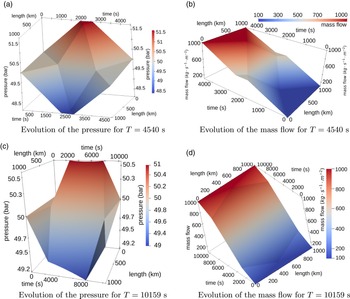
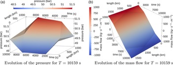
We first study the evolution of the pressure and flow across time and space, as shown in Figure 3. The triangular areas that appear flat are ${D_{\mathrm{I}}}$ on the right and ${D_{\mathrm{II}}}$ on the left. The main difference between the two different terminal times is the larger amplitude of the pressure, which varies around 50 bar, and a smoother transition of the mass flow from the initial value to the terminal one for $T=10,159$ s when compared to $T=4540$ s.

Figure 3.

Evolution of the pressure and mass flow.

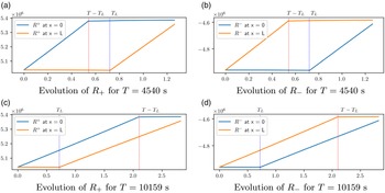
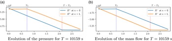
Now, we focus on the evolution of the Riemann invariants at the ends of the pipe as shown in Figure 4. First, remember that due to the finite propagation speed, the values of the Riemann invariants are fixed (or predetermined) by the initial and terminal states for some time. Namely, for $R_+$ this is the case at $x = 0$ for $t\in[T-T_L, T]$ , and at $x=L$ for $t\in [0, T_L]$ . For $R_-$ , this is the case at $x = 0$ for $t\in[0, T_L]$ , and at $x=L$ for $t\in [T-T_L, T]$ . There is a major difference in the control and behaviour depends on whether $T-T_L < T_L$ holds. If this is the case, then on the time interval $[T-T_L, T_L]$ both Riemann invariants are determined by the initial and terminal states. Hence, there is no ‘choice’ (in the sense of control input) of the Riemann invariants on that interval. This motivates the presentation of the numerical results with two terminal times: for the shorter time horizon $T = 4540\;\mathrm{s}$ , $T-T_L < T_L$ , whereas for the longer time horizon $T = 10,159\;\mathrm{s}$ this inequality does not hold. Two vertical lines, one for $t=T_L$ in blue, and one for $t=T-T_L$ in red, have been added to all the plots which depicts a time evolution.

Figure 4.

Evolution of the Riemann invariants at the end points.

In Figure 4(a) and (b), we see that $R_+$ at $x=0$ transitions from its initial value to the one at the start of the predetermined line segment in $[0, T-T_L]$ , and at $x=L$ the same appears in $[T_L, T]$ . For $R_-$ , we find the same phenomenon, with the values of x reversed. In Figure 4(c) and (d), we observe that the evolution of the Riemann invariants occurs at a less steep slope thanks to the longer duration $T-T_L$ of the transitions. Also, in the time interval $[T_L, T-T_L]$ , the values of both Riemann invariants can freely be selected, in contrast to the case $T = 4540\;\mathrm{s}$ , where only one component of R can be selected at any time. While all plots depicted in Figure 4 may appear to shown piecewise linear graphs only, this is just a visual effect due to the low friction and mass flow regime. Finally, note that the regularity of the Riemann invariants hinges on the choice of their values on the $I_{\mathrm{mid}}$ segment. Here, we use a simple linear interpolation. We expect that a smoother transition would also smoothen the values of $R_{\pm}$ at the end points. However, such an investigation is beyond the scope of this paper.

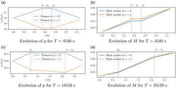
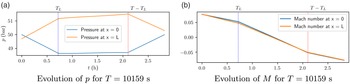
In Figure 5, the evolution of the pressure p and the Mach number M at the end points of the pipe are shown. The evolution of the pressure as shown in Figure 5(a) and (c) can be divided into three phases: first a change from the initial values to a plateau-like phase, and then a transition to the terminal state values. The duration of the first and third phase is $\min\{T_L, T-T_L\}$ for each, and the second one lasts for the remaining time. Note that the variation in pressure is much smaller in Figure 5(c) when compared to the one in Figure 5(a). For the Mach number M, the same behaviour with three phases is present. Now, the difference between Figure 5(b) and (d) is in the rate of change of the Mach number, with the extremal values being the same, respectively. In particular, remember that for $T = 4540\;\mathrm{s}$ , the control input is predetermined on $[T-T_L, T_L]$ . Hence, outside this time interval, the rate of change has to be larger in order to account not only for the reduction in terminal time, but also for this additional constraint.

Figure 5.

Evolution of the pressure p and Mach number M at the end points.

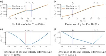
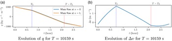
In Figure 6(a) and (b), the evolution of the mass flow at the end points is depicted. The behaviour is quite similar to the one for the Mach number in Figure 5(b) and (d).

Figure 6.

Difference in gas velocities $\Delta v\;:\!=\; v(\cdot, 0) - v(\cdot, L)$ between the end points.

Finally, in Figure 6(a) and (b), the difference $\Delta v$ in gas velocity at the end of the pipe is shown. The values depicted in Figure 6(a) drop more rapidly and remain relatively constant in the time interval $[T-T_L, T_L]$ , whereas in Figure 6(b), the change is comparable in all three time intervals.

Example 7.3. Let us now move on to the second scenario: a flow inversion in the pipe, from $q_0 = 1000\;\mathrm{Kg\,s}^{-1}\mathrm{m}^{-2}$ to $q_T = -1000\;\mathrm{Kg\,s}^{-1}\mathrm{m}^{-2}$ , while keeping a pressure of $p = 50\;\mathrm{bar}$ at $x = 0$ . The associated pressure profiles are given in Figure 7. The evolution of the pressure and mass flow rate are depicted in Figure 8. Given a terminal time much larger than $T_L$ , the flow reversal is rather smooth across the pipe, as one can see in Figure 8(b). In Figure 8(a), as expected, we observe that the pressure increases at $x=L$ and decreases at $x=0$ to induce the switch.

Figure 7.

Pressure profile in the pipe associated with the initial and terminal state, both being stationary.

Figure 8.

Evolution of the pressure and mass flow.

As for the previous numerical analysis, we first focus on the evolution of the Riemann invariants in Figure 9. The same three phase regime with $T-T_L > T_L$ is observed. The evolution of $R_\pm$ follows the same logic as before: outside of the predetermined values, the Riemann invariants evolve according to the values on $I_{\mathrm{mid}}$ propagated through the $R^{\mathrm{III}}$ and $R^{\mathrm{IV}}$ domains.

Figure 9.

Evolution of the Riemann invariants at the end points.

This yields the pressure and Mach number as shown in Figure 10. The main difference between the end points is the pressure, which evolves in a symmetric fashion between the end points of the pipe: a decrease (resp. increase) on $[0, T_L]$ followed by a plateau-like phase, and finally an increase (resp. decrease) on $[T-T_L]$ to the values given by the stationary solutions. Note how the pressure at $x=L$ transitions from a smaller value to a larger one at $x=0$ . The amplitude of the pressure remains small in this scenario. For the Mach number, in Figure 10(b), the difference between the end points remains small. The same can be stated about the evolution of the mass flow in Figure 11(a), where the difference appears even smaller. In Figure 11(b), the difference $\Delta v$ in gas velocity sheds some light on the difference between end points values.

Figure 10.

Evolution of the pressure p and Mach number M at the end points.

Figure 11.

Difference in gas velocities $\Delta v = v(\cdot, 0) - v(\cdot, L)$ between the end points.