Introduction
All species of sea turtles in Mexico are classified as at risk by both national and international organizations; in particular, the green turtle (Chelonia mydas) is classified as in danger of extinction by the Mexican Red List and as endangered by the IUCN Red List of Threatened Species (Seminoff, Reference Seminoff2004; NOM-059-SEMARNAT-2010, 2010; IUCN 2019). The life cycles of sea turtles are highly complex. These cycles take place over long periods of time and over great distances, spanning feeding to nesting sites, and are characterized by low growth rates and late sexual maturation. Being migratory animals, sea turtles are exposed to diverse environments during their development, which makes them vulnerable to abiotic factors that are influenced by anthropogenic activities, such as changes in ambient temperatures. Sea turtles present temperature-dependent sex determination (TSD). Nests with higher temperatures produce more females, while nests with lower temperatures produce more males (Saba et al., Reference Saba, Santidrián-Tomillo, Reina, Spotila, Musick, Evans and Paladino2007). As coastal temperatures rise, higher nest temperatures may put some sea turtle populations at risk as sex ratios may show a female bias. In addition to nest temperature, sea surface temperature (SST) is one of the most important abiotic factors affecting sea turtle development as SST is highly correlated with reproductive behaviour, reproductive performance and the probability of nesting between seasons (Mazaris et al., Reference Mazaris, Kornaraki, Matsinos and Margaritoulis2004; Saba et al., Reference Saba, Santidrián-Tomillo, Reina, Spotila, Musick, Evans and Paladino2007).
Sea turtles present sexual dimorphism in adulthood and not as juveniles. Differentiating between adult and juvenile sea turtles may be accomplished by comparing morphometric measurements, such as straight carapace length (SCL). For example, C. mydas individuals with SCLs less than 77.3 cm are considered to be immature turtles (Seminoff, Reference Seminoff2000). The technique proposed by Bolten (Reference Bolten, Eckert, Bjorndal, Abreu-Grobois and Donnelly1999) was used to measure total tail length (TTL), which was defined as the distance from the midline of the posterior margin of the plastron to the end of the tail following the curvature of the tail, and to differentiate between male and female adult sea turtles. Males develop a long and muscular tail (>20 cm) during puberty (Limpus & Reed, Reference Limpus, Reed, Grigg, Shrine and Ehmann1985; Wibbels et al., Reference Wibbels, Owens, Morris, Amoss and Witzell1987). Adult Chelonia mydas males can show TTLs in excess of 20 cm (Meylan et al., Reference Meylan, Davis and Meylan1994), but some large immature sea turtles have not yet developed large tails and thus may be mistaken for females based on TTL measurements (Wibbels, Reference Wibbels, Eckert, Bjorndal, Abreu-Grobois and Donnely2000). Using TTL measurements for this ontogenetic stage to sex turtles can often lead to the misidentification of individuals (Limpus & Reed, Reference Limpus, Reed, Grigg, Shrine and Ehmann1985; Wibbels et al., Reference Wibbels, Owens, Morris, Amoss and Witzell1987). Also, sexing sea turtles using only TTL measurements implicitly assumes that turtles with small TTLs are more likely to be females rather than immature individuals (Casale et al., Reference Casale, Freggi, Basso and Argano2005). Sexing immature sea turtles correctly often requires invasive and expensive methods, such as laparoscopy, gonad dissection, or testosterone level measurements. All of these methods imply surgical training and are difficult to perform in the field (Wibbels et al., Reference Wibbels, Owens, Morris, Amoss and Witzell1987). Of the available methods, sexing sea turtles using morphometric measurements is the least invasive and easiest to carry out; nevertheless, this method should be used carefully as immature males may be mistaken for small females (Limpus & Reed, Reference Limpus, Reed, Grigg, Shrine and Ehmann1985).
Differences in a few characteristics relating to ontogeny have been explained using mathematical models for different species (Bolten & Bjorndal, Reference Bolten and Bjorndal1992; Van Dam & Diez, Reference Van Dam and Diez1998; Bjorndal et al., Reference Bjorndal, Bolten and Chaloupka2000). Combining morphometric measurements with mathematical modelling is a straightforward and non-invasive approach to sex sea turtles regardless of ontogenetic stage and provides a more precise estimate of the sex ratio present in sea turtle populations. Marine turtles in foraging areas represent an important opportunity for such studies as both sexes and all stages of ontogeny are often present in these zones.
This study was performed in Bahía de los Ángeles (BLA), Baja California, Mexico, which is one of the principal foraging and resting areas for C. mydas in the Gulf of California (Seminoff et al., Reference Seminoff, Jones, Resendiz, Wallace and Chaloupka2003). Furthermore, green turtles in this area exhibit hibernation behaviour, as has been described for other geographic regions (Hochscheid et al., Reference Hochscheid, Bentivegna and Hays2005). To date, no sex predictor model that employs morphometric measurements exists for C. mydas from the Gulf of California. Adult and immature male and female C. mydas individuals are present in BLA, and thus sex ratio estimations are possible (Wibbels, Reference Wibbels, Eckert, Bjorndal, Abreu-Grobois and Donnely2000). An evaluation of the sex ratio present in this foraging area will provide an important framework to study the reproductive ecology of C. mydas populations. In addition, it will allow us to compare the sex ratio estimated by our model with the 1:1 sex ratio established by Fisher's evolutionary theory for adult males and females. The evaluation of this parameter will permit an estimation of C. mydas population growth and will be invaluable for developing effective management and conservation strategies for this species (Rees et al., Reference Rees, Alfaro-Shigueto, Barata, Bjorndal, Bolten, Borjeau, Broderick, Campbel, Cardona, Carreras, Casale, Ceriani, Dutton, Eguchi, Formia, Fuentes, Fuller, Girondot, Godfrey, Haman, Hart, Hays, Hochscheid, Kaska, Jensen, Mangel, Mortimer, Naro-Maciel, Ng, Nichols, Phillot, Reina, Revuelta, Scholfield, Seminoff, Shanker, Tomás, van de Merwe, Van Houtan, Vander Zander, Wallace, Wedemeyer-Strombel, Work and Godley2016) in BLA.
Materials and methods
Geographic area
Bahía de los Ángeles (BLA) is located on the eastern coast of the Baja California peninsula in Mexico at 28°58′N 113°33′W (WGS84). The bay is known for its high biological diversity and the presence of several foraging and hibernation areas for C. mydas (Seminoff et al., Reference Seminoff, Reséndiz-Hidalgo, de Reséndiz, NIchols, Todd-Jones, Daneman and Ezcurra2008; Hochscheid et al., Reference Hochscheid, Bentivegna and Hays2005). The climate of BLA is arid with an annual mean precipitation of 60.5 mm and high evaporation rate (Cavazos, Reference Cavazos, Daneman and Ezcurra2008). The annual mean sea surface temperature is 22.7 ± 1.4°C with a marked seasonality that oscillates between 14–15°C in January and February to 28–31°C in July and August (Seminoff, Reference Seminoff2000).
Data
Morphometric measurements of 529 C. mydas individuals were compiled from data collected from 1995–2005 provided by Jeffrey Seminoff (Seminoff et al., Reference Seminoff, Jones, Resendiz, Wallace and Chaloupka2003; Seminoff et al., unpublished data). The same morphometric data was collected from 2009–2012 by the governmental agency Comisión Nacional de Áreas Naturales Protegidas (CONANP). Sea turtles were sampled using entanglement nets measuring 100 × 8 m with a stretched mesh measurement of 50 cm. Nets were placed in different areas of BLA for 12 h and monitored at 2 h intervals. The morphometric measurements of straight carapace length (SCL, cm), curve carapace length (CCL, cm), straight carapace width (SCW, cm), curve carapace width (CCW, cm), plastron length (PL, cm), carapace depth (CD, cm), and total tail length (TTL, cm) were obtained as described by Bolten (Reference Bolten, Eckert, Bjorndal, Abreu-Grobois and Donnelly1999). Both SCL and CCL were measured from the anterior point at midline (nuchal scute) to the posterior tip of the supra caudals. The weight (W, kg) from captured turtles was taken prior to release. As with TTL, PL was considered to be a possible dimorphic variable as this has been found to be true for some aquatic turtles (Vega & Stayton, Reference Vega and Stayton2011; Lin et al., Reference Lin, Gaillard, Hu, Yang, Chen, Zhou, Xiao and Shi2017). Sex and ontogenetic stage were determined using SCL and TTL with the methodology explained below.
Statistical analysis
A principal component analysis (PCA) was employed to find morphometric variables that separated the sex or ontogenetic stage of individuals. With the variables obtained by multivariate methods, fitted allometric models were created between dimorphic variables (i.e. TTL, PL) and morphometric variables (i.e. SCL, CCL or CD) of the form Y = αX β, where Y represents a dimorphic variable and X the morphometric variable found via PCA for each stage of ontogeny. The Levenberg–Marquardt estimation method was used for model fitting and the software package STATISTICA (v. 8 StatSoft, Inc. Tulsa, OK) was used for all statistical analysis.
Results
Using the classic criteria for the determination of sex and maturity (adults, SCL > 77.3 cm; males, TTL > 20 cm) for C. mydas (N = 529) in BLA, we found that 44% (234 individuals) of the population was composed of immature organisms, while 43% (225 individuals) were females, and only 13% (70 individuals) were males. As such, the sex ratio estimation (F:M) was 3.2:1. The basic statistics for the sampled individuals are shown in Table 1.
Basic statistics for morphometric variables used in the principal component analysis and model fittings

SD, Standard Deviation.
All variables are measured in centimetres.
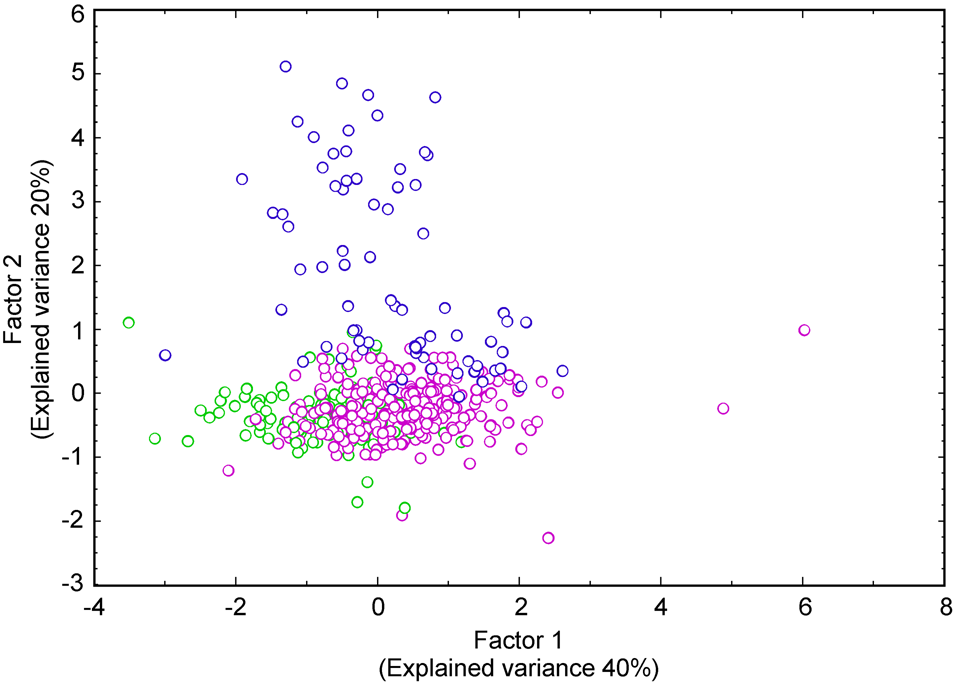
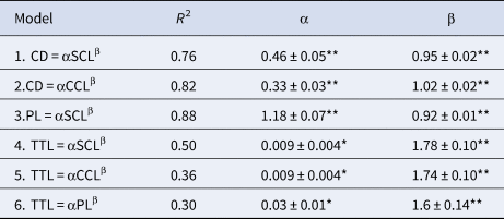
The PCA analysis that included all stages of ontogeny (immature and adult female and male individuals) extracted four principal components with 97% of the explained variance. Nevertheless, only the first two principal components separated the ontogenetic stages. The first component was mainly represented by a linear combination of SCL, CCL, PL and CD and describes 40% of the explained variance. The second principal component was represented principally by TTL with an explained variance of 20%. Figure 1 presents principal component 1 vs principal component 2 and clearly shows the separation of these stages. It is worth noting that the other components were omitted from future analyses as they did not separate individuals of different stages, which was the main purpose of the analysis. In Figure 1, some possible erroneous data were detected (i.e. individuals that could be erroneously sexed). For example, an individual sexed as male with SCL < 77.3 cm or TTL < 10 cm. These data were eliminated from further analyses to obtain a better fitted model. With the most important variables identified from the PCA, six allometric models were fitted with the aim of finding a relationship that unambiguously sexed C. mydas individuals. Table 2 summarizes the best allometric models between variables that fulfilled the requirements for the Levenberg–Marquardt fitting method and also contains the determination coefficient of each model, the estimated parameters with associated standard errors, and P-values. Normality and homoscedasticity of residuals were verified through a residual analysis for each model.
Main variables that separate individuals by sex and stage of ontogeny, found from the PCA. The first factor mainly characterized by SCL, CCL, CD and PL explains 40% of total variance. The second principal factor is mostly represented by TTL and explains 20% of the overall variance. Green, pink and blue dots represent un-sexed immatures, females and males respectively.

Fittings of allometric models using the most important variables found in the PCA, along with the determination coefficient (R 2), fitted parameters α and β with standard errors

*P < 0.05, **P < 0.001.
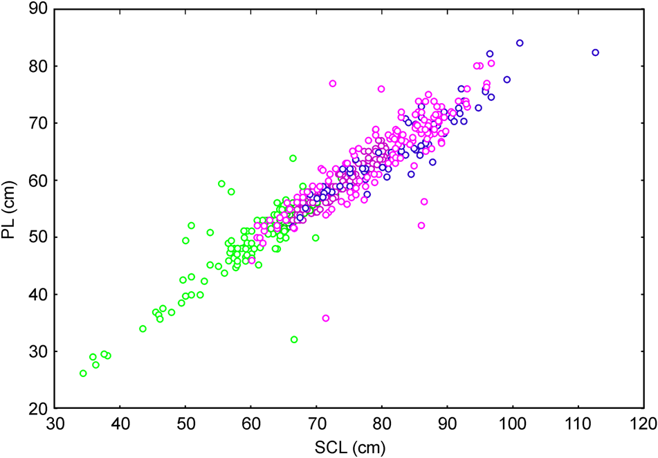
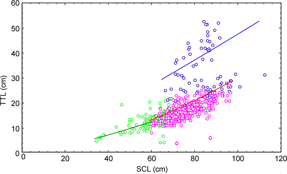
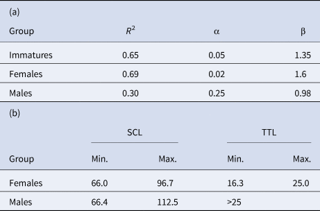
Even though the models that included PL and CD were deemed to be good, they were only able to separate adults from immature individuals. Therefore, the variables PL and CD were not good indicators for determining sex but excellent indicators of sexual maturity, as shown in Figure 2, which presents model 3 (PL = αSCLβ). The graph of model CD = αSCLβ presents a similar situation and was thus omitted. On the other hand, the best model that included TTL was model 4 (TTL = αSCLβ), which shows a clear separation of adult males and females as well as of the two ontogenetic stages (Table 2, Figure 3). In order to find reference values for the principal variables that were able to sex organisms unambiguously, model 4 was fitted separately to each subset of organisms (i.e. immature females and immature males). Table 3a presents the fitting results, while Table 3b presents the maximum and minimum values estimated for the fitting results for both males and females.
The fitting of PL = αSCLβ produced a high determination coefficient (R 2 = 0.88), but did not separate individuals by sex nonetheless, separated adults and immature in a well manner. Green, pink and blue dots represent un-sexed immatures, females and males respectively.

Fittings of model TTL = αSCLβ for each group separately. Green, pink and blue dots represent un-sexed immatures, females and males respectively.

(a) Fittings of the most representative model TTL = αSCLβ for females, males and immatures separately. (b) Reference values of TTL and SLC found from the fitted models Females and Males

As organisms were considered to be immature only if SCL < 77.3, it was possible to solve for SCL in the equation TTL = αSCLβ and set the resulting equations equal to each other for immature individuals and females and immature individuals and males using the fitted values for α and β from Table 3a. In this manner, we obtained two new equations relating immature individuals to females and immature individuals to males in terms of TTL. Then, by solving each equation for TTL, which was a dimorphic variable, we obtained an estimation of potentially immature males and females. That is, immature individuals could be considered potential females if
 $${\rm TTL} = e^{\lpar {1.6Ln\lpar {0.05} \rpar -1.35ln\lpar {0.02} \rpar } \rpar /\lpar {1.6-1.35} \rpar } = 7.04\comma \;$$
while individuals could be considered to be potential males if
 $${\rm TTL} = e^{\lpar {0.98ln\lpar {0.05} \rpar -1.35ln\lpar {0.25} \rpar } \rpar /\lpar {0.98-1.35} \rpar \rpar } = 17.8.\;$$
Therefore, immature individuals were considered to be potential females if TTL < 7.04 and potential males if 7.04 < TTL < 17.8.
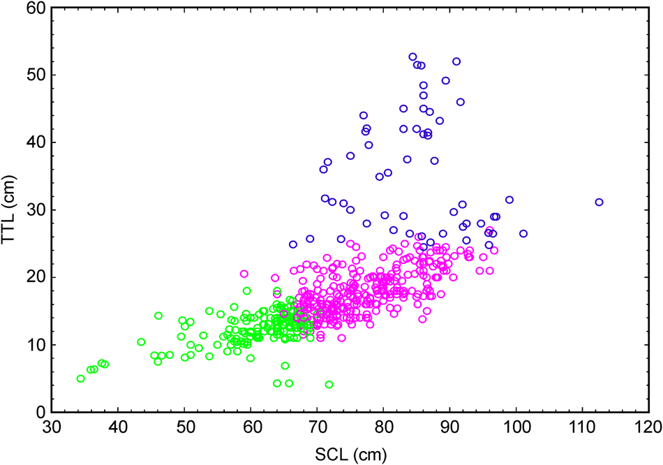
Taking these criteria into consideration, the results indicated that the immature population presented a 2.5:1 (F:M) ratio. Finally, by re-sexing the adults with the maximum and minimum values from Table 3b, a new estimation of the adult sex ratio was obtained, which was 5.1:1 (F:M) for this population. By plotting SCL vs TTL for re-sexed organisms, we observed a better separation of individuals depending on group (i.e. immature females or immature males; Figure 4).
SCL vs TTL for re-sexed individuals with values obtained from fitted models and Table 3. Green, pink and blue dots represent un-sexed immatures, females and males respectively. A clear separation of groups is observed.

Discussion
Mathematical models, in addition to requiring non-invasive methods, were useful for determining the reference values of the morphometric characteristics required to determine the sex of C. mydas individuals in our study site with great precision. We found that the mathematical relationship between SCL and TTL provided a straightforward method to sex both adult and immature C. mydas individuals.
Other authors have also found mathematical relationships between various morphometric characteristics in C. mydas. For example, Bolten & Bjorndal (Reference Bolten and Bjorndal1992) found a relationship between SCL growth rates and mean SCL values for immature organisms, while Bjorndal et al. (Reference Bjorndal, Bolten and Chaloupka2000) presented generalized additive models (GAMs) to relate specific SCL growth and body mass. In our study, PL was determined to be an important variable based on the results of the PCA (r = 0.79). The results of our models for C. mydas indicated that a maximum SCL value (65.5 cm), which is considered to be the size of C. mydas individuals near maturity in this region (Meylan et al., Reference Meylan, Meylan and Gray2011), corresponded to an estimated PL of ~53 cm. Therefore, if PL > 53 cm, the individual can be considered to be an adult, which is consistent with the maximum value for an immature individual proposed by other authors (Bolten & Bjorndal, Reference Bolten and Bjorndal1992; Grossman et al., Reference Grossman, Mendonca, Rodríguez da Costa and Bellini2007; Prior et al., Reference Prior, Booth and Limpus2015). Furthermore, Van Dam & Diez (Reference Van Dam and Diez1998) used an allometric model for Eretmochelys imbricata to evaluate the relationship between SCL and TTL and determined the classification ranges of these variables for immature individuals (20–60 cm, SCL; 5–13 cm, TTL), adult females (70–100 cm, SCL; 13–25 cm, TTL), and adult males (75–90 cm SCL; TTL > 25 cm). These results are consistent with the findings of our study and with the findings of Thomson et al. (Reference Thomson, Burkholder, Heithaus and Dill2009) who reported TTLs > 25 cm for adult C. mydas males. Rees et al. (Reference Rees, Margaritoulis, Newman, Riggall, Tsaros, Zbinden and Godley2013) studied Carretta caretta in Mediterranean waters and found that individuals with TTL > 6 cm were highly likely to be females, which was based on the tail measurements of nesting females. In our study, we did not have data of nesting females and thus could not compare our results to those of Rees et al. (2013). However, the average TTL for females in this study was 17 cm, which agrees with the findings of our models (Table 3b).
The reference values for SLC and TTL that were obtained by fitting allometric models allowed us to find possible measurement and sexing errors simply through the inspection of graphs and data, in addition to allowing us to successfully sex individuals of the sample population in any stage of ontogeny without using invasive methods. Data cleaning and model fitting allow for a precise estimation of the sex ratio, which is an important parameter needed to evaluate the success or dynamics of any given population. In this particular case, the initial estimation of the sex ratio (3.2:1, F:M) was biased toward females. These values are similar to those reported by Allen et al. (Reference Allen, Robbins, Eguchi, Owens, Meyla, Meylan, Kellar, Schwenter, Nollens, Leroux, Dutton and Seminoff2015) for the same species in a foraging area in San Diego, California (3.5:1, F:M). Once the erroneous data were corrected and the values for the adults presented in Table 3b were applied, the resulting sex ratio estimation was 5.1:1 (F:M) for adult organisms. Using the results of equations (1) and (2) for immature individuals, a sex ratio of 2.5:1 (F:M) was estimated. By grouping both stages of ontogeny, a sex ratio of 3.7:1 (F:M) for the entire population in the area was obtained. While similarly high values have been reported for immature green turtles in Malaysia (4:1, F:M) using data from laparoscopic examinations (Pilcher, Reference Pilcher2010) as well as in Australia (4.2:1, F:M; Limpus et al., Reference Limpus, Bell and Miller2009), these values are not congruent with Fisher's theory of population stability. The variation in both the sex proportion and ontogenetic structure through time could reflect ecosystem changes, which might be the result of a variety of factors, including climate change. This observed variation emphasizes the necessity of employing robust methods for both sexing and determining the ontogeny of individuals in order to better characterize the population structure of sea turtles in a given area.
This study has clearly shown a robust, non-invasive and simple alternative for sexing sea turtles in any stage of ontogeny. As with any other methodology, we are aware that some degree of uncertainty is associated with our methods, especially with regard to immature individuals. The addition of other dimorphic variables into our models, such as pre-cloacal length (PreCL, defined as the distance from the proximal to the cloaca), post-cloacal length (PostCL, defined as the distance from the cloaca to the tip of the tail), and some of the proportions of the morphometric measurements proposed by Casale et al. (Reference Casale, Freggi, Basso and Argano2005) for Caretta carretta, may be beneficial. Our initial observations for C. mydas regarding PreCL and PostCL suggest differences between females and males, but the data were insufficient for statistical analysis. However, these two new measurements could provide an even more robust determination of sex for this species. Also, it is very important to establish an estimation of male size at maturity for C. mydas as has been done for other sea turtle species (Casale et al., Reference Casale, Freggi, Basso and Argano2005; Ishihara & Kamezaki, Reference Ishihara and Kamezaki2011; Rees et al., Reference Rees, Margaritoulis, Newman, Riggall, Tsaros, Zbinden and Godley2013). Correlating these measurements with SCL and TTL could help us to refine sexing models for C. mydas in all stages of ontogeny. Finally, the models could also be calibrated with hormone concentrations or a similar characteristic to validate their robustness and applicability to other species, like the model developed by Shertzer et al. (Reference Shertzer, Avens, Braun McNeill, Goodman Hall and Harms2018) for C. caretta that employed morphometrics and testosterone data with Bayesian mixture models. This model was able to discriminate the sex of juvenile loggerheads of the Core and Pamlico Sounds in North Carolina, USA. The model obtained in this work should be tested in other C. mydas aggregation sites, such as Bahía Vizcaíno, Bahía Magdalena and Laguna Ojo de Liebre, which are located along the western coast of the Baja California peninsula, as well as in other sites in the Gulf of California, such as Cabo Pulmo (Koch et al., Reference Koch, Brooks and Nichols2006; Comisión Nacional de Áreas Naturales Protegidas, 2006).
Acknowledgements
The authors thank CONANP for providing the data from 2009–2012 and Jeffrey Seminoff who provided data from 1995–2005. We also thank Francisco Ponce for the fine graph and table work and Andrea Lievana-MacTavish and Emilio Godinez-Lazarini for English editing.