

1. Introduction
We live in a world that appears to be factual in the past and open in the future. The present represents the slim border between past and future where the so-far open future is concretized and transformed into the past. However, if we think of processes that are, in some way or the other, influenced by human agents this view is a simplifying stylization. The reason is that the past, in general, cannot unanimously be uniquely reconstructed, but needs an interpretation so that multiple possible reconstructions compete. And the future is not completely open, or arbitrary, but is more or less restricted by the present and the past.
To be sure, thinking about alternatively possible processes is not only reasonable for the future. In fact, taking the position of a past state in a ‘Gedankenexperiment’ – thought experiment – and looking to the (past) future from there may open a space of alternative possible processes to the factual process. Although these alternative processes have alternatively been possible, they are of course ‘counterfactual’ from the present perspective. The property of the present, or of a past, or future, state to have multiple possible futures will be characterized by the term ‘contingency’ in this article. It is important for the proper understanding of this term that it neither means that the future is a necessary result of the present and the past, nor that the future is completely open without any restrictions. In other words, contingency means that at any state of a processes in historical time which is influenced by human agents, there are certain degrees of freedom for the realization of the future states ‘between chance and necessity’.Reference Monod1 To analyse these degrees of freedom for the present state means to better understand what will come in the future, whereas to analyse them for a past state means to better understand whether the present state has been inevitable, or necessary, or whether it is just one of several possibilities that could have been realized.
Indeed, the use of the subjunctive in everyday communications shows how pervasive thinking in contingencies is in real life. Contingency thinking, or counterfactual thinking in the sense of ‘what if …’ (see Section 3 below), is illustrated in an impressive manner in poetry, stage plays and cinema movies. To start with the last group, think for instance of It’s a Wonderful Life (1956), Rashomon (1958) or Groundhog Day (1993). Jean Paul’s Konjekturalbiographie (1818), Max Frisch’s Biografie (1984), Robert Musil’s Der Mann ohne Eigenschaften (1930–1952) or Yasmin Reza’s Trois Versions de la Vie (2000) give examples of ‘contingent’ poetry and stage plays.
The article is organized in the following way. Section 2 provides the reader with the intuition of and first insights into our concept of contingency and causality in economic processes. Applications in the ‘counterfactual analysis’ and in the ‘contingency scenario analysis’ are described in Section 3. The formal contingency concept is developed in Section 4. The subsequent three sections show applications and extensions of our formalized contingency concept: the causality degree in Section 5, path dependence in Section 6, and the contingency proximity degree in the final section.
2. Contingency and causality in economic processes
Looking at the etymology and epistemology of the term ‘contingent’ one finds that it is derived from ‘contingere’ (literally ‘to coincide’, but also: to happen, to make possible) with its roots in the ancient Greek term ‘endechómenon’ (‘possible’, from Greek ‘endéchesthai’: to admit) used by Aristoteles in his opus ‘logic of modality’.2, Reference Janich and Lorenz3 There has been a broad epistemological debate on the understanding of ‘contingency’.Reference Becker-Freyseng4–Reference Lorenz11 We will apply here the widely accepted meaning of a contingent event as being ‘not impossible, but not necessary’.Reference Lehmann-Waffenschmidt, Fulda and Schwerin7, Reference Hoering12, Reference Wolters13
Let us look closer at an evolving socio-economic system (e.g. a national economy, or a firm). If no alternatives of the present state from the past state(s) are conceivable then the present state is in some sense necessary.Reference Lorenz14 Real world processes, however, in general are more complex.Reference Engels and Mittelstraß15, Reference Mainzer16 Thus, if there are alternatives of the present state, the actual present is only a possible, but not necessary consequence from the past. Then the present state is contingent.Reference Ortmann17 For each one of the contingently possible successor states of the past state a reasonable explanation – which may, but need not necessarily, employ stochastic influences – is possible. It is a particular feature of our contingency concept that it does not need probabilities if there is no information about probabilities, but it can integrate stochastics if probabilities are available.
How the final selection of one successor state from the set of alternatively possible successor states does work is, however, beyond our analysis: the fact that at a time only one alternative state of the open-loop evolving system under consideration can be realized does not imply that there must have been a determinismReference Hargreaves-Heap and Hollis18 – the factual state can be selected from a set of possible alternatives. Indeed, there is a strand in economics, i.e. the literature on evolutionary economics, that deals with the openness of economic processes.Reference Dopfer19–Reference Witt21 The evolutionary economics approach, in particular gives up the teleological idea of equilibrium.Reference Lehmann-Waffenschmidt, Fulda and Schwerin7, Reference Spaemann and Löw22, Reference Shackle23.
It is natural to ask for the causality relationship between past states and the present state. Causality Reference Pearl24–Reference Stegmüller26 in its strict sense means a close relation between observable causes and consequences, and it can correctly be explained how the causes lead to the consequences. This opens the whole epistemological discussion on necessary and/or sufficient causes (e.g. the debate on the so-called INUS conditions). In this approach, however, we will go in another direction: Throughout the whole article we do not understand ‘causality’ in the sense of a chain explaining effects from causing factors. Given a system evolving over time in an open-loop way, i.e. with degrees of freedom generated by human actions, we will understand the term ‘causality’ in a modified way: It denotes the gradually measurable intertemporal relationship of any two states of the evolution of observable characteristics (e.g. the central bank interest rate of the European Currency Union) of the evolving system under consideration (e.g. the economy of the European Currency Union).
To speak in terms of the example: the present central bank interest rate of the European Currency Union L 0 is of course not caused by its value L −1 a month earlier. In fact, the causal interrelationship between L 0 and L −1 is explained by a sequence of decisions by the central bank board during the last month, and the board had to make these decisions by its assessment of the macroeconomic and political pros and cons of changing, or maintaining, the interest rate L −1. We will speak of a (gradually measurable) causal interrelationship between L 0 and L −1 in the following sense (not taking into account the fact that former values of the interest rate indeed have an impact on its present value). The relevant entities of our consideration are the values of the interest rate as a result of the reasoning processes by the board, not the reasoning processes themselves. In a specific historical situation, several alternatives could be possible for L 0 – say, for instance, the unchanged value L −1, or a raise by 0.1 or maximally by 0.2. Each one of these three alternatives L 01, L 02, L 03 is linked to L −1 by a certain set of reasons favouring this alternative. Thus, the causes for the decision L 0i, i ∈{1, 2, 3} explain the causality between L −1 and its successor value in the traditional sense. However, for our ‘derivative’ understanding of causality, which emphasizes the diachronical sequence of alternatively possible values, the resulting value of L 0 is the relevant ‘consequence’. Causality in our understanding is between chance and necessity: The weaker the causal relationship between L −1 and L 0, the more alternatives can be reached from L −1 at date t 0. It would be maximal if the value of L 0 were to be uniquely determined.
3. Applications of the contingency approach in counterfactual analysis and contingency scenario analysis
A wide field of applications of contingency in our sense is counterfactual thinking Reference Ortmann17, Reference Cowan and Foray27–Reference Weber34. A ‘counterfactual’ is an ex-post constructed non-factual (essential) characteristic of a factual state Ei at time ti, or of a subperiod, of a historical process. A counterfactual can (1) have the property that there are plausible and convincing reasons for it in the factual historical context. This means that the construction of the counterfactual must be historically plausible, and the counterfactual analysis shows whether historically possible different processes with different results could have resulted from the counterfactual. For instance, the assassination of the Habsburg heir to the throne in Sarajevo in 1918 could have been prevented if the prince’s driver had not chosen the wrong route that day. The answer from counterfactual history analysis to the essential question of whether the First World War could have been prevented by that, however, is ‘no’.
Conversely, a counterfactual can be (2) an unrealistic assumption. Then the counterfactual history analysis does not show realistic alternatives to the factual historical course, but it can clarify whether the ‘factual’, which has been substituted by the counterfactual, had a truly causal effect on the outcome of the historical process. This was the procedure taken by the later Nobel laureate (1995) Robert Fogel (and co-authors) in the 1960s in their investigation of the question whether the development of the railway system in the USA was necessary for the economic take-off in the second half of the 19th century.Reference Fogel33 In fact, the answer was ‘no’. Fogel could show by a quantitative ‘Kliometric’ analysis – a mixture of history and quantitative econometric methods – that the factual railway system could have been substituted by extending the conventional transport techniques in order to achieve the same economic growth in the USA experienced with the factual developing railway system.
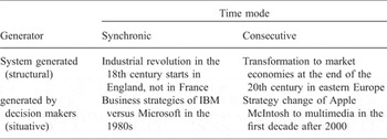
A usual objection against counterfactual reasoning is the following: if we could change one, or several, conditions in a historical process, or event, in a ‘Gedankenexperiment’ – how can we assume in a ‘ceteris paribus manner’ that all other conditions would remain constant? This objection can be neutralized by at least two counter-objections: (1) counterfactual arguing is just a method to systematically explore causality relations in historical processes, not to generate a new reality in the past or present.Reference Cowan and Foray27–Reference Weber34 (2) A counterfactual analysis may mutate into an ‘alternative factual analysis’ where the objection from above becomes irrelevant because the ‘counterfactual’ comparative process is a factual alternative, not merely a virtual one. In fact, there are historical consecutive, or synchronic, realizations of alternative process variants. Examples are given in Table 1.
Regimes of counterfactual analysis with examples

Table 1 shows a 2 × 2 matrix that represents an organization of counterfactual analysis on two levels – on the level of time, on the one hand – i.e. we distinguish between synchronic or consecutive alternative process realizations – and on the level of the ‘generator’ on the other hand – i.e. we distinguish between (an) identifiable personal decision maker(s) and a system. This results in four possible ‘regimes’ where counterfactual analysis can be applied. (1) Why did the industrial revolution in the 18th century start in England, not in France? A comparative (alternative factual) analysis of these two synchronic processes faces the problem that the causes cannot be found in identifiable (group) decisions, but are system generated (e.g. a decentralized market-oriented economy in England versus a centralized state-oriented economy in France, etc). (2) In contrast, decision makers are identifiable in the case of the business strategies of IBM and of Microsoft in the 1980s. Microsoft focused on personal computers, IBM did not – with the well-known consequence that IBM fell behind its competitors in the hardware industry, and Microsoft became a giant in the software industry. (3) Not synchronic, but consecutive, are the realizations of alternatives by identifiable decision makers, e.g. in the strategy change of Apple McIntosh from a pure computer producer to a multi-media supplier in the first decade of the 2000s. (4) The transformation to market economies at the end of the 20th century in the countries of eastern Europe gives an example of the consecutive realization of system-generated strategies.
There is a long tradition of counterfactual historyReference Wenzlhuemer28, Reference Demandt30, Reference Weber34 starting with ancient Greek and Latin authors, such as Thukydides and Titus Livius. Other names for counterfactual history are uchronique (‘no time’) in analogy to utopia (‘no space’), or alternative, as if, conjectural, might-have-been, parallel, quasi, unhappened, or virtual history. Later, one finds counterfactual thinking in the writings of Scottish moral philosophers in the 18th century. Heinrich Heine (Herrmann’s Battle), Max Weber (Battle of Marathon),Reference Weber34 Arnold Toynbee (Alexander the Great), and Winston Churchill (‘counter-counter-history’ on the battle of Gettysberg) wrote counterfactual history essays. Actual authors of counterfactual history can, for instance, be found in Ref. Reference Wenzlhuemer28, well-known authors besides Fogel of the New Economic History, or Kliometrics approach, are Crafts, Landes and McClelland. A particular interest on counterfactual thinking and arguing can be found in jurisprudence.Reference Slembeck35
So far, we have considered an ex-post analysis of contingency and causality. The question remains, however, how the contingency approach can be utilized for an ex-ante analysis, and what the differences to conventional scenario analysis are. Transforming the described counterfactual ex-post application of our contingency approach to the future, both the alternative possible states and the possible connections between alternative possible states of proximate points in time have to be predicted, not just reconstructed from historical knowledge. To be sure, this makes the analysis more speculative – which, nevertheless, applies to every kind of predictive analysis – and this will be the more disputable the larger is the distance to the present – analogous to the counterfactual ex-post application.
The ex-ante application of our contingency approach has a twofold advantage over conventional scenario analysis. First, scenario analysis usually does not model multiple possible connections between multiple possible states at different points in time. And second, from the perspective of one of the modelled future possible states in an ex-ante application of our contingency approach the analyst can apply the ex-post counterfactual application of the contingency approach. Thus, the whole analysis is applicable to this ‘virtual’ ex-post analysis, which is possible in the true ex-post case. In particular, one can pre-analyse possible responsibilities of the relevant decision makers for later outcomes in more detail than in a scenario analysis without multiple possible alternatives.
4. The formal contingency concept
We now proceed to the formalization of our contingency approach.Reference Lehmann-Waffenschmidt36 The leading idea is to transform the definition of a contingent event E of an evolving system as ‘not impossible, but also not necessary’ into a graph theoretical context. That means that, in the first step, an event E at time t will be modelled as an element of an appropriate set of alternative possible events at this point in time. In the next step, the elapsing time is integrated by connecting an event, or state, Et at time t by edges with those states E jt + 1 at time t + 1 which are possibly reachable from Et. In this way, a time directed ‘contingency graph’ is generated that reflects the possible alternative states of the evolving system at any time t as well as the possible evolution from a certain state to possible states at the next point of the time axis. An evolutionary process is represented as a path (Et, Et + 1, …) in a contingency graph.
In general, a contingency graph does not have the property to be a cycle-free ‘tree’ since it may well contain cycles. A cycle means that two, or more, evolutionary processes, i.e. paths, in the contingency tree at a certain state in the future may converge.
The following definitions fix these ideas.
Definition: An evolving system is characterized by a vector, or trajectory, (α 1t, …, αmt) ∈ Θ, t = 1, 2, 3, … of time-indexed characterizing parameters α 1, …, αm in the space of all admissible states Θ. A state of the evolving system at date t 0 is denoted by Et 0 = (α 1t 0, …, αmt 0).
The time discrete notation is not restrictive. In fact, our whole analysis could be generalized to the case of a continuous time parameter. The system characterizing parameters αi can be, but need not be (real) numbers. In our following two-dimensional graphical illustrations we symbolize the space Θ of all admissible states by the ordinate axis, whereas the abscissa denotes the time axis.
Definition: A contingency graph Γ is a directed di-graph, i.e. a time-directed graph that consists of two classes of elements – nodes, or states, and (connecting) edges – and may contain cycles. Γ represents, first, the possible states (nodes) of an evolving socio-economic system at any time and, second, the possible system evolutions by the set of edges connecting alternatively possible successive states in Γ.
Definition: A process in a contingency graph Γ is formalized as a path π, i.e. a finite, or infinite sequence of states (Ei ,Ei + 1, Ei + 2, …), or (Ei, Ei + 1, …, Ei +n), starting at time ti (and ending at ti +n in the finite case). Thus, a path is a selection of a unique states at each point in time from time ti on (until ti +n) in Γ, which are connected by edges in Γ.
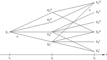
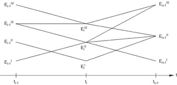
The contingency graph Γ reflects the contingency structure of π ∈ Γ (Figure 1). Γ can have a unique initial state as in Figure 1 or a multiple set of possible initial states as in Figure 2 (at time ti − 1).
Example of a contingency graph with a unique initial point E 1 and a path π.

Contingency graph with multiple possible initial points at time ti − 1.

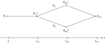
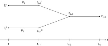
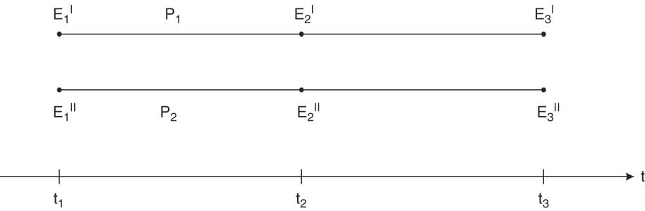
Looking more closely at the structural patterns of contingency graphs from the perspective of convergence and divergence we can distinguish four elementary patterns – see Figures 3 to 6.
Structural pattern 1: bifurcation without later convergence.

Structural pattern 2: bifurcation with later convergence (equifinality I) (e.g. convergence hypothesis about the convergence of poor and rich countries’ growth rate of neoclassical new growth theory).

Structural pattern 3: convergence with different initial points (equifinality II, e.g. technological lock-in processesReference Arthur37).

Structural pattern 4: Continual divergence with different initial points (e.g. factual persistent growth disparity between rich and poor countries).
Now we formalize the idea of progradeness and retrogradeness. In the first step, both concepts will be formalized for a state as an element of a path, in the second step we will formalize the ideas of prograde and retrograde alternative sets of an event.
Definition: A state Ei of a path π = (E 1,…, Ei − 1, Ei, Ei + 1, …) in Γ is contingent if besides Ei there is at least one more state E ji at time ti in Γ, which is a possible successor of Ei − 1. It is contingent in the retrograde sense if besides Ei − 1 there is at least one more state at time ti − 1 in Γ which is a possible precursor of Ei. Finally, Ei is contingent in the prograde sense if besides Ei + 1 there is at least one more state at time ti + 1 in Γ which is a possible successor of Ei.
We start with the definitions of prograde and retrograde alternative sets of an event in the case of proximate points in time. The expression ‘Ei can be reached from Ei − 1’ means that there is a connecting edge between Ei − 1 and Ei in the contingency graph.
Definition: The 1-prograde alternative set Ξi + 1P(Ei) of a state Ei of Γ contains all possible states of the contingency graph Γ at time ti + 1 which may be reached in Γ from state Ei.
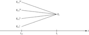
Definition: The 1-retrograde alternative set Ξi − 1R(Ei) of a stated Ei of Γ contains all possible states of the contingency graph at time ti −1 from which Ei can be reached.
Note that the superscripts ‘P’ and ‘R’ are not really necessary from a logical point of view since it is clear from the subindex of Ξ whether we deal with a prograde or with a retrograde alternative set. We will, however, keep to them throughout this presentation to provide a better intuition.
The next definition transfers the notion of the alternative set to a static point of view.
Definition: The set of alternatives, or the contingency set, Ξi at time ti contains all possible states of the contingency graph at time ti, i.e. all states that may been reached at time ti from some state of the contingency graph at time ti − 1. (Or to reformulate it in a recursive way: Ξi is the union of all 1-prograde alternative sets Ξi(Ei − 1) of all states from Ξi − 1.)
Returning to the evolutionary point of view we are going to define prograde and retrograde alternative sets of any event in the generalized sense for non-proximate points in time.
Definition: The m-prograde alternative set Ξi +m P(Ei) of Ei contains all possible states of the contingency graph Γ at time ti +m which may be reached from the state Ei in Γ (m > 0).
Definition: The n-retrograde alternative set Ξi − n R(Ei) of Ei contains all possible states of the contingency graph Γ at time ti −n from which the state Ei may be reached in Γ (n > 0).
5. The causality degree
In this section we will provide an operational formalization of the idea of gradual causality. To be more precise we are going to construct a causality degree that gradually measures causality relations between any two diachronical states of a generator system.
To formalize the notion of gradual causality with the help of our contingency approach we first have to differentiate between retrogradeness and progradeness. Let a contingency graph Γ, a path π, and states Ei − 1, Ei and Ei + 1 in π be given. In the most simple case of prograde causality we ask whether the state Ei is a necessary, or a weak or a strong cause for the succeeding state Ei + 1, i.e. whether Ei + 1 is a weak, or strong consequence of its precursor Ei. Or in other words: could also other states Ei + 1g ≠ Ei + 1 of Γ at time ti + 1 succeed Ei? Conversely, in the most simple case of retrograde causality we ask whether Ei is necessarily, weakly or strongly determined by Ei − 1, or in other words: could there have been different states Ei − 1j ≠ Ei − 1 in Γ precursors of Ei?
To be sure, in the case of proximate states Ei − 1, Ei and Ei + 1 these questions amount to a counting of elements of the prograde, or retrograde, alternative sets of Ei. But in the general cases of non-proximate states Ei −m, Ei and Ei +n simple counting of elements of the prograde, or retrograde, alternative sets will not be sufficient, but we will have to count paths and to form suitable quotients.
Let us start with the exact definition of a gradual measure of causality in the case of proximate states Ei and Ei + 1 (prograde case) and proximate states Ei − 1 and Ei (retrograde case).
Definition: The prograde degree of causality of proximate states Ei and Ei + 1, C PEi →Ei + 1, is defined by the inverse of the number of elements in the prograde alternative set Ξi + 1(Ei), or formally:

Definition: The retrograde degree of causality of proximate states Ei and Ei − 1, C REi →Ei − 1, is defined by the inverse of the number of elements in the retrograde alternative set Ξi − 1(Ei), or formally:

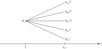
Figures 7 and 8 above provide an illustration for these definitions.
Example of a 1-prograde alternative set.

Example of a 1-retrograde alternative set.

To generalize these definitions to the general cases of non-proximate states Ei −m, Ei and Ei +n let us first provide the reader with some intuitive considerations. To measure the prograde causality relationship between a state Ei and a later state Ei +n in a gradual way: count the number of all connecting paths between the state Ei and Ei +n in Γ and put it into relation with the number of all alternatively possible paths in Γ between Ei and any state of Γ at time ti + n.
Analogously for gradually measuring the retrograde causality between Ei −n and Ei count the number of all connecting paths between the state Ei − n and Ei in Γ and put it into relation with the number of all alternatively possible paths in Γ between any state at time ti − n and Ei.
Let us now formalize this preparatory intuitive considerations.
Definition: If there exists at least one path connecting two arbitrarily chosen states Ei and Ei + n in Γ, the generalized prograde causality degree between Ei and Ei + n (n > 0), C PEi →Ei + n, is the quotient of the number v of connecting paths between the state Ei and the later state Ei + n in Γ (numerator) and the number w of all alternatively possible paths in Γ between Ei and any state at time ti + n (denominator). C PEi →Ei + n = v/w.
Analogously, we define as follows for the retrograde causality degree between Ei −m and Ei.
Definition: If there exists at least one path connecting two arbitrarily chosen states Ei −m and Ei in Γ the generalized retrograde causality degree between Ei and Ei −m (m > 0), C REi →Ei − m, is the quotient of the number y of all connecting paths between the states Ei − m and Ei in Γ (numerator) and the number z of all alternatively possible paths in Γ between any state at time ti − m and Ei (denominator). Thus, C REi →Ei − m = y/z.
Obviously, the retrograde causality degree between Ei and Ei −m equals 1 if Ei is the unique possible state at time ti, i.e. if Ξi is a singleton.
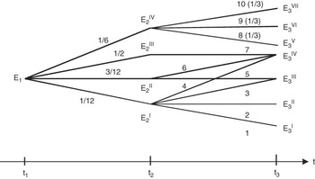
Figures 1 and 2 give an illustration of the definitions: in Figure 1, C PE 1→E 3III = 3/11; C PE 1→E 3I = 2/11. In Figure 2, C REi + 1II→Ei − 1IV = 1/5 ≠ C PEi − 1IV→Ei + 1II = 1/2.
Having reached this point the question arises for the relationship of our conceptualization and formalization of contingency and causality in processes with the probability approach. To be more precise let us put it into the two following questions.
1. Can additional information about probabilities of all or of some edges be integrated into the contingency approach?
2. Is the prograde and/or the retrograde causality degree the same as a conditional probability?
To anticipate the results of the analysis of these two questions, the answer to question 1 is ‘yes’ and to question 2 ‘no’. After that we will finish this section with a summary of the merits and advantages of the contingency approach in comparison with the probability approach.
To tackle the first question from above we will show that a ‘probability extension’ of the contingency approach is no problem. If probability weights of edges are given, the causality degree has to be calculated accordingly by weighted sums instead of unweighted sums as described in the definitions above. The definitions of causality degrees presented before are from a purely formal perspective a special case, namely the special case of an equal probability distribution on the alternatives of any prograde alternative set at any state. To be sure, however, from the perspective of lacking, or costly, information on probabilities of alternatives this case is the more general one.
To extend the definitions to the formally more general case of non-equally distributed probabilities of the alternatives, we have to introduce the notion of the probability weight of a process π first.
Definition: A path π = (Ei, Ei + 1, …, Ei +n) in Γ with n−1 edges ki, …, ki +n − 1, n > 0, has the probability weight
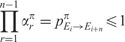
where αr π = probability of edge kr of π in Γ.
Obviously, the probability weight of a path is per definition the same as the conditional probability to reach Ei +n by π when starting in Ei.
Now we start with a first step towards a probability extension of our contingency approach.
Definition:The prograde probability weighted causality degree of type A of Ei and Ei +n, n > 0 is defined by
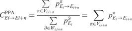
Vi,i +n is the set of all processes π in Γ which connect Ei and Ei
+
n. Wi,i
+
n is the set of all processes θ in Γ which start at state Ei and end in some state at time i + n.
Clearly, Vi ,i +n ⊆ Wi ,i +n, and the denominator equals 1. Thus 0 ⩽ C PPAEi →Ei +n ⩽ 1 is the conditional probability to reach Ei +n from Ei in Γ.
Since the denominator of the formal representation of C PPAEi →Ei +n equals 1, 0 ⩽ C PPAEi →Ei +n ⩽ 1 and C PPAEi →Ei +n is identical to the conditional probability to reach Ei +n from Ei in Γ. Nevertheless, the prograde probability weighted causality degree of type A is not substitutable by the conditional probability. We can see from the example of Figure 9, which summarizes all aspects of comparing the conditional probability, the not-probability weighted prograde causality degree, and the prograde probability weighted causality degree of type A.
Probability weighted contingency graph.

Figure 9 shows a subgraph Γ′ of the complete contingency graph Γ, which is not represented in figure. Γ′ starts at the present, time t 1, in the present state, E 1, and is restricted to nodes and edges from Γ that may be realized when starting from E 1. Let us look at E 1 and E 3VI.
1. The conditional probability to reach E 3VI from E 1: 1/6 × 1/3 = 1/18.
2. The Prograde probability weighted causality degree of type A C PPAEi →Ei +n of E 1 and E 3VI= 1/6 × 1/3 = 1/18 = conditional probability.
3. The not-probability weighted prograde causality degree C PE 1→E 3VI = 1/10 ≠ 1/18 = conditional probability.
4. Let the probabilities at all edges of Γ′ be equally distributed: Conditional probability = 1/4 × 1/3 = 1/12 = prograde probability weighted causality degree of type A C PPAEi →Ei +n = 1/12 ≠ not-probability weighted prograde causality degree C PE 1→E 3VI = 1/10.
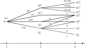
So far, our understanding of the subgraph Γ′ of Γ is that all possible paths start from the unique present state E 1. But looking at Γ′ as embedded in Γ leads to the insight that the present state E 1 of the subgraph Γ′ has a history in Γ so that there are a number of possible alternatives of E 1 at t 1 in Γ. Accordingly, we assume that E 1 is realized in Γ at time t 1 with probability α 1 (0 ⩽ α 1 ⩽ 1).
Definition: The prograde probability weighted causality degree of type B of Ei and Ei
+
n is given by

Vi, i +n is the set of all processes π in Γ that connect Ei and Ei +n. Wi,i +n is the set of all processes θ in Γ that start at state Ei and end in some state at time i + n. 0 ⩽ αi ⩽ 1 is the conditional probability that Ei is realized in Γ′ at time ti.
Clearly, Vi,i +n ⊆ Wi,i +n, and again the denominator equals 1. But 0 ⩽ C PPBEi →Ei + n ⩽ 1 is not necessarily identical with the conditional probability to reach Ei + n from Ei in Γ′ as we will see in the example of Figure 10, is identical to Figure 9 except for the new probability characterization of the initial state E 1.
Probability weighted contingency graph with probability weighted initial state E 1.

In the example of Figure 10, E 1 is realized in the complete contingency graph Γ with probability α 1 = 1/5. Not surprisingly, the prograde probability weighted causality degree of type B of Ei and Ei + n C PPB = 1/5 × 1/6 × 1/3 = 1/90 does not equal 1/18 = conditional probability.
Definition: The retrograde probability weighted causality degree of Ei +n and Ei is defined in the following way:
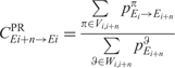
Vi,i +n is the set of all paths π in Γ that connect Ei and Ei +n. Wi,i +n is the set of all paths θ in Γ that start at a state at time i and end in state Ei +n.
Clearly, Vi,i +n ⊆ Wi,i + n, and 0 ⩽ C PREi+n→Ei ⩽ 1. From the definition of C PREi+n→Ei, it is furthermore clear that it is not identical with a conditional probability since the concept of conditional probability is not applicable to the concept of the retrograde probability weighted causality degree.
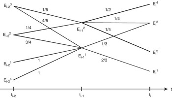
Let us calculate the retrograde probability weighted causality degree of Ei 3 and E (i − 2)3 from the example of Figure 11:

Retrograde probability weighted causality degree.

On the other hand the unweighted retrograde degree of causality

Let us summarize the merits and advantages of the contingency approach in comparison with the standard probability approach:
• The contingency approach and the standard probability theory approach have different origins and aims (for a comprehensive survey on modern probability and statistical theory see, for example, Refs Reference Pearl24 and Reference Hoover25). The contingency approach neither needs probabilities related to random samples and statistical universes, or populations, nor subjective probabilities. Nevertheless, the contingency approach can be extended by probabilities as we have shown before. The probability extension of the contingency approach cannot be reduced to standard conditional probabilities.
• Standard probability theory analyses dependencies and correlations of observed phenomena, not causalities in the sense of causing factors. Consequently, the standard probability theory approach is liable to the ‘correlation trap’, or even worse, to the ‘post hoc ergo propter hoc’-trap.
• In contrast to the standard probability approach, the contingency approach analyses causal relations between diachronical states in a gradual way and is differentiated with respect to progradeness and retrogradeness, i.e. with respect to cause or consequence.
• A contingent process is not a random realization from a statistical universe (population), but can ex-post be reconstructed in a reasonable way as a plausibly explicable sequence of states and transitions.
6. Path dependence and contingency
A contingency graph Γ need not necessarily be passable through all edges of all states, or nodes, independently of the history of the process under consideration. In fact, real processes often show a property called ‘path dependency’, which means that some states of the process are more or less predetermined by the previous history of the process.Reference Arthur37 To make it more precise, path dependencies in a path π in Γ reduce the degrees of freedom of the underlying process to progress on particular edges from particular nodes of π. In other words a contingency graph Γ in general is not of the ‘water flow model type’, but rather of the ‘rail switch model type’. Figure 12 shows a contingency graph Γ with a path dependency at E 3III: E 4III can only be reached from E 3III when E 3III has been reached from E 2IV or from E 2II, not E 2I (dotted lines in Figure 12). In addition, E 4I and E 4II can only be reached from E 3III when E 3III had been reached from E 2I, not from E 2II or E 2IV (broken lines in Figure 12).
A contingency graph with path dependencies.

Path dependency can be incorporated into our formal contingency model in both cases of prograde and of retrograde contingency. To start with the definition of prograde contingency with path dependency, let us again start first with the special case of a 1-prograde alternative set and then proceed to the general case of an m-prograde alternative set of a state Ei of a path with path dependency. In the following definitions we will generally take the view that a path dependency originates at a certain state of a process and remains active from that state over time until it disappears at a subsequent state. Naturally, prograde and retrograde alternative sets of a state Ei are in case of path dependency subsets of the ‘unconstrained’ (non-path dependent) alternative sets.
For all following definitions in this section let a contingency graph Γ, a path π = (E 1, E 2, …, Ei, …, En, En + 1, En + 2, …) in Γ be given.
Generally speaking, the 1-prograde alternative set of Ei with path dependency Ξi + 1Ppd in Γ is not only dependent on Ei as in the standard unconstrained case, but also depends on the k past states of Ei in Γ. More precisely:
Definition: The 1-prograde alternative set of Ei with path dependencies is denoted by Ξi + 1Ppd(Ei; Ei − 1, Ei − 2, …, E 1).
In the general case of an m-prograde alternative set of a state Ei with path dependency we notice that the path dependency, in general, has originated at a state Ei −k and is still valid for the m future states of the path from state Ei.
Definition: The m-prograde alternative set of Ei with path dependency is denoted by Ξi +m Ppd (Ei; Ei − 1, Ei − 2, …, E 1; Ei + 1, …, Ei +m).
Now let us proceed to retrograde alternative sets. Let us again start first with the special case of a 1-retrograde alternative set and then proceed to the general case of an m-retrograde alternative set of a state Ei with path dependency. To be sure, from the notion of path dependency, unconstrained 1-retrograde alternative sets are 1-retrograde alternative sets with path dependency. Thus, we can immediately proceed to the general definition of an m-retrograde alternative set of Ei with path dependency. Before providing the reader with the precise definition we first should make clear what an m-retrograde alternative set of Ei with path dependency should be.
Following the intuitive idea of a retrograde alternative set, an m-retrograde alternative set of Ei with path dependency Ξ(i −m )Rpd(Ei) is a subset of the standard alternative set Ξi − m R of Ei − m of π in Γ, which in fact shows a double path dependency property: (1) Ξ(i −m )Rpd(Ei) itself might be a prograde alternative set with ‘inherited’ path dependencies that originated at states previous to the state Ei − m in π, and (2) for any state E j(i − m ) of Ξ(i − m )Rpd(Ei) the state Ei must be an element of the m-prograde alternative set at time i = (i − m) + m with path dependency Ξ(i − m ) +m Rpd(E j(i − m ), E j(i − m )−1, …, E j(i − m )−k; E j(i − m )+1, …, E j(i −m )+m )). Property (2) means that Ξ(i − m )Rpd(Ei) not only depends on path dependencies having originated from states previous to the state Ei − m in π, but also depends on path dependencies in π arising between times (i − m) and i. Thus, the formal definition of Ξ(i − m )Rpd(Ei) refers to the definition of an m-prograde alternative set with path dependency. To make the formal notion of an m-retrograde alternative set more comprehensible we omit aspect (1) from above. This means we consider time ti −m as the initial time of the contingency graph, all path dependencies resulting from the past before ti −m are given as a ‘black box’.
Definition: The m-retrograde alternative set of Ei (m ⩽ i) with path dependency is given by the set Ξ(i − m )Rpd(Ei): = {E j(i −m ) ∈ Ξi − m|Ei ∈ Ξ(i − m ) +m Ppd[E j(i − m ); E 1(i − m )+1, …, E m(i − m )+m )]}.
To give an example, in Figure 12 the m-retrograde alternative set Ξ(4 − 2)Rpd(E4III) of E4III is {E2II, E2IV}, not {E2I, E2II, E2IV}.
7. The contingency proximity degree
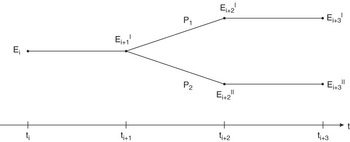
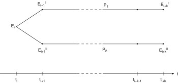
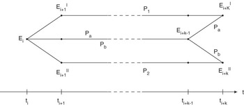
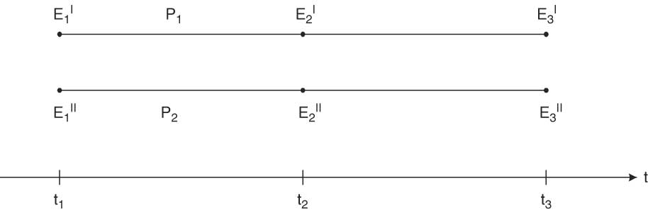
Working with the contingency framework it is natural to ask the following question: how closely are two states of the alternative set Ξi +k at any time ti +k ‘historically’ related with each other, i.e. with respect to an arbitrary previous state Ei from Ξi? For instance, the states Ei, Ei +k I and Ei +k II may be elements of the contingency graph Γ in Figure 13 and of the graph Γ′ in Figure 14.
The Contingency Proximity Degree (CPD) of Ei +k I and Ei +k II with respect to Ei = (1·1)/(k·k) = 1/k 2 (= minimal value).

CPD of Ei +k I and Ei +k II with respect to Ei = (1·1)/(1·1) = 1 (= maximal value).

Obviously, Ei +k I and Ei +k II have a ‘longer common history’ with respect to their common origin Ei in the example of Figure 14 than in the example of Figure 13. Thus, intuitively a ‘contingency proximity degree’ should give them different values in the two cases. Looking more closely at these two examples it becomes evident that Figures 13 and 14 in fact depict extreme cases of the possible proximity relation between Ei +k I and Ei +k II with respect to Ei *, as long as there exist paths connecting Ei with Ei +k I and with Ei +k II respectively (in the examples P 1, P 2, Pa, Pb): the proximity relation is maximal in Figure 14 and minimal in Figure 13.
Definition: The Contingency Proximity Degree (CPD) measures, in a contingency graph Γ, the contingency neighbourhood, or relatedness, of any two states Ei +k I and Ei +k II from the alternative set Ξi +k at time i + k (k > 0) with respect to an arbitrary previous event Ei in Γ at time i in the following way.
Let ΠI be the non-empty set of processes P 1I, …, Pm I connecting Ei with Ei +k I and ΠII the non-empty set of processes P 1II, …, Pn II connecting Ei with Ei +k II in Γ (k > 0). Then the Contingency Proximity Degree (CPD) is defined by
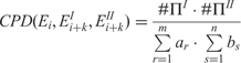
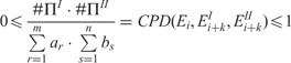
where ar = min{j | 0 ⩽ j ⩽ k, exists Pw II ∈ ΠII and exists Ei +k −j ∈ Pr I so that also Ei +k −j ∈ Pw II} for all r = 1, …, m = ΠI, and bs = min{h| 0 ⩽ h ⩽ k, exists Pz I ∈ ΠI and exists Ei +k −h ∈ Ps II so that also Ei +k −h ∈ Pz I } for all s = 1, …, n = ΠII under the further assumption that at least one ar and one bs are non-zero. Due to this definition
Let us comment on this definition.
1. The maximal value of CPD is
 (normalization by dividing by m· n)
2. The minimal value of CPD is
 (normalization by dividing by m· n)

Let us now consider three examples to give the reader an intuitive understanding of this definition.
(1) The CPDs in the two examples of Figure 13 and 14 above show the expected values.
(2) In Figure 15 the CPD of Ei +k I and Ei +k II with respect to Ei should be between the two extreme CPD values of Figures 13 and 14. In fact, 1/k 2 < 4/(1 + k)2 < 1 for k ⩾ 2.
Figure 15CPD of Ei +k I and Ei +k II with respect to Ei = (2· 2)/((k + 1)· (1 + k)) = 4/(1 + k)2.
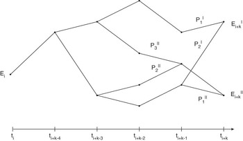
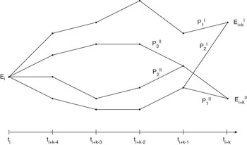
(3) Our third example is a little bit more complex. However, intuitively one would expect that the CPD of Ei +k I and Ei +k II with respect to Ei should be larger in Figure 16 than in Figure 17. In fact, the exact CPD values say that this intuition is right: 1/11<3/16.
Figure 16k = 5. CPD of Ei +k I and Ei +k II with respect to Ei = (2 · 3)/[(3 + 1)·(1 + 4 + 3)] = 6/32 = 3/16.
Figure 17k = 5. CRD of Ei +k I and Ei +k II with respect to Ei = (2·3)/[(5 + 1)· (1 + 5 + 5)] = 6/66 = 1/11.


Marco Lehmann-Waffenschmidt teaches applied and behavioural microeconomics at the University of Dresden. He studied mathematics and economics at the University of Heidelberg and the ETH Zürich. At the University of Karlsruhe (1983–1993) he obtained his diploma in mathematics, was an assistant professor, and received his doctorate and habilitation in economics. After holding research positions at the universities of Bonn and St. Gallen, and at the Artificial Intelligence Research Institute in Ulm, he was appointed as professor for Managerial Economics at the Department of Economics of the Technical University of Dresden. During the German reunification process Lehmann-Waffenschmidt served as a member of advisory boards of the government and parliament of the State of Saxony (recently in the ‘Sächsische Diätenkommission’ for developing a new law on remunerations of the members of the Saxonian parliament). His main research fields are mathematical economics, evolutionary economics, economics of sustainable development, and behavioural and experimental economics. He is actively engaged in the establishment of evolutionary economics in the teaching canon of economics and is the scientific organizer of an international workshop series for young economists in evolutionary economics (‘International Buchenbach Workshop for Young Evolutionary Economists’).