1. Introduction
Jet in crossflow (JICF) configurations are encountered frequently in engineering applications, for example the mixing of fuel and air in gas turbines for efficient combustion and reducing pollutant emission (Lefebvre Reference Lefebvre1998), film-cooling jets to cool turbine blades (Renze, Schröder & Meinke Reference Renze, Schröder and Meinke2008), aeroacoustic noise reduction (Zhao et al. Reference Zhao, Alimohammadi, Okolo, Kennedy and Bennett2018), and control of shock-induced flow separation (Wallis Reference Wallis1956), among others. The focus of this study is to gain a better understanding of the flow field generated by a row of spanwise-inclined jets injected into a supersonic boundary layer, as used for the control of shock-induced separation.
JICF topologies comprise several distinct vortical structures from different origins within the flow field, followed by complex interactions in between these structures and with the boundary layer. Because of the frequent occurrence of JICF configurations and the complexity of the flow, the JICF problem has been studied extensively. For studies of single jets in subsonic crossflow, see e.g. Kamotani & Greber (Reference Kamotani and Greber1972), Fric & Roshko (Reference Fric and Roshko1994) and Karagozian (Reference Karagozian2014), and for single jets in supersonic crossflow see e.g. Billig & Schetz (Reference Billig and Schetz1966), Gruber, Nejad & Dutton (Reference Gruber, Nejad and Dutton1995), Viti, Neel & Schetz (Reference Viti, Neel and Schetz2009), Génin & Menon (Reference Génin and Menon2010), Kawai & Lele (Reference Kawai and Lele2010), Rana, Thornber & Drikakis (Reference Rana, Thornber and Drikakis2011) and Sun & Hu (Reference Sun and Hu2018). A comprehensive summary of jet injection into crossflow is given by Mahesh (Reference Mahesh2013). Mostly, jets injected normal to the surface are investigated. Single jets injected at a spanwise or streamwise inclination have been studied by e.g. Fuller et al. (Reference Fuller, Mays, Thomas and Schetz1991a), Fuller, Thomas & Schetz (Reference Fuller, Thomas and Schetz1991b), Aso et al. (Reference Aso, Inoue, Yamaguchi and Tani2009), Sharma, Eswaran & Chakraborty (Reference Sharma, Eswaran and Chakraborty2020) and Sebastian, Lürkens & Schreyer (Reference Sebastian, Lürkens and Schreyer2020).
We are particularly interested in applying jets to control shock-induced separation in aerospace transportation and propulsion systems. In these applications, small air-jets are injected into the boundary layer upstream of the separation region, where they induce longitudinal vortices that increase turbulent mixing, thus transferring high-momentum fluid into the near-wall region. This makes the boundary layer less susceptible to separation and thus considerably reduces separation lengths and consequently also the detrimental effects of separation (Wallis Reference Wallis1956; Johnston & Nishi Reference Johnston and Nishi1990; Souverein & Debiève Reference Souverein and Debiève2010). Compared to the more common mechanical (micro) vortex generators, which also reduce separation effectively, jets injected as vortex generators (a) reduce the parasitic drag, (b) can be switched on and off as required, and (c) can be tuned to operate under different flow conditions. For separation-control purposes in two-dimensional (2-D) shock wave/boundary layer interactions (SWBLIs), jets inclined in the spanwise direction were observed to yield more favourable results than wall-normal jets or jets with a streamwise component (Wallis Reference Wallis1956; Johnston & Nishi Reference Johnston and Nishi1990). Wallis (Reference Wallis1956) found that the spanwise velocity component introduced by the spanwise inclination of the jets has the most relevant effect on their overall performance.
Despite small differences in flow organization in the controlled shock-induced separation flow fields and in the control efficiency, both mechanical and air-jet vortex generators (AJVGs) introduce fairly similar vortex structures. The key to control efficiency thus seems to be related to details in the induced flow topologies.
In our previous work (Sebastian et al. Reference Sebastian, Lürkens and Schreyer2020), we therefore performed a detailed analysis of the flow topology and resulting flow field downstream of the injection of a single spanwise-inclined jet in supersonic crossflow (JISCF) using large-eddy simulation (LES). The flow topology and phenomena are distinctly asymmetrical and much more complex than for perpendicular injection. (See § 1.1 for a short summary.)
Separation-control set-ups require injecting multiple jets for increased efficiency. Several geometric and flow parameters have to be considered here, amongst them the effects of injection angle (Wallis Reference Wallis1956; Barberopoulos & Garry Reference Barberopoulos and Garry1998; Verma & Manisankar Reference Verma and Manisankar2019), jet-orifice diameter (Ali et al. Reference Ali, Alvi, Manisankar, Verma and Venkatakrishnan2011; Szwaba Reference Szwaba2013), jet spacing (Verma & Manisankar Reference Verma and Manisankar2019; Ramaswamy & Schreyer Reference Ramaswamy and Schreyer2022), and jet-injection pressure ratio (Ali et al. Reference Ali, Alvi, Kumar, Manisankar, Verma and Venkatakrishnan2013; Ramaswamy, Hinke & Schreyer Reference Ramaswamy, Hinke and Schreyer2020). Note that Ali et al. (Reference Ali, Alvi, Kumar, Manisankar, Verma and Venkatakrishnan2013) investigate jets injected normal to the surface; all other references study inclined jets.
In such set-ups, the jets may be spaced at intermediate distances small enough that the flow features introduced by the individual jets interact, leading to an even more complex interaction flow field. Interactions between the jet-induced structures modify the boundary layer downstream of the injection location, which affects the separation-control effectiveness. A certain degree of interaction even appears to be beneficial for the control effect (see for example Verma & Manisankar Reference Verma and Manisankar2019; Ramaswamy et al. Reference Ramaswamy, Hinke and Schreyer2020).
These studies analyse mainly the overall effects of different AJVG parameters on the flow-control efficiency. Detailed information on the area in the vicinity of the injection location, the interaction among the jets and the flow topology – which are aspects key to the understanding of the flow field and the targeted improvement of control set-up designs – is mostly lacking. Only Ali & Alvi (Reference Ali and Alvi2015) discuss the flow topology in the vicinity of injection and the jet/jet interactions, but for jets injected perpendicular to the model surface.
However, their work does not provide details of the flow in the injection pipe and the direct vicinity of the injection region, and therefore of the formation of the induced structures. This information is required to understand the governing flow dynamics, though. Also, while the flow topology is similar, inclined injection induces an asymmetric counter-rotating vortex pair (CVP) of uneven strength and size (Sebastian et al. Reference Sebastian, Lürkens and Schreyer2020), whereas perpendicular injection induces symmetrical vortices. This difference becomes particularly influential when rows of multiple jets are injected, because it leads to very different jet/jet interactions. These interactions strongly affect the separation-control effectiveness when using rows of such jets to control shock-induced separation (Ramaswamy & Schreyer Reference Ramaswamy and Schreyer2022).
The detailed analysis of these complex flows requires data of high resolution and quality. Mahesh (Reference Mahesh2013) pointed out that while the measurement data quality has increased recently, only very few such data sets exist for high-speed flows. Also, high-fidelity simulations of such flows became possible only recently due to the advancement of high-performance computations (HPCs). The present work aims to generate high-quality data to provide answers to questions such as the owing. (1) Which jet/jet interactions exist? (2) What are their effects on the flow downstream? (3) How do they affect the control efficiency?.
Recent studies (e.g. Funderburk & Narayanaswamy Reference Funderburk and Narayanaswamy2019; Pickles & Narayanaswamy Reference Pickles and Narayanaswamy2020) indicate that vortex-generator control that energizes the boundary layer is much less effective in three-dimensional (3-D) SWBLI. However, the few works investigating the control of 3-D separation considered either mechanical vortex generators or jets injected normal to the surface. These methods generate symmetric CVPs. When arranged in a row, adjacent symmetric CVPs cancel each other out. This results in a faster dissipation of vorticity, which affects control effects adversely (Ali & Alvi Reference Ali and Alvi2015). Spanwise-inclined AJVGs, however, form long-lived asymmetric major CVPs and may therefore be more useful in 3-D SWBLI. Understanding their behaviour in 2-D flows is a necessary prerequisite to approach the control of 3-D separation required for many applications. Since the effects of spanwise-inclined jets in supersonic and low-hypersonic crossflows are very similar, such jets are potentially efficient and flexible control devices (Sebastian & Schreyer Reference Sebastian and Schreyer2022).
Aiming at the development of efficient AJVG setups, we need to gain a better understanding of the flow physics and governing mechanisms in the complex and unsteady flow field around spanwise-inclined jets. Understanding the jet/jet interactions is key to later assess and understand influences on shock-induced separation, as well as differences between different types of vortex generators. We therefore study jet/jet interactions and their influence on the boundary layer in the configuration of a row of jets injected into a supersonic crossflow at  $M_\infty =2.5$ and
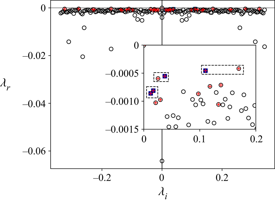
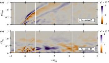
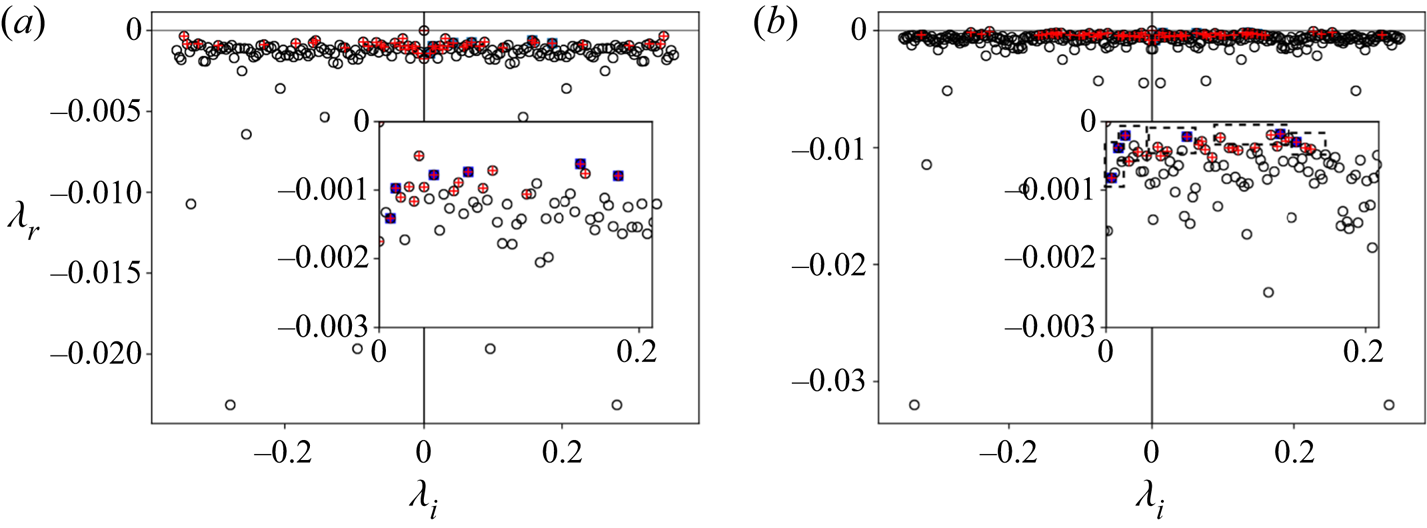
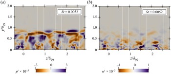
 $Re_\theta =7000$ by means of LES. The present work aims to investigate the influence of jet spacing on the jet/jet interactions and the resulting flow topology past injection. Additionally, flow visualizations were conducted at similar flow conditions to validate and compare the mean flow topology. The resulting database allows us to extract detailed information about the interactions among the jets, the jet-induced shock systems and the vortical structures, as well as the resulting modification of the downstream boundary layer. We also applied a 3-D dynamic mode decomposition to the flow field to study the dominant dynamic behaviour for different jet/jet interactions. Identifying the natural frequencies associated with the jet dynamics is also of interest in view of the choice of frequencies for active control approaches with jets that are triggered with periodic forcing functions (see e.g. Castelino & Gutmark Reference Castelino and Gutmark2021).
The numerical methods used to perform LES and the computational set-ups are described in § 2, experimental details are given in § 3, and our findings are discussed in § 4. In § 5, we summarize the key results and present concluding remarks. For better comprehensibility of our results and discussion, the flow field introduced by a single spanwise-inclined jet in supersonic crossflow, the flow topology in the vicinity of a row of jets injected perpendicular to the surface, and the effects of a row of spanwise-inclined AJVGs on shock-induced separation are summarized in §§ 1.1, 1.2 and 1.3, respectively.
1.1. Single spanwise-inclined jet in supersonic crossflow
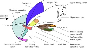
The flow topology for a single spanwise-inclined jet in supersonic crossflow is distinctly asymmetrical and more complex than for perpendicular injection (see Sebastian et al. (Reference Sebastian, Lürkens and Schreyer2020) and figure 1). The injected jet acts as an obstacle for the boundary layer, and a bow shock forms upstream. The boundary layer thickens and eventually separates, forming an oblique separation region upstream of injection. As the jet expands into the crossflow, it adjusts by forming a barrel shock that terminates in a Mach disk (see also Gruber et al. Reference Gruber, Nejad and Dutton1995). Upstream and downstream of the barrel shock, two secondary recirculation zones form. The crossflow on the side towards which the jet is injected is diverged laterally by the bow shock, wraps around the barrel shock, and then converges downstream with an offset in the jet-injection direction. The crossflow on the opposite side interacts strongly with the wake of the jet. As the diverged crossflow aligns in the streamwise direction, compression waves form and coalesce to an envelope shock (Morkovin, Pierce & Craven Reference Morkovin, Pierce and Craven1952).
Schematic illustration of spanwise-inclined jet/crossflow interaction. Adapted from Verma & Manisankar (Reference Verma and Manisankar2019).

A strongly asymmetric ensemble of vortices is induced (see figure 1). The most prominent feature is the major streamwise CVP. A secondary counter-clockwise rotating (CCR) upper-trailing vortex and a surface-trailing CVP are also induced. The upper-trailing vortex merges with the CCR vortex of the major CVP, contributing to the asymmetry of the major CVP. Close to the surface, an additional CCR surface-trailing vortex forms inside the herringbone-shaped downstream separation bubble. Farther downstream, this vortex merges with another CCR vortex (formed in the reattachment valley between the wings of the herringbone separation bubble) into the CCR surface-trailing vortex referred to as ‘type I’ in figure 1. Furthermore, a clockwise-rotating (CR) surface-trailing vortex (‘type II’) forms outside of the herringbone separation bubble. The CCR ‘type I’ vortex and the CR ‘type II’ vortex form an asymmetrical surface-trailing secondary CVP rotating in the direction opposite to that of the major CVP. As for the major CVP, the CCR vortex is stronger and subsists for a longer downstream distance. Far downstream of the injection ( $x>20d$, where
 $d$ is the jet diameter), only the major CVP persists and the associated momentum transfer makes the resulting flow field more resistant to separation (Sebastian et al. Reference Sebastian, Lürkens and Schreyer2020).
Upstream of injection, primary and secondary horseshoe vortices form due to the local recirculation zone. These vortices persist only in the close vicinity of the jet.
1.2. Flow topology in the vicinity of a row of jets injected normal to the surface
We summarize the flow around a row of perpendicularly injected jets in supersonic crossflow to provide a basis to discuss differences between normal and inclined injection.
The upstream influence is stronger for small ( $5d$) jet spacings, due to reduced entrainment of high-speed fluid between the jets and a stronger 2-D upstream shock. For moderate spacing (
 $10d$), the jet-induced oblique shocks merge and form a corrugated pattern. For further increased spacing, similar bow shocks as for single jets form. Also the wake downstream of the jets is stronger at larger jet spacing. The velocity is lowest along the jet centreline. For narrow spacings, the velocity deficits decrease with the wake region (Ali & Alvi Reference Ali and Alvi2015).
The spacing between the jets and the momentum coefficient strongly influence the generation and evolution of vorticity (Ali & Alvi Reference Ali and Alvi2015). For large and moderate spacings, the spatial extent of the symmetric CVP is of the order of the jet spacing. Coherent CVPs were observed until  $20d$ downstream of injection. Downstream, the CVPs lose their symmetry and strength. For moderate spacings, the CVPs are smaller and closer to each other. For small spacings, the CVPs interact more rapidly, the vortex pairs counteract, and the vorticity dissipates much faster. No discrete vortices exist beyond
 $5d$ downstream of injection. This behaviour is not ideal in view of separation-control applications.
No information is available on flow details in the injection pipe (which have a significant effect on the jet–crossflow interaction (Ramaswamy, Sebastian & Schreyer Reference Ramaswamy, Sebastian and Schreyer2021)) and close to the surface.
1.3. Influence of single-row AJVG arrays on shock-induced separation
The placement of spanwise-inclined jets in an array affects their separation-control effectiveness. The control efficiency is best for moderate injection pressure and jet spacing (Ramaswamy et al. Reference Ramaswamy, Hinke and Schreyer2020; Ramaswamy & Schreyer Reference Ramaswamy and Schreyer2022). It deteriorates for values below and above a certain range, which was attributed to varying degrees of interaction between the jet-induced structures. For large spanwise spacings of the jet orifices (approximately  $25d$–
 $32d$), the injected jets do not interact, and each jet induces a distinct upstream shock pattern (see Verma & Manisankar Reference Verma and Manisankar2019). When the jets are placed too closely together (e.g.
 $4d$), they form a merged bow shock spanning the entire row of jets (see Ramaswamy et al. Reference Ramaswamy, Hinke and Schreyer2020). For moderate spacings (
 $7d$–
 $13d$), the individual bow shocks overlap, resulting in a wrinkled shock pattern (see also our oil-flow visualizations in figure 5). Not only do the separation and reattachment locations, and thus the overall separation lengths, vary with jet spacing; the shape of the separation line is also affected. In the uncontrolled interaction, the separation line is straight and approximately 2-D. For moderate jet spacings, the separation line is spanwise corrugated, with local maxima in separation length downstream of the jet orifices.
It is still unclear which interaction processes account for the improved control effectiveness, as well as its deterioration for both increased and decreased jet spacing. Identifying and explaining these mechanisms are therefore the main objectives of our study.
2. Numerical methods
We performed LES of a row of jets injected into a supersonic turbulent boundary layer using the in-house multi-physics solver m-AIA (formerly referred to as the Zonal Flow Solver; Lintermann, Meinke & Schröder Reference Lintermann, Meinke and Schröder2020). The unsteady compressible Navier–Stokes equations are solved using a finite-volume method on a block-structured mesh. The convective fluxes are discretized using a second-order-accurate advection upstream splitting method (AUSM) by Liou & Steffen (Reference Liou and Steffen1993), and the viscous fluxes are discretized with a modified cell-vertex scheme at second-order accuracy (see Meinke et al. Reference Meinke, Schröder, Krause and Rister2002). The monotone upstream scheme for conservation laws (MUSCL) with the Venkatakrishnan limiter (Venkatakrishnan Reference Venkatakrishnan1995) is used to reconstruct the cell surface values and prevent steep and strong shocks from creating non-physical oscillations. The time integration is performed with a second-order-accurate five-stage Runge–Kutta scheme. The LES were performed using the monotonically integrated LES (MILES) approach (Boris et al. Reference Boris, Grinstein, Oran and Kolbe1992) to provide an efficient implicit LES framework, where the dissipation at high wavenumbers of the turbulence spectrum is mimicked by the numerical dissipation of the AUSM. The effects of the subgrid-scale model and order of the method on the overall accuracy of the solution have been discussed by Meinke et al. (Reference Meinke, Schröder, Krause and Rister2002). The numerical method has been validated thoroughly and proven suitable for the present case by computing turbulent boundary layers (El-Askary, Schroeder & Meinke Reference El-Askary, Schroeder and Meinke2003), shock wave/boundary layer interactions (Roidl Reference Roidl2012), and a JISCF problem (Sebastian et al. Reference Sebastian, Lürkens and Schreyer2020).
Unless specified otherwise, the following non-dimensionalization is used for the velocity  $\boldsymbol {u}=\tilde {\boldsymbol {u}}/\tilde {a}_0$, where the speed of sound is
 $\tilde {a}_0=\sqrt {\gamma \tilde {p}_0/\tilde {\rho }_0}$. Here,
 $\tilde {\cdot }$ denotes a dimensional quantity, and
 $\gamma$ is the ratio of specific heats. The subscript
 $0$ indicates values at stagnation conditions. The temperature, density and pressure are non-dimensionalized as
 $T=\tilde {T}/\tilde {T}_0$,
 $\rho =\tilde {\rho }/\tilde {\rho }_0$ and
 $p=\tilde {p}/\tilde {\rho }_0\tilde {a}^{2}_0$, respectively, and the viscosity is expressed using Sutherland's law. The lengths and distances are non-dimensionalized using the momentum thickness
 $\theta$, such that
 $\boldsymbol {x}=\tilde {\boldsymbol {x}}/\tilde {\theta }$. Time-averaged quantities and fluctuations are denoted with
 $\langle \,\cdot\, \rangle$ and superscript
 $'$, respectively. Time- and spanwise-averaged quantities are denoted with
 $\bar {\cdot }$. Furthermore, we use the following subscripts:
 $\infty$,
 $\delta _{99}$,
 $w$ for values in the freestream, at the edge of the boundary layer, and at the flat-plate surface (wall), respectively;
 $\theta$,
 $\tau$,
 $d$ for quantities based on the momentum thickness, wall shear stress, and injection pipe diameter, respectively; and
 $x$,
 $y$,
 $z$ for streamwise, wall-normal and spanwise quantities, respectively. The following superscripts are used:
 $+$ for values scaled in viscous units; ‘vd’ for van Driest scaled quantities; ‘jet’ for values at the jet exit; and ‘cf’ and ‘pl’ for quantities related to the crossflow and plenum subdomains, respectively.
2.1. Computational setup
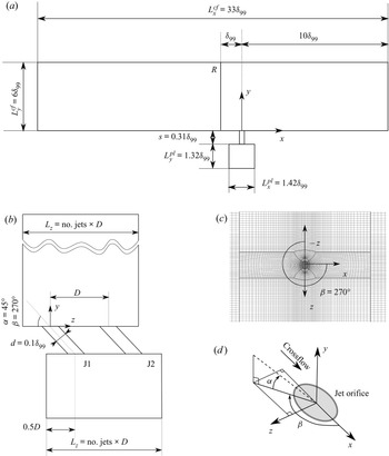
We study the configuration of a row of spanwise-inclined jets injected into a supersonic turbulent boundary layer on a flat plate. The computational domain (see figure 2) consists of three main regions: (a) the plenum supplying the air needed for injection, (b) the pipes used for injecting jets, and (c) the crossflow over the flat plate into which the jets are injected. The crossflow is characterized by a freestream Mach number  $M_{\infty }=2.5$ and a momentum-thickness Reynolds number
 $Re_{\theta }=\tilde {\rho }_\infty \tilde {u}_\infty \tilde {\theta }/\tilde {\mu }_\infty ={7000}$, based on the momentum thickness
 $\theta$ at the reference location
 $R$ (located one boundary-layer thickness
 $\delta _{99}$ upstream of the injection location), freestream velocity
 $u_\infty$, density
 $\rho _\infty$, and viscosity
 $\mu _\infty$. The geometry and dimensions of the computational domain match the experimental set-up of Ramaswamy & Schreyer (Reference Ramaswamy and Schreyer2021). Global flow parameters are given in table 1.
Schematic of the flow configuration and block-structured mesh. (a) Side view; (b) front view with two jet-injection pipes J1 and J2; (a,b) are not to scale.). (c) Top view of a zoom on the mesh in the vicinity of a jet (every fifth node is shown). The spanwise extent of the crossflow and plenum subdomains depends on the number and spacing  $D$ of the jets. (c) Definition of jet-injection angles.

Global flow parameters.

Four different jet spacings  $D$ were studied, with
 $D=4d, 8d, 16d, 32d$, where
 $d=0.1\delta _{99}$ is the injection pipe diameter. The extent of the crossflow domain in the streamwise, wall-normal and spanwise directions is denoted by
 $L_x^{cf}$,
 $L_y^{cf}$ and
 $L_z^{cf}$, respectively, and the dimensions of the plenum are
 $L_x^{pl}$,
 $L_y^{pl}$ and
 $L_z^{pl}$. For all cases, the length and height of the crossflow (or flat-plate) subdomain are
 $L_x^{cf}\times L_y^{cf}=33\delta _{99}\times 6\delta _{99}$ (see figure 2a). The spanwise extent of the crossflow and plenum subdomains was adapted to the jet spacing, such that
 $L_z=L_z^{cf} = L_z^{pl} =\text {no.\ jets}\times D$ (see figure 2b). The plenum has the streamwise and wall-normal dimensions
 $L_x^{pl}\times L_y^{pl}=1.42\delta _{99}\times 1.32\delta _{99}$; it is located at a distance
 $s=0.31\delta _{99}$ beneath the flat-plate surface. Geometric parameters for the different cases (D32, D16, D8 and D4 for set-ups with jet spacings
 $32d$,
 $16d$,
 $8d$ and
 $4d$, respectively) are given in table 2. The jets are fed with compressed air originating from the stagnation conditions in the plenum.
Geometric parameters for the cases studied.

The jet-injection pipes have circular cross-sections and are spanwise-inclined (or pitched) at angle  $\alpha =45^\circ$ (in the
 $y$–
 $z$ plane), and skewed at angle
 $\beta =270^\circ$ (in the
 $x$–
 $z$ plane) to the streamwise direction. The origin of the coordinate system is located at the exit of the first injection pipe on the flat-plate surface (see figures 2b,c). Subsequent jets are placed side by side in the
 $+z$ direction. Due to the
 $45^\circ$ spanwise inclination, both ends of the pipes (on the flat-plate surface and top surface of the plenum) have elliptical cross-sections. The major axis of the elliptical cross-section of the pipe exit on the flat-plate surface aligns with the
 $z$-axis, and the minor axis aligns with the
 $x$-axis (see figure 2c). The Reynolds number of the pipe flow is
 $Re_d=\tilde {\rho }_\infty \tilde {u}_\infty \tilde {d} / \tilde {\mu }_\infty =10^4$.
To capture accurately the influence of jet spacing on the interaction among multiple jets in a row and on the boundary layer, a DNS-like resolution is used near the flat plate. The mesh is gradually relaxed in the wall-normal direction. The mesh resolution in the crossflow region guarantees that  $\Delta x^+ \leq 10$,
 $\Delta y^+_{w}=1$,
 $\Delta y^+_{\delta _{99}}=12$ and
 $\Delta z^+\leq 5$. About 250 points in the wall-normal direction are used to discretize the boundary layer. A finer grid resolution is used in all directions in the vicinity of the injection location (see figure 2c). The first mesh point from the pipe surface in the radial direction is located at
 $\Delta r^+_{w}=1$. A mesh resolution similar to the one in the crossflow subdomain was used to discretize the plenum in the streamwise and spanwise directions. In the wall-normal direction, the first point from the top surface of the plenum is at
 $\Delta y^+=1$, and the mesh is gradually coarsened in the
 $-y$ direction. These mesh resolutions agree with previous studies by Kawai & Lele (Reference Kawai and Lele2010), Sun & Hu (Reference Sun and Hu2018) and Sebastian et al. (Reference Sebastian, Lürkens and Schreyer2020). Mesh points are clustered at both ends of the injection pipe to ensure a smooth transition between different regions of the domain and to capture the flow physics with great detail. Simulations were performed on the Cray XC40 HPC facility at HLRS, Stuttgart, Germany; on average, 5–8 million core hours were used per case.
The adiabatic no-slip wall boundary condition was imposed on the flat-plate surface, pipe surface, and top and side faces of the plenum. Periodicity was imposed in the spanwise direction of the crossflow subdomain. The geometric modelling combined with a periodic boundary condition in the spanwise direction is equivalent to injecting an infinite number of jets in a row. We imposed an outflow boundary condition on the top surface and outflow plane of the crossflow region, where values from within the domain were extrapolated.
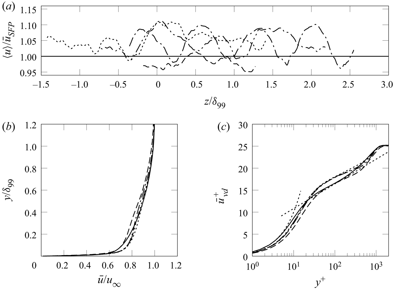
The crossflow subdomain was initialized with the mean flow field computed from a Reynolds-averaged Navier–Stokes (RANS) simulation of a turbulent flat-plate boundary layer under the crossflow conditions, which is used by the synthetic turbulence generator to feed the crossflow with realistic turbulence through the inflow plane (see Roidl Reference Roidl2012). The pipe and plenum were initialized with a zero velocity field and the freestream pressure and density. The jets were injected into the crossflow by prescribing the desired pressure at the bottom face of the plenum, which serves as the driving source of the jets. The plenum injection pressure was ramped up linearly from freestream to stagnation pressure. In addition, we performed a simulation of a supersonic turbulent boundary layer on a flat plate at the same Mach and Reynolds numbers with the dimensions of the crossflow subdomain for comparison and validation purposes (case SFP).
The injection of the array of jets is expressed using the momentum coefficient  $C_\mu$:
 \begin{equation} C_\mu=\frac{nb_{jets}(\gamma p A M^2)_{jet}}{(0.5\gamma p M^2)_\infty\times (\delta_{99}L_z)}, \end{equation}
where  $nb_{jets}$,
 $A_{jet}$,
 $M_{jet}$ are the number of jets, jet cross-sectional area, and jet Mach number close to the exit on the flat-plate surface, respectively. Here,
 $C_\mu$ gives the ratio of injected momentum (through the jets) to the crossflow, and also accounts for the geometrical parameters of each case. In the present paper, we study variations of
 $C_\mu$ over one order of magnitude (see table 2);
 $C_\mu$ increases from 0.00792 to 0.06336 when the jet spacing is reduced from
 $D=32d$ to
 $D=4d$ because of the higher momentum influx per unit span at smaller spacings.
3. Experimental configuration
Experimental investigations of similar configurations of jet injection in supersonic crossflow were conducted in the trisonic wind tunnel at the Institute of Aerodynamics, RWTH Aachen University, with the purpose of controlling a shock-induced separation. The facility is an intermittent vacuum storage tunnel and provides 2–4 s of stable flow. The test section has cross-section  $0.4\ {\rm m} \times 0.4\ {\rm m}$; optical access is provided by circular quartz windows on both side walls and on the top wall of the test section. The stagnation pressure and temperature of the freestream are equal to the ambient conditions in the laboratory. The selected Mach number of Mach 2.52 thus determines the freestream unit Reynolds number (
 $9.6 \times 10^6$ m
 $^{-1}$). The experimental conditions are closely matching the numerical simulation conditions; the Reynolds number based on the momentum thickness
 $\theta$ at a location
 $0.5\delta _{99}$ upstream of the jet orifices is
 $Re_{\theta }=7920$. The experimental parameters are summarized in table 3.
Experimental conditions.

Experimentally, the effect of jet spacing in spanwise-inclined jet injection with  $D=32d, 16d, 8d, 4d$ was studied on a
 $24^\circ$ compression–ramp model installed on a flat plate with total length
 $902$ mm. The model spanned the entire width of the test section (see Ramaswamy et al. (Reference Ramaswamy, Hinke and Schreyer2020) for more detailed information on the experimental set-up). Interchangeable AJVG inserts with one row of air-jet orifices are installed in the flat-plate model at
 $61.7\delta$ downstream of the leading edge (
 $7.69\delta _{99}$ upstream of the ramp corner). As in the matching numerical configuration, the jets are injected at a pitch angle
 $\alpha = 45^\circ$ with respect to the flat-plate surface, and skewed at an angle
 $\beta = 270^\circ$ with respect to the freestream, thus resulting in a purely spanwise injection. The AJVGs are supplied from a pressure plenum within the flat-plate model. The pressure and temperature in the plenum are monitored using a WIKA S-20 pressure transducer and a J-type thermocouple, respectively.
The global flow organization was assessed with an in-house-developed focusing- schlieren set-up (see Schauerte & Schreyer Reference Schauerte and Schreyer2018) with the focus plane along the model centreline. A Photron Fastcam SA5 CMOS camera recorded sequences of schlieren images at  $20$ kHz at resolution
 $704 \times 520$ pixel. The surface-flow features were studied on the basis of oil-flow visualizations, for which a mixture of Shell Tellus type 22 oil, TiO
 $_{2}$ particles, and a trace amount of oleic acid was used. We recorded the transient oil-flow pattern during the stable facility run time, using an RX100 digital camera with resolution approximately 0.18 mm px
 $^{-1}$ at 24 f.p.s. Thus the breakdown of the flow does not influence the interpretation of important flow features. Instantaneous images are used for the analysis. Quantitative values are obtained after averaging during the stable wind-tunnel operation over multiple runs; their standard deviations are as small as
 $0.1\delta _{99}$ with a confidence interval of 95 %.
4. Results
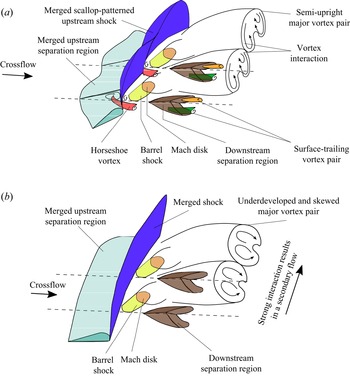
We will first discuss briefly the incoming boundary layer (§ 4.1) and the effect of jet spacing on the flow in the plenum and jet-injection pipes (§ 4.2). A detailed discussion of the effects of jet spacing on the mean and turbulent flow topology (§ 4.3), the coherent structures and their interaction and downstream evolution (§ 4.4), and the boundary-layer statistics in the near and far fields (§§ 4.5, 4.5.3, respectively) follow, completed by a conditional analysis and a discussion of the dynamic behaviour of the flow based on a 3-D dynamic mode decomposition (§ 4.6). Finally, a conceptual model of the flow field around air-jet arrays in supersonic crossflow is given (§ 4.7).
4.1. Incoming boundary layer
The crossflow represents a fully developed supersonic turbulent boundary layer with freestream Mach number  $M_\infty =2.5$, momentum thickness Reynolds number
 $Re_\theta ={7000}$, and friction Reynolds number
 $Re_\tau =\tilde {\rho }_w\tilde {\delta }_{99}\tilde {u}_\tau /\tilde {\mu }_w= 1093$ at the reference station
 $R$ without jet injection (where
 $\tilde {u}_\tau =\sqrt {\tilde {\tau }_w/\tilde {\rho }_w}$ is the friction velocity, and
 $\tilde {\tau }=\tilde {\mu }\,\partial \tilde {u}/\partial \tilde {y}$ is the shear stress). The corresponding van Driest scaled Reynolds number is
 $Re_\theta ^{vd}=\tilde {\rho }_w \tilde {u}_\infty ^{vd} \tilde {\theta }^{vd}/\tilde {\mu }_{w} = 2232$. We validated the boundary-layer profiles against the experiment of Ramaswamy & Schreyer (Reference Ramaswamy and Schreyer2021) at similar conditions (see also § 3) and the reference DNS data of an incompressible turbulent boundary layer at
 $Re_\theta =2500$ by Schlatter & Örlü (Reference Schlatter and Örlü2010) (see Sebastian et al. (Reference Sebastian, Lürkens and Schreyer2020) for more details).
4.2. Flow field in the plenum and jet-injection pipes
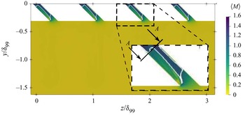
We will discuss the influence of jet spacing on the flow in the plenum and the jet-injection pipes on the basis of the local Mach number distribution in the spanwise/wall-normal plane at  $x=0$, shown in figure 3. The fluid entering the plenum is at stagnation conditions, and the fluid in the plenum is mostly at rest and thus not affected significantly by the jet spacing.
Mach-number contour and  $\langle M\rangle =1$ isoline (white solid line) in the plenum and jet-injection pipe (spanwise/wall-normal plane at
 $x=0$ for case D8).

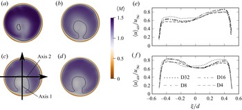
The flow accelerates strongly inside the jet-injection pipe, and attains sonic speed in the vicinity of the plenum–pipe intersection (see figure 3, zoomed detail). Due to the spanwise inclination  $\alpha =45^\circ$, the flow separates locally inside the jet-injection pipe (visible as the subsonic region close to the plenum–pipe intersection). The flow in the jet-injection pipe is 3-D and complex (see Sebastian et al. Reference Sebastian, Lürkens and Schreyer2020), and the flow at the pipe exit on the flat-plate surface is supersonic with
 $\langle M\rangle = 1.4\unicode{x2013}1.5$ (see figures 4a–d). The Mach number distributions for different spacings differ slightly just before injection. However, the overall shape of the distribution is maintained, as visible in the mean axial velocity profiles (see figure 4e). The profiles are shown along the axes marked in figure 4c;
 $\xi$ denotes distances on these local axes. The jet profile is symmetric along axis 2 for all cases, whereas along axis 1, a slight asymmetry is visible for
 $\xi /d<-0.2$. The asymmetry increases with decreasing jet spacing. Comparing cases
 $D=32d$ and
 $4d$, for instance, the small hump in the profile vanishes, and the mean axial velocity profile has a plateau for
 $\xi /d<-0.2$.
Mach number distributions in the injection pipe close to the jet exit (cross-section  $A$ marked in figure 3) superimposed with
 $\langle M\rangle =1$ contour (black solid line): (a) D32, (b) D16, (c) D8, (d) D4. (e,f) Axial jet profiles along (e) axis 1 and (f) axis 2.

4.3. Shock structures and flow topology
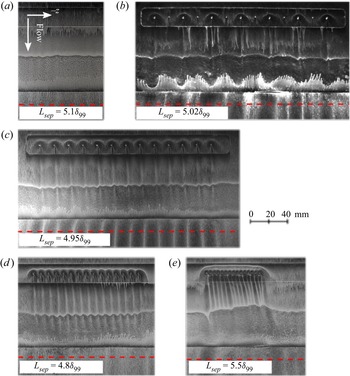
The injection of a spanwise-inclined jet into a supersonic crossflow induces the formation of a complex system of shocks and vortical structures (Sebastian et al. Reference Sebastian, Lürkens and Schreyer2020; see also § 1.1). The influence of jet spacing on this flow structure will be discussed on the basis of oil-flow visualizations of the  $24^\circ$ compression–ramp flow with and without AJVGs (figure 5) and mean density contours at
 $y=0.35\delta _{99}$ (figure 6) from LES. Due to the periodic boundary condition in the spanwise direction, the simulation reproduces the flow in the central region of the AJVG array that is least affected by the boundary and/or corner effects.
Oil-flow visualization of  $24^\circ$ compression–ramp flow: (a) uncontrolled case, with AJVG control with jet spacings; (b)
 $D=32d$ (every second orifice in the
 $D=16d$ inlet was sealed inside the plenum); (c)
 $D=16d$; (d)
 $D=8d$; (
 $e$)
 $D=4d$. Dashed lines represent flow reattachment.

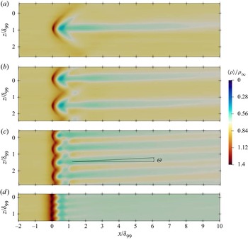
Time-averaged density in wall parallel plane at  $y=0.35\delta _{99}$: (a) D32, (b) D16, (c) D8, (d) D4. Angle
 $\varTheta$ denotes the deflection of the flow into the jet-injection direction.

The jet-induced shocks are visible as high-density regions in figure 6 and can be distinguished equally well in the oil-flow visualizations (figure 5). For the largest spacings (case D32), we observe individual fully formed bow shocks, as usually found for single jets injected into a supersonic crossflow. When the jet spacing is reduced to  $D=16d$, weak interactions between the individual bow shocks emerge (see figures 5c and 6b). For case D8, where the best separation-control effectiveness has been observed, the interactions among these shock structures increase and a scallop-shaped pattern forms in the spanwise direction (see figures 5d and 6c). Upon further reduction of the jet spacing to
 $D=4d$, the interactions among the upstream shock structures strengthen, and they merge into a single oblique shock located farther upstream than in all other cases (see figures 5e and 6d). The overall topology of the jet-induced upstream shock for spanwise-inclined injection at different jet spacings is very similar to normal injection at equivalent spacing (see Ali & Alvi Reference Ali and Alvi2015).
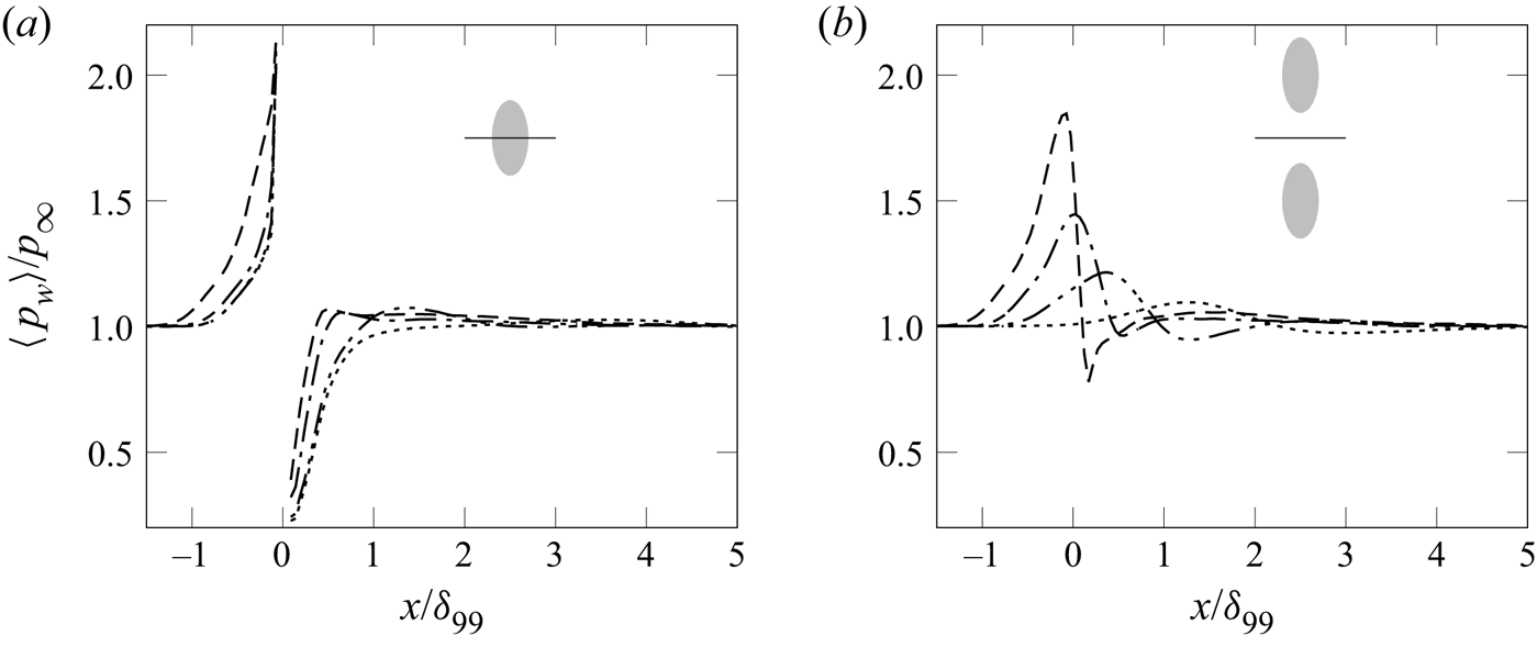
For a quantitative discussion of the influence of jet spacing on the shock structures in the vicinity of the injection location, we consider the conditional time-averaged wall pressure along the jet centreline and mid-plane between the jets (see figures 7a,b, respectively). The increase in wall pressure along the jet centreline upstream of injection is related to the jet-induced bow shock. For large jet spacings (D32 and D16), the pressure curves overlap in this region. The pressure is only slightly higher for case D8. For D4, the pressure starts to rise earlier (from  $x/\delta _{99}\approx -1.3$ instead of
 $x/\delta _{99}\approx -1.0$), confirming a larger standoff distance of the upstream shock and thus a larger local separation region. Downstream of injection, the wall-pressure level recovers with an expansion. For the smallest jet spacing (D4), the pressure recovers the fastest, and the streamwise recovery length – which indicates the size of the downstream separation zone – increases with jet spacing.
Conditional time-averaged wall-pressure distribution for: ( $\cdots$) D32, (–
 $\cdot \cdot$ –) D16, (–
 $\cdot$ –) D8, (– – –) D4, (a) along the jet centreline, and (b) between jets.

In the mid-plane between the jets, the wall-pressure intensity maximum is largest for the smallest spacing due to the increased interaction between the upstream shock structures. With increasing jet spacing, the magnitude of the maximum wall pressure and the interactions between the shocks decrease, and the intensity maximum moves downstream. For case D4, the maximum of  $\langle p_w\rangle =1.8p_\infty$ is located at
 $x/\delta _{99}=-0.05$; for D32, the maximum has decreased to
 $1.05p_{\infty }$ and moved downstream to
 $x/\delta _{99}=1.3$.
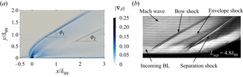
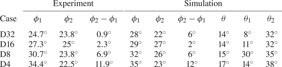
The shock angles were extracted from contours of the time-averaged mean-density gradient in the streamwise/wall-normal plane along the jet centreline and the corresponding schlieren image from the experiment (case D8 is shown as an example in figure 8). In addition to the bow and envelope shocks, the schlieren images also show the incoming boundary layer (BL), Mach waves forming at the edges of the AJVG insert, and the shock and flow separation of the compression–corner interaction downstream. The angles of the bow and envelope shocks to the streamwise  $x$-axis,
 $\phi _1$ and
 $\phi _2$, respectively, are given in table 4. With decreasing jet spacing (from
 $D=32d$ to
 $D=4d$), the upstream shock steepens (
 $28^\circ \leq \phi _1\leq 35^\circ$). Also, the envelope shock steepens initially (
 $22^\circ \leq \phi _2\leq 27^\circ$) and moves upstream (from
 $x=1\delta _{99}$ to
 $x=0.7\delta _{99}$) when the spacing is reduced from
 $D=32d$ to
 $D=16d$. Upon further reduction to
 $D=8d$, angle
 $\phi _2=26^\circ$ decreases again and the envelope shock shifts downstream (
 $x=1.3\delta _{99}$). For spacings below the region where effective separation control can be achieved (case D4), the envelope shock becomes less steep (
 $\phi _2=23^\circ$), and shifts farther upstream to the vicinity of the injection location (
 $x/\delta _{99}=0.2\unicode{x2013}0.3$). The envelope shock is at a flatter angle than the upstream shock for all jet spacings. Experiments and simulations yield similar trends, although the experimentally observed angles are slightly smaller (by
 $2^\circ \unicode{x2013}3^\circ$). Verma & Manisankar (Reference Verma and Manisankar2019) observed similar trends for the shock structures at Mach 2.
Visualization of shock structures in a streamwise/wall-normal plane for case D8: (a) magnitude of the time-averaged density gradient along the jet centreline from LES; and (b) schlieren image of controlled compression–ramp flow with AJVG. In (a),  $\phi _1$ and
 $\phi _2$ are the angles of the bow and envelope shocks with respect to the
 $x$-axis.

Characteristic angles of flow features induced by rows of jets in supersonic crossflow, where  $\phi _1$ and
 $\phi _2$ are the angles of the bow and envelope shocks to the
 $x$-axis, and
 $\theta$,
 $\theta _1$ and
 $\theta _2$ are the angles of the herringbone structure downstream of injection. See figures 8 and 9 for definitions.

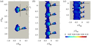
The 3-D shape and extent of the separation regions are visualized with the isosurface of  $\langle u\rangle =0$ in figure 9. For cases D32 (not shown) and D16, individual oblique separation regions with spanwise dimension
 $0.6\delta _{99}$ form upstream of each injection location due to the bow shock (
 $-0.5\leq x/\delta _{99} \leq -0.05$ and
 $-0.4\leq z/\delta _{99} \leq 0.2$). For jet spacing
 $D=0.8\delta _{99}$, these individual separation zones have merged into one large-scale separation with a spanwise-corrugated upstream edge. The differences in the onset of upstream separation between cases D32, D16 and D8 are minor. Upon further reduction of the spacing (case D4), the separation line is shifted farther upstream and the spanwise wave pattern is no longer observed (see figure 9c). These findings agree nicely with the oil-flow visualization results (see figure 5). The merged region of the separation zone is relatively flat and limited to the near-wall region: at
 $x=-0.25\delta _{99}$, recirculating flow is observed only below
 $y<0.1d$ for D4, and below
 $y<0.15d$ for D8. The height of the separation region increases with increasing jet spacing (see figure 9).
Isosurface of  $\langle u\rangle =0$ coloured with wall-normal distance: (a) D16, (b) D8, (c) D4. Angles
 $\theta$,
 $\theta _1$ and
 $\theta _2$ characterize the herringbone separation region.

The separation regions forming downstream of each jet-injection location are quasi-herringbone-shaped (see figure 9). Their size decreases with spanwise spacing, in particular for D4. The separation regions for D32 and D16 are very similar. This agreement indicates that both cases represent spacings for which the introduced structures do not yet interact to a significant extent. For case D8, the separation region is slightly wider (by  $0.15\delta _{99}$) and for the smallest spacing, case D4, the width decreases considerably (
 $0.08\delta _{99}$).
Also, the spanwise deflection angles of these downstream separation zones ( $\theta$,
 $\theta _1$ and
 $\theta _2$; see figure 9 and table 4) change with jet spacing: the overall deflection
 $\theta$ increases for small spacings (from
 $14^\circ$ to
 $17^\circ$), indicating a stronger influence of the spanwise velocity component. The inner angle
 $\theta _1$ of the inner separation wing (i.e. the wing closer to the streamwise
 $x$-axis) increases from
 $8^\circ$ to
 $30^\circ$, with reduced spacing from D32 to D8, and then decreases again. The outer angle
 $\theta _2$ of the outer wing increases to a smaller extent (from
 $32^\circ$ to
 $38^\circ$), but continues to do so also for spacings below
 $D=8d$. Due to the varying deflection from the
 $x$-axis, the location of minimum
 $\langle u\rangle$ is at different spanwise locations.
The downstream separation bubble has a larger wall-normal extent than the upstream separation bubble for all tested cases (see figure 9).
The jet injection induces vortical structures in the crossflow, whereof the major CVP is most prominent. The behaviour of these structures is discussed in detail in § 4.4; here, we will discuss only their effect on the flow topology.
The major CVP is recognizable in the low-density regions in the streamwise/spanwise distribution of  $\langle \rho \rangle$ at
 $y=0.35\delta _{99}$ (see figure 6). For D8 and D4, the interaction between adjacent jets manifests itself in a linear wave pattern at
 $x=\delta _{99}$, with highest and lowest peak amplitudes
 $\langle \rho (y=0.35\delta _{99})\rangle \approx 0.8\rho _\infty$ and
 $0.5\rho _\infty$, respectively, for D8, and
 $0.65\rho _\infty$ and
 $0.6\rho _\infty$ for D4. Farther downstream, at
 $x=3\delta _{99}$, the averaged densities do not change significantly, except for very narrow spacings (D4), where the wave pattern disappears.
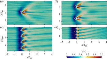
The jet-induced vortical structures are also visible as regions of higher Mach number ( $M\geq 1.0$) in figure 10. The structures merge more and more with decreasing jet spacing, indicating that the wakes of the jets interact increasingly strongly. While for the D32 and D16 cases no interaction is evident yet, a spanwise undulation in the Mach number pattern directly downstream of injection is observed for D8 (see figures 10a–c, respectively). Upon further reduction of the jet spacing, this pattern develops into a spanwise inclined saw-tooth pattern (see figure 10d). Also, the upstream bow shock is visible as a low-Mach-number region. The shock and downstream traces of the jet-induced low- and high-speed streaks agree nicely for the oil-flow visualizations (figure 5) and LES (figure 10).
Time-averaged Mach number distribution in a wall-parallel plane at  $y^+=15$ superimposed with the isoline of
 $\langle u\rangle =0$ for cases (a) D32, (b) D16, (c) D8, (d) D4.

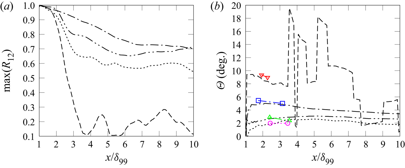
The spanwise deflection of the flow in the direction of injection visible in figures 6 and 10 is quantified by calculating the mean flow-deflection angle  $\varTheta$ using the lag of the maximum two-point spanwise cross-correlation coefficient of
 $\langle u\rangle$ (
 $R_{12}$) between reference location
 $x_1=\delta _{99}$ and all downstream locations, given in (4.1), and the distance between the two corresponding streamwise locations as given in (4.2):
 \begin{gather} R_{12}=\frac{\langle u\rangle_{x_1} \langle u\rangle_{x_2}} {{\rm std}(\langle u\rangle)_{x_1} \,{\rm std}(\langle u\rangle)_{x_2}}, \end{gather}
 \begin{gather}\varTheta=\tan^{{-}1}\left(\frac{\Delta z}{\Delta x}\right). \end{gather}
The downstream evolution of flow-deflection angle at  $y=0.1\delta _{99}$ is shown in figure 11(b). For cases D32 and D16, the average deflection angle is
 $2^\circ \leq \varTheta \leq 3^\circ$. For case D8, the deflection is slightly stronger (
 $\varTheta =5^\circ$) for
 $x<3\delta _{99}$. For all three cases, the deflection angle decreases in the downstream evolution. For D4, the mean flow deflection is stronger (
 $8^\circ \leq \varTheta \leq 9.5^\circ$) in the vicinity of injection (see also figure 11b). Due to weak correlations in the far field (
 $R_{12}<0.35$ for
 $x>3\delta _{99}$), the deflection-angle estimation in this region is not reliable. Angles computed from the oil-flow visualizations shown in figure 5 are given for comparison. In the experiment, deflection angles were calculated in between the locations of the AJVG insert and the respective separation line, with an uncertainty of about
 $1^\circ \unicode{x2013}2^\circ$. In general, the experimental and numerical results agree reasonably well. For the smallest jet spacing (
 $D=4d$), however, the angle computed from the experiment is slightly larger.
Streamwise evolution of (a) the maximum spanwise cross-correlation coefficient of  $\langle u\rangle$ between
 $x=\delta _{99}$ and the respective downstream locations at
 $y=0.1\delta _{99}$, and (b) the flow-deflection angle, for (
 $\cdots$) D32, (–
 $\cdot \cdot$ –) D16, (–
 $\cdot$ –) D8, and (– – –) D4. Coloured symbols denote deflection angles in the oil-flow visualizations in figure 5 (red for D4, blue for D8, green for D16, and magenta for D32).

The deflection angle increases with the jet/jet interactions, i.e. decreasing jet spacing. The jets affect the mean flow almost across the entire thickness of the boundary layer (not shown here). Towards the boundary-layer edge,  $\varTheta$ decreases and drops to zero. Only for D4, the deflection intermediately increases outside the viscous sublayer, then remains constant for
 $10\leq y^+ \leq 100$ (equivalent to
 $0.01\leq y/\delta _{99}\leq 0.1$) before it decreases.
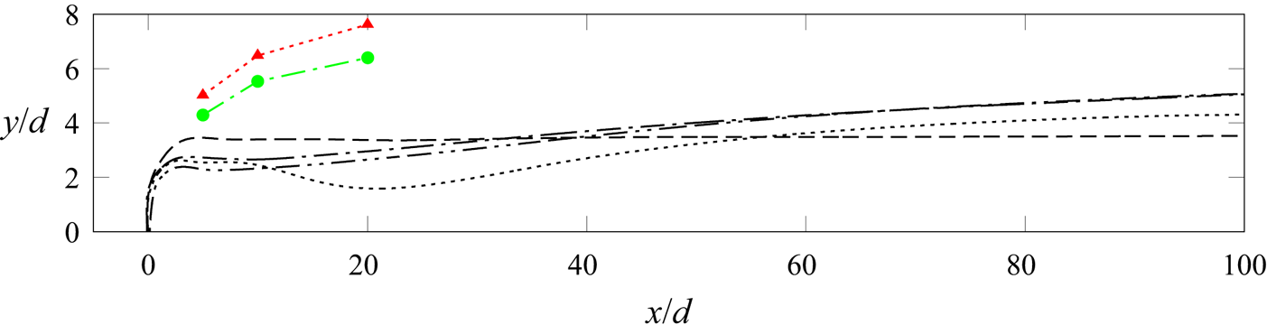
The penetration depth of the jets into the crossflow seems to be affected by the level of interaction between the jet-induced structures (see figure 12, showing the trajectory of the streamline passing through the jet centre). Directly downstream of injection, the penetration depth is about 40 % larger for case D4 ( $y=3.7d\equiv 0.37\delta _{99}$) than for all other cases due to the stronger blockage by the upstream shock. This level remains constant for a downstream distance of at least
 $100d$ (
 $\equiv 10\delta _{99}$). For all other cases, the penetration depth increases slowly (up to
 $y=5.2d\equiv 0.52\delta _{99}$ for D16 and D8) due to the vortex liftoff. Strong jet/jet interactions thus seem to impede vortex liftoff. For D32, the case without noticeable jet/jet interactions, the penetration depth decreases locally (at around
 $x=20d\equiv 2\delta _{99}$) before it increases to a level slightly below that reached for D16 and D8.
Jet penetration depth for cases ( $\cdots$) D32, (–
 $\cdot \cdot$ –) D16, (–
 $\cdot$ –) D8, (– – –) D4. Normal injection data from Ali & Alvi (Reference Ali and Alvi2015): red triangles and green circles are used for intermediate and large spaced arrays, respectively.

The observations for case D4 regarding the penetration depth and spanwise deflection of the flow suggest a secondary flow in the spanwise direction and an absence or early decay of the major CVP. These aspects will be discussed further in the following subsections.
The major effect of spanwise jet inclination is the formation of asymmetric CVPs of uneven strength and size. Jet/jet interactions are thus very different than for wall-normal injection (see also § 1.3). These interactions strongly affect the vortex development and their effect on the boundary layer. Jet/jet interactions do not affect the penetration properties for normal injection, and jet arrays with varying spacings achieve penetration similar to that for single jets (Ali & Alvi Reference Ali and Alvi2015; see figure 12). For spanwise-inclined injection, however, the penetration depth increases when the jet spacing is reduced from large (D32) to intermediate (D8) values. A comparison of the respective jet-penetration depths is shown in figure 12. Note that in the normal injection cases from Ali & Alvi (Reference Ali and Alvi2015), the momentum flux coefficients  $C_\mu$ and the momentum fluxes
 $J$ are larger than for the present case (see also table 4). The overall penetration is thus stronger for these normal injection cases.
4.4. Turbulent coherent structures and their interaction
For spanwise-inclined jet injection, the crossflow is diverged strongly in the direction of injection, and the crossflow on the side opposite to the injection direction interacts with the jet wake, forming an asymmetric ensemble of vortices (see figure 1, § 1.1, and Sebastian et al. Reference Sebastian, Lürkens and Schreyer2020). The most prominent structure is the major CVP, which redistributes the momentum across the boundary layer.
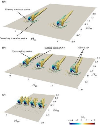
In this subsection, we will discuss the influence of jet spacing on the vortical structures induced by an array of jets and the interactions among them. A visualization of these structures, using isosurface plots of the constant  $Q$-criterion (
 $Q=0.05$) computed from the mean velocity field of LES, is shown in figure 13 for cases D16, D8 and D4. The characteristics of most induced vortex structures are similar for cases D8, D16 and D32 (D32 is not shown in figure 13 since it fully matches D16), in the sense that the CR major vortex is stronger than the CCR major vortex and persists for a longer downstream distance (up to
 $x=1.8\delta _{99}$ and
 $\delta _{99}$ downstream of the injection location, respectively). The horseshoe vortices upstream of the jet behave differently once the jet spacing is reduced to
 $D=8d$ and the upstream recirculation bubbles of neighbouring jets start to merge (see also figure 9): the spanwise extent of the vortices decreases, and the secondary horseshoe vortex becomes weaker. This trend continues with further decreased spacing (
 $D=4d$): the width of the primary horseshoe vortex decreases to approximately the injection pipe diameter
 $d$, and the secondary vortex vanishes completely.
Isosurface of the  $Q$-criterion (
 $Q=0.05$) computed from the mean velocity field and coloured with
 $\langle \omega \rangle _x$ for cases (a) D16, (b) D8, (c) D4.

The jet spacing strongly influences the major CVP. For  $D=4d$, the major CVP perishes much quicker (at
 $x=\delta _{99}$). The streamwise evolution of the maximum spanwise cross-correlation
 $R_{12}$ of
 $\langle u\rangle$, computed with (4.1), sheds further light on the downstream longevity of the introduced structures. The highest correlation values (
 $\max (R_{12})=0.7$ at
 $x=10\delta _{99}$) and slowest decrease in the downstream direction occur for D8 (see figure 11a). The high separation-control effectiveness observed for this case (see Ramaswamy & Schreyer Reference Ramaswamy and Schreyer2021, Reference Ramaswamy and Schreyer2022) thus seems to be related to the maintained coherence of the structures induced by the vortex generators. For all other cases, a strong initial drop in correlation occurs within a distance
 $3\delta _{99}\unicode{x2013}4\delta _{99}$ downstream of the jet injection. The most precipitous decrease (to
 $0.1$ at around
 $x=3.5\delta _{99}$) is observed for D4, for which the separation length even increases. Interestingly, a difference between the D16 and D32 cases is observed here: correlation values are higher by about 0.1 along the observed streamwise distance for D16, which indicates that weak interactions do already occur at this jet spacing.
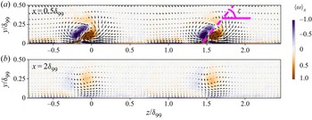
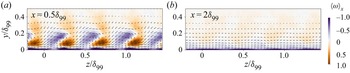
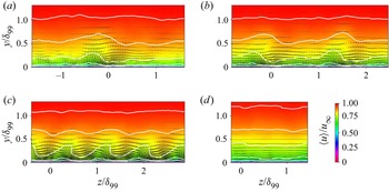
The behaviour and evolution of the major CVP are reflected in the distribution of the time-averaged streamwise vorticity in the spanwise/wall-normal plane. Its distribution at  $x=0.5\delta _{99}$ and
 $2\delta _{99}$, superimposed with the
 $\langle v\rangle -\langle w\rangle$ vectors, is shown in figures 14–16. The major CVP in cases D32 and D16 has the same behaviour and dimensions, thus we present the result only for case D16 (figure 14). For D32 and D16, the CVP is of uneven size since the CCR upper-trailing vortex merges with the CCR major vortex (see figure 14a). The resulting kidney-shaped CCR vortex lies above the circular CR major vortex. Strong downwash occurs on both sides of the major CVP (stronger on the side of the CR vortex), transporting fluid from the outer part of the boundary layer to the near-wall region. At
 $x=2\delta _{99}$ (see figure 14b), the strength of the major CVP has reduced and its diameter has increased (to a spanwise extent of approximately
 $0.6\delta _{99}\equiv 6d$). It lifts off the flat-plate surface, with the vortex core at
 $y\approx 0.25\delta _{99}$. The vorticity is concentrated at
 $-0.4\leq z/\delta _{99}\leq 0.2$. The weaker vortex dissipates faster, whereas the stronger vortex persists for a longer downstream distance and enlarges with gradual vorticity dissipation. At large spacings, such as D32 and D16, the adjacent CVPs do not interact and stay independent in the downstream evolution. Similar observations were also made by Pauley & Eaton (Reference Pauley and Eaton1988) with uneven vortex pairs in subsonic flow.
Time-averaged streamwise vorticity component  $\langle \omega \rangle _x$ superimposed with
 $\langle v\rangle -\langle w\rangle$ vectors in spanwise/wall-normal planes at (a)
 $x=0.5\delta _{99}$ and (b)
 $2\delta _{99}$ for case D16. Here,
 $\zeta$ denotes the angle between the major CVP structure and the flat-plate surface.

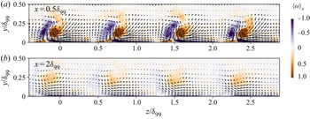
Time-averaged streamwise vorticity component  $\langle \omega \rangle _x$, superimposed with
 $\langle v\rangle -\langle w\rangle$ vectors, in spanwise/wall-normal planes for case D8.

Time-averaged streamwise vorticity component  $\langle \omega \rangle _x$, superimposed with
 $\langle v\rangle -\langle w\rangle$ vectors, in spanwise/wall-normal planes for case D4.

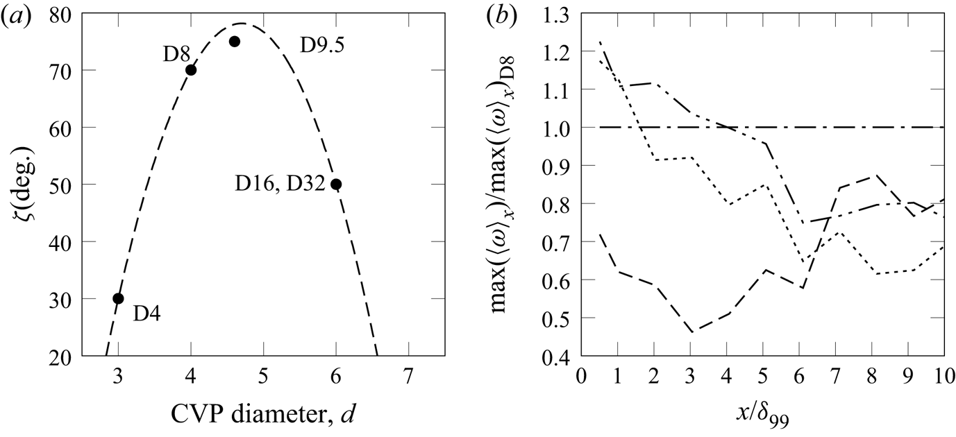
The maximum streamwise component of the mean vorticity, which traces the CR major vortex (see figure 17b), is strongest for case D8 in the far field – as was the cross-correlation  $R_{12}$ and thus the major CVP's longevity. For easier comparability between cases, the vorticity is normalized with the evolution for D8. In the direct vicinity of the jet (
 $x<4\delta _{99}$), the vorticity for D32 and D16 is up to 20 % larger. Farther downstream, however, the vorticity for these cases drops below the value for D8; at
 $x=10\delta _{99}$, only about 70 %–75 % is maintained.
(a) Characteristics of the CVP structure for different jet spacings:  $\zeta$ versus CVP diameter. Dashed line: polynomial fit through data points D32, D16, D8 and D4. (b) Streamwise evolution of ratio of maximum vorticity with respect to case D8 for cases (
 $\cdots$) D32, (–
 $\cdot \cdot$ –) D16, (–
 $\cdot$ –) D8, (– – –) D4.

The orientation of the CVP structure in the wall-normal/spanwise plane with respect to the flat-plate surface varies with jet spacing; it is quantified by means of the angle  $\zeta$ (see figure 14a). For cases D32 and D16, the CVP is oriented at angle
 $\zeta \approx 50^\circ$.
For D8, the individual CVPs are of smaller diameter ( $\Delta z\approx 0.4\delta _{99}(\equiv 4d)$ at
 $x=0.5\delta _{99}$; see figure 15) than for D32 and D16. The kidney-shaped CCR vortex still lies above the circular CR major vortex, but stands more upright (
 $\zeta \approx 70^\circ$). Interactions amongst neighbouring major CVPs cause the downwash induced by the respective CR vortices to draw in fluid from the CCR major vortex of the adjacent vortex pair, resulting in the more upright position of the CVP structure. This behaviour enhances the momentum transfer across the boundary layer (as will be shown in detail in § 4.5). As for D32 and D16, the vortex pair lifts off the flat-plate surface farther downstream (
 $x=2\delta _{99}$), moving the vortex core from
 $y=0.1\delta _{99}$ to
 $y=0.25\delta _{99}$, and the diameter of the major CVP increases to
 $\Delta z=0.6\delta _{99}(\equiv 6d)$. Following Mehta et al. (Reference Mehta, Shabaka, Shibl and Bradshaw1983), counter-rotating vortices can be classified as ‘common flow up’ and ‘common flow down’ based on the direction of the secondary flow between them, which can be directed either away from or towards the walls. When arranged in a row, the CVP core region corresponds to ‘common flow up’, and the region between adjacent CVPs to ‘common flow down’. Symmetric common-flow-down vortex pairs move apart as they convect downstream (Pauley & Eaton Reference Pauley and Eaton1988), which prevents interactions between such vortex pairs. However, in the present case, the asymmetry of the CVP modifies this behaviour: the stronger CR vortex draws in the weaker CCR vortex from the adjacent CVP, which leads to enhanced vorticity and stronger downwash.
Further decrease in jet spacing (case D4) hinders the development of full individual CVPs (see figure 16). Instead, the jets strongly interact with each other and a nonlinear spanwise wave pattern forms up to  $y\leq 0.2\delta _{99}$ with weakened and strongly spanwise-skewed CVPs (
 $\zeta \approx 30^\circ$), where the CCR vortex still mostly lies above the CR major vortex. The CVP now has an approximate spanwise width of only
 $0.3\delta _{99}$. At
 $x=2\delta _{99}$, these structures have almost completely vanished (see figures 13c and 16b), and a secondary flow along the direction of injection with a weak undulation pattern has formed. Compared to D8, the maximum vorticity for D4 is much lower from the beginning and drops further to 45 % at
 $x=3\delta _{99}$ (see figure 17b). Farther downstream, the secondary flow in the spanwise direction induces additional vorticity, but not enough to recover the value for D8 (see also § 4.3). The secondary flow and lack of fully developed CVPs reduce the control effectiveness of AJVGs with small jet spacing (see figure 5e). Note that in this oil-flow visualization for the control of a compression–ramp interaction with a
 $D=4d$ AJVG array (figure 5e), the separation zone upstream of the ramp corner is not symmetric and increases by about 11.3 % in the jet-injection direction. The reason for this behaviour is, besides corner effects, that the secondary spanwise flow component strengthens along the direction of jet injection, which results in earlier separation. In the LES, this effect is impeded by the imposed spanwise periodicity.
It appears that the diameter of the asymmetric CVP and its orientation in the wall-normal/spanwise plane are indicators of the degree of favourable interactions between neighbouring spanwise-inclined jets; these parameters therefore might contribute to indicating control effectiveness in AJVG control applications. The relation between  $\zeta$ and the diameter of the major CVP for the spacings investigated here is shown in figure 17(a). For jet spacings large enough to allow for the development of independent jet wakes, the CVP has the largest diameter (
 $0.6\delta _{99}$ for D32 and D16). Upon reduction of the spacing to a value that allows for interactions amongst adjacent CVPs, their diameter decreases and they are oriented in a more upright position (
 $\zeta \approx 70^\circ$ for D8). For further reduced spacings, the jet/jet interactions become so strong that individual CVPs cannot fully develop (they decrease in diameter) and the spanwise flow component strengthens, coinciding with a much flatter angle
 $\zeta$. From a separation-control point of view, D8 provides the best degree of jet/jet interactions amongst the studied cases. For larger or smaller spacings, the efficiency deteriorates. In both scenarios, the CVP axis is tilted towards the flat-plate surface more strongly than for D8 (
 $\zeta \leq 50^\circ$).
To extrapolate this relation, we fitted a polynomial function  $f(x)=-16.67x^2+156.67x-290$ on our cases (dashed line in figure 17a). Considering case D8 as the baseline for favourable interactions, figure 17(a) can be interpreted cautiously to imply that CVP structures with diameters from about
 $4d$ to
 $5.5d$ and
 $\zeta \geq 70^\circ$ may have similar or better control effectiveness. For similar conditions, the best control effect would be achieved for
 $D\approx 9.5d$. These considerations agree nicely with the observed best control effects of AJVG set-ups with jet spacings in the range
 $7d\leq D \leq 13d$ (Verma & Manisankar Reference Verma and Manisankar2019; Ramaswamy et al. Reference Ramaswamy, Hinke and Schreyer2020).
To verify if other spacings follow this trend, we performed an additional simulation for  $D=9.5d$ (case D9.5). We considered three jets and computed statistics over
 $\Delta \tilde {T}\,\tilde {u}_\infty /\tilde {\delta }_{99}=40$ after neglecting the initial transient of 50 time units. The induced structures for D9.5 and D8 are very similar; for D9.5, the diameter of the CVP is
 $4.6d\approx 0.5D$ (
 $4d$ for D8) and it is oriented at
 $\zeta =75^\circ$ in the wall-normal/spanwise plane (
 $\zeta =70^\circ$ for D8; see figure 17a).
For vertically injected jets, the induced vortical structures are fully upright and symmetrical (Ali & Alvi Reference Ali and Alvi2015). This orientation will, however, not coincide with improved control effectiveness: the symmetrical structures weaken each other and decline farther upstream (at about  $x=5d$ for
 $D=5d$) than structures induced by spanwise-inclined jets.
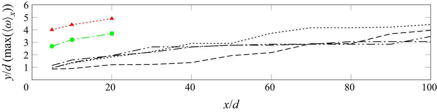
Another related indicator for the differences between spanwise-inclined and normal jets is the wall-normal position of the jet-induced vortex core (see figure 18). It is lower than the penetration depth (see figure 12), as the vortex core lies beneath the upper edge of the vortex. As mentioned earlier, jet/jet interactions do not modify the penetration properties for perpendicular injection (see Ali & Alvi Reference Ali and Alvi2015). For inclined injection, however, the vortex core moves towards the wall ( $y\approx 3d$ for
 $x\geq 40d$ in case D8) due to the jet/jet interactions among adjacent asymmetric vortices, which induce a stronger downwash. This downwash enhances the transfer of momentum to the near-wall region, resulting in more favourable conditions to resist flow separation than for normal injection.
Wall-normal position of the vortex core for ( $\cdots$) D32, (–
 $\cdot \cdot$ –) D16; (–
 $\cdot$ –) D8, (– – –) D4. Normal injection data from Ali & Alvi (Reference Ali and Alvi2015): red triangles and green circles are for intermediate and large spacings, respectively.

4.5. Turbulent boundary-layer statistics
In view of separation-control applications, the influence of jet spacing in AJVG arrays on the boundary-layer and turbulence statistics is of great interest. For separation control, an AJVG array would be placed about  $O(10\delta _{99})$ upstream of the separation region (see e.g. Szwaba Reference Szwaba2005). Ramaswamy & Schreyer (Reference Ramaswamy and Schreyer2021) used an upstream distance of
 $7.69\delta _{99}$. Therefore, we discuss the effects of jet injection on the boundary layer up until this location – where it would interact with a separation-inducing shock wave.
Neighbouring jets and jet-induced structures interact when the jet spacing is reduced to a distance about one order of magnitude larger than the injection pipe diameter. These interactions modify the flow topology and enhance the momentum transfer across the boundary layer, thus making it less susceptible to separation. When the spacing is reduced further, the jet/jet interactions strengthen, which counteracts the effects beneficial for separation control and eventually leads to a secondary flow along the direction of injection.
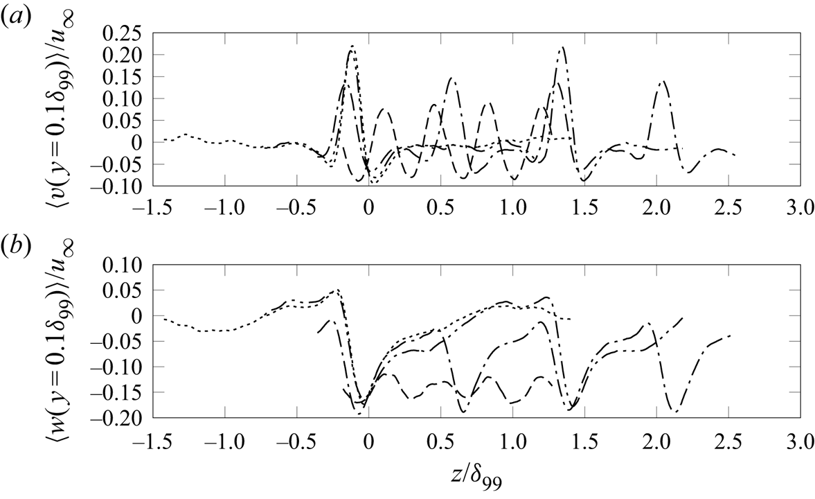
Due to the effects of the major CVP, the direction of the wall-normal and spanwise velocity components changes along the span of the jet array. Between neighbouring vortex pairs, upwash is created (see e.g. the positive peak of the wall-normal velocity for case D32 at  $z=-0.1\delta _{99}$ in figure 19a). The wall-normal velocity distribution at
 $y=0.1\delta _{99}$ and
 $x=\delta _{99}$ in the vicinity of the vortex pair resembles a sinc function with one secondary lobe on either side of the upwash region (see figure 19a), where the wall-normal velocity component is negative due to the downwash induced by the major CVP. The secondary lobe related to the CR vortex is stronger than the one related to the CCR vortex, which indicates a stronger associated downwash (see also Sebastian et al. Reference Sebastian, Lürkens and Schreyer2020). This asymmetry is also observed in the induced spanwise velocity component, where the region of negative velocity corresponding to the CR major vortex is stronger than the region of positive velocity associated with the CCR major vortex (see figure 19b). For D8 and D4, the spanwise velocity component is never positive at the locations shown in figure 19(b). This behaviour is related to excess momentum introduced by the spanwise-inclined jet injection: the momentum coefficient
 $C_\mu$ increases by one order of magnitude (from 0.00792 to 0.06336) when the jet spacing is reduced from
 $32d$ to
 $4d$ (see table 2). The above discussed mechanism effecting a change in spanwise flow direction still manifests itself in alternating velocity magnitudes.
Time-averaged spanwise distribution of (a)  $\langle v\rangle$, and (b)
 $\langle w\rangle$, at
 $x=\delta _{99}$ and
 $y=0.1\delta _{99}$, for cases (
 $\cdots$) D32, (–
 $\cdot \cdot$ –) D16, (–
 $\cdot$ –) D8, (– – –) D4.

Also, the degree of interaction between neighbouring jets is visible in figure 19: for D32 and D16, the flow modifications discussed above diminish to either side of the major CVP. For D8, the patterns come closer together and neighbouring downwash regions merge as the CR vortex draws in the CCR vortex of the respective neighbouring major CVP (as discussed in detail on the basis of figure 15). This effect also contributes to the observed larger regions of negative spanwise velocity (figure 19b). Upon further reduction of the jet spacing to D4, the wave pattern becomes symmetric due to incompletely formed major CVPs.
4.5.1. Direct vicinity of jet injection
Mean velocity profiles across the boundary layer at two spanwise locations are discussed hereinafter to follow directly the downstream effects of the major CVP: the respective locations of the core of the major CVP and midway between two adjacent CVPs.
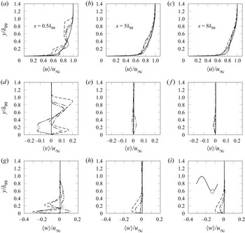
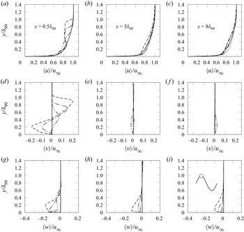
Conditional averages at the centre of the major CVP and halfway between neighbouring major CVPs (see figures 20 and 21, respectively) were computed using the spanwise density distribution. Low-density regions indicate the location of the major CVP (see figure 6). A cosine was fitted on the spanwise density distribution, guaranteeing phase-lock at the local minima. The troughs and crests of the fitted curve at each surveyed streamwise location were then used for conditional or phase averages at the locations of the major CVP and halfway between adjacent major CVPs.
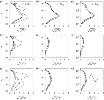
Conditional time-averaged velocity profiles normalized with  $u_{\infty }$ along the core of the major CVP:
 $\langle u\rangle$ (a–c),
 $\langle v\rangle$ (d–f), and
 $\langle w\rangle$ (g-i) at
 $x=0.5\delta _{99}$ (a,d,g),
 $5\delta _{99}$ (b,e,h), and
 $8\delta _{99}$ (c,f,i), for (—) SFP, (
 $\cdots$) D32, (–
 $\cdot \cdot$ –) D16, (–
 $\cdot$ –) D8, (– – –) D4.

Conditional time-averaged velocity profiles of  $\langle u\rangle$ (
 $a$–
 $c$),
 $\langle v\rangle$ (
 $d$–
 $f$), and
 $\langle w\rangle$ (
 $g$–
 $i$) halfway between adjacent major CVPs, for (—) SFP, (
 $\cdots$) D32, (–
 $\cdot \cdot$ –) D16, (–
 $\cdot$ –) D8, (– – –) D4 at
 $x=0.5\delta _{99}$ (a,d,g),
 $5\delta _{99}$ (b,e,h), and
 $8\delta _{99}$ (c,f,i).

The boundary layer in the direct vicinity of injection is modified strongly for all jet spacings (see figures 20a,d,g), but the effect strengthens with decreasing spacing.
The streamwise component features multiple inflection points (see figure 20a). For D32 and D16, the profiles collapse. For D8 and D4, the intensity maxima and minima at  $y/\delta _{99}\approx 0.18$ and 0.37 are shifted to increasingly lower velocities. At
 $y/\delta _{99}\approx 0.37$, the local maximum reaches the value of the uncontrolled profile. The outer part of the boundary layer (
 $y/\delta _{99}>0.4$) is disturbed more strongly for D4, and the effect of jet injection is visible up to
 $y=\delta _{99}$ (versus
 $y\leq 0.85\delta _{99}$ for all other cases). Between the CVPs (see figure 21a), the profiles in the inner region of the boundary layer (
 $y/\delta _{99}<0.4$) deviate only weakly from the undisturbed case. Stronger spacing effects occur in the outer region: for closely spaced jets (D4), the profile deviates equally strongly from the uncontrolled case as at the CVP core location. For D8, the streamwise velocity is decreased between
 $y/\delta _{99}=0.4$ and
 $y/\delta _{99}=0.8$. For D16, the boundary layer is slightly destabilized and the streamwise component is decreased up to
 $y/\delta _{99}<0.65$; for D32, the influence of the jets has decayed at the mid-plane between jets.
The upwash and downwash induced by the major CVP shows in the wall-normal velocity profiles for cases D8 and D4: at  $x=0.5\delta _{99}$, at the CVP core location (see figure 20d), the wall-normal velocities are positive in the inner region of the boundary layer (
 $y\leq 0.4\delta _{99}$), whereas between major CVPs (see figure 21d), negative wall-normal velocities occur. For larger jet spacings (D32 and D16), the CR major vortex causes negative wall-normal velocities in the near-wall region around the vortex core. The profiles for D32 and D16 collapse across the boundary layer, emphasizing the similarity of the induced structures (see also figure 14a). Halfway between adjacent major CVPs, the effect of the jets diminishes: the wall-normal velocity for D32 is negligible, and for D16, a weak positive wall-normal velocity contribution (approximately
 $0.1u_\infty$) occurs at
 $y=0.4\delta _{99}$. Positive wall-normal velocities in the outer layer are related to the CCR major vortex (see figure 20d).
4.5.2. Downstream boundary layer
At  $x=5\delta _{99}$, at the core location of the major CVP, the direct influence of the momentum redistribution by each individual major CVP increases the fullness of the profiles in the near-wall region for cases D32 and D16 (see figure 20b). Farther downstream, jet/jet interaction effects become more important and superimpose the effects of the individual jets: at
 $x=8\delta _{99}$ (figure 20c), case D32 shows similar behaviour as at
 $x=5\delta _{99}$, whereas the velocity profiles for D16 and D8 are fuller in the near-wall region, and case D4 causes a velocity deficit. At the centre location between two major CVPs, the profiles for D32, D16 and D8 collapse and are fuller than in the uncontrolled boundary layer (see figure 21b). Farther downstream (
 $x=8\delta _{99}$), changes are observed only for cases D16 and D8: the profiles become less full than at
 $x=5\delta _{99}$, due to the transfer of momentum from either side of the major CVP.
While cases D32, D16 and D8 follow trends according to the spanwise spacing, a distinctly different behaviour, and a velocity deficit, is observed for D4. D4 has a larger momentum influx per unit length in the spanwise direction (see §§ 4.3 and 4.4) and strong jet/jet interactions, which induce a strong spanwise velocity component (see figures 20h–i and 21g–i) and finally a secondary flow in the direction of injection. These phenomena prevent the full formation of a major CVP that persists for a large streamwise distance and thus lead to a weaker momentum transfer downstream than for the other cases.
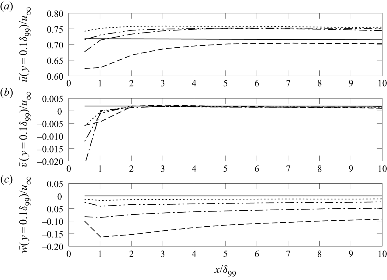
The magnitude of this secondary spanwise flow is almost constant along the span. It persists for at least  $8\delta _{99}$ downstream of injection, and decreases slowly with downstream distance (see also figure 22c). A spanwise flow of increasingly small magnitude also occurs for larger spacings that still allow jet/jet interactions: at
 $x=5\delta _{99}$,
 $\langle w\rangle \approx 0.1u_\infty$ and
 $0.05u_\infty$ for D4 and D8, respectively, while
 $\langle w\rangle$ is negligible for D32.
The deficit in the streamwise velocity profiles for cases D8 and D4 at around  $y>0.2\delta _{99}$ (see figures 20c and 21c) is due to the transfer of momentum from the streamwise to the spanwise directions (figures 20i and 21i). For intermediate spacings (case D8), this momentum transfer results in a longer lifespan of the CVP, which eventually forms a fuller, more separation-resistant boundary layer. For smaller jet spacings (D4) and larger
 $C_\mu$ (see table 2), the momentum influx per unit span increases. This additional momentum, combined with the momentum transfer in the crossflow, results in a much stronger secondary flow; also, the direct influence of the CVP for D4 has already decayed upstream of
 $x=5\delta _{99}$ (see the missing contribution of the upwash and downwash in the wall-normal velocity component). These effects make the boundary layer even more susceptible to separation than an uncontrolled flow.
In the wall-normal velocity component, the CVP-induced upwash and downwash are reflected in positive and negative velocities (see figures 20d–f and 21d–f). Here, the influence of the jets reduces significantly already shortly downstream of injection ( $x\leq 2\delta _{99}$; see also figure 22b); evidently, the reduction depends on the degree of jet/jet interactions and hence the spacing. In the mid-plane between adjacent CVPs (figures 20e,f), an influence, namely a small region of non-zero velocity near the wall, is visible for D8 only several
 $\delta _{99}$ downstream. For D4 and D16, the influence decays quickly, and the large spacing in case D32 prevents any influence in the mid-plane between jets in the first place. These trends indicate that the vortex pair for D16 perishes faster than for D8: vortical structures induced by moderately spaced jets (D8) interact in a way that increases the longevity of the major CVP. The longevity of the jet influence over a wide spanwise region seems to be a key feature for the separation-control effectiveness of air-jets.
Streamwise evolution of time- and spanwise-averaged velocities (a)  $\bar {u}$, (b)
 $\bar {v}$, and (c)
 $\bar {w}$, at
 $y=0.1\delta _{99}$: (—) SFP, (
 $\cdots$) D32, (–
 $\cdot \cdot$ –) D16, (–
 $\cdot$ –) D8, (– – –) D4.

The downstream evolution of time- and spanwise-averaged velocities at  $y=0.1\delta _{99}$ (located in the near-wall region where the streamwise velocity profile is fuller than in an uncontrolled flow for some cases) is shown in figure 22. In the vicinity of injection, the streamwise component initially decreases (most strongly for the smallest jet spacings). It then increases and remains at a constant high level for all spacings except D4, indicating fuller profiles and thus a more separation-resistant boundary layer for an extended downstream distance. Without jet injection, the streamwise velocity is about
 $0.718u_\infty$ at
 $y=0.1\delta _{99}$; for D32, D16 and D8,
 $\bar {u}(y=0.1\delta _{99})\approx 0.75u_\infty$ for
 $x>\delta _{99}$, with only minor differences between the cases. For D4, a velocity deficit occurs over the entire streamwise extent that we considered. The standard deviations of the time-averaged velocities show a similar convergent behaviour (not shown). All components are highest in the vicinity of injection and decrease quickly downstream, reaching a constant level for
 $x\geq 2\delta _{99}$. They are largest for D8, which is related to the spanwise waviness of the velocity components. This behaviour is caused by the favourable jet interactions, which result in enhanced momentum redistribution across the boundary layer. The standard deviation, and thus the activity in the near-wall region, is lowest for D4.
The major CVP also leaves a clear footprint in the turbulent velocities (see the conditionally/phase averaged r.m.s. velocity profiles – normalised with the friction velocity  $u_\tau$ and length scale
 $l_\tau$ of the uncontrolled case SFP – shown in figures 23 and 24). At the location of the major CVP core, a distinct outer-layer peak develops for all velocity components (at around
 $y^+\approx 200$ close to the injection location at
 $x=0.5\delta _{99}$; figures 23a,d,g). In the downstream evolution, this peak dissipates and shifts away from the surface, from
 $y^+\approx 200$ at
 $x=0.5\delta _{99}$ to
 $y^+\approx 800$ at
 $x=8\delta _{99}$ (see figure 23).
Conditional time-averaged r.m.s. velocity statistics:  $\sqrt{\langle{u'^2}\rangle}^+$ (a–c),
 $\sqrt{\langle{v'^2}\rangle}^+$ (d–f), and
 $\sqrt{\langle{w'^2}\rangle}^+$ (g–i), along the core of a major CVP, for (—) SFP, (
 $\cdots$) D32, (–
 $\cdot \cdot$ –) D16, (–
 $\cdot$ –) D8, and (– – –) D4, at
 $x=0.5\delta _{99}$ (a,d,g),
 $5\delta _{99}$ (b,e,h), and
 $8\delta _{99}$ (c,f,i).

Conditional time-averaged r.m.s. velocity statistics:  $\sqrt{\langle{u'^2}\rangle}^+$ (a–c),
 $\sqrt{\langle{v'^2}\rangle}^+$ (d–f), and
 $\sqrt{\langle{w'^2}\rangle}^+$ (g–i), halfway between adjacent major CVPs, for (—) SFP, (
 $\cdots$) D32, (–
 $\cdot \cdot$ –) D16, (–
 $\cdot$ –) D8, and (– – –) D4, at
 $x=0.5\delta _{99}$ (a,d,g),
 $5\delta _{99}$ (b,e,h), and
 $8\delta _{99}$ (c,f,i).

The jets also amplify the near-wall peak in the buffer layer related to the wall turbulence ( $x=0.5\delta _{99}$). The buffer-layer peak decreases in the downstream evolution, and the conventional wall turbulence distribution recovers. At spanwise locations between adjacent CVPs, this bimodal behaviour is observed only for cases D4 and (to a weaker extent) D8 due to the strong interactions at small jet spacings (see figure 24).
4.5.3. Region where the separation shock would be encountered in control applications
In the accompanying experimental investigations (see § 3 and Ramaswamy & Schreyer Reference Ramaswamy and Schreyer2021), an AJVG array is installed approximately  $8\delta _{99}$ upstream of a compression–ramp interaction. To better understand the flow encountered by the ramp-induced shock wave, as well as upcoming interactions, we document and discuss the flow in this region. Time-averaged streamwise velocity contours in the spanwise/wall-normal plane at
 $x=8\delta _{99}$ are shown in figure 25, superimposed with contour lines of
 $\langle u\rangle /u_\infty =0.99$, 0.9, 0.8, 0.7 and
 $0.6$, and the
 $\langle v\rangle -\langle w\rangle$ vectors. For cases D32 and D16, individual circular CR major vortices with diameters of approximately
 $\delta _{99}$ occur. The vortex cores are located at about
 $y=0.4\delta _{99}$. The downwash effect due to the major vortex that makes the boundary layer less susceptible to separation (especially on the side opposite to the direction of injection; Sebastian et al. Reference Sebastian, Lürkens and Schreyer2020) thus is still active.
Contours of the streamwise velocity component, superimposed with contour lines (white) for  $\langle u\rangle /u_\infty =0.99$, 0.9, 0.8, 0.7 and
 $0.6$ at
 $x=8\delta _{99}$: (a) D32, (b) D16, (c) D8, (d) D4.

Jet interactions at the reduced spacing  $D=8d$ lead to smaller, merging vortices (
 $\approx 0.7\delta _{99}$), where the CR major vortices draw in the CCR vortex of the respective adjacent pair. The contour lines are nonlinear and wave-like. For D4, jet-induced vortical structures are no longer visible at
 $x=8\delta _{99}$ due to the increased
 $C_\mu$ and momentum influx per unit span. This increase eventually prevents the formation of vortices and results in a secondary flow in the jet-injection direction (see also figures 16 and 22).
Compared with the uncontrolled case (SFP), the time-averaged streamwise velocity at  $y=0.1\delta _{99}$ is increased by approximately 5 % and 10 % on the side towards which the jets are injected and opposite to it, respectively, for D32 and D16 (see figure 26a). For D8, the uniform spanwise wave pattern induced by the interaction between jet-induced structures (see also figures 6 and 19) persists even this far downstream of injection. Unlike for D32 and D16, the region with higher streamwise velocity for D8 is confined locally to areas where the CR major vortex is present. This behaviour is also visible in the streamwise/spanwise Mach number distribution (see figure 10c). The increased susceptibility of the flow to separation at narrow jet spacing (D4) prevails far downstream of injection: the streamwise velocity component is still smaller than in the undisturbed case (see figure 26a).
(a) Spanwise distribution of the time-averaged streamwise velocity. (b,c) Time- and spanwise-averaged streamwise velocity plotted versus  $y/\delta _{99}$ and, van Driest-transformed, versus
 $y^+$, respectively, at
 $x=8\delta _{99}$. Here, (—) SFP, (
 $\cdots$) D32, (–
 $\cdot \cdot$ –) D16, (–
 $\cdot$ –) D8, (– – –) D4.

The observed trends to fuller profiles or velocity deficit – in spanwise-varying intensity – are strong enough to be visible in time- and spanwise-averaged velocity profiles (see figures 26b,c). The growth rate of the boundary layer is not affected by the jets. The overall thickness  $\delta _{99}$ of the boundary layer, however, shows minor increases of 5 % and 7 % for D32 and D8, respectively, and for D4, the thickness increases considerably, by 25 % compared with case SFP (not shown here). The jet-induced changes affect only the inner region of the boundary layer (
 $y<0.6\delta _{99}$); farther away from the surface, the profiles collapse. These effects appear more clearly in the mean velocity scaled according to van Driest (see figure 26c, where the wall-normal distance is scaled with the viscous length scale of the unperturbed case SFP). With jet injection, the profile becomes less steep in the viscous sublayer. In the viscous sublayer and buffer layer, cases D32, D16 and D8 collapse, and the profile for D4 is even less steep. In the log-layer, the profiles for D32, D16 and D8 are fuller, with a higher log-law constant, whereas D4 collapses with the undisturbed case.
4.6. Dominant dynamic modes and governing mechanisms
Phenomena relevant to the dynamic behaviour of the flow for the different jet spacings were extracted from sequences of instantaneous fields of  $p$,
 $\rho$,
 $u$,
 $v$ and
 $w$ using dynamic mode decomposition (DMD). DMD extracts the spatial representations and associated characteristic frequencies of dynamically relevant modes from a time-resolved data sequence (Rowley et al. Reference Rowley, Mezić, Bagheri, Schlatter and Henningson2009; Schmid Reference Schmid2010). To select the most dominant modes, we used the sparsity-promoting mode-selection algorithm SPDMD of Jovanović, Schmid & Nichols (Reference Jovanović, Schmid and Nichols2014). The method computes an optimization problem for the detection of a subset of features that optimally approximate the original flow field. The SPDMD algorithm effectively differentiates the dominant structures from the less relevant ones. Moreover, modes with decay rates close to zero are only considered to limit the selection to quasi-steady modes.
The purpose of this analysis is twofold: (a) it allows us to understand the flow dynamics and thus helps to explain the previously observed increasing or decreasing control effectiveness, which ultimately enables the design of effective control set-ups; and (b) it allows us to identify the characteristic frequencies for jet configurations with different degrees of interaction, which is necessary in view of the selection of forcing frequencies for other effective control methods using unsteady, periodically triggered jets in open- or closed-loop control strategies (see e.g. Castelino & Gutmark Reference Castelino and Gutmark2021). We applied 3-D DMD in a spatial subdomain with a streamwise extent  $-1\leq x/\delta _{99} \leq 5$ (
 $-10\leq x/d \leq 50$) on temporal snapshots equispaced in time with
 $\Delta \tilde {t}\,\tilde {u}_\infty /10\tilde {d}=1\unicode{x2013}1.2$ (
 $\Delta \tilde {t}\,\tilde {u}_\infty /\tilde {\delta }_{99}=1\unicode{x2013}1.2$). This sampling interval allows us to extract the low- to medium-frequency unsteadinesses typically governing separation-bubble dynamics (see e.g. Clemens & Narayanaswamy Reference Clemens and Narayanaswamy2014). It has been verified that reducing the sampling frequency does not affect the low-frequency modes; they are not biased by aliasing errors. Moreover, resolving turbulence only partially has favourable effects on the signal-to-noise ratio and convergence (Nichols et al. Reference Nichols, Larsson, Bernardini and Pirozzoli2017).
For a single inclined jet in supersonic crossflow, four dynamic mechanisms dominate: low-frequency motions of the jet-induced bow and envelope shocks; vortex generation and interactions between vortical structures in the wake of the jet; the associated momentum redistribution in the downstream crossflow; and interactions between the boundary-layer turbulence and shocks (see Sebastian et al. Reference Sebastian, Lürkens and Schreyer2020). Multiple modes with similar spatial representations and characteristic frequencies contribute to each of these features (see table 5). Case D32 in the present study essentially corresponds to this single-jet case.
Characteristic frequencies of the selected dynamic modes for different jet spacings. Results for case D32 are from Sebastian et al. (Reference Sebastian, Lürkens and Schreyer2020).

When jets are installed in a line array, the same modes remain relevant for all jet spacings. With decreasing spacing and thus increasing interactions between the jet-induced structures, the low-frequency bow-shock oscillations that cause flow modulation and vortex generation shift to a lower frequency, though. Additional modes are superimposed when jet/jet interactions increase. The modes governing the flow dynamics in cases D4–D32 are summarized in table 5 along with the respective characteristic frequencies. Detailed descriptions of the dynamic behaviour of the flow fields associated with cases D16, D8 and D4 follow in §§ 4.6.1, 4.6.2 and 4.6.3, respectively.
4.6.1. Large spacing with negligible jet/jet interactions (Case D16)
The 3-D DMD analysis for case D16 was performed using 180 instantaneous snapshots with a time interval  $\Delta \tilde {t}\,\tilde {u}_\infty /10\tilde {d}=1.18$, which yields a resolvable Strouhal number range
 $St=\tilde {f}\tilde {d}/\tilde {u}_\infty ={0.00024}\unicode{x2013}0.0424$. The equivalent Strouhal numbers based on boundary-layer thickness (
 $St_{\delta _{99}} = \tilde {f}\tilde {\delta }_{99}/\tilde {u}_\infty = 10\,St$) are
 ${0.0024}\leq St_{\delta _{99}}\leq 0.424$.
In the corresponding DMD spectrum (figure 27), circles denote DMD modes and red + symbols mark the subset of modes detected using SPDMD. The major dynamic behaviour of the flow field is captured with four representative modes from this subset (marked with filled blue squares in the inset in figure 27). The eigenvalues and characteristic frequencies of the selected modes ( $\varPhi _1$–
 $\varPhi _4$) are:
 $\lambda (\varPhi _1)=(-0.00086+0.01238{\rm i})$,
 $St_{\varPhi _1}=0.0015$;
 $\lambda (\varPhi _2)=(-0.00081+0.01701{\rm i})$,
 $St_{\varPhi _2}=0.0021$;
 $\lambda (\varPhi _3)=(-0.00055+0.04049{\rm i})$,
 $St_{\varPhi _3}=0.0055$; and
 $\lambda (\varPhi _4)=$
 $(-0.00046+0.11015{\rm i})$,
 $St_{\varPhi _4}=0.0137$. Modes enclosed within each dashed-line rectangle in figure 27 share similar spatial representations and characteristic frequencies, and thus contribute to the same dynamic behaviour. The modes and overall behaviour are very similar for cases D16 and D32, since the jet spacings in both cases are so large that adjacent CVPs do not interact to a significant extent.
DMD mode spectrum for D16. Inset: most relevant modes. Red ‘+’ symbol: modes detected with SPDMD. Filled squares: modes selected for further analysis.

The low-frequency modes  $\varPhi _1$ and
 $\varPhi _2$ correspond to the streamwise shock dynamics, flow modulation, and subsequent vortex generation. Mode
 $\varPhi _1$ is visualized using pressure fluctuations in figure 28(a): the bow, envelope and barrel shocks are clearly recognizable. Strong pressure fluctuations in the region between the bow and barrel shocks indicate vortex shedding from the windward side of the barrel shock. Bow-shock oscillations in the spanwise direction cause flow modulation and momentum transfer, resulting in fuller boundary-layer profiles on the side opposite to the jet-injection direction (see Sebastian et al. Reference Sebastian, Lürkens and Schreyer2020).
Visualizations of modes (a)  $\varPhi _1$ using pressure fluctuations, and (b)
 $\varPhi _4$ using streamwise velocity fluctuations, in a streamwise/wall-normal plane along the jet centreline for case D16.

The moderate frequency mode  $\varPhi _3$ (
 $St=0.0055$, not shown) is related to the vortex interactions in the jet wake as the upper-trailing vortex merges with the CCR major vortex to form an uneven pair of counter-rotating vortices (see also figure 14a and Sebastian et al. Reference Sebastian, Lürkens and Schreyer2020). The medium frequency mode
 $\varPhi _4$, visualized with the streamwise velocity in figure 28(b), corresponds to a wrinkling of the bow shock that is related to interactions between the boundary-layer turbulence and the shock wave. Similar behaviour has been observed for SWBLI (Pasquariello, Hickel & Adams Reference Pasquariello, Hickel and Adams2017).
4.6.2. Jet spacing with jet/jet interactions favourable for separation control (case D8)
The 3-D DMD for case D8 was performed with 206 instantaneous snapshots equispaced in time with  $\Delta \tilde {t}\,\tilde {u}_\infty /10\tilde {d}=1.12$, thus resolving frequencies with
 $0.00022 \leq St \leq 0.045$.
For this case, a slightly larger number of modes is required to represent the major dynamics of the flow. Six representative modes from the subset of modes identified using SPDMD are (see figure 29a):  $\lambda (\varPhi _1)=(-0.00141+0.00865{\rm i})$,
 $St_{\varPhi _1}=0.0011$;
 $\lambda (\varPhi _2)=(-0.00097+0.01264{\rm i})$,
 $St_{\varPhi _2}=0.0016$;
 $\lambda (\varPhi _3)\!=\!(-0.00078+0.04204{\rm i})$,
 $St_{\varPhi _3}\!=\!0.0052$;
 $\lambda (\varPhi _4)=(-0.00073+0.06841{\rm i})$,
 $St_{\varPhi _4}=0.0085$;
 $\lambda (\varPhi _5)=(-0.00062+0.15541{\rm i})$,
 $St_{\varPhi _5} = 0.0195$; and
 $\lambda (\varPhi _6)=(-0.00079+0.18419{\rm i})$,
 $St_{\varPhi _6}=0.0230$.
DMD spectrum of cases (a) D8 and (b) D4. See figure 27 for symbols.

As for D32 and D16, the low-frequency modes ( $\varPhi _{1}$ and
 $\varPhi _{2}$) are related to the shock motions, subsequent flow modulation and vortex generation, and medium-frequency modes (
 $\varPhi _{5}$ and
 $\varPhi _{6}$) capture interactions between the boundary-layer turbulence and shock structures.
Modes  $\varPhi _{1}$ and
 $\varPhi _{2}$ have spatial representations similar to those for cases D32 and D16 (see figure 28a). The onset of these flow dynamics, however, is at about 30 % lower frequency than for D32 and D16 (
 $St_{\varPhi _1} = 0.0011$ instead of 0.0015).
Two additional modes ( $\varPhi _{3}$ and
 $\varPhi _{4}$) become important for D8. These are thus the mechanisms responsible for the improvement of the control effectiveness: Mode
 $\varPhi _{3}$ is related to interactions between shock structures of neighbouring jets. In the density fluctuation field used to visualize
 $\varPhi _3$, a scallop-shaped pattern represents the interacting shocks (see figure 30a and compare with figure 6c). Shock oscillations cause flow modulation in the spanwise direction (Sebastian et al. Reference Sebastian, Lürkens and Schreyer2020), which, combined with the interactions among the shocks, results in an increased spanwise velocity component (see the spanwise velocity fluctuation field for
 $\varPhi _3$ in figure 30b). Interactions between neighbouring CVPs are also visible as an amplified spanwise velocity fluctuation level in the region between adjacent CVPs in mode
 $\varPhi _4$ (see figure 31a and also figure 15). The described shock/shock interactions and related spanwise flow modulations are similar to the shock dynamics associated with the low-frequency modes. In both cases, flow modulation results in enhanced momentum transfer. At lower frequency, this transfer results in fuller boundary-layer profiles.
Mode  $\varPhi _3$ for case D8, visualized with (a) the pressure fluctuation field, and (b) the spanwise velocity fluctuation field, in a spanwise/wall-normal plane at
 $x=4d$.

Visualizations of (a)  $\varPhi _4$ with spanwise velocity fluctuations, and (b)
 $\varPhi _5$ with density fluctuations, in spanwise/wall-normal planes at
 $x=2.5d$ and
 $x=4d$, respectively, for case D8.

Mode  $\varPhi _5$ covers interactions between the merged shock wave upstream of injection and the boundary-layer turbulence. The mode manifests itself as smeared/disintegrated shock in the spanwise direction (see the visualization using density fluctuations in figure 31b). Similarly, in mode
 $\varPhi _6$, the shock is smeared in the streamwise direction due to shock/turbulence interactions. The
 $\varPhi _6$ dynamics is similar to the dynamics observed for mode
 $\varPhi _4$ in cases D32 and D16 (see figure 28b) and
 $\varPhi _6$ also has a similar spatial representation (not shown).
4.6.3. Small jet spacing with strong jet/jet interactions (case D4)
The DMD for case D4 was performed on 324 instantaneous 3-D flow fields equispaced in time with  $\Delta \tilde {t}\,\tilde {u}_\infty /10\tilde {d}=1.16$. Six representative modes (marked with blue squares in the DMD spectrum in figure 29b) describe the dynamics for this case with very small jet spacing:
 $\lambda (\varPhi _1)=(-0.00082+0.00441{\rm i})$,
 $St_{\varPhi _1}=0.0006$;
 $\lambda (\varPhi _2)=(-0.00038+0.00946{\rm i})$,
 $St_{\varPhi _2}=0.0012$;
 $\lambda (\varPhi _3)=(-0.00020+0.01487{\rm i})$,
 $St_{\varPhi _3} =0.0019$;
 $\lambda (\varPhi _4)=(-0.00022+0.06224{\rm i})$,
 $St_{\varPhi _4}=0.0078$;
 $\lambda (\varPhi _5)=(-0.00018+$
 $0.13402{\rm i})$,
 $St_{\varPhi _5}=0.0167$; and
 $\lambda (\varPhi _6)=(-0.00030+0.14706{\rm i})$,
 $St_{\varPhi _6}=0.0183$.
As for larger spacings, the low-frequency modes ( $\varPhi _{1}$ and
 $\varPhi _{2}$) are linked to the streamwise shock motions and subsequent vortex generation; medium-frequency modes (
 $\varPhi _{5}$ and
 $\varPhi _{6}$) cover shock–turbulence interactions. As in case D8, moderate-frequency modes (
 $\varPhi _3$ and
 $\varPhi _4$) represent interactions among the shock structures and between adjacent CVPs.
The spatial representations of  $\varPhi _{1}$ and
 $\varPhi _{2}$ are very similar to the other cases (see figure 28a) and therefore are not shown. The characteristic frequency of the shock oscillation is even lower than for D8 (
 $St=0.0006$, i.e. about 60 % below D32 and D16, and 50 % below D8). Thus the stronger the jet/jet interactions, the lower the oscillation frequency of the shock.
Mode  $\varPhi _{3}$ captures interactions between neighbouring shocks, manifesting as spanwise pressure fluctuation variations in a merged shock upstream of the jet (see figure 32a). This merged shock is also visible in the density distribution (see figure 6d). Also for these shock-interaction dynamics, the characteristic frequency decreases (about 50 % lower than for D8).
Visualization of modes for D4: (a)  $\varPhi _3$ using pressure fluctuations, and (b)
 $\varPhi _4$ using spanwise velocity fluctuations, in spanwise/wall-normal planes at
 $x=3d$ and
 $x=5d$, respectively. (c,d) Mode
 $\varPhi _5$ using the spanwise velocity and pressure fluctuation fields, respectively, at
 $x=2.5d$.

The dynamic interactions between jets with small spacing appear as spanwise undulations in the spanwise velocity fluctuation component captured by mode  $\varPhi _4$ (see figure 32b). The undulation pattern is also visible in figures 16(a) and 19(b).
The medium-frequency mode  $\varPhi _5$ (
 $St=0.0167$) captures interactions between turbulence and the merged upstream shock. The secondary flow in the spanwise direction and the spanwise wrinkling of the shock upon impingement of turbulent structures from the boundary layer are visible in figures 32(c) and 32(d), respectively. The shock wrinkling also has a streamwise component, which is captured by mode
 $\varPhi _6$ and has a spatial representation similar to that for the corresponding mode
 $\varPhi _4$ for D16 shown in figure 28(b). The observed decrease in control effectiveness for D4 is related mostly to the higher momentum influx and the resulting stronger spanwise velocity component, which inhibit the formation of the major CVP and cause a secondary spanwise flow. Mode
 $\varPhi _5$ represents these flow dynamics.
4.7. Conceptual model of the flow around arrays of spanwise-inclined jets
We summarized the current findings in conceptual models, which are shown in figures 33(a,b) for jet spacings that allow moderate and strong jet/jet interactions, respectively. For large spacings that do not allow for interactions between neighbouring jet-induced structures (D32 and D16), the flow field consists of a spanwise row of independent jet-in-crossflow events as described in Sebastian et al. (Reference Sebastian, Lürkens and Schreyer2020) (see figure 1).
Schematic drawing of the flow around (a) a moderately spaced array of jets (D8), and (b) a closely spaced array of jets (D4).

For moderately spaced jets (e.g. case D8; see figure 33a), the individual bow shocks upstream of each jet start merging and form a scallop pattern (see figure 6). Also, the associated upstream separation regions merge into a wave-like pattern (see figure 9).
When the jets are placed even closer together (e.g. case D4; see figure 33b), the upstream bow shocks of the individual jets merge completely into a common shock front, and the induced upstream separation region increases considerably.
Also, the jet-induced vortex structures interact for small-enough spacings. For single jets and large spacings, the spanwise extent of the CVP saturates to about  $0.6\delta _{99}$ (at
 $x=0.5\delta _{99}$). For moderately spaced jets, the stronger CR vortex draws in the CCR vortex from the adjacent CVP, which leads to a reduced spanwise extent and semi-upright orientation of the major CVP, and enhances vorticity (see figures 15 and 17b). The momentum transfer across the boundary layer increases, making it less susceptible to separation (figures 5d and 26).
When the jet spacing is reduced further, the momentum influx due to injection increases. This effect (a) hinders the major CVP to fully develop, thus forming skewed CVPs of small size ( $0.3\delta _{99}$ at
 $x=0.5\delta _{99}$), and (b) induces a secondary flow in the direction of injection. Consequently, the downstream boundary layer is more susceptible to separation (figure 5e).
5. Conclusions
Jets injected into supersonic crossflows are of great relevance for many engineering applications. For the control of shock-induced separation, for example, rows of spanwise-inclined jets are very effective while also reducing the associated parasitic drag compared with other methods. The inter-jet spacing within the row of jets has been observed to affect the control efficiency. To understand the flow physics behind this effect, we performed large-eddy simulations of the spanwise injection of a row of jets inclined to the surface by  $45^\circ$ with four different jet spacings. A turbulent boundary layer on a flat plate at
 $M_\infty =2.5$ and
 $Re_{\theta }=7000$ served as crossflow. The jets were injected from circular orifices with diameter
 $d=0.1\delta _{99}$. Arrays with jet spacings
 $D=32d, 16d, 8d, 4d$ were studied. The jets were supplied with air at stagnation conditions from a plenum within the flat plate.
The influence of jet spacing on the boundary layer and the introduced flow structures was studied by analysing the flow topology, vortical structures and turbulent boundary-layer statistics. To analyse the governing dynamic mechanisms relevant in each case, we applied 3-D dynamic mode decomposition. Also, in view of future studies on control and effective mixing with periodically forced jets, the gained knowledge on jet dynamics and natural frequencies is crucial for the selection of suitable forcing frequencies.
The current study revealed different jet/jet interactions and their effects on the downstream flow. The jet-induced major vortex pair is the dominant flow structure responsible for energizing the near-wall boundary layer. Interactions among adjacent vortex pairs vary depending on the jet spacing. Consequently, the momentum transfer, and eventually the control efficiency, are influenced: interactions of suitable strength increase and stabilize the major CVP, while too-strong interactions prevent the CVPs’ full formation.
The injected jets induce local separation regions, shocks and vortex structures in the crossflow. For large spacings, individual bow shocks form upstream of each jet. With decreasing spacing, the shock angles steepen and the shocks merge first into a scallop pattern and then into a joint shock front with a larger standoff distance. Also, the separation regions forming upstream of each jet move closer together when the jet spacing is reduced, and merge eventually. For intermediate spacings ( $D=8d$), the upstream separation line is corrugated; for very narrow spacings (
 $D=4d$), the upstream separations have fully merged; the bubble is flatter and extends farther upstream.
The merged shock front for small jet spacings presents a larger obstacle to the oncoming crossflow; consequently, the jet penetration depth is larger. Even for small spacings, however, the outer part of the boundary layer is only weakly disturbed, which implies low associated parasitic drag (also lower than for perpendicularly injected jets).
Spanwise-inclined jets introduce asymmetrical vortex structures into the boundary layer, of which the major CVP is most relevant for control applications.
When the jet spacing is around  $10d$, the jets interact with beneficial effects. The stronger CR major vortex draws in the CCR vortex of the neighbouring CVP, thus consuming the vorticity of this vortex. A stronger CR vortex forms, which persists for a longer downstream distance and enhances the momentum transfer across the boundary layer. Due to the longevity of the vortical structures, the boundary-layer profiles become fuller for a longer downstream distance, and the boundary layer is more resistant to separation.
When the jet spacing is decreased too much, strong interactions obstruct the development of the major CVP. Furthermore, the surplus of momentum influx due to injection causes the formation of a spanwise secondary flow in the direction of injection. The streamwise momentum from the outer part of the boundary layer is mainly transferred to the spanwise secondary flow, causing large streamwise velocity deficits in the outer region. These effects make the boundary layer even more susceptible to separation than an uncontrolled flow.
The better separation-control effectiveness of rows of spanwise-inclined jets compared with perpendicular injection is related to several aspects. For wall-normal injection, the jet spacing does not modify the jet penetration and liftoff of the symmetric CVPs. For spanwise-inclined injection, interactions among the adjacent asymmetric CVPs increase the downwash, which delays the vortex liftoff. Consequently, the transfer of momentum into the near-wall region is enhanced, which increases the ability to resist flow separation.
Detailed insight into the dynamic mechanisms governing the flow was obtained from 3-D dynamic mode decomposition. A number of modes – governing low-frequency motions of the shocks, the vortex generation and interactions between vortices in the wake of the jet, and the associated momentum redistribution in the flow, as well as shock/turbulence interactions – are common to all spacing cases and even single inclined jets. When the jet/jet interactions strengthen, the low-frequency bow-shock oscillation and the associated flow modulation and vortex generation shift to a lower frequency range, and additional modes become relevant. For both moderately and closely spaced jets, moderate-frequency modes related to interactions among the shock structures and between adjacent CVPs are superimposed. The shock–turbulence interaction disintegrates the merged shock in both the spanwise and streamwise directions. For the smallest spacing, one further mode related to the spanwise secondary flow contributes significantly to the flow dynamics. This mode is co-responsible for the decreased control effect (along with the incomplete formation of the major CVPs).
Acknowledgements
We would like to thank the High-Performance Computing Center Stuttgart and the Jülich Supercomputing Center for providing the computational resources within a large-scale project of the Gauss Center for Supercomputing. We also thank D.P. Ramaswamy for sharing the experimental data.
Funding
This work was supported by the Deutsche Forschungsgemeinschaft within the framework of the Emmy Noether Programme (grant SCHR 1566/1-1).
Declaration of interests
The authors report no conflict of interest.