I. INTRODUCTION
The yield behavior of solid polymers is sensitive to hydrostatic pressure. It is evident that the von Mises' and Tresca's yield criteria, which were formulated by assuming that the yielding is independent of hydrostatic pressure, are inapplicable to polymers. Previous studiesReference Mears, Pae and Sauer1–Reference Quinson, Perez, Rink and Pavan6 have shown that the yield strength increases approximately linearly with the hydrostatic pressure. The Drucker–PragerReference Drucker and Prager7 yield criterion which takes into account the linear dependence of the yield strength on hydrostatic pressure is usually adopted and is shown below:
 $$f\left( {{\sigma _{ij}}} \right) = \bar \sigma -\left( {{\sigma _{{\rm{y}}0}} + kP} \right) = 0\quad {\rm{,}}$$
where 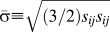 $\bar \sigma \equiv \sqrt {\left( {{3 \mathord{\left/ {\vphantom {3 2}} \right. \kern-\nulldelimiterspace} 2}} \right)s_{ij} s_{ij} }$ is the effective stress; σy0 is the yield strength under the pure shear deformation; k is the coefficient of internal friction, which reflects the effect of the hydrostatic pressure on the yield strength; P ≡ −σii/3 is the hydrostatic pressure. To evaluate the effect of hydrostatic pressure on the yield strength, uniaxial tension or compression at various hydrostatic pressures was carried out to determine the coefficient of internal friction, k, for bulk polymers.Reference Mears, Pae and Sauer1,Reference Sauer, Mears and Pae8–Reference Bardia and Narasimhan10 However, with the development of micromachining process, polymeric moldings and structures become smaller and smaller. The conventional testing techniques face great challenges when applied to such products due to the difficulty of specimen preparation. Consequently, there is an increasing demand for new techniques to evaluate the effect of hydrostatic pressure on the yield strength for small polymeric products.
Instrumented indentation, which is also well known as depth-sensing indentation and nanoindentation, is one of the most promising techniques for probing mechanical properties of small volumes of material such as thin films deposited on substrates and small structures such as micro-electro-mechanical-systems (MEMS), because the tests are conducted in a small region (typically 1–10 μm in diameter) on the surface of actual components with little specimen preparation. Unlike conventional tensile and compressive tests, determination of mechanical properties using instrumented indentation needs to know some background knowledge of the material behavior. Great efforts have been made to relate the mechanical properties to the indentation data to extract the corresponding mechanical properties of indented materials. For example, Oliver and PharrReference Oliver and Pharr11 developed a widely accepted method to determine elastic modulus for elastic–plastic solids by relating elastic modulus to the initial unloading stiffness and the projected contact area. Similarly, by establishing the correlations between the plastic properties and the indentation data, indentation methods for characterization of the yield response of elastic-power law hardening solids were proposed.Reference Dao, Chollacoop, Vliet, Venkatesh and Suresh12–Reference Cao, Qian, Lu and Yao17
The indentation responses of solid polymers have also been studied.Reference Oyen and Cook18–Reference Seltzer, Cisilino, Frontini and Mai23 Not only time-independent elastic–plastic deformation, but also time-dependent viscoelastic deformation occurs during indentation tests. Due to the complexity of the deformations, researchersReference Zhang, Zhang, Zeng and Shen19–Reference Peng, Feng, Huan and Zhang22 usually isolate the elastic, plastic, and viscoelastic deformations and determine the corresponding material properties individually. Generally, the fast loading and unloading load–depth curve is used to determine the time-independent elastic–plastic properties, and the time-dependent viscoelastic properties are extracted from the holding segment of the load–depth curve, because the time-independent elastic–plastic deformation is dominant in the fast loading and unloading segments and the time-dependent viscoelastic deformation is the primary deformation occurs during holding. To reduce the difficulty of analysis while retaining the important features of indentation responses for polymers, both the strain softening and strain hardening after yielding are usually neglected. Based on the assumption that the solid polymers display an elastic-perfectly plastic behavior and that the yield behavior obeys the Drucker–Prager yield criterion, Seltzer et al.Reference Seltzer, Cisilino, Frontini and Mai23 presented an indentation method to determine the Drucker–Prager parameters using Berkovich and spherical indenters.
In the present work, assuming the behavior of solid polymers can be approximated by an elastic-perfectly plastic description during fast loading and considering the linear dependence of the yield strength on hydrostatic pressure, two dimensionless functions were constructed to characterize the instrumented sharp indentation by dimensional analysis. With the aid of finite element analysis, two analytical expressions that relate the indentation data to the plastic properties were derived from the dimensionless functions. The coefficient of internal friction, k, that reflects the effect of hydrostatic pressure on the yield strength was then extracted from the indentation curve using these two analytical expressions. Experiments were carried out on bulk polypropylene (PP), polycarbonate (PC), and unplasticized polyvinyl chloride (UPVC) to verify the reliability of the newly presented method.
II. METHODS
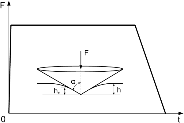
To evaluate the effect of hydrostatic pressure on the yield strength, a sharp indenter (conical, Berkovich or Vickers) indenting normally into solid polymers with an approximate step-hold-unload loading profile (see Fig. 1) was considered. As we know, the viscous or time-dependent properties are important characteristics of polymers. However, to reduce the difficulty of dimensional analysis while retaining the important features of indentation responses, we ignored the effects of the viscous properties. This is reasonable because the analysis was based on a specified loading profile, namely, an approximate step-hold-unload loading profile. According to Oyen's work,Reference Oyen24 the viscous effects during the approximate step loading segment are negligible so long as the loading time is about one-tenth of the dominant retardation time. During the long-time holding, the viscous deformation occurs sufficiently, so that the viscous deformation occurs during the unloading segment can be neglected. Feng and NganReference Feng and Ngan25 proposed a “creep factor” to help decide whether the holding is long enough for ignoring the viscous effects. The creep factor, f c, is defined as
 $${f_{\rm{c}}} = {{{{\dot h}_{\rm{h}}}S} \over {\left| {{{\dot F}_{\rm{u}}}} \right|}}\quad {\rm{,}}$$
where  ${\dot h_{\rm{h}}}$ is the creep rate (dh/dt) at the end of holding;
 ${\dot F_{\rm{u}}}$ is the unloading rate (dF/dt) at the beginning of unloading; S is the true initial unloading stiffness. When the creep factor is less than 10%, it indicates that the holding is long enough for ignoring the viscous effects during unloading.Reference Feng and Ngan25 Thus, during the fast loading and unloading segments, the behavior of solid polymers was approximately described by an elastic-perfectly plastic constitutive model with considering the linear effect of hydrostatic pressure on the yield strength. In the dimensional analysis of loading and unloading, the indentation behavior can be considered to be related to the elastic–plastic properties only.
Schematic illustration of an approximate step-hold-unload loading profile.

A. Dimensional analysis
1. Dimensional analysis of loading
During the fast loading segment, the indentation load, F, is a function of eight independent governing parameters as given below:
 $$F = {f_{\rm{L}}}\left( {h;E,\nu ,{\sigma _{{\rm{y}}0}},k;{E_{\rm{i}}},{\nu _{\rm{i}}},\alpha } \right)\quad {\rm{,}}$$
where h is the indentation depth; E, ν and E i, νi are the elastic modulus and Poisson's ratio of the sample and the indenter, respectively; α is the included half-angle of a sharp indenter. For a fixed α, combining the elasticity effects of the indenter and sample, Eq. (3) is simplified to
 $$F = {f_{\rm{L}}}\left( {h;{E_{\rm{r}}},{\sigma _{{\rm{y}}0}},k} \right)\quad {\rm{,}}$$
where E r is the reduced modulus that is defined as
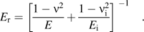 $${E_{\rm{r}}} = {\left[ {{{1 - {\nu ^2}} \over E} + {{1 - \nu _{\rm{i}}^2} \over {{E_{\rm{i}}}}}} \right]^{{\rm{\ }} - 1}}\quad {\rm{.}}$$
Applying the Π theoremReference Brand26 in dimensional analysis, Eq. (4) becomes
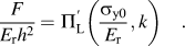 $${F \over {{E_{\rm{r}}}{h^2}}} = \Pi _{\rm{L}}^\prime \left( {{{{\sigma _{{\rm{y}}0}}} \over {{E_{\rm{r}}}}},k} \right)\quad {\rm{.}}$$
For sharp indentation, the load–depth curve during loading follows Kick's law
 $$F = C{h^2}\quad {\rm{,}}$$
where C is the loading curvature. Replacing F/h 2 with C in Eq. (6) leads to
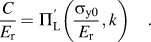 $${C \over {{E_{\rm{r}}}}} = \Pi _{\rm{L}}^\prime \left( {{{{\sigma _{{\rm{y}}0}}} \over {{E_{\rm{r}}}}},k} \right)\quad {\rm{.}}$$
Alternatively, Eq. (8) can be written as
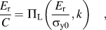 $${{{E_{\rm{r}}}} \over C} = {\Pi _{\rm{L}}}\left( {{{{E_{\rm{r}}}} \over {{\sigma _{{\rm{y}}0}}}},k} \right)\quad {\rm{,}}$$
where ΠL is a dimensionless function. From Eq. (9), it is clear that the loading curvature C is independent of the indentation depth while merely depends on the material properties.
2. Dimensional analysis of unloading
In the unloading segment, besides the eight independent governing parameters appear in loading, the load, F, is related to the initial unloading depth, h m, where the unloading takes place. It is now a function of nine independent governing parameters as given below:
 $$F = {f_{\rm{u}}}\left( {h,{h_{\rm{m}}};E,\nu ,{\sigma _{{\rm{y}}0}},k;{E_{\rm{i}}},{\nu _{\rm{i}}},\alpha } \right)\quad {\rm{.}}$$
Similarly, fixing the included half-angle, α, and combining the elasticity effects of the indenter and sample, Eq. (10) can be rewritten as
 $$F = {f_{\rm{u}}}\left( {h,{h_{\rm{m}}};{E_{\rm{r}}},{\sigma _{{\rm{y}}0}},k} \right)\quad {\rm{.}}$$
Dimensional analysis yields
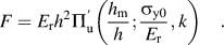 $$F = {E_{\rm{r}}}{h^2}\Pi _{\rm{u}}^\prime \left( {{{{h_{\rm{m}}}} \over h};{{{\sigma _{{\rm{y}}0}}} \over {{E_{\rm{r}}}}},k} \right)\quad {\rm{.}}$$
Taking the derivative with respect to the indentation depth and evaluating it at h m, the initial unloading stiffness, S, is obtained as
 $$S \,\equiv\, {\left. {{{{\mathop{\rm d}\nolimits} F} \over {{\mathop{\rm d}\nolimits} h}}} \right|_{h = {h_{\rm{m}}}}} = {E_{\rm{r}}}{h_{\rm{m}}}\Pi _{\rm{u}}^{\prime \prime }\left( {{{{\sigma _{{\rm{y}}0}}} \over {{E_{\rm{r}}}}},k} \right)\quad {\rm{.}}$$
Alternatively, Eq. (13) can be written as
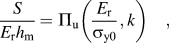 $${S \over {{E_{\rm{r}}}{h_{\rm{m}}}}} = {\Pi _{\rm{u}}}\left( {{{{E_{\rm{r}}}} \over {{\sigma _{{\rm{y}}0}}}},k} \right)\quad {\rm{,}}$$
where Πu is a dimensionless function. It reveals that the initial unloading stiffness, S, is relevant to the elastic–plastic properties of the sample and the initial unloading depth.
B. Finite element analysis
The two dimensionless functions, ΠL [see Eq. (9)] and Πu [see Eq. (14)], relate the elastic–plastic parameters to the load–depth curve parameters. Finite element simulations were implemented in ABAQUS (HKS, Inc., Pawtucket, RI) to illustrate the scaling relationships given by Eqs. (9) and (14).
1. Computational model
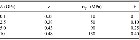
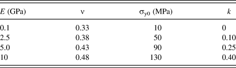
A rigid conical indenter with an included half-angle of 70.3° indenting into an elastic-perfectly plastic sample was considered. An axisymmetric two-dimensional finite element model, which adopts four-node bilinear axisymmetric quadrilateral elements, was constructed to simulate the instrumented sharp indentation. The width of the sample was set to be ten times larger than the radius of the contact region, so that the sample can be regarded as an infinite half-space. The finite element mesh is the same as that used in Ref. Reference Peng, Zhang, Feng and Yang27, which consists of a fine mesh of 2736 elements near the contact region and a gradually coarser mesh of 1031 elements further from the contact region. The contact between the indenter and the sample was modeled as frictionless. The linear Drucker–PragerReference Drucker and Prager7 model and the associated plastic flow rule were used in the plasticity theory. To define an elastic-perfectly plastic material which is sensitive to the hydrostatic pressure, four mechanical parameters (the elastic modulus, E, Poisson's ratio, ν, the yield strength under the pure shear deformation, σy0, and the coefficient of internal friction, k) need to be as input into ABAQUS. Table I lists the parameters used for definition of materials. Each mechanical parameter takes 4 values, and the combination of these parameters leads to 44 = 256 materials. Eliminating the impossible combinations (e.g., E = 0.1 GPa and σy0 = 130 MPa, where the yield strength is greater than the elastic modulus), indentations in 180 combination materials were simulated.
The mechanical parameters input into ABAQUS for defining materials.
2. Computational results
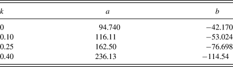
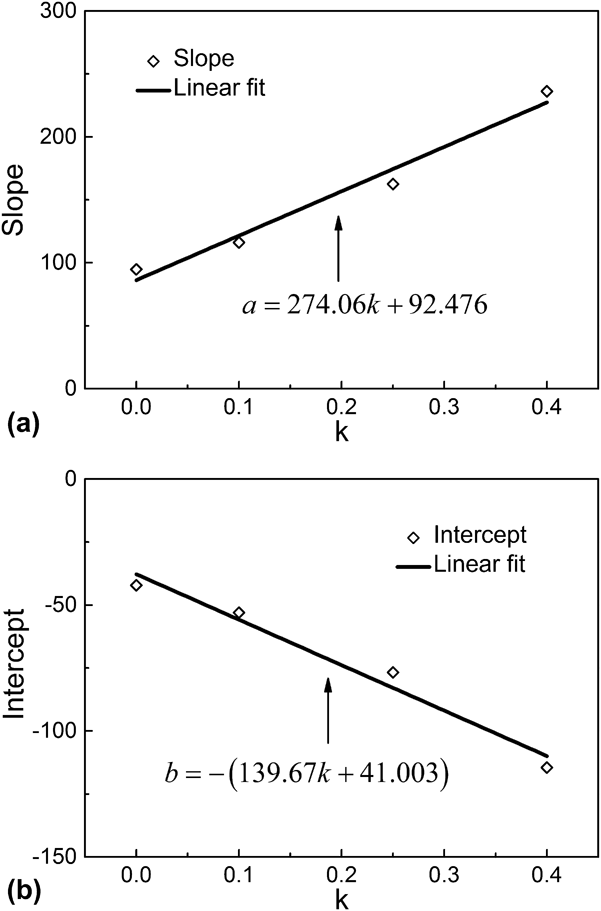
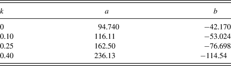
Figure 2 shows the correlations between E r/C and E r/σy0. Clearly, the evolution of the dimensionless function ΠL [see Eq. (9)] is influenced by the coefficient of internal friction, k. For each value of the coefficient of internal friction, a linear relationship exists between E r/C and E r/σy0. Fitting a linear equation, E r/σy0 = a(E r/C) + b, to the data points for each value of k, a set of best-fit slopes and intercepts were obtained (Table II). Plotting the slope versus k and the intercept versus k in Fig. 3, it was found that the slope, a, increases and the intercept, b, decreases generally linearly with k
 $$a = 274.06k + 92.476$$
and
 $$b = - \left( {139.67k + 41.003} \right)\quad {\rm{.}}$$
Correlations between E r/C and E r/σy0. For each value of k, a linear relationship exists between E r/C and E r/σy0. (Solid lines are the best-fitting straight lines to the data points for different k.)
The slopes and intercepts of the fitting lines for different coefficients of internal friction.
Linear dependence of (a) the slope and (b) the intercept of the fitting lines in Fig. 2 on the coefficient of internal friction, k.
Consequently, the scaling relationship between E r/σy0 and E r/C can be described by the following expression:
 $${{{E_{\rm{r}}}} \over {{\sigma _{{\rm{y}}0}}}} = \left( {274.06k + 92.476} \right){{{E_{\rm{r}}}} \over C} - \left( {139.67k + 41.003} \right)\quad {\rm{.}}$$
We plotted S/E rh m versus E r/σy0 in Fig. 4, and the abscissa was scaled logarithmically. It can be found that all data points lie approximately on a single curve, which means that the relationship between S/E rh m and E r/σy0 is insensitive to the coefficient of internal friction. The evolution of the dimensionless function Πu [see Eq. (14)] is relatively easy. Fitting a logarithmic equation,  ${S \mathord{\left/ {\vphantom {S {E_{\rm{r}} h_{\rm{m}} }}} \right. \kern-\nulldelimiterspace} {E_{\rm{r}} h_{\rm{m}} }} = c\ln \left( {{{E_{\rm{r}} } \mathord{\left/ {\vphantom {{E_{\rm{r}} } {\sigma _{{\rm{y}}0} }}} \right. \kern-\nulldelimiterspace} {\sigma _{{\rm{y}}0} }}} \right) + d$, to the data points in Fig. 4, we obtain
 $${S \over {{E_{\rm{r}}}{h_{\rm{m}}}}} = 0.95661\ln \left( {{{{E_{\rm{r}}}} \over {{\sigma _{{\rm{y}}0}}}}} \right) + 1.7181\quad {\rm{.}}$$
Correlations between S/E rh m and E r/σy0. All data points lie approximately on a logarithmic curve. (Solid curve is the best-fitting logarithmic curve to all data points.)
Equations (17) and (18) relate the elastic–plastic properties to the load–depth curve parameters. Rewriting Eqs. (17) and (18) together, we obtain
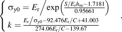 $$\left\{ \matrix{ {\sigma _{{\rm{y}}0}} = {{{E_{\rm{r}}}} \mathord{\left/ {\vphantom {{{E_{\rm{r}}}} {\exp \left( {{{{S \mathord{\left/ {\vphantom {S {{E_{\rm{r}}}{h_{\rm{m}}}}}} \right. \kern-\nulldelimiterspace} {{E_{\rm{r}}}{h_{\rm{m}}}}} - 1.7181} \over {0.95661}}} \right)}}} \right. \kern-\nulldelimiterspace} {\exp \left( {{{{S \mathord{\left/ {\vphantom {S {{E_{\rm{r}}}{h_{\rm{m}}}}}} \right. \kern-\nulldelimiterspace} {{E_{\rm{r}}}{h_{\rm{m}}}}} - 1.7181} \over {0.95661}}} \right)}} \hfill \cr k = {{{{{E_{\rm{r}}}} \mathord{\left/ {\vphantom {{{E_{\rm{r}}}} {{\sigma _{{\rm{y}}0}}}}} \right. \kern-\nulldelimiterspace} {{\sigma _{{\rm{y}}0}}}} - 92.476{{{E_{\rm{r}}}} \mathord{\left/ {\vphantom {{{E_{\rm{r}}}} C}} \right. \kern-\nulldelimiterspace} C} + 41.003} \over {274.06{{{E_{\rm{r}}}} \mathord{\left/ {\vphantom {{{E_{\rm{r}}}} C}} \right. \kern-\nulldelimiterspace} C} - 139.67}} \hfill \cr} \right.\quad {\rm{.}}$$
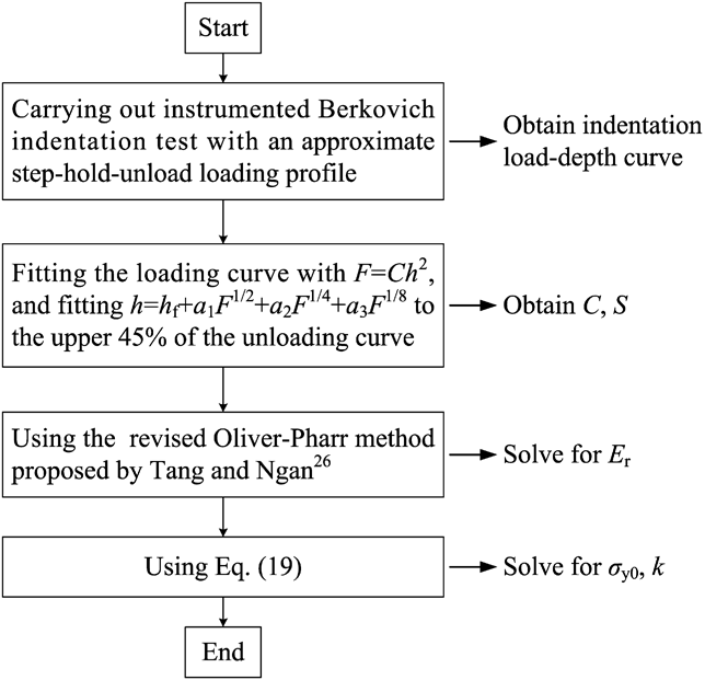
As a direct application of this expression, a method, as illustrated in Flow chart 1, has been developed for evaluating the effect of hydrostatic pressure on the yield strength of solid polymers by instrumented indentation. In Eq. (19), the reduced modulus, E r, can be determined using the revised Oliver–Pharr method proposed by Tang and Ngan,Reference Tang and Ngan28 which adopted the true initial unloading stiffness, S, instead of the apparent initial unloading stiffness, S app, to obtain a more accurate modulus. The true initial unloading stiffness, S, is calculated by
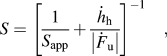 $$S = {\left[ {{1 \over {{S_{{\rm{app}}}}}} + {{{{\dot h}_{\rm{h}}}} \over {\left| {{{\dot F}_{\rm{u}}}} \right|}}} \right]^{ - 1}}\quad {\rm{,}}$$
where the apparent initial unloading stiffness, S app, is obtained by fitting the unloading load–depth curves;  ${\dot h_{\rm{h}}}$ is the creep rate (dh/dt) at the end of holding;
 ${\dot F_{\rm{u}}}$ is the unloading rate (dF/dt) at the beginning of unloading. When the reduced modulus, E r, is determined, the yield strength under the pure shear deformation, σy0, and the coefficient of internal friction, k, can be extracted from indentation load–depth curves.
Load–depth curves obtained from finite element simulation of conical indentations on a pressure-insensitive plastic material and a pressure-sensitive plastic material. The loading curves for these two materials superpose each other, but the unloading curves deviate from each other.
III. DISCUSSION OF UNIQUENESS AND SENSITIVITY
A. Uniqueness of forward and reverse analysis
To discuss the uniqueness of the forward analysis, computational results from the typical elastic–plastic parameters used by Seltzer et al.Reference Seltzer, Cisilino, Frontini and Mai23 were taken as input to predict the load–depth response. Seltzer et al.Reference Seltzer, Cisilino, Frontini and Mai23 simulated a conical indenter with an included half-angle of 70.3° indenting into two materials (a pressure-sensitive material, M 1, with E = 5 GPa, ν = 0.4, σyc = 60 MPa, and k = 0.39, and a pressure-insensitive material, M 2, with E = 5 GPa, ν = 0.4, σyc = 140 MPa, and k = 0) using ABAQUS, where σyc indicates the yield strength in compression. They pointed out that the computational results are nonunique because the indentation tests of these two materials yield the same loading–unloading curve. We repeated Seltzer'sReference Seltzer, Cisilino, Frontini and Mai23 finite element simulations in ABAQUS and found out that their results may not be correct. The computational results are shown in Fig. 5. It is clear that the loading curves for these two materials superpose each other, but the unloading curves deviate from each other.
Load–depth curves obtained from experimental Berkovich indentations of (a) PP, (b) PC, and (c) UPVC. The loading curvature, C, can be obtained by fitting the loading curve with F = Ch 2, and the initial unloading stiffness, S, can be obtained by firstly fitting a polynomial, h = h f + a 1F 1/2 + a 2F 1/4 + a 3F 1/8, to the upper 45% of the unloading curves and then evaluating the derivative with respect to the indentation depth at the initial unloading depth, h m.
A qualitative analysis was used to explain that the indentation tests of two materials with different sets of plastic properties cannot yield the same loading–unloading curve. During loading, the high hydrostatic pressure beneath the conical indenter causes the yield strength of pressure-sensitive materials to increase markedly. When the increased yield strength of a pressure-sensitive material equals the yield strength of a pressure-insensitive material, the indentation tests of these two materials yield the same loading curve if the elastic properties are identical. For example, due to the influence of the high hydrostatic pressure during loading, the yield strength of the pressure-sensitive material, M 1, increases to 140 MPa. In this case, M 1 and M 2 have the same elastic modulus, Poisson's ratio, and apparent yield strength. The indentation tests of these two materials yield the same loading curve. During unloading, however, the hydrostatic pressure beneath the indenter decreases dramatically. The hydrostatic pressure is much smaller than that during loading. This means that the increased yield strength of the pressure-sensitive material, M 1, during unloading is no longer equal to 140 MPa. Thus, the unloading curves for materials, M 1 and M 2, will deviate from each other. To sum up, the increment of the yield strength of a pressure-sensitive material during loading is different from that during unloading because the hydrostatic pressures beneath the indenter are different during loading and unloading. For a pressure-sensitive material, the apparent elastic–plastic properties are different during loading and unloading. Even if the apparent elastic–plastic properties of a pressure-sensitive material are identical to those of a pressure-insensitive material during loading, the apparent elastic–plastic properties will be different during unloading. As a consequence, the loading curves and the unloading curves for a pressure-sensitive material and a pressure-insensitive material cannot coincide with each other simultaneously. This indicates that the loading–unloading curves for materials with different sets of plastic properties are unique.
For the reverse analysis, E r can be uniquely determined from a single load–depth curve using the revised Oliver–Pharr method presented by Tang and Ngan.Reference Tang and Ngan28 To verify the uniqueness of the reverse analysis for evaluating σy0 and k, a simple and practical method proposed by Cheng and ChengReference Cheng and Cheng29 was adopted. Drawing a straight line in Fig. 2 parallel to the horizontal axis (i.e., the E r/σy0 axis). The values of σy0 and k corresponding to the intersections of the horizontal line and E r/C lead to the same loading curves. It is evident that several sets of σy0 and k will yield the same loading curve. Similarly, drawing a straight line in Fig. 4 parallel to the E r/σy0 axis. As all data points lie approximately on a monotone increasing curve, there is only one intersection. This means that the yield strength under the pure shear deformation, σy0, can be uniquely extracted from the unloading curve using Eq. (18). When σy0 was determined, the coefficient of internal friction, k, was then uniquely evaluated from the loading curve by Eq. (17).
B. Sensitivity to the loading curvature and initial unloading stiffness
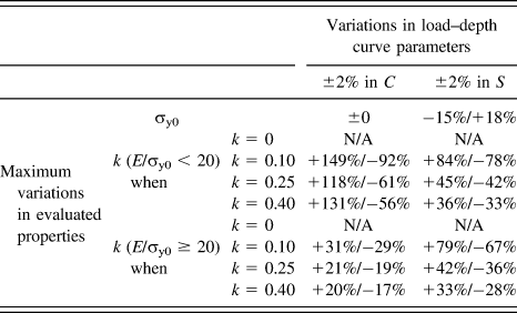
As the accuracy of the mechanical properties of the indented materials evaluated through reverse analysis depends on the accuracy with which the load–depth responses are measured, the sensitivity of the evaluated mechanical properties to the variations in the parameters obtained from the load–depth curves was investigated by using the computational indentation data of the 180 combination materials obtained in Sec. II. B. For each combination material, the sensitivity of the evaluated plastic properties to variations in load–depth curve parameters, C and S, about the reference values that obtained from the computational data was examined. The maximum variations are summarized in Table III for conservative estimation.
Sensitivity to the loading curvature and initial unloading stiffness.
It is clear that σy0 is insensitive to the loading curvature, C, and has moderate sensitivity to the initial unloading stiffness, S; for high elasticity materials (E/σy0 < 20), k displays strong sensitivity to C and S; for lower elasticity materials (E/σy0 ≥ 20), k displays strong sensitivity to C and S when k < 0.25, and displays moderate sensitivity with respect to C and strong sensitivity to S when k ≥ 0.25. It can also be found out from Table III that the sensitivity of k to C and S decreases with the increase of k. One of the reasons for the strong sensitivity of k to the variations in C and S may be that the value of k is small as a denominator. For example, the absolute deviation of k is 0.05, the relative deviation is 10% if the reference value of k is 0.5, while the relative deviation will be 100% for a reference value of 0.05. Though the relative deviations of k seem to be large when there is a variation of ±2% in C or S, the maximum absolute deviation of k is about ±0.12 and most of the absolute deviations of k are within the range from −0.07 to 0.07 for lower elasticity materials (E/σy0 ≥ 20).
IV. EXPERIMENTS
PP, PC, and UPVC (Anheda Plastic Products Co., Ltd., Suzhou, China) were used for experimental materials. For instrumented indentation tests, the 4.0-mm-thick PP, PC, and UPVC plates were cut into small squares measuring 20 mm × 20 mm. All specimens were annealed (at 100 °C for PP, at 150 °C for PC, and at 102 °C for UPVC) for 2.5 h in air to relieve the residual stress caused by mechanical processing.
A MTS Nano Indenter XP system (MTS Nano Instruments, Oak Ridge, TN) was used to carry out the instrumented indentation tests. The indenter used in the tests is a Berkovich indenter, which can be modeled equivalently as a cone with an included half-angle of 70.3°. An air-conditioner was used to adjust the room temperature to guarantee that the indentation tests were performed around 23 °C. According to the method proposed in this work, an approximate step-hold-unload loading profile was adopted. The load was increased quickly to the maximum (12.5 mN) in 2 s, held at the maximum load for 300 s and finally decreased linearly to zero in 50 s. For each material, the indentation tests were repeated 5 times. During the tests, the thermal drift rate was within ±0.02 nm/s. The possible maximum thermal drift was ±7 nm for a test that lasts 350 s, which is much smaller than the indentation depth (about 2 μm).
V. RESULTS
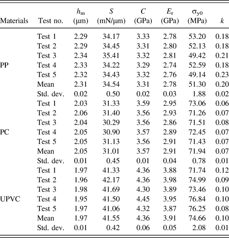
Table IV lists the values of the measurement parameters (h m, S, and C) that need to be known to determine the elastic–plastic parameters. They were obtained directly or indirectly from the indentation load–depth curves. The true initial unloading stiffness, S, was calculated by Eq. (20). The apparent initial unloading stiffness, S app, was obtained by firstly fitting a polynomial, h = h f + a 1F 1/2 + a 2F 1/4 + a 3F 1/8, to the upper 45% of the unloading curves (see Fig. 6) and then evaluating the derivative with respect to the indentation depth at h m. The reason for using the polynomial of “h = h f + a 1F 1/2 + a 2F 1/4 + a 3F 1/8” is that it can fit the unloading load–depth curves better than the Oliver–Pharr formula, F = a(h + h f)m, does for polymers.Reference Tang and Ngan28 Fitting the loading curve with F = Ch 2, the loading curvature, C, was obtained. Because the indenter tip roundness and the surface roughness of sample may influence the load–depth curve when the indentation is shallow, we did not fit the loading curve where the depth is less than 300 nm (see Fig. 6). The reduced modulus, E r, was determined using the revised Oliver–Pharr method proposed by Tang and Ngan.Reference Tang and Ngan28
The measurement parameters and the elastic–plastic parameters obtained by instrumented Berkovich indentation.
Reverse analysis algorithm for evaluating the effect of the hydrostatic pressure on the yield strength of solid polymers.
Using the method proposed by Peng et al.,Reference Peng, Zhang, Feng and Huan30 the dominant retardation times obtained are about 14 s for PP, PC, and UPVC. The ratio of the loading time (2 s) to the dominant retardation time is about 1/7 which is very close to Oyen'sReference Oyen24 critical value (1/10). Thus, the viscous effects can be neglected during the fast loading segment. The values of creep factor calculated using Eq. (2) are 3.5% for PP, 1.0% for PC, and 1.9% for UPVC, which are all less than 10%. This demonstrates that the holding is long enough for ignoring the viscous effects during unloading, and the experiments were legitimately carried out. Substituting the values of E r, h m, S, and C into Eq. (19), the yield strength under the pure shear deformation, σy0, and the coefficient of internal friction, k, were calculated. As listed in Table IV, the values of k are 0.20 ± 0.02 for PP, 0.07 ± 0.01 for PC, and 0.10 ± 0.01 for UPVC, which are in good agreement with the values reported in the literature (the mean values are 0.21 for PP,Reference Mears, Pae and Sauer1,Reference Pae31 0.08 for PC,Reference Quinson, Perez, Rink and Pavan6,Reference Sauer, Mears and Pae8,Reference Christiansen, Baer and Radcliffe9 and 0.14 for UPVCReference Pae and Bhateja3).
VI. SUMMARY AND CONCLUSIONS
Using dimensional analysis and with the help of finite element simulations, two analytical expressions [Eqs. (17) and (18)] were derived to relate the indentation data to the plastic properties of solid polymers. These two expressions were used to extract the yield strength under the pure shear deformation, σy0, and the coefficient of internal friction, k, from indentation load–depth curves. The calculated values of k are 0.20 ± 0.02 for PP, 0.07 ± 0.01 for PC, and 0.10 ± 0.01 for UPVC, which agree well with the values reported in the literature. This demonstrates that the instrumented indentation method proposed in the present work is useful to evaluate the effect of hydrostatic pressure on the yield strength of solid polymers.
ACKNOWLEDGMENTS
The authors would like to thank Dr. Y. Huan for specimen processing. The support from the National Natural Science Foundation of China (Grant Nos. 11025212, 11272318, 11402233, and 11302231) and the Young Scholars of Zhejiang Province (R1111149) is gratefully acknowledged.