1 Introduction
Quantitative recurrence has recently been a popular topic in dynamical systems and ergodic theory, since the first results obtained by [Reference Doeblin8] for the Gauss map and by [Reference Pitskel18] for the case of Markov chains. These properties are set by estimating the first return time of a dynamical system into a small neighborhood of its starting point. For further references, see [Reference Saussol22] where some recurrence results in the context of probability-preserving dynamical systems are presented; see also [Reference Abadi and Galves1] for more in this area, and [Reference Saussol21, Reference Saussol22] on rapidly mixing systems. Few results have been established in the case where the dynamical system preserves an infinite measure, but see [Reference Bressaud and Zweimüller6], where Bressaud and Zweimüller have established first results in the case of piecewise affine maps of the interval with infinite measure. The recurrence of
 $\mathbb {Z}$
-extension of subshifts of finite type is investigated in [Reference Yassine23], and the
 $\mathbb {Z}^2$
case is addressed in [Reference Pène and Saussol12], while in [Reference Pène and Saussol14] quantitative recurrence results for T,
 $T^{-1}$
transformations are proved. Other relevant contributions can be found in [Reference Pène and Saussol13, Reference Pène, Saussol and Zweimüller15, Reference Pène, Saussol and Zweimüller16].
In this paper we extend the study to include dynamical systems in continuous time, in the case where the measure is infinite. More precisely, we consider the
 $\mathbb {Z}$
-extension of Axiom A flows, including the geodesic flows on
 $\mathbb {Z}$
-periodic negatively curved manifolds.
Thus, we consider a Riemannian manifold
 $\tilde {M}$
of dimension 3, given by a
 $\mathbb {Z}$
-extension, endowed with a
 $\sigma $
-finite measure
 $\tilde {\mu }$
, and a flow
 $(\tilde {g}_{t})_{t\in \mathbb {R}}$
on
 $\tilde {M}$
that preserves the measure
 $\tilde {\mu }$
. We denote by
 $\Gamma $
an infinite group of isometries of
 $\tilde {M}$
that also preserves the measure
 $\tilde {\mu }$
. We then suppose that
 $M=\tilde {M}/\Gamma $
is a compact manifold, and we define the quotient flow
 $(g_{t})_{t\in \mathbb {R}}$
on M. We define a measure
 $\mu $
on M that is obtained from the measure
 $\tilde {\mu }$
by passing through the quotient. We further assume that
 $\mu $
is an equilibrium measure for the flow
 $g_{t}$
on M, and that
 $(M, (g_{t})_{t})$
is an Axiom A flow.
We are interested in the first return time
 $\tau _{\epsilon }(x)$
of the flow
 $\tilde {g}_{t}$
to an
 $\epsilon $
-neighborhood of its starting point x, defined by
 $$ \begin{align*} \tau_{\epsilon}(x):=\inf\ \{t>1: \tilde{g}_{t}(x)\in B(x,\epsilon)\}, \end{align*} $$
where
 $B(x,\epsilon )$
is the ball of center x and radius
 $\epsilon $
. Studying the asymptotic behavior of
 $\tau _{\epsilon }$
as
 $\epsilon \rightarrow 0$
, we first prove in Theorem 3.1 the following almost everywhere convergence result:
 $$ \begin{align*} \underset{\epsilon\rightarrow0}{\lim}\frac{\log\sqrt{\tau_{\epsilon}}}{-\log\epsilon}=\dim_{\mathrm{H}} \mu -1, \end{align*} $$
where
 $\dim _{\mathrm {H}} \mu $
is the Hausdorff dimension of the measure
 $\mu $
. Moreover, the following convergence holds in distribution, with respect to any probability measure absolutely continuous with respect to
 $\tilde {\mu }$
:
 $$ \begin{align*} \tilde{\nu}_{0}(B(\cdot,\epsilon))\sqrt{\tau_{\epsilon}(\cdot)}\underset{\epsilon\rightarrow0}{\longrightarrow} \sigma_{\mathrm{flow}}\frac{\mathcal{E}}{|\mathcal{N}|}, \end{align*} $$
where
 $\tilde {\nu }_{0}$
is a sectional measure (defined in (3.1)),
 $\sigma ^2_{\mathrm {flow}}$
is an asymptotic variance related to the flow, and
 $\mathcal {E}$
and
 $\mathcal {N}$
are independent random variables,
 $\mathcal {E}$
having an exponential distribution with mean 1 and
 $\mathcal {N}$
having a standard Gaussian distribution (the statement of this result is given in Theorem 3.2).
Moreover, we apply our result in the case of the unit geodesic flow on a
 $\mathbb {Z}$
-cover of a
 $C^2$
compact surface
 $\mathcal {S}$
of negative curvature. The following convergence in distribution holds with respect to any probability measure absolutely continuous with respect to
 $\tilde {\mu }$
:
 $$ \begin{align*} \frac{\epsilon^2}{2 \mathrm{Vol}( \mathcal{S})}\sqrt{\tau_{\epsilon}(\cdot)}\underset{\epsilon\rightarrow0}{\longrightarrow} \sigma_{\mathrm{flow}}\frac{\mathcal{E}}{|\mathcal{N}|}. \end{align*} $$
where
 $\mathcal {E}$
and
 $\mathcal {N}$
are two independent random variables as above (see Theorem 6.1 for the precise statement).
In this paper, we start by introducing in §2 all the necessary notions and results from hyperbolic dynamics concerning Axiom A flows and a hyperbolic set for a flow. In particular, we consider the Markov section constructed by Bowen [Reference Bowen5] and Ratner [Reference Ratner19] for a locally maximal hyperbolic set. We note that any smooth flow with a hyperbolic set can be represented as a suspension flow over a mixing subshift of finite type. Another point is to describe how a Markov section for a hyperbolic set gives rise to a symbolic dynamics (see §2.1). We consider a set
 $\Sigma _{A}$
together with the shift map
 $\sigma $
. Then we give a definition of the coding map
 $\chi :\Sigma _{A}\rightarrow X$
. Thus, in the same way we define the symbolic suspension flow
 $\mathbf {S}=\{\mathbf {S}_{t}\}_{t\in \mathbb {R}}$
over
 $\sigma _{|\Sigma _{A}}$
. We establish some properties on balls and coding. We introduce in §3 the model of
 $\mathbb {Z}$
-extension we are interested in. We show that a given ball contains and is contained in a suitable cylinder. This serves in studying the asymptotic behavior of our return time to a cylinder and then inferring the return time to a ball, and yet establishing the desired almost sure convergence (in §4) and convergence in distribution results (in §5). Finally, we apply our results to prove the convergence in distribution theorem in the case where the flow is a geodesic flow on a
 $\mathbb {Z}$
-periodic negatively curved manifold (in §6).
2 Definition and properties of Axiom A flows
Let M be a Riemannian smooth manifold of dimension 3. We consider a
 $C^{1}$
flow
 $(g_{t})_{t\in \mathbb {R}}$
on M. A compact
 $g_{t}$
-invariant set
 $\Lambda \subset M$
is said to be a hyperbolic set for
 $g_{t}$
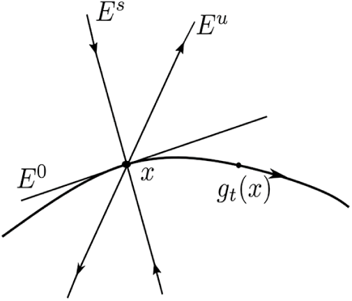
if there exists a continuous splitting of the tangent space,
 $T_{\Lambda }M= E^{s}\oplus E^{u}\oplus E^{0}$
(see Figure 1), and constants
 $c>0$
and
 $\unicode{x3bb} \in (0,1)$
such that for each
 $x\in \Lambda $
and
 $t\in \mathbb {R}$
:
-
(1) the vector
 ${d g_{t}(x)}/{dt}{\mid} _{t=0}$
generates
$E^{0}(x)$
, which is the flow direction;
-
(2)
$d_{x}g_{t}E^{s}(x)=E^{s}(g_{t}(x))$
and
$d_{x}g_{t}E^{u}(x)=E^{u}(g_{t}(x))$
; -
(3) for all
$t>0$
,
$\|d_{x}g_{t}v\|\leq c\unicode{x3bb} ^{t}\|v\| \text { for } v\in E^{s}(x)$
, and
$ \|d_{x}g_{-t}v\|\leq c\unicode{x3bb} ^{t}\|v\| $
for
${v\in E^{u}(x).}$


The subspaces
 $E^{s}(x)$
and
 $E^{u}(x)$
are called the stable and unstable subspaces at x; they depend continuously on the point and are invariant. For each
 $x\in \Lambda $
, there exist stable and unstable local manifolds at the point x,
 $W^{s}_{\mathrm {loc}}(x)$
and
 $W^{u}_{\mathrm {loc}}(x)$
, which are tangent to the contracting and expanding subspaces and contain the point x:
-
(1)
$x\in W^{s}_{\mathrm {loc}}(x) $
and
$x\in W^{u}_{\mathrm {loc}}(x) $
; -
(2)
$T_{x}W^{s}_{\mathrm {loc}}(x)=E^{s}(x)$
and
$T_{x}W^{u}_{\mathrm {loc}}(x)=E^{u}(x)$
; -
(3) for each
$t>0$
,
$g_{t}(W^{s}_{\mathrm {loc}}(x))\subset W^{s}_{\mathrm {loc}}(g_{t}(x))$
,
$g_{-t}(W^{u}_{\mathrm {loc}}(x))\subset W^{u}_{\mathrm {loc}}(g_{-t}(x))$
; -
(4) there exist
$\kappa>0$
and
$\vartheta>0$
such that for each
$t>0$
, we have (2.1)and
$$ \begin{align} d(g_{t}(x), g_{t}(y))\leq \kappa e^{-\vartheta t}d(x,y) \quad \text{for } y\in W^{s}_{\mathrm{loc}}(x), \end{align} $$
$$ \begin{align*} d(g_{-t}(x), g_{-t}(y))\leq \kappa e^{-\vartheta t}d(x,y) \quad \text{for } y\in W^{u}_{\mathrm{loc}}(x), \end{align*} $$


where d is the distance induced in M by the Riemannian metric. A hyperbolic set
 $\Lambda $
is said to be locally maximal (with respect to a flow
 $g_{t}$
) if there exists an open neighborhood U of
 $\Lambda $
such that
 $$ \begin{align*} \Lambda=\bigcap_{t\in\mathbb{R}}g_{t}(U). \end{align*} $$
Let
 $\Lambda $
be a locally maximal hyperbolic set. For every
 $\epsilon>0$
there is
 $\delta>0$
such that for any
 $x,y$
in
 $\Lambda $
with
 $d(x,y)\leq \delta $
there exists a unique
 $t=t(x,y)\in [-\epsilon ,\epsilon ]$
, for which the intersection
 $$ \begin{align*} [x,y]:= W^{s}_{\mathrm{loc}}(g_{t}(x))\cap W^{u}_{\mathrm{loc}}(y) \end{align*} $$
consists of a single point in
 $\Lambda $
; moreover, the map
 $(x,y)\mapsto t(x,y)$
is continuous.
The splitting of a hyperbolic set.

We define the global stable and unstable manifolds at a point
 $x\in \Lambda $
by
 $$ \begin{align*}W^{s}(x)=\bigcup_{t\geq 0}g_{-t}(W^{s}_{\mathrm{loc}}(g_{t}(x))), \quad W^{u}(x)=\bigcup_{t\geq 0}g_{t}(W^{u}_{\mathrm{loc}}(g_{-t}(x))).\end{align*} $$
They can be characterized as follows:
 $$ \begin{align*} W^{s}(x)&=\{y\in \Lambda: d(g_{t}(x), g_{t}(y))\rightarrow0 \text{ as } t\rightarrow\infty\},\\W^{u}(x)&=\{y\in \Lambda: d(g_{-t}(x), g_{-t}(y))\rightarrow0 \text{ as } t\rightarrow\infty\}. \end{align*} $$
A flow
 $(g_{t})_{t\in \mathbb {R}}$
is said to be an Axiom A flow if its set of non-wandering points is hyperbolic: a point
 $x \in M$
is called a non-wandering point if for every open neighborhood
 $\mathcal {O}$
of x there is a time
 $t_{x}> 0$
such that
 $g_{t_{x}}(\mathcal {O})\cap \mathcal {O}\neq \emptyset $
. Throughout this paper, we consider
 $(g_{t})_{t\in \mathbb {R}}$
an Axiom A flow and topologically mixing on a locally maximal hyperbolic set
 $\Lambda $
. A decomposition of this set provides an analysis of its dynamics, the construction of the Markov collection, which was developed by Bowen [Reference Bowen5] and Ratner [Reference Ratner19]. Given a point
 $x\in \Lambda $
, consider a small compact disk
 $D\subset M$
containing x of codimension
 $1$
which is transversal to the flow
 $g_{t}$
. This disk is a local section of the flow, that is, there exists
 $\tau>0$
such that the map
 $(x,t)\rightarrow g_{t}(x)$
is a diffeomorphism of the direct product
 $D\times [-\tau ,\tau ]$
onto a neighborhood
 $U_{\tau }(D)$
:
 $$ \begin{align*} \varphi_{D}: D\times [0,\tau]&\rightarrow U_{\tau}(D):= \varphi_{D}(D\times[0,\tau])\subset M,\\(x,t)&\rightarrow y= g_{t}(x). \end{align*} $$
The function
 $\varphi _{D}$
is Lipschitz. We set
 $k_{\varphi _{D}}:=\max _D({\mathrm {Lip}}\ \varphi _{D}, {\mathrm {Lip}}\ \varphi _{D}^{-1})$
.
The projection
 $P_{D}: U_{\tau }(D)\rightarrow D$
, defined such that
 $ P_{D}(z):=g_{-s}(z)$
, where
 $s>0$
is the minimum value by
 $g_{t}(z)\in D$
, is a differentiable map. Consider now a closed set
 ${\Pi \subset \Lambda \cap D}$
which does not intersect the boundary
 $\partial D$
. For any two points y,
 $z\in \Pi $
, we set
 $$ \begin{align} \{y,z\}:=P_{D}([y,z]). \end{align} $$
The set
 $\Pi $
is said to be a rectangle if
 $\Pi =\overline {\text {int}\ \Pi }$
(where the interior is considered with respect to the induced topology of
 $\Lambda \cap D$
) and
 $\{y,z\}\in \Pi $
for any
 $y,z\in \Pi $
.
Since we are working on a three-dimensional manifold, the flow
 $(g_t)_t$
is conformal. We have the following proposition:
Proposition 2.1. [Reference Barreira3, Reference Hasselblatt10]
Let
 $\Pi $
be a rectangle. The maps
 $x\mapsto E^{s}(x)\oplus E^{0}(x)$
and
 ${x\mapsto E^{u}(x)\oplus E^{0}(x)}$
are Lipschitz. This implies that there exists
 $c_{\mathrm {L}}>0$
such that
 ${\Pi \times \Pi \ni (x,y)\mapsto \{x,y\}\in \Pi }$
is a Lipschitz map of Lipschitz constant
 $c_{\mathrm {L}}>0$
and that
 $\{x,\cdot\}$
and
 $\{\cdot,y\}$
have uniformly Lipschitz inverses.
Let
 $\Pi $
be a rectangle, then for every
 $x\in \Pi $
, we set
 $$ \begin{align*} W^{s}_{\mathrm{loc}}(x,\Pi)&=\{\{x,y\}:y\in\Pi\}=\Pi\cap P_{D}(U_{\tau}(D)\cap W^{s}_{\mathrm{loc}}(x)), \\W^{u}_{\mathrm{loc}}(x,\Pi)&=\{\{x,y\}:y\in\Pi\}=\Pi\cap P_{D}(U_{\tau}(D)\cap W^{u}_{\mathrm{loc}}(x)). \end{align*} $$
We now consider a collection of rectangles
 $\Pi _{1},\ldots ,\Pi _{n}$
(each contained in some open disk transversal to the flow) such that
 $\Pi _{i}\cap \Pi _{j}=\partial \Pi _{i}\cap \partial \Pi _{j} \mbox { for } i\neq j.$
Set
 $X=\bigcup _{i=1}^{n}\Pi _{i}$
. We assume that there exists
 $\beta _{0}>0$
such that:
-
(1)
$\Lambda =\bigcup _{t\in [0,\beta _{0}]}g_{t}(X)$
; -
(2) for each
$i\neq j$
, for every
$t\in [0,\beta _{0}]$
, at least
$g_{t}(\Pi _{i})\cap \Pi _{j}=\emptyset \mbox { or }g_{t}(\Pi _{j})\cap \Pi _{i}=\emptyset $
.


The set X is a Poincaré section for the flow
 $g_{t}$
. The height function R is defined such that for every
 $ x\in X$
, one can find the smallest positive number
 $R(x)$
such that
 $g_{R(x)}(x)\in X$
. The Poincaré map
 $T:X\longrightarrow X$
is defined by
 $T(x)= g_{R(x)}(x)$
. A Markov collection is a finite collection of rectangles
 $\Pi _{1},\ldots ,\Pi _{n}$
satisfying, for every
 $x\in \text {int}\ \Pi _{i}\cap \text {int}\ T^{-1}(\Pi _{j})$
,
 $$ \begin{align*} T(\text{int}\ (W_{\mathrm{loc}}^{s}(x)\cap \Pi_{i}))\subset\text{int}\ (W_{\mathrm{loc}}^{s}(T(x))\cap \Pi_{j}), \end{align*} $$
and for every
 $x\in \text {int}\ \Pi _{i}\cap \text {int}\ T(\Pi _{k})$
,
 $$ \begin{align*} T^{-1}(\text{int}\ (W_{\mathrm{loc}}^{u}(x)\cap \Pi_{i}))\subset\text{int}\ ( W_{\mathrm{loc}}^{u}(T^{-1}(x))\cap \Pi_{k}). \end{align*} $$
It follows from the work of Bowen [Reference Bowen5] and Ratner [Reference Ratner19] that any locally maximal hyperbolic set
 $\Lambda $
has a Markov collection of arbitrary small diameter. Given a rectangle
 $\Pi _{i}$
, we call the set
 $$ \begin{align} R_{i}=\bigcup_{x\in \Pi_{i}}\bigcup_{0\leq t\leq R(x)}g_{t}(x)\subset \Lambda \end{align} $$
a Markov set. Note that
 $R_{i}=\overline {\text {int}\ R_{i}}$
and
 $\text {int}\ R_{i}\cap \text {int}\ R_{j}=\emptyset $
for
 $i\neq j$
.
2.1 Suspension flow
 $T:X\rightarrow X$
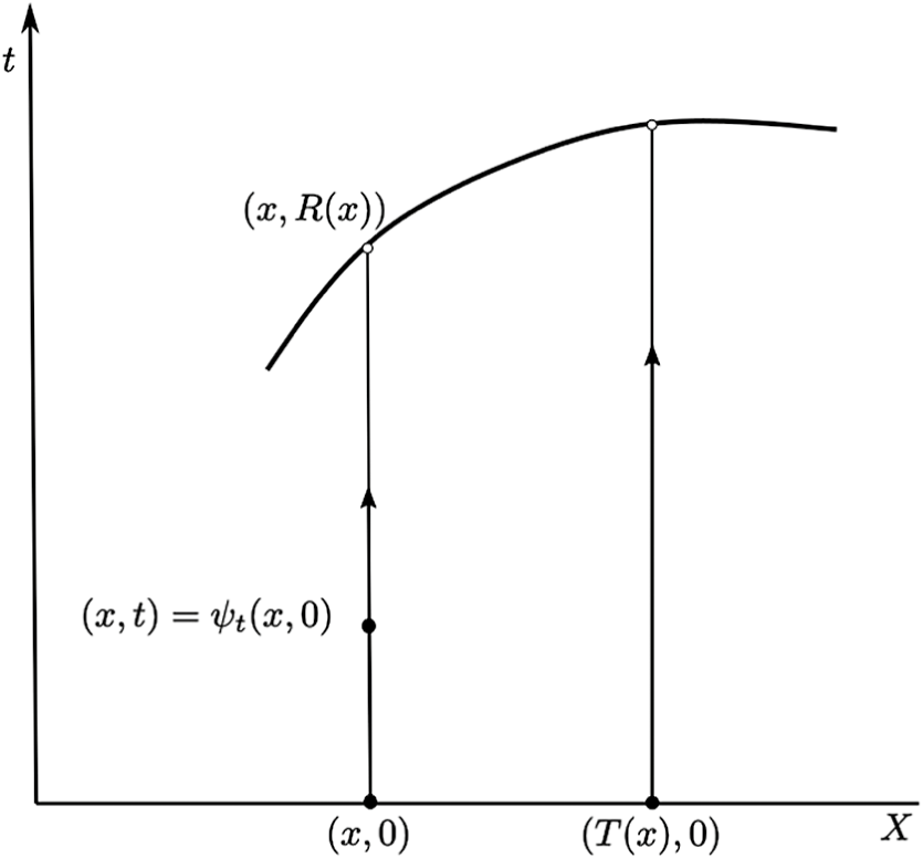
being the Poincaré map restricted on X, and R the height function, we consider the space
 $ X_{R}=\{(x,s)\in X\times \mathbb {R} \text { : } 0\leq s\leq R(x) \},$
where the points
 $(x,R(x))$
and
 $(T(x), 0)$
are identified for each
 $x\in X$
. The suspension flow over T, with height function R, is the flow
 $\psi =\{\psi _{t}\}_{t\in \mathbb {R}}$
in
 $X_{R}$
, given by
 $$ \begin{align} \psi_{t}(x,s)=(T^{n}x, s+t-S_{n}R(x)), \end{align} $$
(see Figure 2) where n is the unique non-negative integer such that
 $0\leq s+t-S_{n}R(x)<R(T^{n}x)$
, that is,
 $$ \begin{align*} S_{n}R(x)\leq s+t<S_{n+1}R(x), \end{align*} $$
where we set as usual
 $S_{n}R=\sum _{k=0}^{n-1}R\circ T^{k}$
.
A suspension flow
 $\psi=\{\psi_{t}\}_{t\in\mathbb{R}}$
over T.

Using a Markov collection of a hyperbolic set
 $\Lambda $
, we can obtain a symbolic representation of the flow
 $g_{t}$
. Let
 $\Lambda $
be a locally maximal hyperbolic set for the flow
 $g_{t}$
, and given
 $\Pi _{1},\ldots ,\Pi _{n}$
the associated Markov collection. Consider the
 $n\times n$
matrix A with entries
 $$ \begin{align*} a_{ij}= \begin{cases} 1 & \text{if } \text{int }T(\Pi_{i})\cap \text{int }\Pi_{j}\neq\emptyset,\\ 0 & \text{otherwise,} \end{cases} \end{align*} $$
where T is the Poincaré map. We also consider the set
 $\Sigma _{A}$
given by
 $$ \begin{align*} \Sigma_{A}=\{\omega=(\omega_{n})_{n\in \mathbb{Z}}:\text{ for all } n\in \mathbb{Z}, a_{\omega_{n}\omega_{n+1}}=1\}, \end{align*} $$
together with the shift map
 $\sigma :\Sigma _{A}\rightarrow \Sigma _{A} $
defined by
 $\sigma ((\omega _{n})_{n\in \mathbb {Z}})=(\omega _{n+1})_{n\in \mathbb {Z}}$
. Since the flow is topologically mixing, the matrix A is primitive aperiodic, that is, there exists
 $n_{0}\in \mathbb {N}$
such that
 $A^{n_{0}}>0$
. We endow
 $\Sigma _{A}$
with the metric
 $\hat {d}$
given by
 $$ \begin{align*}\hat{d}(\omega, \omega'):=e^{-m},\end{align*} $$
where m is the greatest integer such that
 $\omega _{i}=\omega _{i}'$
whenever
 $|i| < m.$
Let
 $q,q'$
be two positive integers, and
 $a:=a_{-q},\ldots , a_{0},\ldots ,a_{q'}$
be a finite symbol sequence. We define a
 $(-q,q')$
-cylinder by
 $$ \begin{align*}C_{-q,q'}(a)=\{(\omega_{n})_{n\in\mathbb{Z}}\in \Sigma_{A}: \omega_{-q}=a_{-q},\ldots,\omega_{q'}=a_{q'}\}.\end{align*} $$
We denote by
 $C_{-q,q'}(\omega )$
the
 $(-q,q')$
-cylinder containing a point
 $\omega \in \Sigma _{A}$
.
Proposition 2.2. Let
 $\tilde {h}:\Sigma \rightarrow \mathbb {R}$
be a Hölder continuous function. An invariant measure
 $\nu $
is called a Gibbs measure for the potential
 $\tilde {h}$
, if there exists a constant
 ${P_{\sigma }(\tilde {h})\in \mathbb {R}}$
, called the pressure, such that for some
 $k_{\tilde {h}}\geq 1$
, for any
 $\omega $
and any
 $q,q'\geq 0$
,
 $$ \begin{align} \frac{1}{k_{\tilde{h}}}\leq\frac{\nu(C_{-q,q'}(\omega))}{\exp(\sum_{k=-q}^{q'}\tilde{h} (\sigma^{k}(\omega))-(q+q'+1)P_{\sigma}(\tilde{h}))}\leq k_{\tilde{h}}. \end{align} $$
In what follows, let
 $\nu $
be the Gibbs measure on
 $\Sigma _{A}$
associated to some Hölder continuous potential
 $\tilde {h}$
.
Definition 2.3. We consider the coding map
 $\chi :\Sigma _{A}\rightarrow X$
, defined by
 $$ \begin{align*}\chi(\omega)=\underset{n}{\bigcap}\overline{\underset{|k|\leq n}{\bigcap}T^{-k}(\text{int}\ \Pi_{\omega_{k}})}.\end{align*} $$
One can easily verify that the diagram

is commutative, that is,
 $$ \begin{align} \chi\circ\sigma=T\circ\chi, \end{align} $$
and we have
 $\chi _{*}\nu =\nu _{X}$
the measure on X.
As at the beginning of this section, we define in the same way the suspension flow
 $\mathbf {S}=\{\mathbf {S}_{t}\}_{t\in \mathbb {R}}$
over
 $\sigma |_{\Sigma _{A}}$
with the Hölder height function
 $r=R\circ \chi $
. We extend
 $\chi $
to the finite-to-one onto map
 $\chi :\Delta \rightarrow \Lambda $
by
 $\chi (\omega ,s)=(g_{s}\circ \chi )(\omega )$
, for
 $(\omega ,s)\in \Delta $
, where
 ${\Delta :=\{(\omega ,s)\in \Sigma _{A}\times \mathbb {R} \text { : } 0\leq s\leq r(\omega ) \}}$
, with
 $r(\omega )=R(\chi (\omega ))$
. BY (2.6), for every
 $t\in \mathbb {R}$
the diagram

commutes, expressing that the flows
 $g_{t}$
and
 $\mathbf {S}_{t}$
are conjugated, that is,
 $\chi \circ \mathbf {S}_{t}=g_{t}\circ \chi $
. The measure
 $\mu _{\Delta }={(\nu \times {\mathrm {Leb}}|\Delta )}/{(\int _{\Sigma _{A}}r d\nu )}$
is a probability measure on
 $\Delta $
, which is invariant by
 $\mathbf {S}_{t}$
, where
 ${\mathrm {Leb}}$
is the Lebesgue measure on
 $\mathbb {R}$
. And we have
 $\chi _{*}\mu _{\Delta }=\mu $
, where we recall that
 $\mu $
is an equilibrium measure for the flow
 $g_{t}$
.
Let
 $h_\nu (\sigma )$
be the entropy of the invariant measure
 $\nu $
on the system
 $(\Sigma _A, \sigma )$
. For flows, the entropy is defined as the entropy of the time-1 map. We recall Abramov’s formula (see [Reference Abramov2]) which establishes a relation between the entropy of the suspension flow
 $\mathbf {S}_{t}$
and
 $h_\nu (\sigma )$
as follows:
 $$ \begin{align} h_{\mu_{\Delta}}(\mathbf{S}_{t}):= h_{\mu_{\Delta}}(\mathbf{S}_{1})=\dfrac{h_{\nu}(\sigma)}{\int_{\Sigma_A}r d\nu}. \end{align} $$
Moreover, since the systems
 $(\Lambda , g_t,\mu )$
and
 $(\Delta ,\mathbf {S}_t,\mu _\Delta )$
are conjugated, they have the same entropy, thus
 $h_{\mu _{\Delta }}(\mathbf {S}_t)=h_{\mu }(g_t)$
. For the same reason,
 $h_{\nu }(\sigma )=h_{\nu _X}(T)$
. So we have the relation
 $$ \begin{align} h_\mu(g_t)=\frac{h_{\nu_X}(T)}{\int_{X}R \,d\nu_{X}}, \end{align} $$
which we will use in the proof of Theorem 3.1.
2.2 Balls and coding
We denote by
 $\Sigma _{A}^{+}$
the set of (one-sided) sequences
 $(\omega _{n})_{n\geq 0}$
such that
 $$ \begin{align*} (\omega_{n})_{n\geq0}=(w_{n})_{n\geq0} \quad\mbox{for some } (w_{n})_{n\in\mathbb{Z}}\in \Sigma_{A}, \end{align*} $$
and by
 $\Sigma _{A}^{-}$
the set of (one-sided) sequences
 $(\omega _{n})_{n\leq 0}$
such that
 $$ \begin{align*} (\omega_{n})_{n\leq0}=(w_{n})_{n\leq0} \quad\mbox{for some } (w_{n})_{n\in\mathbb{Z}}\in \Sigma_{A}. \end{align*} $$
We also consider the shift maps
 $\sigma ^{+}:\Sigma _{A}^{+}\rightarrow \Sigma _{A}^{+}$
and
 $\sigma ^{-}:\Sigma _{A}^{-}\rightarrow \Sigma _{A}^{-}$
defined by
 $$ \begin{align*} \sigma^{+}((\omega_{n})_{n\geq0})=(\omega_{n+1})_{n\geq0} \quad\text{and}\quad \sigma^{-}((\omega_{n})_{n\leq0})=(\omega_{n-1})_{n\leq0}. \end{align*} $$
We now describe how we use symbolic dynamics to characterize distinct points in a stable or unstable manifold. Given
 $x\in \Lambda $
, take
 $\omega \in \Sigma _{A}$
such that
 $\chi (\omega )=x$
. Let
 $\Pi (x)$
be a rectangle of the Markov collection containing x. Let
 $\chi ^{+}:\Sigma _{A}\rightarrow \Sigma _{A}^{+}$
and
 $\chi ^{-}:\Sigma _{A}\rightarrow \Sigma _{A}^{-}$
be the projection maps, defined by:
 $$ \begin{align*} \chi^{+}((\omega_{n})_{n\in\mathbb{Z}})=(\omega_{n})_{n\geq0} \quad\text{and}\quad\chi^{-}((\omega_{n})_{n\in\mathbb{Z}})=(\omega_{n})_{n\leq0}. \end{align*} $$
For each
 $\omega '\in \Sigma _{A}$
, we have
 $$ \begin{align*} \chi(\omega')\in W^{u}_{\mathrm{loc}}(x)\cap \Pi(x) \quad\mbox{whenever } \chi^{-}(\omega')=\chi^{-}(\omega), \end{align*} $$
and
 $$ \begin{align*}\chi(\omega')\in W^{s}_{\mathrm{loc}}(x)\cap \Pi(x) \quad\mbox{whenever } \chi^{+}(\omega')=\chi^{+}(\omega).\end{align*} $$
Therefore, writing
 $\omega =(\omega _{n})_{n\in \mathbb {Z}}$
, the set
 $W^{u}_{\mathrm {loc}}(x)\cap \Pi (x)$
can be identified with the cylinder set
 $$ \begin{align} C^{+}_{\omega_{0}}=\{(a_{n})_{n\geq0}\in\Sigma_{A}^{+}: a_{0}=\omega_{0}\}\subset\Sigma_{A}^{+}, \end{align} $$
and the set
 $W^{s}_{\mathrm {loc}}(x)\cap \Pi (x)$
can be identified with the cylinder set
 $$ \begin{align} C^{-}_{\omega_{0}}=\{(a_{n})_{n\leq0}\in\Sigma_{A}^{-}: a_{0}=\omega_{0}\}\subset\Sigma_{A}^{-}. \end{align} $$
We define the measure
 $\nu ^{u}$
on
 $\Sigma _{A}^{+}$
such that for any cylinder
 $ C_{0,n}$
, we have
 $$ \begin{align} \nu^{u}(\chi^{+}(C_{0,n}))=\nu(C_{0,n}). \end{align} $$
Similarly, we define the measure
 $\nu ^{s}$
on
 $\Sigma _{A}^{-}$
such that for any cylinder
 $C_{-n,0}$
, we have
 $$ \begin{align} \nu^{s}(\chi^{-}(C_{-n,0}))=\nu(C_{-n,0}). \end{align} $$
Now, as we are considering a conformal Axiom A flow
 $(g_t)_t$
on a locally maximal hyperbolic set
 $\Lambda $
, this means that there exist continuous functions
 $A^{(u)}$
(respectively,
 $A^{(s)}$
) on
 $\Lambda \times \mathbb {R}$
such that for every
 $x\in \Lambda $
, and
 $t\in \mathbb {R}$
,
 $$ \begin{align} dg_t|_{E^{u}(x)}=A^{(u)}(x,t)I^{(u)}(x,t) \end{align} $$
respectively,
 $$ \begin{align} dg_t|_{E^{s}(x)}=A^{(s)}(x,t)I^{(s)}(x,t), \end{align} $$
where
 $I^{u}(x,t): E^u(x)\rightarrow E^u(g_t (x)) $
and
 $I^{s}(x,t): E^s(x)\rightarrow E^s(g_t (x))$
are isometries.
Given
 $x\in \Lambda $
, we define functions
 $a^{(u)}(x)$
and
 $a^{(s)}(x)$
by
 $$ \begin{align} \begin{aligned} a^{(u)}(x):=\dfrac{\partial}{\partial t}\log A^{(u)}(x,t)|_{t=0}=\underset{t\rightarrow0}{\lim} \ \frac{\log\|dg_{t}|_{E^{u}(x)}\|}{t}, \\a^{(s)}(x):=\dfrac{\partial}{\partial t}\log A^{(s)}(x,t)|_{t=0}=\underset{t\rightarrow0}\lim \ \frac{\log\|dg_{t}|_{E^{s}(x)}\|}{t}. \end{aligned} \end{align} $$
Since the subspaces
 $E^{u}(x)$
and
 $E^{s}(x)$
depend Hölder continuously on x, the functions
 $a^{(u)}(x)$
and
 $a^{(s)}(x)$
are also Hölder continuous. Note that there exist constants
 $\bar {c}$
and
 $\bar {c}'$
such that
 $a^{(u)}(x)>\bar {c}>0$
and
 $a^{(s)}(x)<\bar c'<0$
for every
 $x\in \Lambda $
. For any
 $x\in \Lambda $
and
 $t\in \mathbb {R}$
, we have
 $$ \begin{align} \| dg_{t}(v)\|=\|v\|\exp\int_{0}^{t} a^{(u)}(g_{\tau}(x))\,d\tau \quad \mbox{for any } v\in E^{u}(x) \end{align} $$
and
 $$ \begin{align} \|dg_{t}(w)\|=\|w\|\exp\int_{0}^{t} a^{(s)}(g_{\tau}(x))\,d\tau \quad \mbox{for any } w\in E^{s}(x). \end{align} $$
For every
 $x\in \Lambda $
, the Lyapunov exponent at x takes on two values which are given by
 $$ \begin{align} \unicode{x3bb}^{s}(x):=\underset{t\rightarrow\infty}\lim \ \frac{\log\|dg_{t}(x)|_{E^{s}(x)}\|}{t}=\underset{t\rightarrow \infty}{\lim} \ \dfrac{1}{t}\int_{0}^{t}a^{(s)}(g_{\xi}(x))\,d\xi <0, \end{align} $$
 $$ \begin{align} \unicode{x3bb}^{u}(x):=\underset{t\rightarrow \infty}{\lim} \ \frac{\log\|dg_{t}(x)|_{E^{u}(x)}\|}{t}= \underset{t\rightarrow \infty}{\lim} \ \dfrac{1}{t}\int_{0}^{t}a^{(u)}(g_{\xi}(x))\,d\xi>0. \end{align} $$
If
 $\mu $
is a
 $g_t$
-invariant measure, then by Birkhoff’s ergodic theorem, these limits exist
 $\mu $
-almost everywhere.
Let
 $\omega \in \Sigma _A$
and
 $x\in \Lambda $
such that
 $x=\chi (\omega )$
. Let
 $\tilde {a}^{(u)}$
and
 $\tilde {a}^{(s)}$
be the pullback of the functions
 $a^{(u)}$
and
 $a^{(s)}$
by the coding map
 $\chi $
, defined by
 $$ \begin{align} \tilde a^{(u)}(\omega,t):=a^{(u)}(g_t(\chi(\omega))) \quad\text{and}\quad\tilde a^{(s)}(\omega,t):=a^{(s)}(g_t(\chi(\omega))). \end{align} $$
Also let
 $\mathbf {a}^{(u)}$
and
 $\mathbf {a}^{(s)}$
be the Hölder continuous functions on
 $\Sigma _{A}$
defined by
 $$ \begin{align} \mathbf{a}^{(u)}(\omega)=\exp\int_{0}^{r(\omega)}\tilde{a}^{(u)}(\omega,t)\,dt, \quad \mathbf{a}^{(s)}(\omega)=\exp\int_{0}^{r(\omega)}\tilde{a}^{(s)}(\omega,t)\,dt. \end{align} $$
These are respectively the dilatation and contraction in the unstable and stable direction of the flow
 $(g_{t})_{t\in \mathbb {R}}$
between two consecutive visits in the Poincaré section (the configurations at these two visits are coded by
 $\omega $
and
 $\sigma (\omega )$
, respectively). This what the following lemma says.
Lemma 2.4. For any
 $\omega \in \Sigma _{A}$
such that
 $x=\chi (\omega )$
, we have
 $$ \begin{align*} \mathbf{a}^{(u)}(\omega)=|D_{x}T_{|E^{u}}|\quad\text{and}\quad \mathbf{a}^{(s)}(\omega)=|D_{x}T_{|E^{s}}|. \end{align*} $$


As we will work with the Poincaré section, these quantities will naturally appear in our calculations.
Proposition 2.5. There exist
 $c>0$
and
 $\alpha _{1}>0$
, such that for any positive integer k and any two-sided k-cylinder
 $C_{-k,k}(\omega )$
,
 $$ \begin{align*} \mathrm{diam}\ \chi( C_{-k,k}(\omega))\leq c e^{-\alpha_{1}k}. \end{align*} $$
The following lemma is a result of regularity of
 $\mathbf {a}^{(u)}$
and of
 $\mathbf {a}^{(s)}$
which will be very useful later.
Lemma 2.6. There exist
 $\alpha>0$
,
 $\alpha '>0$
,
 $c_{\mathbf {a}}^{u}>0$
and
 $c_{\mathbf {a}}^{s}>0$
such that, for every integer k, for any
 $\omega $
,
 $\omega '$
such that
 $\hat {d}(\omega ,\omega ')\leq e^{-k}$
,
 $$ \begin{align} \mathbf{a}^{(u)}(\omega)\leq \mathbf{a}^{(u)}(\omega')\exp( c_{\mathbf{a}}^{u}e^{-\alpha k}),\quad \mathbf{a}^{(s)}(\omega)\leq \mathbf{a}^{(s)}(\omega')\exp(c_{\mathbf{a}}^{s}e^{-\alpha' k}). \end{align} $$
Proof. The function
 $\tilde {a}^{(u)}(\cdot,t)$
is Hölder continuous. Indeed, we have
 $\omega '\in C_{-k,k}(\omega )$
; then, due to Proposition 2.5, there exist
 $c,\alpha _1>0$
such that
 $d(\chi (\omega ), \chi (\omega '))\leq ce^{-\alpha _{1}k}$
. And since
 $a^{(u)}$
is Hölder continuous, there exist
 $c_{a}>0$
and
 $\alpha _{2}>0$
such that
 $|\tilde {a}^{(u)}(\omega )-\tilde {a}^{(u)}(\omega ')|\leq c_{a}c e^{-\alpha _{1}\alpha _{2}k}$
. Moreover, the height function r is also Hölder continuous; then there exist
 $c_{r}>0$
and
 $\alpha _{3}>0$
such that
 $$ \begin{align*} \frac{\mathbf{a}^{(u)}(\omega)}{\mathbf{a}^{(u)}(\omega')} = &\exp\bigg(\int_{0}^{r(\omega)}\tilde{a}^{(u)}(\omega,t)\,dt-\int_{0}^{r(\omega)}\tilde{a}^{(u)}(\omega',t)\,dt\\& \quad\qquad +\int_{0}^{r(\omega)}\tilde{a}^{(u)}(\omega',t)\,dt-\int_{0}^{r(\omega')}\tilde{a}^{(u)}(\omega',t)\,dt\bigg) \leq \exp(c^u_{\mathbf{a}} e^{-\alpha k}), \end{align*} $$
where
 $c^u_{\mathbf {a}}=\max (\|r\|_{\infty }cc_{a},\sup |\tilde {a}^{u}(\cdot,t)|c_{r})$
and
 $\alpha =\min (\alpha _{1}\alpha _{2},\alpha _{3})$
. We prove the second inequality of (2.22) analogously.
Let
 $x\in \Lambda $
such that
 $x=\chi (\omega )$
, where
 $\omega =(\omega _{n})_{n\in \mathbb {Z}}\in \Sigma _{A}$
. We define
 $l_m^s(\omega )$
and
 $l_n^u(\omega )$
to be the lengths of the stable and unstable manifolds passing by x and contained in the cylinder
 $\chi (C_{-m,n})$
containing x. We denote
 $a_{n}^{u}(x):=\prod _{i=0}^{n-1}(\mathbf {a}^{u}(\sigma ^{i}(\omega )))^{-1}$
and
 ${a_{m}^{s}(x):=\prod _{i=1}^{m}\mathbf {a}^{s}(\sigma ^{-i}(\omega ))}$
.
Proposition 2.7. There exists a constant
 $C>0$
such that for all
 $m,n\geq 0$
, all cylinder
 $C_{-m,n}$
, and for all
 $x=\chi (\omega )\in \chi (C_{-m,n})$
, we have
 $$ \begin{align} \frac{1}{C}a_{n}^{u}(x)\leq l_n^u(\omega)\leq C a_{n}^{u}(x) \quad \text{and} \quad \frac{1}{C} a_{m}^{s}(x)\leq l_m^s(\omega)\leq C a_{m}^{s}(x). \end{align} $$
In addition, we have
 $$ \begin{align*} \chi(C_{-m,n})\subset B(x,C\max(a_{m}^{s}(x),a_{n}^{u}(x))), \end{align*} $$
and there exists
 $x_{0}$
such that
 $$ \begin{align*}B(x_{0},C^{-1}\min(a_{m}^{s}(x),a_{n}^{u}(x)))\subset \chi(C_{-m,n}).\end{align*} $$
Proof. Set
 $x=\chi (\omega )\in X$
, where
 $\omega \in \Sigma _A$
, and let
 $\Pi $
be a rectangle containing x. Also let
 $\Pi _{\omega _n}$
be the rectangle containing
 $T^n x$
. We consider the local unstable manifold
 $W^{(u)}_{\mathrm {loc}}(T^{n}x,\Pi _{\omega _n})$
. Set
 $\gamma :[a,b]\rightarrow T^{-n}(W^{(u)}_{\mathrm {loc}}(T^{n}x,\Pi _{\omega _n}))$
, a curve on M, such that
 $|\!\cdots {\gamma }(s)|=1$
, whose length is
 $l_n^u (\omega )$
.
Let
 $\omega ^{\prime }_{s}\in \Sigma _{A}$
such that
 $\gamma (s)=\chi (\omega ^{\prime }_{s})$
. Then
 $T^{i}(\gamma (s))=\chi (\sigma ^{i}\omega ^{\prime }_{s})$
, according to (2.6). Using the chain rule and Lemma 2.4, we get
 $$ \begin{align*} \ell(W^{(u)}_{\mathrm{loc}}(T^{n}x,\Pi_n))=\int_{a}^{b}|(D(T^{n}\circ \gamma(s)))|\,ds=l_n^u (\omega)\prod_{i=0}^{n-1} \mathbf{a}^{(u)}(\sigma^{i}\omega^{\prime}_{s}). \end{align*} $$
Let us set the constant
 $C_{a}^{\alpha }:=\exp ({ c_{a}}/({1-e^{-\alpha }}))$
. Using Lemma 2.6, for all
 $s_1,s_2\in (a,b)$
one can show that
 $$ \begin{align} \prod_{i=0}^{n-1} \mathbf{a}^{(u)}(\sigma^{i}\omega^{\prime}_{s_1})\leq C_{a}^{\alpha}\prod_{i=0}^{n-1} \mathbf{a}^{(u)}(\sigma^{i}\omega^{\prime}_{s_2}). \end{align} $$
Applying (2.24), once with
 $\omega ^{\prime }_{s_1}=\omega $
, and then with
 $\omega ^{\prime }_{s_2}=\omega $
, we get upper and lower bounds as follows:
 $$ \begin{align*} (C_{a}^{\alpha})^{-1} l_n^u (\omega)\prod_{i=0}^{n-1}\mathbf{a}^{u}(\sigma^{i}(\omega))\leq\ell(W^{(u)}_{\mathrm{loc}}(T^{n}x,\Pi_n))\leq C_{a}^{\alpha} l_n^u (\omega)\prod_{i=0}^{n-1}\mathbf{a}^{u}(\sigma^{i}(\omega)).\end{align*} $$
Moreover, there exists
 $C'>1$
such that
 $\ell (W^{(u)}_{\mathrm {loc}}(T^{n}x,\Pi _{\omega _n}))$
is uniformly bounded from below by
 ${1}/{C'}$
and from above by
 $C'$
. Then by setting
 $C:=C'C_{a}^{\alpha }$
, we get the desired framing for the unstable length in (2.23):
 $$ \begin{align*} \frac{1}{C}\prod_{i=0}^{n-1}(\mathbf{a}^{u}(\sigma^{i}(\omega)))^{-1}\leq l_{n}^{u}(\omega)\leq C \prod_{i=0}^{n-1}(\mathbf{a}^{u}(\sigma^{i}(\omega)))^{-1}. \end{align*} $$
And the proof for the stable length follows exactly the same scheme up to replacing T by
 $T^{-1}$
.
The proof of the second part of the proposition follows directly using Lemma 6.1 in [Reference Pesin and Sadovskaya17].
Remark 2.8. As a consequence of Proposition 2.7 and of formulas (2.20) and (2.21), returning to the definitions of
 $l_n^s$
and
 $l_n^u$
, we have
 $$ \begin{align*} &\frac{1}{C}\exp\bigg(-\sum_{k=0}^{n-1}\int_{0}^{r(\sigma^k(\omega))}a^{(u)}(g_t(\chi(\sigma^{k}\omega)))\,dt\bigg)\\& \quad \leq l_{n}^{u}(\omega)\leq C\exp\bigg(-\sum_{k=0}^{n-1}\int_{0}^{r(\sigma^k(\omega))}a^{(u)}(g_t(\chi(\sigma^{k}\omega)))\,dt\bigg) \end{align*} $$
and
 $$ \begin{align*} &\frac{1}{C}\exp\bigg(\sum_{k=0}^{m-1}\int_{0}^{r(\sigma^{-k}(\omega))}a^{(s)}(g_t(\chi(\sigma^{-k-1}\omega)))\,dt\bigg)\\& \quad \leq l_{m}^{s}(\omega)\leq C\exp\bigg(\sum_{k=0}^{m-1}\int_{0}^{r(\sigma^{-k}(\omega))}a^{(s)}(g_t(\chi(\sigma^{-k-1}\omega)))\,dt\bigg). \end{align*} $$
By Birkhoff’s ergodic theorem, the limits
 $$ \begin{align} L^s=\underset{n\rightarrow+\infty}{\lim}\frac{\log l_n^s(\omega) }{n} \quad \text{and} \quad L^u=-\underset{n\rightarrow+\infty}{\lim}\frac{\log l_n^u(\omega) }{n} \end{align} $$
exist
 $\nu $
-almost everywhere on
 $\Sigma _A$
. These are the expansion rates of the stable and unstable leaves, respectively.
Recall that R is the height function of the suspension flow
 $(\psi _{t})_t$
defined in §2.1. We show that the Lyapunov exponents of the flow
 $g_t$
and those of the Poincaré transformation T, are related in the following way.
Proposition 2.9. For
 $L^s$
and
 $L^u$
defined in (2.25), and
 $\unicode{x3bb} ^s$
,
 $\unicode{x3bb} ^u$
defined in (2.18) and (2.19) respectively, we have
 $$ \begin{align} \unicode{x3bb}^s= \dfrac{L^s}{\int_{X}R\,d\nu_X} \quad \mathrm{and}\quad \unicode{x3bb}^u= \dfrac{L^u}{\int_{X}R\,d\nu_X} \end{align} $$
almost everywhere.
Proof. Let
 $x\in X$
and
 $s\geq 0$
. Then, using the formula for the suspension flow in (2.4),
 $g_s(x)=\psi _s(x,0)=(T^nx,s-S_nR(x))$
, where n is the unique integer such that
 $S_{n}R(x)\leq s<S_{n+1}R(x)$
. For all
 $k=0,\ldots , n-1$
, using the change of variable
 $\xi =s+S_kR(x)$
, and that for all
 $i=1,\ldots ,k$
the points
 $(T^{n+i}x, 0)$
and
 $(T^{n+i-1}x, R(T^{n+i-1}x))$
are identified, we show that
 $$ \begin{align*}g_{s}(T^kx)=(T^{n+k}x, s-S_n R(T^kx) )=(T^nx,s-S_n R(x)+S_kR(x))=g_{\xi}(x), \end{align*} $$
and therefore we get
 $$ \begin{align*} \sum_{k=0}^{n-1} \int_{0}^{R(T^kx)}a^{(u)}(g_{s}(T^kx))\,ds &= \sum_{k=0}^{n-1}\int_{S_kR(x)}^{S_{k+1}R(x)}a^{(u)}(g_{\xi}(x))\,d\xi\\&=\int_{0}^{S_nR(x)}a^{(u)}(g_{\xi}(x))\,d\xi. \end{align*} $$
Let t be such that
 $t=S_nR(x)$
. Returning to the definition of
 $\unicode{x3bb} ^u(x)$
in (2.19), and taking into consideration that
 $x=\chi (\omega )$
, where
 $\omega \in \Sigma _A$
, and that
 $T^k(x)=\chi (\sigma ^k(\omega ))$
, we have
 $$ \begin{align*} \unicode{x3bb}^u (x)&= \underset{t\rightarrow \infty}{\lim} \ \dfrac{1}{t}\int_{0}^{t}a^{(u)}(g_{\xi}(x))\,d\xi\\&= \underset{n\rightarrow \infty}{\lim} \ \dfrac{(1/{S_nR(x)})}{n}\dfrac{1}{n} \sum_{k=0}^{n-1} \int_{0}^{R(T^kx)}a^{(u)}(g_{s}(T^kx))\,ds\\&= \dfrac{1}{\int_X R\,d\nu_X}\underset{n\rightarrow \infty}{\lim} \ \dfrac{1}{n}(-\log(l_n^u(\omega)))=\dfrac{L^u}{\int_X R\,d\nu_X} \quad \mbox{almost everywhere,} \end{align*} $$
where we recall that by Birkhoff’s ergodic theorem
 ${\lim }_{n\rightarrow +\infty }({-\log l_n^u(\omega ) })/{n}=L^u$
almost everywhere (2.25). We proceed similarly for the negative Lyapunov exponent.
Recalling that
 $c_{\mathrm {L}}$
is the Lipschitz constant of
 $\{\cdot,\cdot\}$
, we prove the following lemmas.
Lemma 2.10. Let
 $\omega \in \Sigma _{A}$
,
 $r>0$
and
 $c_{\mathrm {L}}>0$
be the Lipschitz constant of
 $\{\cdot,\cdot\}$
. Consider the
 $(-q,q')$
-cylinder
 $C_{-q,q'}(\omega )$
where q and
 $q'$
are minimal such that
 $c_{\mathrm {L}} l_{q}^{s}(\omega )\leq {r}/{2}$
and
 $c_{\mathrm {L}}l_{q'}^{u}(\omega )\leq {r}/{2}$
. Then we have
 $$ \begin{align*} \chi(C_{-q,q'}(\omega))\subset B(\chi(\omega),r). \end{align*} $$
Proof. Set
 $x=\chi (\omega )$
. Suppose that
 $x\in \text {int}\ \Pi _{\omega _{0}}$
, where we consider
 $\Pi _{\omega _{0}},\Pi _{\omega _{1}},\ldots ,\Pi _{\omega _{n}}$
the Markov collection for
 $g_{t}$
on
 $\Lambda $
. Each rectangle
 $\Pi _{\omega _{i}}$
is contained in a smooth disk
 $D_{i}$
and has the product structure
 $\{\cdot ,\cdot \}$
as in (2.2). Let z and
 $z'$
be two points in
 $\Pi _{\omega _{i}}$
. Then there exist
 $x_{1}, x_{1}^{\prime}\in W^{u}_{\mathrm {loc}}(x)$
,
 $x_{2}, x_{2}^{\prime}\in W^{s}_{\mathrm {loc}}(x)$
such that
 $z=\{x_{1},x_{2}\}$
and
 $z'=\{x^{\prime }_{1},x^{\prime }_{2}\},$
and we get
 $$ \begin{align} \text{diam} (\chi(C_{-q,q'}(\omega)))&= \max\bigg\{ d(z, z'), z,z'\in \bigcap_{i=-q}^{q'}T^{-i}(\Pi_{\omega_i})\bigg\} \nonumber \\&\leq 2 c_{\mathrm{L}}(d(x_{1},x^{\prime}_{1}) + d(x_{2},x^{\prime}_{2})) \nonumber\\&\leq c_{\mathrm{L}} ( l^{s}_{q}(\omega)+ l^{u}_{q'}(\omega))\leq r, \end{align} $$
which proves the lemma due to the conditions considered on q and
 $q'$
.
Lemma 2.11. Let
 $\omega \in \Sigma _A$
such that
 $x=\chi (\omega )\in X$
. Let
 $r>0$
. For all
 $m,n\geq 0$
, consider the stable and unstable balls such that
 $$ \begin{align*} B^{u}(x, r)\subset \chi(C_{0,n}(\omega)) \quad\text{and}\quad B^{s}(x, r)\subset \chi(C_{-m,0}(\omega)). \end{align*} $$
Then we have
 $$ \begin{align*} B\bigg(x, \frac{r}{c_{\mathrm{L}}}\bigg)\subset \chi( C_{-m,n}(\omega)). \end{align*} $$
Proof. Let
 $z\in B(x, {r}/{c_{\mathrm {L}}})$
. We have
 $z=\{z^{u},z^{s}\}$
, with
 $z^{u}\in W^{u}_{\mathrm {loc}}(x,\Pi )$
and
 $z^{s}\in W^{s}_{\mathrm {loc}}(x, \Pi )$
. Note that
 $z^s = \{z, x\}$
, and
 $x=\{x,x\}$
. We have
 $d^s(x, z^s)\leq c_{\mathrm {L}} d(x,z)\leq r $
. Similarly, we have
 $d^{u}(x,z^{u})\leq r$
. Therefore, we get
 $$ \begin{align*} z\in B^{u}(x, r)\times B^{s}(x, r)\subset\chi(C_{0,n}(\omega))\times \chi(C_{-m,0}(\omega))\subset\chi(C_{-m,n}(\omega)). \\[-33pt] \end{align*} $$
In the following lemma, we refer to Theorem 15 in [Reference Barreira and Saussol4], which states that the r-neighborhood of the boundary of the Markov partition is at most polynomial in r. This also applies in the context of flows for the unstable boundary of an element of the Markov partition.
Lemma 2.12. Let
 $\Lambda $
be a compact locally maximal hyperbolic set of a topologically mixing
 $C^{1+\alpha }$
hyperbolic flow
 $(g_t)_t$
, and
 $\nu $
an equilibrium measure for a Hölder continuous function. For any element of the Markov partition
 $\Pi _i$
of
 $\Lambda $
, there exist constants
 $c>0$
and
 $k>0$
such that if
 $r>0$
is small enough, then
 $$ \begin{align*}\chi_{*}\nu\{x: d(x:\partial^{u}\Pi_i)<r\}<cr^k.\end{align*} $$
Lemma 2.13. Let
 $p>{1}/{k}$
, where k is the constant used in Lemma 2.12. For any
 $n\in \mathbb {Z}$
, set
 $\delta _n=|n|^{-p}$
, we have
 $$ \begin{align*}\underset{n\in\mathbb{Z}}{\sum} \chi_{*}\nu\{x: d(T^{n}x:\partial^{u}\Pi_n)<\delta_n\}<\infty.\end{align*} $$
Proof. Using Lemma 2.12, and the invariance of the measure
 $\chi _{*}\nu $
by T, we have
 $$ \begin{align*} \underset{n\in\mathbb{Z}}{\sum} \chi_{*}\nu\{x: d(T^{n}x:\partial^{u}\Pi_n)<\delta_n\} &=\underset{n\in\mathbb{Z}}{\sum} \chi_{*}\nu\{x: d(x:\partial^{u}\Pi_n)<\delta_n\}\\ &\leq \underset{n\in\mathbb{Z}}{\sum} c\delta_n^{k}=\underset{n\in\mathbb{Z}}{\sum} |n|^{-pk}<\infty. \\[-45pt] \end{align*} $$
Lemma 2.14. Let
 $\delta{\kern-1pt}>{\kern-1pt}0$
. Let
 $x{\kern-1pt}\in{\kern-1pt} X$
such that
 $x{\kern-1pt}={\kern-1pt}\chi (\omega )$
, where
 $\omega {\kern-1pt}\in{\kern-1pt} \Sigma $
. If
 ${W^{u}_{\delta }(T^n x){\kern-1pt}\subset{\kern-1pt} \Pi _{\omega _n}}$
, then
 $$ \begin{align*}T^{-n}(W^{u}_{\delta}(T^{n}(x)))\subset \chi(C^{+}_{\omega_0,\ldots,\omega_n}) \quad\text{and}\quad W^{u}_{l^{u}_n (\omega)\times \delta}(x)\subset T^{-n}(W^{u}_{\delta}(T^{n}(x))). \end{align*} $$
Proof. Let
 $\delta>0$
such that
 $W^{u}_{\delta }(T^n x)\subset \Pi _n$
. Then, using the Markov property, for all
 $l\in \{0,1,\ldots ,n\}$
,
 $T^{-l}(W^{u}_{\delta }(T^{n}x))\subset \Pi _{\omega _{n-l}}.$
Moreover,
 $$ \begin{align*} T^{-n}(W^{u}_{\delta}(T^{n}x))\subset T^{-j}(T^{-(n-j)}(W^{u}_{\delta}(T^{n} x)))\subset T^{-j}(\Pi_{\omega_{n-(n-j)}}). \end{align*} $$
Then, for all
 $j=1,\ldots , n$
,
 $T^{-n}(W^{u}_{\delta }(T^{n }x))\subset T^{-j} \Pi _{\omega _j}$
, from which we get
 $$ \begin{align*} T^{-n}(W^{u}_{\delta}(T^{n}(x)))\subset \chi(C^{+}_{\omega_0,\ldots,\omega_n}). \\[-33pt] \end{align*} $$
Lemma 2.15. For
 $\nu $
almost everywhere
 $\omega \in \Sigma _{A}$
, for any
 $\epsilon>0$
small enough, and for all m and n that are maximal such that
 $c_{\mathrm {L}}\epsilon \leq \min ( l^{u}_{n}(\omega )\times \delta _n, l^{s}_{m}(\omega )\times \delta _{m})$
, where
 $\delta _n$
is defined in Lemma 2.12, the
 $(m,n)$
-cylinder
 $C_{-m,n}(\omega )$
is such that
 $$ \begin{align*} B(\chi(\omega), r)\subset\chi(C_{-m,n}(\omega)). \end{align*} $$
Proof. Using Lemma 2.13, by the first Borel–Cantelli lemma,
 $\chi _{*}\nu $
-almost every
 ${x\in X}$
, there exists
 $n(x)$
such that for all
 $|n|>n(x)$
,
 $d(T^n x, \partial ^u\Pi {\omega _n})>\delta _n$
, and so
 ${\Lambda \cap W^{u}_{\delta _n}(T^{n}x)\subset \Pi _{\omega _n}.}$
Take n maximal such that
 $l^{u}_n (\omega ) \times \delta _n\geq c_{\mathrm {L}} \epsilon $
. Using Lemma 2.14 applied to
 $\delta _n$
, we have
 $W^{u}_{l^{u}_n (\omega )\times \delta _n}(x)\subset T^{-n}(W^{u}_{\delta _n}(T^{n}(x)))$
. Again using Lemma 2.14, for all
 $n>n(x)$
, we have
 $$ \begin{align*}W^{u}_{l^{u}_n (\omega) \times \delta_n}(x)\subset \chi(C^{+}_{\omega_0,\ldots,\omega_n}),\end{align*} $$
which in turn implies that
 $$ \begin{align*}\Lambda\cap B^u(x, l^{u}_n (\omega)\times \delta_n )\subset \chi(C^{+}_{\omega_0,\omega_1,\ldots,\omega_n}).\end{align*} $$
In the same way, using the stable version of the preceding lemmas, we take m maximal such that
 $l^{s}_m (\omega )\times \delta _m\geq c_{\mathrm {L}} \epsilon $
. Then it can be demonstrated that, for all
 $m>m(x)$
,
 $$ \begin{align*}\Lambda\cap B^s(x, l^{s}_m (\omega) \times \delta_m)\subset \chi(C^{-}_{\omega_{-m},\omega_{-1},\ldots,\omega_0}).\end{align*} $$
Finally, by using Lemma 2.11, we conclude that
 $$ \begin{align*}B(x,\epsilon)\subset\chi(C_{\omega_{-m},\ldots,\omega_n}). \\[-37pt] \end{align*} $$
3
$\mathbb {Z}$
-extension of an Axiom A flow

Consider a Riemannian manifold
 $\tilde {M}$
endowed with a
 $\sigma $
-finite measure
 $\tilde {\mu }$
. Let
 $\tilde {g}_{t}:\tilde {M}\rightarrow \tilde {M}$
be a flow on
 $\tilde {M}$
preserving the measure
 $\tilde {\mu }$
.
Let
 $I:\tilde {M}\circlearrowleft $
be an isometry of
 $\tilde {M}$
such that
 $\Gamma =\{I^{n}, n\in \mathbb {Z}\}$
is an infinite group of isometries (that is,
 $I^{n}=I^{m}\Rightarrow n=m$
) and such that I preserves
 $\tilde {\mu }$
. We suppose that:
-
•
$M=\tilde {M}/\Gamma =\{\Gamma. \tilde {x}, \tilde {x}\in \tilde {M}\}$
is a compact manifold; -
•
$\tilde {g}_{t}(I.\tilde {x})=I.\tilde {g}_{t}(\tilde {x})$


This ensures that we can define a flow
 $(g_{t})_{t}$
on M by
 $$ \begin{align*} g_{t}(\Gamma\tilde{x})=\Gamma\tilde{g}_{t}(\tilde{x}). \end{align*} $$
Moreover, we assume that
 $(M, (g_{t})_{t})$
is an Axiom A flow and that the measure
 $\mu $
defined on M from the measure
 $\tilde {\mu }$
by passing through the quotient is an equilibrium measure for
 $(g_{t})_{t}$
. By construction of
 $\mu $
, for every
 $ A\in \mathcal {B}(\tilde {M})$
such that
 $A\cap \bigcup _{k\in \mathbb {Z}^{*}}(I^{k}A)=\emptyset $
, we have
 $$ \begin{align*} \mu(\{\Gamma.x, x\in A\})=\tilde{\mu}(A). \end{align*} $$
Our interest is in studying the time needed for the flow
 $\tilde {g}_{t}$
to return to an
 $\epsilon $
-neighborhood of its starting point. Thus, for any
 $y\in \tilde {M}$
, we define the return time of the flow
 $\tilde {g}_{t}$
:
 $$ \begin{align*} \tau_{\epsilon}(y):=\inf\{t>1 \text{ : } \tilde{g}_{t}(y)\in B(y, \epsilon)\}, \end{align*} $$
where
 $B(y,\epsilon )$
is the ball of center y and radius
 $\epsilon $
. We will prove the following results.
Theorem 3.1. Let
 $(\tilde {M},\{\tilde {g}_{t}\},\tilde {\mu })$
be a flow satisfying all the hypotheses above. Then, for
 $\tilde {\mu }$
-almost every point
 $y\in \tilde {M}$
,
 $$ \begin{align*} \underset{\epsilon\rightarrow0}{\lim}\ \frac{\log\sqrt{\tau_{\epsilon}}}{-\log\epsilon}=\dim_{\mathrm{H}} \mu -1, \end{align*} $$
where
 $\dim _{\mathrm {H}} \mu $
is the Hausdorff dimension of the measure
 $\mu $
.
Let
 $\tilde {y}\in \tilde {M}$
and let
 $D_{0}(\tilde {y})$
be a disk centered on
 $\tilde {y}$
and which is transversal to the flow, and orthogonal to it at
 $\tilde {y}$
.
We will show a result of convergence in distribution for
 $\tau _{\epsilon }$
. In the normalization there appears a transversal measure
 $\tilde {\nu }_{0}^{y}$
on
 ${D}_{0}(\tilde {y})$
defined by
 $$ \begin{align} \tilde{\nu}_{0}^{y}(A)=\underset{\epsilon\rightarrow0}{\lim}\frac{1}{2\epsilon}\tilde{\mu}\bigg(\underset{-\epsilon<s<\epsilon}{\bigcup}\tilde{g}_{s}({D}_{0}(\tilde{y})\cap A)\bigg) \quad \text{for all } A \text{ measurable } \subset {D}_{0}(y). \end{align} $$
The existence of this measure is proved later in Lemma 5.18. We call it measure transversal to the flow at
 $\tilde {y}$
.
Theorem 3.2. The family of random variables
 $\tilde {\nu }_{0}^{.}(B(\cdot,\epsilon ))^{2}\tau _{\epsilon }(\cdot)$
converges in distribution, with respect to any probability measure absolutely continuous with respect to
 $\tilde {\mu }$
with density continuous and compactly supported, as
 $\epsilon \rightarrow 0$
to
 $\sigma ^{2}_{\mathrm {flow}}({\mathcal {E}^{2}}/{\mathcal {N}^{2}})$
, where
 $\mathcal {E}$
and
 $\mathcal {N}$
are independent random variables,
 $\mathcal {E}$
having an exponential distribution with mean 1 and
 $\mathcal {N}$
having a standard Gaussian distribution, and where
 $\sigma _{\mathrm {flow}}^{2}$
is defined in Proposition 3.7.
Remark 3.3. We actually prove the result for a more general density (see the assumption of Proposition 5.17).
Let
 $M_{0}\subset \tilde {M}$
be a closed and connected fundamental domain with the property that its closure is equal to its interior, that is,
 $\bar {M_{0}}=\overline {\text {int}\ {M_{0}}}$
and that
 $\tilde {\mu }(\partial M_{0})=0$
. Moreover, assume that
 $M_{0}$
satisfies a condition in which the number of integers k, such that the distance between
 $M_0$
and
 $I^k M_0$
is less than the radius of injectivity
 $\tilde {r}_{\mathrm {inj}}$
of
 $\tilde {M}$
, is finite. This is denoted by #
 $\{k\in \mathbb {Z}: (M_{0}, I^{k}M_{0})\leq \tilde {r}_{\mathrm {inj}}\}<\infty $
. Let
 $M_{\mathrm {L}}>0$
be a constant defined by
 $$ \begin{align} M_{\mathrm{L}}:=\sup\{|k|:d(M_{0}, I^{k}M_{0})\leq \tilde{r}_{\mathrm{inj}}\}<\infty. \end{align} $$
For every
 $\ell \in \mathbb Z$
, we define the
 $\ell $
-cell as the set
 $I^\ell M_0$
. Let
 $y\in M$
and
 $t>0$
. We define
 $\varphi _t(y)$
as the index of the cell containing
 $\tilde g_t(\tilde y_0)$
where
 $\tilde y_0$
is the representative of y in
 $M_0$
, that is,
 $\varphi _t(y)$
is the unique integer such that
 $\tilde g_t(\tilde y_0)$
is in
 $I^{\varphi _t(y)} M_0$
. We define
 $n_t(y)$
as the number of times
 $(g_s(y))_{s\in [0,t]}$
visits X.
For an
 $x\in X$
, we define
 $\varphi _{X}(x)\in \mathbb {Z}$
to be the unique integer such that
 $\tilde g_{R(x)}(\tilde x_0)$
is in
 $I^{\varphi _{X}(x)} M_0$
. We define also
 $\varphi :=\varphi _{X}\circ \chi $
.
We assume from now on that the Poincaré section for
 $(M, (g_{t})_{t})$
is taken such that
 $\epsilon _{0}<\epsilon _{0}'$
and strictly less than
 $\tilde {r}_{\mathrm {inj}}$
. Adapting
 $M_{0}$
, we can suppose that the set of disks
 $\mathcal {D}$
of the Poincaré section are the projections of disks contained in
 $M_{0}$
, by replacing
 $M_0$
by
 $$ \begin{align*} \bigg(M_{0}\cup\bigcup_{\tilde{D}\in\mathcal{D}:\tilde{D}\cap\partial M_{0}} \tilde{D}^{[\tilde{\epsilon}_{0}]}\bigg){\bigg\backslash}\bigcup_{\tilde{D}\in\mathcal{D}:\tilde{D}\cap\partial M_{0}}\bigcup_{n\neq 0}I^n(\tilde{D}^{[\tilde{\epsilon}_{0}]}), \end{align*} $$
with
 $\tilde {\epsilon _{0}}$
satisfying
 $\tilde {\mu }(\partial (\tilde {D}^{[\tilde {\epsilon _{0}}]}))=0$
, and that the projections
 ${\Gamma \cdot y \, :\, y\in \tilde D^{[\tilde \epsilon _0]}}$
are pairwise disjoint.
Proposition 3.4. The function
 $\varphi :\Sigma _{A}\rightarrow \mathbb {Z}$
is Hölder.
Proof.
 $M_{\mathrm {L}}$
defined in (3.2) is finite, which implies that
 ${\inf }_{x\in \tilde {M}, n\in \mathbb {Z}}d(x, I^{n}x)\geq \epsilon _{0}'>0$
. Due to the assumption taken on the Poincaré section,
 $\varphi $
is constant on each
 $D_{i}\cap T^{-1}D_{j}$
for
 $i\neq j$
.
We now define
 $\phi :X_{R}\rightarrow \mathbb {R}$
by
 $\phi (x,u)=({\varphi _X(x)}/{R(x)})$
where
 $x\in X$
and
 ${u\in [0,R(x)[.}$
Set
 $\sigma _{\varphi }^2=\sum _{k\in \mathbb {Z}}\int _{X}\varphi _X\cdot \varphi _X\circ T^{(k)}d\nu _{X}$
. Due to [Reference Burton and Denker7],
 $({S_{n}\varphi }/{\sqrt {n}})_{n}$
converges in distribution with respect to
 $\nu $
to a Gaussian random variable centered with variance
 $\sigma _{\varphi }^{2}$
. We have the following lemma.
Lemma 3.5.
 $\int _{0}^{t}\phi \circ \psi _{s}\,ds$
satisfies the central limit theorem with the asymptotic variance
 $\sigma ^{2}_{\phi }:={\sigma _{\varphi }^{2}}/{(\int _{X}R\,d\nu _{X})}$
, where
 $\{\psi _{s}\}_{s\in \mathbb {R}}$
is the suspension flow defined in (2.4). That is,
 ${1}/{\sqrt {t}}\int _{0}^{t}\phi \circ \psi _{s}\,ds$
converges in distribution with respect to the measure
 $\mu $
as
 $t\rightarrow +\infty $
to a centered Gaussian random variable with variance
 $\sigma _\phi ^2$
.
Proof.
 $S_{n}\varphi $
and
 $S_{n}R$
satisfy the central limit theorem using [Reference Burton and Denker7] and
 $\int _{0}^{R(x)}\phi (x,u)\,du=\varphi _X(x)$
. We deduce using Theorem 1.1 in [Reference Melbourne and Török11] that
 $\phi $
satisfies the central limit theorem with variance
 ${\sigma ^{2}_{\phi }}/{(\int _{X}R\,d\nu _{X})}$
.
Lemma 3.6. For every
 $(x,u)\in X_{R}$
, there exists a real number
 $N_{\mathrm {L}}>0$
, such that for all
 $t>0$
and
 $\ell \in \mathbb {Z}$
, we have
 $$ \begin{align} \bigg|\varphi_{t+u}(x)-\int_{0}^{t}\phi(\psi_{s}(x,u))\,ds\bigg|\leq 2 \Vert\varphi_X\Vert_{\infty}+ N_{\mathrm{L}}. \end{align} $$
Proof. For any
 $(x,u)\in X_R$
and any
 $t>0$
,
 $n_{t+u}(x)$
is the number of visits to X before
 $t+u$
starting from x (or equivalently the number of visits to X before t starting from
 $g_u(x)$
). We have
 $$ \begin{align} \int_{0}^{t}\phi(\psi_{s}(x,u))\,ds =& \sum_{k=0}^{n_{t+u}(x)-1}\int_{S_{k}R(x)}^{S_{k+1}R(x)}\phi(x,s)\,ds \nonumber\\& \quad+\int_{S_{n_{t+u}(x)}R(x)}^{t+u}\phi(x,s)\,ds-\int_{0}^{u}\frac{\varphi_X (x)}{R(x)}ds. \end{align} $$
Using the definition of
 $\varphi _X$
and that the points
 $(x,s+S_{k}R(x))$
and
 $(T^k x,s)$
are identified, we have
 $$ \begin{align*} \int_{S_{k}R(x)}^{S_{k+1}R(x)}\phi(x,s)\,ds & = \int_{0}^{R(T^k x)}\phi(x,s+S_{k}R(x))\,ds \\& = \int_{0}^{R(T^k x)}\phi(T^k x,s)\,ds= \varphi_X(T^k x), \end{align*} $$
from which we get that the second term of (3.4) is equal to
 $S_{n_{t+u}(x)}\varphi _X(x).$
Now, whenever
 $S_{n_{t+u}(x)}R(x)\leq s\leq t+u<S_{n_{t+u}(x)+1}R(x)$
, it implies that
 $0\leq s-S_{n_{t+u}(x)}R(x)<R(T^{n_{t+u}(x)} x)$
. Then we have
 $\phi (x,s)$
which is identified with
 $\phi (T^{n_{t+u}(x)}x, s-S_{n_{t+u}(x)}R(x))$
, which is in turn equal to
 ${(\varphi _{X}(T^{n_{t+u}(x)}(x)))}/{(R(T^{n_{t+u}(x)}(x)))}$
. Thus, we can conclude that the last two terms in (3.4) are bounded by
 $\Vert \varphi _X\Vert _{\infty }$
. Furthermore,
 $$ \begin{align*} \varphi_{t+u}(x)&=\varphi_{(S_{n_{t+u}(x)}R(x))}(x)+\varphi_{(t+u-S_{n_{t+u}(x)}R(x))}(T^{n_{t+u}(x)}(x))\\ &=S_{(n_{t+u}(x))}\varphi_X(x)+\varphi_{(t+u-S_{(n_{t+u}(x))}R(x))}(T^{n_{t+u}(x)}(x)). \end{align*} $$
Setting the constant
 $N_{\mathrm {L}}=\sup _{x\in M}\sup _{t\leq R(x)}|\varphi _{t}(x)|$
, by combining these estimates together, we get the desired result.
We aim to infer the statistical properties of
 $\varphi _{t}$
from the corresponding statistical properties of
 $\phi $
in the base dynamics. Thus, we present the following proposition.
Proposition 3.7.
 $\varphi _{t}$
satisfies the central limit theorem with the variance
 $\sigma ^{2}_{\mathrm {flow}}:={\sigma ^{2}_{\varphi }}/{(\int _{X}R\,d\nu _{X})}$
. That is,
 ${1}/{\sqrt {t}}\varphi _{t}$
converges in distribution with respect to the measure
 $\mu $
as
 $t\rightarrow +\infty $
to a centered Gaussian random variable with variance
 $\sigma _{\mathrm {flow}}^2$
.
Proof. Setting
 $\epsilon _{t}:=({2 \Vert \varphi _X\Vert _{\infty }}/{\sqrt {t}})+({N_{\mathrm {L}}}/{\sqrt {t}})$
, and using Lemma 3.3, we get
 $\vert ({\varphi _{t+u}(x)}/{\sqrt {t}})-({\int _{0}^{t}\phi (\psi _{s}(x,u))\,ds}/{\sqrt {t}})\vert \leq \epsilon _{t}$
, which goes to 0 as t goes to infinity. Therefore, using Lemma 3.5, we deduce the central limit theorem for
 $\varphi _{t}$
.
4 Proof of the almost sure convergence theorem
To simplify, we identify
 $x\in X$
with its representative in
 $M_{0}\subset \tilde {M}$
. We want to know the time needed for the flow
 $\tilde {g}_{t}$
starting from a point
 $y\in \tilde {M}$
to return to an
 $\epsilon $
-neighborhood of this point, say
 $B(y,\epsilon )$
. Setting
 $y=\tilde {g}_{s}(I^{n_{0}}x)$
, the point y corresponds to the coordinates
 $(x, s, n_{0})$
, where x is a point on the Poincaré section
 $X \approx M_{0}\subset \tilde {M} $
. Projecting on D, and letting
 $k_{D}=\sup _{D}\{ \mbox {constant Lipschitz of }P_{D}\}$
, we can observe that
 $$ \begin{align} B_{D}\bigg(x,\frac{\epsilon}{k_{D}}\bigg)\subset P_{D}(B_{M}(y,\epsilon))\subset B_{D}(x,\epsilon k_{D}). \end{align} $$
Definition 4.1. Let us consider the function
 $\varphi _{X}: X\rightarrow \mathbb {Z}$
introduced at the beginning of §3. Recall that
 $\sigma _{\varphi }^{2}$
is the asymptotic variance of
 $\varphi $
. We consider the
 $\mathbb {Z}$
-extension
 $\tilde {T}$
of T by
 $\varphi _{X}$
:
 $$ \begin{align*} \tilde{T} : X \times \mathbb{Z} &\rightarrow X \times \mathbb{Z},\\(x,m)&\rightarrow (T x, m+\varphi_{X}(x)). \end{align*} $$
We define the first return time of the transformation
 $\tilde {T}$
into
 $P_{D}(B(g_{s}(x),\epsilon ))$
in the cell
 $n_{0}$
by
 $$ \begin{align*} w_{\epsilon}(x)=\min\bigg\{k\geq1: T^{k}(x)\in P_{D}(B(g_{s}(x),\epsilon)) \text{ and } \sum_{j=0}^{k-1}\varphi_X\circ T^{j}(x)=0 \bigg\}. \end{align*} $$
We recall the first return time of the flow
 $\tilde {g}_{t}$
to
 $B(y,\epsilon )$
for
 $y\in \tilde {M}$
:
 $$ \begin{align} \tau_{\epsilon}(y)=\inf\{t>1, \tilde{g}_{t}(y)\in B(y,\epsilon)\}. \end{align} $$
Lemma 4.2. Let
 $y\in \tilde {M}$
and
 $x\in X$
, such that
 $y=(x,s)$
, where
 $s<R(x)$
. The return time of the flow
 $\tilde {g}_{t}$
and that of the transformation
 $\tilde {T}$
are related in a manner such that, for almost every
 $y=(x,s)$
,
 $$ \begin{align} \tau_{\epsilon}(y)\sim w_{\epsilon}(x)\int_{X}R\,d\nu_{X}. \end{align} $$
Proof. We have
 $$ \begin{align*}\sum_{k=0}^{w_{\epsilon}(x)-1}R\circ T^{k}(x)\leq \tau_{\epsilon}(y)+s<\sum_{k=0}^{w_{\epsilon}(x)}R\circ T^{k}(x),\end{align*} $$
from which we get that
 $\tau _{\epsilon }(y)+s=\sum _{k=0}^{w_{\epsilon }(x)-1}R\circ T^{k}(x)+s',$
where
 $0\leq s'=s^{\prime }_\epsilon (x)<R\circ T^{w_{\epsilon }(x)}\leq \Vert R\Vert _\infty $
.
Now using the Birkhoff ergodic theorem, for
 $\nu _{X}$
-almost every
 $x\in X$
, we have
 $$ \begin{align} \underset{n\rightarrow\infty}{\lim}\frac{1}{n}\sum_{k=0}^{n-1}R(T^{k}(x))= \int_{X} R\,d\nu_{X}. \end{align} $$
Since the roof function R is bounded, say
 $R_{\min}\leq R \leq R_{\max}$
, it follows that
 $$ \begin{align*} \bigg|\tau_{\epsilon}(y)-\sum_{k=0}^{w_{\epsilon}(x)-1}R\circ T^{k}\bigg|=|s-s'|\leq R_{\max}. \end{align*} $$
Together with (4.4), this yields
 $$ \begin{align*} &w_{\epsilon}(x)\int_{X} R\,d\nu_{X}\underset{\epsilon\rightarrow0}{\sim}\sum_{k=0}^{w_{\epsilon}(x)-1}R\circ T^{k}-R_{\max}\leq\tau_{\epsilon}(y)\\ & \quad\leq\sum_{k=0}^{w_{\epsilon}(x)-1}R\circ T^{k}+R_{\max}\underset{\epsilon\rightarrow0}{\sim}w_{\epsilon}(x)\int_{X} R\,d\nu_{X}, \end{align*} $$
since
 $w_{\epsilon }\rightarrow +\infty \nu _{X}$
-almost surely, and then as
 $\epsilon \rightarrow 0$
, we get (4.3).
Now, proving our results for
 $\tau _{\epsilon }(\cdot)$
will be done by studying the asymptotic behavior of
 $w_{\epsilon }(\cdot)$
. Due to (4.1) and to Proposition 2.7, we will start by studying the asymptotic behavior of the first return time into a cylinder, from which we can conclude the behavior of
 $w_{\epsilon }(\cdot)$
. Thus, we define the first return time in a
 $(-q,q')$
-cylinder of a starting point
 $\omega \in \Sigma _{A}$
by
 $$ \begin{align*} \tau_{q,q'}(\omega):=\min\{m\geq1: S_{m}\varphi(\omega)=0 \text{ and } \sigma^{m}(\omega)\in C_{-q,q'}(\omega)\}. \end{align*} $$
Let us denote by
 $G_{n}(q,q')$
the set of points for which n is a return time to the cylinder
 $C_{-q,q'}(\omega )$
:
 $$ \begin{align*} G_{n}(q, q'):=\{\omega\in \Sigma_{A} : S_{n}\varphi(\omega)=0 \text{ and }\sigma^{n}(\omega)\in C_{-q,q'}(\omega)\}. \end{align*} $$
Thus, we have
 $$ \begin{align*} \tau_{q,q'}(\omega)=\min\{m\geq1 : \omega\in G_{m}(q,q')\}. \end{align*} $$
We have already mentioned that
 $(S_{n}\varphi )_{n}$
satisfies a central limit theorem. Furthermore. it satisfies the following mixing local limit theorem.
Proposition 4.3. (See [Reference Yassine23])
There exists a real number
 $C_{1}>0$
such that, for all integers
 $n,q ,q',k$
such that
 $n-2k\geq m_{0}$
and
 $m_{0}<q\leq k$
, for all
 $(-q,q')$
-cylinders A of
 $\Sigma _A$
and all measurable subsets B of
 $\Sigma _A^+$
, we have
 $$ \begin{align*} \bigg|\nu(A\cap\{S_{n}\varphi=0\}\cap \sigma^{-n}(\sigma^{k}((\chi^+)^{-1}(B))))-\frac{\nu(A)\nu^u(B)}{ \sqrt{2\pi}\sqrt{n-k}\sigma_{\varphi}}\bigg| \leq C_{1}\frac{\nu^u(B)k\nu(A)}{n-2k}. \end{align*} $$
We now study the behavior of
 $\tau _{q,q'}$
, and prove the following lemma.
Lemma 4.4. Let
 $a,b\geq 0$
be such that
 $2(a+b)>({1}/{h_{\nu }})$
, where
 $h_\nu :=h_{\nu }(\sigma )$
is the entropy of
 $(\Sigma _A,\sigma ,\nu )$
. For any sequences
 $(q_{n})_{n}$
and
 $(q^{\prime }_{n})_{n}$
such that
 $q_{n}\sim a\log n $
,
 $q_{n}'\sim b\log n $
, almost surely, we have
 $$ \begin{align} \underset{n\rightarrow\infty}{\liminf}\frac{\log\sqrt{\tau_{q_{n},q_{n}'}}}{q_{n}+q_{n}'}\geq\frac{1}{2(a+b)}. \end{align} $$
Proof. Let us denote by
 $\mathcal {C}_{-q,q{'}}$
the set of
 $(-q,q')$
-cylinders of
 $\Sigma $
. Let
 $\delta>0$
be such that
 $\tfrac 12+(a+b)h_{\nu }> 1+\delta (a+b)$
, and denote by
 $\mathcal {C}_{-q,q{'}}^{\delta }\subset \mathcal {C}_{-q,q{'}}$
the set of cylinders
 $C \in \mathcal {C}_{-q,q{'}}$
such that
 $\nu (C)\in (e^{-(h_{\nu }+\delta )(q+q{'})},e^{-(h_{\nu }-\delta )(q+q{'})})$
. For any
 ${\omega \in \Sigma _{A}}$
, recall that
 $C_{-q,q{'}}(\omega )\in \mathcal {C}_{-q,q'}$
is the
 $(-q,q')$
-cylinder which contains
 $\omega $
. By the Shannon–McMillan–Breiman theorem, the set
 $K_{N}^{\delta }=\{\omega \in \Sigma : \text { for all } q,q' \geq N , C_{-q,q'}(\omega )\in \mathcal {C}^{\delta }_{-q,q'}\}$
has a measure
 $\nu (K_{N}^{\delta })> 1-\delta $
provided N is sufficiently large. According to Proposition 4.3, whenever
 $n\geq N$
, we have
 $$ \begin{align*} \nu(K_{N}^{\delta}\cap G_{n}(q_{n},q_{n}')) &=\nu(\{\omega\in K_{N}^{\delta}: S_{n}\varphi(\omega)=0 \text{ and } \theta^{n}(\omega)\in C_{-q_{n},q_{n}'}(\omega)\})\\ &=\sum_{C\in \mathcal{C}_{-q_{n},q_{n}'}^{\delta}}\nu(C\cap \{S_{n}\varphi=0\}\cap\theta^{-n}(C))\\ &=\sum_{C\in \mathcal{C}^{\delta}_{-q_{n},q_{n}'}}\bigg(\frac{\nu(C)^{2}}{\sqrt{2\pi}\sigma_{\varphi}\sqrt{n}} + O\bigg(\frac{\nu(C)q_{n}\nu(C)}{n} \bigg)\bigg). \end{align*} $$
Hence, it follows that
 $$ \begin{align*} \nu(K_{N}^{\delta}\cap G_{n}(q_{n},q_{n}')) =O\bigg(\sum_{C\in \mathcal{C}_{-q_{n},q_{n}'}^{\delta}}\frac{\nu(C)^{2}}{\sqrt{n}}\bigg) =O\bigg(\frac{1}{n^{\frac{1}{2}+(a+b)(h_{\nu}-\delta)}}\bigg), \end{align*} $$
but
 $\tfrac 12+(a+b)(h_{\nu }-\delta )>1$
then
 $\sum _{n}\nu (K_{N}^{\delta }\cap G_{n}(q_{n},q_{n}')) < \infty $
. Hence, by the first Borel–Cantelli Lemma, for almost every
 $\omega\in K_{N}^{\delta}$
, if n is large enough, we get
 $$ \begin{align*} \tau_{q_{n},q_{n}'(\omega)}> n. \end{align*} $$
It follows that
 $$ \begin{align*} \log\sqrt{\tau_{q_{n},q_{n}'}(\omega)}\geq \frac{1}{2}\log n \quad \text{for all sufficiently large }n. \end{align*} $$
Since
 $q_{n}+q_{n}'\sim (a+b)\log n$
, we obtain
 $$ \begin{align*} \underset{n\rightarrow \infty}{\liminf}\ \frac{\log\sqrt{\tau_{q_{n},q'_{n}}}}{q_{n}+q'_{n}}\geq \frac{1}{2(a+b)} \quad \text{almost everywhere}.\\[-45pt] \end{align*} $$
Lemma 4.5. Let
 $a,b \geq 0$
such that
 $2(a+b)< {1}/{h_{\nu }} $
, where again
 $h_\nu :=h_{\nu }(\sigma )$
is the entropy of
 $(\Sigma _A, \sigma ,\nu )$
. For any sequences of integers
 $(q_{n})_{n}$
and
 $(q^{\prime }_{n})_{n}$
such that
 ${q_{n}\sim a\log n }$
,
 $q_{n}'\sim b\log n $
, we have almost surely
 $$ \begin{align*} \underset{n\rightarrow\infty}{\limsup}\frac{\log\sqrt{\tau_{q_{n},q_{n}'}}}{q_{n}+q_{n}'}\leq\frac{1}{2(a+b)}. \end{align*} $$
Proof. We keep the same notation as in the proof of the previous lemma with
 $\delta>0$
such that
 $\tfrac 12+(a+b)h_{\nu }< 1+\delta (a+b)$
. For all
 $l=1,\ldots ,n$
, we define
 $$ \begin{align*} A_{l}(q_{n},q_{n}'):=G_{l}(q_{n},q_{n}')\cap \theta^{-l}\{\tau_{q_{n},q_{n}'}>n-l\}. \end{align*} $$
Let us take
 $L_{n}:=\lceil n^{a'}\rceil $
, with
 $a'>2(a+b)(h_{\nu }+\delta -\gamma )$
. The sets
 $A_{l}(q_{n},q_{n}')$
are pairwise disjoint, thus
 $$ \begin{align*} 1= \sum_{l=0}^{n}\nu(A_{l}(q_{n},q_{n}'))\geq\sum_{l=L_{n}}^{n}\sum_{C\in \mathcal{C}^{\delta}_{q_{n},q_{n}'}}\nu(C\cap A_{l}(q_{n},q_{n}')). \end{align*} $$
Note that
 $C\cap \{\tau _{q_{n},q_{n}'}>n-l\}$
is a union of
 $C_{-q_n,n-l+q^{\prime }_n}$
-cylinders. Then, using Proposition 4.3, for any
 $C\in \mathcal {C}^{\delta }_{q_{n}}$
provided
 $q_{n}\geq N$
and
 $l\geq L_{n}$
, we get
 $$ \begin{align*} \nu(C\cap A_{l}(q_{n},q_{n}')) &=\nu(C\cap\{S_{l}\varphi=0\}\cap\theta^{-l}(C\cap\{\tau_{q_{n},q_{n}'}>n-l\}))\\ &=\bigg(\frac{\nu(C)}{\sqrt{2\pi}\sigma_{\varphi}}+O\bigg(\frac{q_{n}\nu(C)}{\sqrt{l-2q_{n}}}\bigg)\bigg)\frac{1}{\sqrt{l-q_{n}}}\nu(C\cap\{\tau_{q_{n},q_{n}'}>n-l\})\\ &\geq c n^{-(a+b)(h_{\nu}+\delta)}\frac{1}{\sqrt{l}}\nu(C\cap\{\tau_{q_{n},q_{n}'}>n-l\}). \end{align*} $$
Note that
 $$ \begin{align*} \nu(K_{N}^{\delta}\cap\{\tau_{q_{n},q_{n}'}>n\})\leq \sum_{C\in \mathcal{C}^{\delta}_{q_{n},q_{n}'}}\nu(C\cap\{\tau_{q_{n},q_{n}'}>n\}), \end{align*} $$
but we observe that, for any
 $C\in \mathcal {C}_{-q_{n},q_{n}'}^{\delta }$
,
 $$ \begin{align*}\sum_{l=L_{n}}^{n}\nu(C\cap A_{l}(q_{n},q_{n}')) \geq cn^{-(a+b)(h_{\nu}+\delta)}\nu(C\cap\{\tau_{q_{n},q_{n}'}>n\})(\sqrt{n}-\sqrt{L_{n}}), \end{align*} $$
so we obtain
 $$ \begin{align*} 1 & \geq \sum_{C\in \mathcal{C}^{\delta}_{q_{n},q_{n}'}}\sum_{l=L_{n}}^{n}\nu(C\cap A_{l}(q_{n},q_{n}'))\\ & \geq \sum_{C\in \mathcal{C}^{\delta}_{-q_{n}+q_{n}'}}n^{-(a+b)(h_{\nu}+\delta)}\nu(C\cap\{\tau_{q_{n},q_{n}'}>n\})(\sqrt{n}-\sqrt{L_{n}}), \end{align*} $$
from which one gets
 $$ \begin{align*} \sum_{C\in \mathcal{C}^{\delta}_{k_{n}}}\nu(C\cap\{\tau_{q_{n},q_{n}'}>n\})= O\bigg(\frac{1}{n^{\frac{1}{2}-(a+b)(h_{\nu}+\delta)}}\bigg). \end{align*} $$
Now let us take
 $n_{p}:=p^{-{4}/{(1-2(a+b)(h_{\nu } +\delta ))}}$
. We have
 $\sum _{p\geq 1}\nu (K_{N}^{\delta }\cap \{\tau _{q_{n_{p}},q_{n_{p}}'}>n_{p}\})<+\infty .$
Hence, by the first Borel–Cantelli lemma, for
 $\nu $
-almost every
 $\omega \in K_{N}^{\delta }$
, for every p large enough,
 $\tau _{q_{n_{p}},q_{n_{p}}'}\leq n_{p}$
. This implies that
 $$ \begin{align*} \underset{n\rightarrow +\infty}{\limsup}\frac{\log\sqrt{ \tau_{q_{n},q_{n}'}}}{q_{n}+q_{n}'}\leq \frac{1}{2(a+b)}. \\[-43pt] \end{align*} $$
Proof of Theorem 3.1
Let
 $y=g_s(x)$
, with x coded by an
 $\omega \in \Sigma _{A}$
(that is,
 $x=\chi (\omega )$
) and such that
 $$ \begin{align*} \lim_{n\rightarrow +\infty}\frac{\log a_n^u(x)}{n}= -L^u =\mathbb E_{\nu}[\log \mathbf{a}^u] \quad\mbox{and}\quad \lim_{n\rightarrow +\infty}\frac{\log a_n^s(x)}{n}=L^s=\mathbb E_{\nu}[\log \mathbf{a}^s]\, , \end{align*} $$
and satisfying (4.3). Fix an
 $\epsilon>0$
and
 $s>0$
. Recall that, due to (4.1),
 $$ \begin{align*}B_D(x,\epsilon/k_D)\subset P_{D}(B(g_{s}(x),\epsilon))\subset B_D(x,\epsilon k_D)\,. \end{align*} $$
Using Proposition 2.7 and the notation C therein, let
 $q_\epsilon $
and
 $q^{\prime }_\epsilon $
be the smallest non-negative integers such that
 $$ \begin{align*} C\max(a_{q_\varepsilon}^s(x),a_{q^{\prime}_\varepsilon}^u(x))\le \varepsilon/k_D< C\min(a_{q_\varepsilon-1}^s(x),a_{q^{\prime}_\varepsilon-1}^u(x)). \end{align*} $$
Using Lemma 2.15, we fix
 $p_\epsilon $
and
 $p^{\prime }_\epsilon $
the largest integers such that
 $$ \begin{align*} c_{\mathrm{L}}\epsilon k_D\leq\min( l^{u}_{p^{\prime}_{\epsilon}}(\omega)\times\delta_n, l^{s}_{p_{\epsilon}}(\omega)\times \delta_{m}).\end{align*} $$
Observe that
 $P_{D}(B(g_{s}(x),\epsilon ))$
is then controlled by
 $$ \begin{align*}\chi(C_{-q_{\epsilon},{q'}_{\epsilon}}(\omega)) \subset B_D(x,\epsilon/k_D)\subset P_{D}(B(g_{s}(x),\epsilon))\subset B_D(x,\epsilon k_D)\subset\chi(C_{-p_{\epsilon},{p'}_{\epsilon}}(\omega)).\end{align*} $$
Hence, we have
 $$ \begin{align} \tau_{p_{\epsilon},p^{\prime}_{\epsilon}} (\omega) < w_{\epsilon}(x) < \tau_{q_{\epsilon}, q^{\prime}_{\epsilon}}(\omega). \end{align} $$
By definition,
 $\log a_{q_\epsilon }^s(x)\sim \log \epsilon \sim \log a_{q^{\prime }_\epsilon }^u (x)$
and therefore
 $$ \begin{align*} \lim_{\epsilon\rightarrow 0}\frac{\log \epsilon}{ q_\epsilon}= \lim_{\epsilon\rightarrow 0}\frac{\log a^s_{q_\epsilon}(x)}{ q_\epsilon}=L^s\quad\mbox{and}\quad\lim_{\epsilon\rightarrow 0}\frac{\log \epsilon}{ q^{\prime}_\epsilon}=\lim_{\epsilon\rightarrow 0}\frac{\log a^u_{q^{\prime}_\epsilon}(x)}{ q^{\prime}_\epsilon}= -L^u. \end{align*} $$
Furthermore, by definition of
 $p_\epsilon $
and
 $p^{\prime }_\epsilon $
,
 $$ \begin{align*} l_{1+p_\epsilon}^s(\omega)\times \delta_m<c_{\mathrm{L}}\epsilon k_D<l_{p_\epsilon}^s(\omega)\times\delta_m \quad\mbox{and}\quad l_{1+p^{\prime}_\epsilon}^u(\omega)\times\delta_n<\epsilon k_D<l_{p^{\prime}_\epsilon}^u(\omega)\times\delta_n, \end{align*} $$
and so
 $$ \begin{align*} \lim_{\epsilon\rightarrow 0}\frac{\log\epsilon}{p_\epsilon} =\lim_{\epsilon\rightarrow 0}\frac{\log (l_{p_\epsilon}^s(\omega)\times\delta_m)}{p_\epsilon}=\lim_{\epsilon\rightarrow 0}\frac{\log l_{p_\epsilon}^s(\omega)}{p_\epsilon}=L^s\end{align*} $$
and
 $$ \begin{align*} \lim_{\epsilon\rightarrow 0}\frac{\log\epsilon}{p^{\prime}_\epsilon} =\lim_{\epsilon\rightarrow 0}\frac{\log (l_{p^{\prime}_\epsilon}^u(\omega)\times\delta_n)}{p^{\prime}_\epsilon}=\lim_{\epsilon\rightarrow 0}\frac{\log l_{p^{\prime}_\epsilon}^u(\omega)}{p^{\prime}_\epsilon}= -L^u \,. \end{align*} $$
Let
 $\eta \in (0,1)$
and
 $ \alpha _{q}=({(1-\eta )}/{2h_{\nu }})({1}/{({1}/{L^u})-({1}/{L^s})}).$
For
 $\epsilon>0$
large enough, we set
 $ a:={\alpha _{q}}/{|L^s|}$
,
 $ b:={\alpha _{q}}/{L^u}$
, and
 $N_{\eta ,\epsilon }:=\lceil \log \epsilon ^{{1}/{\alpha }}\rceil $
. We have
 $a+b= ({1-\eta }/{2h_{\nu }})<{1}/{(2h_\nu )}$
. Then, using Lemma 4.5 (applied to
 $a, b, N_{\alpha _{q},\epsilon }$
), we have almost surely
 $$ \begin{align*} \underset{\epsilon\rightarrow0}{\limsup}\frac{\log\sqrt{\tau_{q_{\epsilon},q_{\epsilon}'}}}{q_{\epsilon}+q_{\epsilon}'}\leq\frac{h_{\nu}}{1-\eta}, \end{align*} $$
but
 $q_{\epsilon }+q^{\prime }_{\epsilon }\leq ({(a+b)|\!\log \epsilon |}/{\alpha })\leq (({1}/{L^u})-({1}/{L^s}))|\!\log \epsilon |$
, which gives almost everywhere
 $$ \begin{align} \underset{\epsilon\rightarrow0}{\limsup}\frac{\log\sqrt{\tau_{q_{\epsilon},q_{\epsilon}'}}}{|\!\log\epsilon|}\leq \frac{h_{\nu}}{1-\eta} \bigg(\frac{1}{L^u}-\frac{1}{L^s}\bigg). \end{align} $$
On the other hand, for all
 $\epsilon>0$
large enough and
 $\eta \in (0,1)$
, let
 $\alpha _{p}=({1+\eta }/{2h_{\nu }}) ({1}/{({1}/{L^u})-({1}/{L^s})}).$
Set
 $a:={\alpha _{p}}/{L^s}$
,
 $b:={\alpha _{p}}/{L^u}$
, and
 $N_{\eta ,\epsilon }:=\lceil \log \epsilon ^{{1}/{\alpha }}\rceil $
. As
 ${a+b=({1+\eta }/{2h_{\nu }})>({1}/{2h_{\nu }})}$
, we have almost everywhere, using Lemma 4.4 (applied to
 $a, b, N_{\alpha _{p},\epsilon }$
), that
 $$ \begin{align*} \underset{\epsilon\rightarrow0}{\liminf}\frac{\log\sqrt{\tau_{p_{\epsilon},p_{\epsilon}'}}}{p_{\epsilon}+p_{\epsilon}'}\geq\frac{h_{\nu}}{1+\eta}. \end{align*} $$
In the same way as previously,
 $p_{\epsilon }+p^{\prime }_{\epsilon }\geq ({(a+b)|\!\log \epsilon |}/{\alpha })\geq (({1}/{L^u})-({1}/{L^s}))|\!\log \epsilon |$
, from which we get
 $$ \begin{align} \underset{\epsilon\rightarrow0}{\liminf}\frac{\log\sqrt{\tau_{p_{\epsilon},p_{\epsilon}'}}}{|\!\log\epsilon|}\geq \frac{h_{\nu}}{1+\eta}\bigg(\frac{1}{L^u}-\frac{1}{L^s}\bigg). \end{align} $$
Therefore for all
 $\eta \in (0,1)$
, due to (4.6), using (4.7), (4.8) and Lemma 4.2, we have the formulas
 $$ \begin{align*} \underset{\epsilon\rightarrow0}{\limsup}\frac{\log\sqrt{\tau_{\epsilon}}}{|\!\log\epsilon|} &\leq\underset{\epsilon\rightarrow0}{\limsup}\frac{\log\sqrt{\tau_{q_{\epsilon},q_{\epsilon}'}}} {|\!\log\epsilon|}\leq\frac{h_{\nu}}{1-\eta}\bigg(\frac{1}{L^u}-\frac{1}{L^s}\bigg),\\[3pt]\underset{\epsilon\rightarrow0}{\liminf}\frac{\log\sqrt{\tau_{\epsilon}}}{|\!\log\epsilon|}&\geq\underset{\epsilon\rightarrow0}{\liminf}\frac{\log\sqrt{\tau_{p_{\epsilon},p_{\epsilon}'}}}{|\!\log\epsilon|}\geq\frac{h_{\nu}}{1+\eta}\bigg(\frac{1}{L^u}-\frac{1}{L^s}\bigg), \end{align*} $$
almost everywhere.
Now using the relation between
 $L^u$
,
 $L^s$
and the Lyapunov exponents of the flow
 $(g_t)_t$
(see Proposition 2.9), and Abramov’s formula (2.8), we get
 $$ \begin{align*} \underset{\epsilon\rightarrow0}{\lim}\ \frac{\log\sqrt{\tau_{\epsilon}}}{|\!\log\epsilon|}=h_{\nu}\bigg(\frac{1}{L^u}-\frac{1}{L^s}\bigg)= h_{\mu}\bigg(\dfrac{1}{\unicode{x3bb}^u} -\dfrac{1}{ \unicode{x3bb}^s}\bigg) \quad \text{almost everywhere.} \end{align*} $$
It follows from Theorem 6.2 in [Reference Barreira3] that this limit coincides with the Hausdorff dimension
 $\dim _{\mathrm {H}}\nu $
of the measure
 $\nu $
, that is, with
 $\dim _{\mathrm {H}}\mu -1$
.
5 Proof of the convergence in distribution theorem
Given
 $\epsilon>0$
, we fix
 $\theta _{\epsilon }={\epsilon }/{|\!\log \epsilon |}$
. We construct a partition
 $\mathcal {D}_{\epsilon }$
of
 $\Sigma _{A}$
of diameter less than
 $\theta _{\epsilon }$
. Consider
 $c_{g}>0$
the Lipschitz constant of
 $(x,s)\mapsto g_{s}(x)$
on
 $X\times [0,\beta _{0}]$
,
 $c_{\mathrm {L}}>0$
the Lipschitz constant in Proposition 2.1, and the constant
 $C>0$
in Proposition 1.1.6. Let
 $\omega =(\omega _{n})_{n\in \mathbb {Z}}\in \Sigma _{A}$
. We set
 $n_{1}(\omega )=n_{1}(\omega ,\epsilon )$
, and
 $n_{2}(\omega )=n_{2}(\omega ,\epsilon )$
, as follows:
 $$ \begin{align*} n_{1}(\omega):=\min\Bigg\{n\geq1 \mbox{ s.t.} \underset{\underset{\omega^{\prime}_{0}=\omega_{0},\ldots,\omega^{\prime}_{n}=\omega_{n}}{\omega'\in\Sigma_{A}}}{\sup}\prod_{k=0}^{n}\mathbf{a}^{(u)}(\sigma^{k}\omega')^{-1}<\frac{\theta_{\epsilon}}{2Cc_{g}c_{l}}\Bigg\} \end{align*} $$
and
 $$ \begin{align*} n_{2}(\omega):=\min\Bigg\{n\geq1 \mbox{ s.t.} \underset{\underset{\omega^{\prime}_{-1}=\omega_{-1},\ldots,\omega^{\prime}_{-n}=\omega_{-n}}{\omega'\in\Sigma_{A}}}{\sup}\prod_{k=-n}^{-1}\mathbf{a}^{(s)}(\sigma^{-k}\omega')<\frac{\theta_{\epsilon}}{2Cc_{g}c_{l}}\Bigg\}. \end{align*} $$
We set the following quantities:
 $$ \begin{align} M_{\epsilon}:=2\ \underset{\omega\in\Sigma_{A}}{\max}\ n_{1}(\omega)+1, \quad Q_{\epsilon}:= \sup_{\omega\in\Sigma_{A}}n_2(\omega)\quad \mbox{and define } M_{\epsilon}:=2Q_{\epsilon}+1. \end{align} $$
One can verify that
 $n_{1}(\omega )$
and
 $n_{2}(\omega )$
are well defined and finite. Thus, for all
 ${\omega \in \Sigma _{A}}$
, the family of cylinders
 $D_{\epsilon }(\omega )=C_{-n_{2}(\omega ),n_{1}(\omega )}(\omega )$
forms a finite partition
 $\mathcal {D}_{\epsilon }=\{D_{\epsilon ,i}, i=1,\ldots ,N_{\epsilon }\}$
of
 $\Sigma _{A}$
. We now define the family of sets
 $(\mathcal {P}_{\epsilon ,i,j})_{\epsilon ,i,j}$
, such that
 $$ \begin{align*} \mathcal{P}_{\epsilon,i,j}=\bigg\{g_{s}(\chi(x)), (x,s)\in D_{\epsilon,i}\times\bigg[\frac{j\theta_{\epsilon}}{c_{g}},\frac{(j+1) \theta_{\epsilon}}{c_{g}}\bigg[\bigg\}, \end{align*} $$
and for any element
 $y_{\epsilon ,i,j}\in \mathcal {P}_{\epsilon ,i,j}$
, there exists
 $\omega _{\epsilon ,i}\in D_{\epsilon ,i}$
the smallest element in the lexicographic order such that
 $y_{\epsilon ,i,j}=\chi (\omega _{\epsilon ,i},j\theta _{\epsilon })$
.
Lemma 5.1. For all
 $\epsilon>0, i=1,\ldots ,N_{\epsilon }$
and
 $j\geq 0$
, the family
 $(\mathcal {P}_{\epsilon ,i,j})_{\epsilon ,i,j}$
satisfies
 $$ \begin{align*} \mathrm{diam}(\mathcal{P}_{\epsilon,i,j})<\theta_{\epsilon}. \end{align*} $$
Proof. Let
 $\omega ,\omega '\in \Sigma _{A}$
. By (2.27), there exists
 $c_{\mathrm {L}}>0$
such that
 $$ \begin{align*} \text{diam}(\chi(D_{\epsilon,i}))\leq c_{\mathrm{L}}(l^{s}_{n_{2}}(\omega_{\epsilon,i})+l^{u}_{n_{1}}(\omega_{\epsilon,i}))\leq c_{\mathrm{L}}\bigg(\frac{\theta_{\epsilon}}{2c_{g}c_{\mathrm{L}}}+\frac{\theta_{\epsilon}}{2c_{g}c_{\mathrm{L}}}\bigg) <\frac{\theta_{\epsilon}}{c_{g}}, \end{align*} $$
from which we get that
 $$ \begin{align*}d(g_{s}(\chi(\omega), g_{s'}(\chi(\omega'))))\leq c_{g}\max(|s-s'|, d(\chi(\omega), \chi(\omega')))<\theta_{\epsilon}. \\[-37pt] \end{align*} $$
Lemma 5.2. For all
 $\epsilon>0$
, there exists
 $K>0$
such that for every
 $i=1,\ldots ,N_{\epsilon }$
, there exists
 $\omega _{i}:=\omega _{i,\epsilon }\in \Sigma _{A}$
such that
 $$ \begin{align*} B\bigg(\chi(\omega_{i}),\frac{\theta_{\epsilon}}{K}\bigg)\subset \chi(D_{\epsilon,i}). \end{align*} $$
Proof. For all
 $\omega \in \Sigma _{A}$
, set
 $q=n_{1}(\omega )$
and
 $q'=n_{2}(\omega )$
. Using the definitions of
 $n_{1}(\omega )$
and
 $l^{u}_{q}$
, there exist
 $\omega '$
and
 $c_{1}={(\mathbf {a}^{u}(\sigma ^{k}(\omega '))^{-1})}/{(2Cc_{g}c_{\mathrm {L}})}>0$
, such that
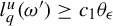 $l^{u}_{q}(\omega ')\geq c_{1}\theta _{\epsilon }$
. Thus, in turn, there exists
 $\omega ^{u}\in W^{u}_{q}(\omega ')$
such that
 $$ \begin{align*} B^{u}\bigg(\omega^{u}, \frac{c_{1}\theta_{\epsilon}}{3}\bigg)\subset W^{u}_{q}(\omega'). \end{align*} $$
Similarly, using the definitions of
 $n_{2}(\omega )$
and
 $l^{s}_{q'}$
, there exist
 $\omega "\in \Sigma _{A}$
,
 $c_{2}>0$
such that
 $l^{s}_{q'}(\omega ")\geq c_{2}\theta _{\epsilon }$
, and
 $\omega ^{s}\in W^{s}_{q'}(\omega ")$
such that
 $B^{s}(\omega ^{s},{(c_{2}\theta _{\epsilon })}/{3})\subset W^{s}_{q'}(\omega ).$
Let
 ${k>{3c_{\mathrm {L}}}/{(\min (c_{1},c_{2}))}}$
. Set
 $\omega _{i}\in \Sigma _{A}$
such that
 $\chi (\omega _{i})=\{\omega ^{s},\omega ^{u}\}$
. Then, using Lemma 2.11, we get
 $$ \begin{align*} B\bigg(\chi(\omega_{i}),\frac{\theta_{\epsilon}}{k}\bigg)\subset C_{-q,q'}, \end{align*} $$
which finishes the proof.
Set
 $\mathcal {P}_{\epsilon }=\{\mathcal {P}_{\epsilon ,i,j}\mbox { : } i=1,\ldots ,N_{\epsilon }; j\geq 0, D_{\epsilon ,i}\times [j\theta _{\epsilon },(j+1)\theta _{\epsilon }[\ \subset \Delta \}$
. We will consider the elements of
 $\mathcal {P}_{\epsilon }$
which intersect the boundary of
 $\Delta $
, thus we consider the set
 $$ \begin{align*} \bar{\mathcal{P}}_{\epsilon}:=\{\mathcal{P}_{\epsilon,i,j}\mbox{ : } i=1,\ldots,N_{\epsilon}; j\geq0, D_{\epsilon,i}\times[j\theta_{\epsilon},(j+1)\theta_{\epsilon}[\ \cap\ \partial\Delta\neq\emptyset\}. \end{align*} $$
In the following lemma, we show that the measure of the union of the elements of
 $\bar {\mathcal {P}}_{\epsilon }$
can be neglected in our study.
Lemma 5.3. The
 $\nu $
-measure of the union of the elements of
 $\bar {\mathcal {P}}_{\epsilon }$
is
 $O(\theta _{\epsilon })$
.
Proof. Let
 $P\in \bar {\mathcal {P}}_{\epsilon }$
. Then according to Lemma 5.1, P is contained in the
 $\theta _{\epsilon }$
-neighborhood of the graph of
 $r:\Sigma _{A}\rightarrow [0,+\infty ]$
. So
 $$ \begin{align*} \bigcup_{P\in \bar{\mathcal{P}}_{\epsilon}} P\subset\{(\omega,s)\in\Delta: r(\omega)-\theta_{\epsilon}<s\leq r(\omega)\}, \end{align*} $$
whose measure (with respect to
 $\mu _{\Delta }$
) is bounded by
 ${\theta _{\epsilon }}/{(\int _{\Sigma _{A}}r\,d\nu )}$
.
From now on, let us set
 $A_{\epsilon }(y):=\chi ^{-1}(P_{D}(B(y,\epsilon )))$
. We denote respectively by
 $A_{\epsilon -\theta _{\epsilon }}(y_{\epsilon ,i,j})$
and
 $A_{\epsilon +\theta _{\epsilon }}(y_{\epsilon ,i,j})$
the projections of the balls
 $B(y_{\epsilon ,i,j},\epsilon -\theta _{\epsilon })$
and
 $B(y_{\epsilon ,i,j},\epsilon +\theta _{\epsilon })$
on
 $\Sigma _{A}$
, and we set
 $A_{\epsilon }^{-}=\bigcup _{k\in I}D_{\epsilon ,k}$
and
 $A^{+}_{\epsilon }=\bigcup _{l\in J}D_{\epsilon ,l}$
, where
 $I=\{k: D_{\epsilon ,k}\subset A_{\epsilon -\theta _{\epsilon }}(y_{\epsilon ,i,j})\}$
and
 $J=\{l:D_{\epsilon ,l}\cap A_{\epsilon +\theta _{\epsilon }}(y_{\epsilon ,i,j})\neq \emptyset \}$
. Then we have the following inclusions for
 $y\in \mathcal {P}_{\epsilon ,i,j} $
:
 $$ \begin{align} A_{\epsilon}^{-}(y_{\epsilon,i,j})\subset A_{\epsilon-\theta_{\epsilon}}(y_{\epsilon,i,j})\subset A_{\epsilon}(y)\subset A_{\epsilon+\theta_{\epsilon}}(y_{\epsilon,i,j})\subset A_{\epsilon}^{+}(y_{\epsilon,i,j}). \end{align} $$
Let
 $y\in M$
. If
 $\epsilon>0$
is small enough,
 $y\in \bigcup _{P\in \mathcal {P}_{\epsilon }}P$
, there exists
 $i,j$
such that
 $y\in \mathcal {P}_{\epsilon ,i,j}$
. Consider the ball
 $B(y,\epsilon )$
, and let
 $y_{\epsilon ,i,j}\in \mathcal {P}_{\epsilon ,i,j}$
. We have
 $$ \begin{align} B(y_{\epsilon,i,j},\epsilon-\theta_{\epsilon})\subset B(y,\epsilon)\subset B(y_{\epsilon,i,j},\epsilon+\theta_{\epsilon}). \end{align} $$
This comes from the fact that the diameter of
 $\mathcal {P}_{\epsilon ,i,j}$
is bounded by
 $\theta _{\epsilon }$
. Furthermore, after projecting on
 $\Sigma _{A}$
, let
 $x_{\epsilon ,i}\in X$
such that
 $x_{\epsilon ,i}=\chi (\omega _{\epsilon ,i})$
. We note that there exist
 $\alpha _{1}$
,
 $\alpha _{2}>0$
, such that
 $$ \begin{align} \nu(\chi^{-1}(B(x_{\epsilon,i}, \alpha_{1}\epsilon)))\leq \nu(A_{\epsilon}(y_{\epsilon,i,j}))\leq \nu(\chi^{-1}(B(x_{\epsilon,i},\alpha_{2}\epsilon))). \end{align} $$
In what follows, we consider the notation
 $$ \begin{align*}A_{\epsilon}^{-}(y):=A_{\epsilon}^{-}(y_{\epsilon,i,j})\mbox{, } A_{\epsilon}^{+}(y):=A^{+}_{\epsilon}(y_{\epsilon,i,j}) \quad\text{and}\quad D_{\epsilon}(x):=D_{\epsilon,i},\end{align*} $$
where x is the point of X such that
 $y=g_{s}(x)$
for some
 $s\in [0,R(x)[$
and if
 $y\in B(y_{\epsilon ,i,j},\epsilon )$
.
Proposition 5.4. Recall that a measure
 $\nu $
on a metric space is called Federer if there exists a constant
 $c_{F}>0$
such that for any point x and any
 $r>0$
,
 $$ \begin{align*} \nu(B(x,2r))\leq c_{F}\nu(B(x,r)). \end{align*} $$
Remark 5.5. By Theorem 5.1 in [Reference Pesin and Sadovskaya17], the measure
 $\nu $
is Federer. By direct induction, for all
 $m\geq 0$
,
 $$ \begin{align} \nu(B(x,2^{m}r))\leq c_{F}^{m}\nu(B(x,r)). \end{align} $$
We will show a result of convergence in distribution for
 $\tau _{\epsilon }$
. We will start by proving the following two lemmas.
Lemma 5.6. There exist
 $\eta _{0}>0$
and
 $\epsilon>0$
such that if
 $ {\delta }/{\epsilon } <\eta _{0}$
, for any
 $x\in (\partial A_{\epsilon }(y))^{[\delta ]}$
, then there exists
 $z\in \partial A_{\epsilon }(y)$
, such that
 $z\in W^{u}(x)$
or
 $W^{s}(x)$
.
Proof. This comes from the transversality of
 $W^{s}(x)$
and
 $W^{u}(x)$
and the fact that
 $\partial A_{\epsilon }(y)$
is
 $C^{1}$
of order
 ${1}/{\epsilon }$
.
Lemma 5.7. For all
 $\epsilon>0$
, the
 $\nu $
-measures of the sets
 $A_{\epsilon }^{+}(y)$
and
 $A_{\epsilon }^{-}(y)$
are equivalent.
Proof. We know that the cylinders of
 $\mathcal {D}_{\epsilon }$
are of diameter less than
 $\theta _{\epsilon }$
, and the projection map on
 $\Sigma _{A}$
is Lipschitz with constant
 $k_{\mathrm {L}}$
. Set
 $\delta =(k_{\mathrm {L}}+1)\theta _{\epsilon }$
and let
 $k_{0}$
be the smallest positive number satisfying
 $k_{\mathrm {L}} \epsilon +\delta + \epsilon \leq k_{0}\epsilon $
. By the coding map
 $\chi $
, we have on the Poincaré section X that
 $$ \begin{align*} A_{\epsilon}^{+}(y)\backslash A_{\epsilon}^{-}(y)&=A_{\epsilon}(y)^{[(k_{\mathrm{L}}+1)\theta_{\epsilon}]}\cap (X\backslash A_{\epsilon}(y))^{[(k_{\mathrm{L}}+1)\theta_{\epsilon}]}\\ &=(\partial A_{\epsilon}(y))^{[\delta]}, \end{align*} $$
thus we need to prove that the measure of the
 $\delta $
-neighborhood of
 $A_{\epsilon }(y)$
is negligible with respect to the measure of
 $A_{\epsilon }(y)$
. Indeed, let
 $m_{F}>0$
be such that
 $k_{0}\leq 2^{m_{F}}\alpha _{1}$
. Then, using the Federer property (Remark 5.5) and the inclusion in (5.4), there exists
 $c_{F}>0$
such that
 $$ \begin{align} \nu(\chi^{-1}(B(x, k_{0}\epsilon)))\leq c_{F}^{m_{F}}\nu(\chi^{-1}(B(x,\alpha_{1}\epsilon)))\leq c_{F}^{m_{F}}\nu(A_{\epsilon}(x)), \end{align} $$
hence it is sufficient to prove that
 $\nu ((\partial A_{\epsilon }(y))^{[\delta ]})$
is negligible with respect to
 $\nu (\chi ^{-1}(B(x, k_{0}\epsilon )))$
.
Now, due to Lemma 5.6, we will work on two parts of
 $\partial A_{\epsilon }(y)^{[\delta ]}$
.
Let
 $x_{0}$
be a point in D. Let
 $x\in W^{s}(x_{0})$
. We set
 $I^{u}(x):=W^{u}_{\mathrm {loc}}(x)\cap (\partial A_{\epsilon }(y))^{[\delta ]}$
such that, for all
 $\xi _{x}\in I^{u}(x)$
, there exists
 $z\in \partial A_{\epsilon }$
as in Lemma 5.6 and where
 $z\in W^{u}(\xi _{x})$
. On the other hand, we set
 $I^{s}(x):=W^{s}_{\mathrm {loc}}(x)\cap (\partial A_{\epsilon }(y))^{[\delta ]}$
, such that, for all
 $ \xi _{x}'\in I^{s}(x)$
, there exists
 $z'\in \partial A_{\epsilon }$
as in Lemma 5.6 and where
 $z'\in W^{s}(\xi _{x}')$
.
Hence, we have
 $\partial A_{\epsilon }(y)^{[\delta ]}=\mathcal {I}^{u}\cup \mathcal {I}^{s}$
, where
 $$ \begin{align*} \mathcal{I}^{u}:=\bigcup_{x\in W^{s}(x_{0})}I^{u}(x) \quad\text{and}\quad \mathcal{I}^{s}:=\bigcup_{x\in W^{s}(x_{0})}I^{s}(x). \end{align*} $$
Our aim is to estimate the measure of
 $\mathcal {I}^{u}$
with respect to that of
 $B(x, k_{0}\epsilon )$
. We will start working on
 $\nu ^{u}(\pi ^{+}(\chi ^{-1}(I^{u})))$
and then after integrating over
 $\Sigma _{A}^{-}\times \Sigma _{A}^{+}$
, we will conclude the estimation of
 $\nu (\chi ^{-1}(\mathcal {I}^{u}))$
.
Let
 $q_{i}$
be the greatest integer such that
 $l^{u}_{q_{i}}(\omega _{i})>3c\delta $
. Then we have
 $$ \begin{align*} I^{u}(x)\subset \bigcup_{i=1}^{2}\chi(C_{-\infty,q_{i}}(\omega_{i}))\subset B(x,k_{0}\epsilon), \end{align*} $$
and so
 $\nu ^{u}(\pi ^{+}(\chi ^{-1}(I^{u})))\leq \sum _{i=1}^{2}\nu ^{u}(C_{0,q_{i}}(\pi ^{+}(\omega _{i})))$
. Knowing that
 $W^{u}(x)= \chi (C_{-\infty ,0}(\omega )) =\bigcap _{i=1}^{\infty }\chi (C_{-i, 0}(\omega ))$
, let
 $p_{i}$
be the smallest integer such that
 $$ \begin{align*} \prod_{k=0}^{p_i -1}(\mathbf{a}^{u}(\sigma^{k}(\omega_i)))^{-1}> k_{0}\epsilon, \quad \prod_{k=0}^{p_i}(\mathbf{a}^{u}(\sigma^{k}(\omega_i)))^{-1} \leq k_{0}\epsilon. \end{align*} $$
Then using Proposition 2.7, we have
 $$ \begin{align} \chi(C_{-\infty, p_{i}}(\omega))\subset W^{u}(x)\cap B(x,k_{0}\epsilon), \end{align} $$
but
 $\nu ^{u}(C_{0,p_{i}}(\pi ^{+}(\omega _{i})))\leq \nu ^{u}(\pi ^{+}(\chi ^{-1}(B(x, k_{0}\epsilon )\cap W^{u}(x))))$
, thus, since
 $\nu ^u$
is a Gibbs measure (see (2.11) and (2.5)), by Proposition 2.2 there exists a constant
 $k_{\tilde {h}}\geq 1$
, and knowing that
 $\max {\tilde {h}}<-\gamma $
for some
 $\gamma>0$
, we get
 $$ \begin{align*} \frac{\nu^{u}(\pi^{+}(\chi^{-1}(I^{u})))}{\nu^{u}(\pi^{+}(\chi^{-1}(B(x, k_{0}\epsilon)\cap W^{u}(x))))}&\leq \sum_{i=1}^{2}\frac{\nu^{u}(C_{0,q_{i}}(\pi^{+}(\omega_{i})))}{\nu^{u}(C_{0,p_{i}}(\pi^{+}(\omega_{i})))}\\ &\leq \sum_{i=1}^{2} k^{2}_{\tilde{h}} \exp\bigg(\sum_{k=p_{i}}^{q_{i}-1}\tilde{h}(\sigma^{k}(\omega_{i}))-(p_i -q_i)P_\sigma(\tilde{h})\bigg)\\ &\leq \sum_{i=1}^{2} k^{2}_{\tilde{h}} \exp((-\gamma+P_{\sigma}(\tilde{h}))(q_{i}-p_{i}))\\ &\leq\eta(\epsilon), \end{align*} $$
where
 $\eta (\epsilon )\rightarrow 0$
as
 $\epsilon $
goes to 0, since
 $q_{i}=o(p_{i})$
, and
 $p_{i}\rightarrow \infty $
. Set
 $\tilde {I^{u}}=\{(\omega ^{-}, \omega ^{+}): \text { there exists } \omega =(\omega _{n})_{n\in \mathbb {Z}}\in \Sigma _{A} \mbox { such that } \chi (\omega )\in I^{u}, \omega ^{-}=(\omega _{n})_{n\leq 0} \text { and } \omega ^{+}= (\omega _{n})_{n\geq 0}\}$
, and in the same way we define the set
 $\tilde {B}(x, k_{0}\epsilon )$
. We have

On the other hand, the measure
 $\nu $
is absolutely continuous with respect to the product measure
 $\nu ^{u}\otimes \nu ^{s}$
with bounded density function h (see Proposition 2.3 in [Reference Pesin and Sadovskaya17]). Then there exist
 $\kappa _{1}$
,
 $\kappa _{2}>0$
such that, using the previous inequality, we get

where
 $\tilde {\eta }(\epsilon )=({\kappa _{2}}/{\kappa _{1}})\eta (\epsilon )$
.
Proceeding with the same strategy as above, there exists
 $\bar {\eta }(\epsilon )$
such that
 $\nu (\chi ^{-1}(\mathcal {I}^{s}))\leq \bar {\eta }(\epsilon )\nu (\chi ^{-1}(B(x,k_{0}\epsilon )))$
, and this finishes the proof since
 $\tilde {\eta }(\epsilon )$
and
 $\bar {\eta }(\epsilon )$
go to 0 as
 $\epsilon \rightarrow 0$
.
Definition 5.8. We fix
 $y\in \Sigma _{A}$
. For
 $x\in A_{\epsilon }(y)$
, we define the first return time to
 $A_{\epsilon }(y)\times \{0\}$
in
 $\Sigma _{A}\times \mathbb {Z}$
by
 $$ \begin{align*} w_{A_{\epsilon}(y)}(x) =\inf\{n\geq1, S_{n}\varphi(x)=0 \text{ and } \sigma^{n}x\in A_{\epsilon}(y)\}. \end{align*} $$
We define in the same way
 $w_{A_{\epsilon }^{\pm }(y)}(x)=\min \{n\geq 1 : \sigma ^{n}(x)\in A_{\epsilon }^{\pm }(y)\}$
, the first return time of a point x into
 $A_{\epsilon }^{+}(y)$
.
Remark 5.9. We will start by studying the asymptotic behavior of
 $w_{A_{\epsilon }(y)}(x)$
to deduce that of
 $\tau _{\epsilon }(x)$
.
Proposition 5.10. For every
 $y\in M$
, every
 $\epsilon>0$
, consider
 $n_\epsilon =n_\epsilon (t,y):= ({t}/{\nu (A_{\epsilon }^{\pm }(y))})^{2}$
and
 $M_\epsilon $
and
 $Q_\epsilon $
as defined in (5.1). Let D be a set satisfying either (
 $D\in \mathcal {D}_{\epsilon }$
and
 $D\subset A_{\epsilon }^{\pm }(y)$
) or
 $D=A_{\epsilon }^{\pm }(y)$
. We have
-
(a)
$1\geq \nu (w_{A_{\epsilon }^{\pm }(y)}>n_{\epsilon }|D)+{1}/{\big (\!\sqrt {2\pi }\sigma _{\varphi }\big )}\sum _{r=M_{\epsilon }}^{n_{\epsilon }}{\nu (A_{\epsilon }^{\pm }(y)\cap \{w_{A_{\epsilon }^{\pm }(y)}>n_{\epsilon }-r\})}/ {\sqrt {r-Q_{\epsilon }}}-o(1)$
, -
(b)
$1\leq \nu (w_{A_{\epsilon }^{\pm }(y)}>n_{\epsilon }|D)+{1}/{\big (\!\sqrt {2\pi }\sigma _{\varphi }\big )}\sum _{r=M_{\epsilon }}^{n_{\epsilon }}{\nu (A_{\epsilon }^{\pm }(y)\cap \{w_{A_{\epsilon }^{\pm }(y)}>n_{\epsilon }-r\})}/ {\sqrt {r-Q_{\epsilon }}}+ \nu (w_{A_{\epsilon }^{\pm }(y)}\leq M_{\epsilon }|D)+o(1)$
.


Proof. We use the same method as Dvoretzky and Erdös in [Reference Dvoretzky and Erdös9, Reference Pène and Saussol12, Reference Pène and Saussol13, Reference Pène, Saussol and Zweimüller15]. We make a partition of the cylinder D according to the last passage
 $r\leq n$
in the time interval
 $0,\ldots ,n$
of the orbit of
 $(x,0)$
by the map
 $\tilde {T}$
into
 $A_{\epsilon }^{\pm }(y)\times \{0\}$
. This can be seen as follows.
For simplicity, we will write
 $A_{\epsilon }^{\pm }$
instead of
 $A_{\epsilon }^{\pm }(y)$
:
 $$ \begin{align} \nu(D)=\sum_{r=0}^{n}& \nu(x\in D;S_{r}\varphi(x)=0\mbox{, } \sigma^{r}(x)\in A_{\epsilon}^{\pm};\text{ for all }\nonumber\\ & \quad l=r,\ldots,n, S_{l}\varphi(x)\neq0 \text{ or } \sigma^{l}(x)\notin A_{\epsilon}^{\pm}). \end{align} $$
Knowing that
 $S_{r}\varphi (x)=0$
, then
 $$ \begin{align*} \{\text{for all } l=r,\ldots,n, S_{l}\varphi(x)-S_{r}\varphi(x)\neq0 \mbox{ or } \sigma^{l}(x)\notin A_{\epsilon}^{\pm}\} \end{align*} $$
is equal to
 $$ \begin{align*} \{\text{for all } k=1,\ldots,n-r, S_{k+r}\varphi(x)-S_{r}\varphi(x)\neq0 \mbox{ or } \sigma^{k+r}(x)\notin A_{\epsilon}^{\pm}\}, \end{align*} $$
but
 $S_{k+r}\varphi (x)-S_{r}\varphi (x)=\sum _{l=0}^{k-1}\varphi \circ \sigma ^{l+r}(x)=S_{k}\varphi (\sigma ^{r}x)$
. It follows that
 $\nu (D)$
is equal to
 $$ \begin{align*} &\sum_{r=0}^{n} \nu(x\in D;S_{r}(x)=0,\sigma^{r}(x)\in A_{\epsilon}^{\pm}; \sigma^{-r}\{z\in\Sigma_{A}: \text{for all }\\& \qquad k=1,\ldots,n-r, S_{k}\varphi(z)\neq0,\sigma^{k}(z)\notin A_{\epsilon}^{\pm}\}), \end{align*} $$
from which we get
 $$ \begin{align*} \nu(D)&=\sum_{r=0}^{n}\nu(D\cap\{S_{r}=0\}\cap \sigma^{-r}(A^{\pm}_{\epsilon}\cap\{w_{A^{\pm}_{\epsilon }}>n-r\}))\\&\geq \nu(D\cap A^{\pm}_{\epsilon}\cap\{w_{A^{\pm}_{\epsilon}}>n\})\\&\quad +\sum_{r=2q+1}^{n}\nu(D\cap\{S_{r}=0\}\cap \sigma^{-r}(A_{\epsilon}^{\pm}\cap\{w_{A_{\epsilon}^{\pm}}(x)>n-r\})). \end{align*} $$
Recall that D is a
 $(-q, q')$
-cylinder with
 $q\leq Q_{\epsilon }$
, and
 $A_{\epsilon }^{\pm }$
is a union of
 $(-Q_{\epsilon }, q")$
-cylinders for some
 $q">0$
. Let
 $E=A_{\epsilon }^{\pm }(y)\cap \{w_{A_{\epsilon }^{\pm }}>n\}$
be the set of points of
 $A_{\epsilon }^{\pm }(y)$
which do not return to
 $A_{\epsilon }^{\pm }$
before n, that is,
 $E=A_{\epsilon }^{\pm }\cap \bigcap _{s=1}^{n}(\{S_{s}\varphi \neq 0\}\cup \sigma ^{-s}(\Sigma _{A}\setminus A_{\epsilon }^{\pm }))$
.
We know that
 $\varphi $
is constant on
 $1$
-cylinders, then
 $\{S_{s}\varphi \neq 0\}$
is a union of s-cylinders, and
 $\sigma ^{-s}(\Sigma _{A}\setminus A_{\epsilon }^{\pm })=\Sigma _{A}\setminus \sigma ^{-s}(A_{\epsilon }^{\pm })$
is a union of
 $(-Q_{\epsilon }+s,q"+s)$
-cylinders. Then we get that E is a union of
 $(-Q_{\epsilon }, q")$
-cylinders, for some
 $q">0$
. Hence, E can be written as
 $\sigma ^{Q_{\epsilon }}({\Pi _{+}}^{-1}B)$
, where B is a subset of
 $\Sigma _{A}^{+}$
, and
 $\Pi _{+}$
is the canonical projection of
 $\Sigma _{A}$
on
 $\Sigma _{A}^{+}$
.
Now let
 $n=n_{\epsilon }$
. With all these conditions, we apply the local limit theorem in Proposition 4.3. Thus, there is
 $C_{1}>0$
such that
 $$ \begin{align*} \nu(D) &\geq\nu(D\cap\{w_{A_{\epsilon}^{\pm}}(x)>n_{\epsilon}\})+\sum_{r=M_{\epsilon}}^{n_{\epsilon}}\frac{\nu(D)\nu(A_{\epsilon}^{\pm}\cap\{w_{A_{\epsilon}^{\pm}}(x)>n_{\epsilon}-r\})}{\sqrt{2\pi}\sqrt{r-(Q_{\epsilon}+l)}\sigma_{\varphi}}\\&\quad - C_{1}\sum_{r=M_{\epsilon}}^{n_{\epsilon}}\frac{\nu(A_{\epsilon}^{\pm}\cap\{w_{A_{\epsilon}^{\pm}}(x)>n_{\epsilon}-r\})Q_{\epsilon}\nu(D)}{r-2Q_{\epsilon}}. \end{align*} $$
There is
 $C_{3}>0$
such that the error term is controlled by
 $$ \begin{align} \sum_{r=M_{\epsilon}}^{n_{\epsilon}}\frac{\nu(A_{\epsilon}^{\pm})q\nu(D)}{r-2Q_{\epsilon}}\leq C_{3}Q_{\epsilon}\log{n_{\epsilon}}\nu(D)\nu(A_{\epsilon}^{\pm}), \end{align} $$
since
 $Q_{\epsilon }\nu (A_{\epsilon }^{\pm })\log {n_{\epsilon }}=o(1)$
, hence we get
 $$ \begin{align*} \nu(D)&\geq \nu(D\cap\{w_{A^{\pm}_{\epsilon}}(x)>n_{\epsilon}\}) +\nu(D)\sum_{r=M_{\epsilon}}^{n_{\epsilon}}\frac{\nu(A_{\epsilon}^{\pm}\cap\{w_{A_{\epsilon}^{\pm}}(x)>n_{\epsilon}-r\}}{\sqrt{2\pi}\sqrt{r-Q_{\epsilon}}\sigma_{\varphi}}\\&\quad -o(\nu(D)), \end{align*} $$
and thus dividing by
 $\nu (D)$
yields (a) for
 $D\in \mathcal {D}_{\epsilon }$
such that
 $D\subset A_{\epsilon }^{\pm }(y)$
.
We prove inequality (b) following the same strategy. For
 $n_{\epsilon }=({t}/{\nu (A_{\epsilon }^{\pm }(y))})^{2}$
, using the same decomposition as in (5.8), we have
 $$ \begin{align*} \nu(D)=\sum_{r=0}^{n_{\epsilon}}\nu(D\cap\{S_{r}=0\}\cap \sigma^{-r}(A_{\epsilon}^{\pm}(y)\cap\{w_{A^{\pm}_{\epsilon}(y)}(x)>n_{\epsilon}-r\})):=\sum_{r=0}^{n_{\epsilon}}G_{r,\epsilon}(x). \end{align*} $$
For
 $r=0$
, the first term is equal to
 $\nu (D\cap \{w_{A^{\pm }_{\epsilon }(y)}(x)>n_{\epsilon }\})$
. We then compute the sum of terms between 1 and
 $M_{\epsilon }$
:
 $$ \begin{align*} &\sum\limits_{r=1}^{M_{\epsilon}}\nu(D\cap\{S_{r}=0\}\cap \sigma^{-r}(A_{\epsilon}^{\pm}(y)\cap\{w_{A_{\epsilon}^{\pm}(y)}>n_{\epsilon}-r\}))\\ &\quad= \nu\bigg(\bigcup_{r=1}^{M_{\epsilon}} D\cap\{S_{r}=0\}\cap \sigma^{-r}(A_{\epsilon}^{\pm}(y)\cap\{w_{A_{\epsilon}^{\pm}(y)}>n_{\epsilon}-r\})\bigg)\\&\quad\leq\nu(D\cap\{w_{A_{\epsilon}^{\pm}(y)}\leq M_{\epsilon}\}). \end{align*} $$
Then, using the local limit theorem in Proposition 4.3, there exists
 $C_{4}>0$
such that we have
 $$ \begin{align*} \sum^{n_{\epsilon}}_{r=M_{\epsilon}} G_{r,\epsilon}(x)&\leq \frac{1}{\sqrt{2\pi}\sigma_{\varphi}}\sum^{n_{\epsilon}}_{r=M_{\epsilon}}\frac{\nu(D)\nu(A^{\pm}_{\epsilon}\cap\{w_{A_{\epsilon}^{\pm}}>n_{\epsilon}-r\})}{\sqrt{r-Q_{\epsilon}}}\\& \quad +C_{4}\frac{\nu(A^{\pm}_{\epsilon}\cap\{w_{A_{\epsilon}^{\pm}}>n_{\epsilon}-r\})Q_{\epsilon}\nu(D)}{r-2Q_{\epsilon}}. \end{align*} $$
Similarly as in (5.9), the error term is controlled by
 $o(\nu (D))$
. Combining these assumptions together, we obtain
 $$ \begin{align} \nu(D)&\leq o(\nu(D))+\nu(D\cap\{w_{A_{\epsilon}^{\pm}}>n_{\epsilon}\})+\nu(w_{A_{\epsilon}^{\pm}}\leq M_{\epsilon}|D)\nu(D)\nonumber\\&\quad +\frac{1}{\sqrt{2\pi}\sigma_{\varphi}}\nu(D)\nu(A^{\pm}_{\epsilon}\cap\{w_{A_{\epsilon}^{\pm}}>n_{\epsilon}\})\bigg(\sum^{n_{\epsilon}}_{r=M_{\epsilon}}\frac{1}{\sqrt{r-Q_{\epsilon}}}\bigg). \end{align} $$
Dividing by
 $\nu (D)$
yields the desired inequality.
Corollary 5.11. Under the hypothesis of Proposition 5.10, where
 $n_{\epsilon }$
,
 $M_{\epsilon }$
and D are considered similarly, we have:
-
(a)
$1+o(1)= \nu (w_{A_{\epsilon }^{\pm }(y)}\!>n_{\epsilon }|D)+{1}/{(\sqrt {2\pi }\sigma _{\varphi })} \sum _{r=M_{\epsilon }}^{n_{\epsilon }}(\nu (A_{\epsilon }^{\pm }(y)\cap \{w_{A_{\epsilon }^{\pm }(y)}\!> n_{\epsilon }-r\}))/{(\sqrt {r-Q_{\epsilon }})} +O(\nu (w_{A_{\epsilon }^{\pm }(y)}\leq M_{\epsilon }|D));$
-
(b)
$1+o(1) = \nu (w_{A_{\epsilon }^{\pm }(y)}> n_{\epsilon }|A_{\epsilon }^{\pm }(y)) + {1}/{(\sqrt {2\pi } \sigma _{\varphi })} \sum _{M_{\epsilon }}^{n_{\epsilon }} (\nu (A_{\epsilon }^{\pm }(y)\cap \{ w_{A_{\epsilon }^{\pm }(y)}> n_{\epsilon }-r\}))/ {(\sqrt {r-Q_{\epsilon }})}+O(\nu (w_{A_{\epsilon }^{\pm }(y)} \leq M_{\epsilon }|A_{\epsilon }^{\pm }(y))).$


Lemma 5.12. From the previous corollary, we have
 $$ \begin{align*} \nu(w_{A_{\epsilon}^{\pm}(y)}>n_{\epsilon}|D)=\ &\nu(w_{A_{\epsilon}^{\pm}(y)}>n_{\epsilon}|A_{\epsilon}^{\pm}(y))+O(\nu(w_{A_{\epsilon}^{\pm}(y)}\leq M_{\epsilon}|A_{\epsilon}^{\pm}(y)))\\ & +O(\nu(w_{A_{\epsilon}^{\pm}(y)}\leq M_{\epsilon}|D))+o(1). \end{align*} $$
Thus, we will study the convergence in distribution of
 $w_{A_{\epsilon }^{\pm }(y)}$
with respect to
 $\nu (\cdot|A_{\epsilon }^{\pm }(y))$
and then we will deduce it with respect to
 $\nu (\cdot|D)$
. So, first we have the following proposition.
Proposition 5.13. The family of distributions of
 $(\nu (A_{\epsilon }^{\pm }(y))^{2}w_{A_{\epsilon }^{\pm }(y)})_{\epsilon>0}$
is tight with respect to the family of probability measures
 $(\nu (\cdot|A_{\epsilon }^{\pm }(y)))_{\epsilon>0}$
.
Proof. Let
 $t>0$
. Using inequality (a) of Proposition 5.10 with
 $n_{\epsilon }=({t}/{\nu (A^{\pm }_{\epsilon }(y))})^{2}$
, we have
 $$ \begin{align*} 1&\geq\nu(w_{A_{\epsilon}^{\pm}(y)}>n_{\epsilon}|A^{\pm}_{\epsilon}(y))+\frac{1}{\sqrt{2\pi}\sigma_{\varphi}}\sum_{M_{\epsilon}}^{n_{\epsilon}}\frac{\nu(A_{\epsilon}^{\pm}(y)\cap \{w_{A_{\epsilon}^{\pm}(y)}>n_{\epsilon}-r\})}{\sqrt{r-Q_{\epsilon}}}- o(1)\\ &\geq\nu(w_{A_{\epsilon}^{\pm}(y)}>n_{\epsilon}|A^{\pm}_{\epsilon}(y))+\frac{1}{\sqrt{2\pi}\sigma_{\varphi}}\nu(A_{\epsilon}^{\pm}(y)\cap \{w_{A_{\epsilon}^{\pm}(y)}>n_{\epsilon}\})\sum_{M_{\epsilon}}^{n_{\epsilon}}\frac{1}{\sqrt{r-Q_{\epsilon}}}- o(1), \end{align*} $$
from which it follows that, for all
 $t>0$
,
 $$ \begin{align} \nu\bigg(\ w_{A_{\epsilon}^{\pm}(y)}>\bigg(\frac{t}{\nu(A^{\pm}_{\epsilon}(y))}\bigg)^{2}\bigg| A^{\pm}_{\epsilon}(y)\bigg)\leq \frac{1+o(1)}{1+{1}/({\sqrt{2\pi}\sigma_{\varphi}})\nu(A_{\epsilon}^{\pm}(y))\sum^{n_{\epsilon}}_{M_{\epsilon}} {1}/({\sqrt{r-Q_{\epsilon}}})}, \end{align} $$
but
 ${\sum }_{M_{\epsilon }}^{{n_{\epsilon }}}{1}/{(\sqrt {r-Q_{\epsilon }})}=2(\sqrt {n_{\epsilon }}-\sqrt {Q_{\epsilon }-M_{\epsilon }})\geq \sqrt {n_{\epsilon }}\geq ({t}/{\nu (A_{\epsilon }^{\pm }(y))})$
. Then we get
 $$ \begin{align} \underset{\epsilon\rightarrow0}{\limsup}\ \nu(\nu(A^{\pm}_{\epsilon}(y))^{2}w_{A_{\epsilon}^{\pm}(y)}>t^{2}\mid A^{\pm}_{\epsilon}(y))\leq\frac{1}{1+t}, \end{align} $$
which proves the tightness.
Theorem 5.14. [Reference Rousseau20]
Define
 $\bar {\tau _{\epsilon }}=\inf \{t>1: g_{t}(y)\in B(y,\epsilon )\}$
. For
 $\mu $
-almost every
 $y\in M$
,
 $$ \begin{align*} \underset{\epsilon\rightarrow0}{\lim}\ \frac{\log \bar{\tau_{\epsilon}}(y)}{-\log\epsilon}=\bar{d}-1, \end{align*} $$
where
 $\bar {d}$
is the Hausdorff dimension of the measure
 $\mu $
.
Consider the following lemma, where we will define a family of sets
 $D_{\epsilon }$
, and which we will apply later in our proofs with
 $D_{\epsilon }=A_{\epsilon }(y)$
and
 $D_{\epsilon }\in \mathcal {D}_{\epsilon }$
.
Lemma 5.15. For
 $\nu $
-almost every
 $x\in \Sigma _{A}$
, for all
 $k_{0}>0,m_{F}>0,c_{F}>0$
, let
 $(D_{\epsilon })_{\epsilon }$
be a family of sets containing x such that
 $D_{\epsilon }\subset B(x,k_{0}\epsilon )$
and
 $\nu (B(x, \mathrm {diam}(D_{\epsilon })))\leq c_{F}^{m_{F}}\nu (D_{\epsilon })$
. For
 $M_{\epsilon }$
defined as in (5.1), we have
 $$ \begin{align*} \underset{\epsilon\rightarrow0}{\lim}\ \nu(R_{B(x,k_{0}\epsilon)}\leq M_{\epsilon}|D_{\epsilon})=0, \end{align*} $$
where
 $R_{B(x, k_{0}\epsilon )}=\inf \{n\geq 1: \sigma ^{n}(x)\in B(x,k_{0}\epsilon )\}.$
Proof. Let
 $\alpha>0, k_{0}>0, m_{F}>0, c_{F}>0$
. Choose some
 $a\in (0,\alpha )$
and set, for some
 $\epsilon _{0}>0$
,
 $$ \begin{align*} F_{a}=\{x\in\Sigma_{A}:\text{ for all }\epsilon\leq\epsilon_{0},M_{\epsilon}^{-1}R_{B(x,2k_{0}\epsilon)}(x)>a\}. \end{align*} $$
We will show that
 $\nu (F_{a})\rightarrow 1$
as
 $\epsilon _{0}\rightarrow 0$
. To this end, let us prove that for
 $\nu $
-almost every
 $x\in \Sigma _{A}$
,
 $$ \begin{align} \underset{\epsilon\rightarrow0}{\lim}\ M_{\epsilon}^{-1}R_{B(x,2k_{0}\epsilon)}(x)=+\infty. \end{align} $$
An intermediate step in doing so is to prove that
 $$ \begin{align} \underset{\epsilon\rightarrow0}{\lim}\ \frac{\log R_{B(x,2k_{0}\epsilon)}}{-\log\epsilon}= \text{dim}_{\mathrm{H}}\mu-1, \quad \nu\mbox{-almost everywhere}. \end{align} $$
Let
 $r_{\min }>0$
and
 $r_{\max }>0$
the lower and upper bounds of the height function r. Using (4.3), for
 $\mu _{\Delta }$
-almost every
 $y=(x,s)\in \Delta $
, we have
 $$ \begin{align*} \bar{\tau_{\epsilon}}(y)\frac{1}{r_{\max}}\leq R_{B(x,2k_{0}\epsilon)}(x)\leq\bar{\tau_{\epsilon}}(y)\frac{1}{r_{\min}}, \end{align*} $$
which gives
 $$ \begin{align*} \frac{\log r_{\max}}{\log\epsilon}+\frac{\log\bar{\tau_{\epsilon}}(y)}{-\log\epsilon}\leq\frac{\log R_{B(x,2k_{0}\epsilon)}(x)}{-\log\epsilon}\leq \frac{\log r_{\min}}{\log\epsilon}+\frac{\log\bar{\tau_{\epsilon}}(y)}{-\log\epsilon}, \end{align*} $$
using Theorem 5.14. It follows that
 $\lim _{\epsilon \rightarrow 0}{(\log R_{B(x,2k_{0}\epsilon )})}/{(-\log \epsilon )}= \dim _{\mathrm {H}}\mu -1$
,
 $\nu $
-almost everywhere.
We now go back to show (5.13). Let
 $0<\delta _{0}<\dim _{\mathrm {H}}\mu -1$
, we have
 $$ \begin{align} \log(M_{\epsilon}^{-1}R_{B(x,2k_{0}\epsilon)}(x))=\log(M_{\epsilon}^{-1}\epsilon^{-\delta_{0}})+\log(\epsilon^{\delta_{0}}R_{B(x,2k_{0}\epsilon)}(x)). \end{align} $$
Note that the first term of (5.15) goes to
 $+\infty $
as
 $\epsilon $
goes to 0. This is true using the definition of
 $M_{\epsilon }$
. There exists
 $\rho _{0}>0$
such that
 $M_{\epsilon }<2 ({ |\!\log ({\theta _{\epsilon }}/{2Cc_{g}c_{l}})|}/{|\!\log \rho _{u}|})+1\leq \rho _{0}|\!\log \epsilon |$
, which is negligible with respect to
 $\epsilon ^{-\delta _{0}}$
.
Now, considering the second term, we observe that
 $$ \begin{align*} \frac{\log(\epsilon^{\delta_{0}}R_{B(x,2k_{0}\epsilon)}(x))}{-\log\epsilon}=-\delta_{0}+\frac{\log R_{B(x,2k_{0}\epsilon)}(x)}{-\log\epsilon}, \end{align*} $$
from which we get
 $$ \begin{align*}\log(\epsilon^{\delta_{0}}R_{B(x,2k_{0}\epsilon)}(x))\underset{\epsilon\rightarrow0}{\rightarrow} (-\delta_{0}+ {\dim}_{\mathrm{H}}\mu-1)(+\infty).\end{align*} $$
Therefore, (5.13) is proved.
Taking
 $\epsilon _{0}\rightarrow 0$
, by Egoroff’s theorem,
 $M_{\epsilon }^{-1}R_{B(x,2k_{0}\epsilon )}$
converges uniformly to
 $+\infty $
on
 $F_{a}$
, and
 $\nu (F_{a}^{C})\rightarrow 0$
.
Let
 $\epsilon <\epsilon _{0}$
. If
 $x'\in B(x,k_{0}\epsilon )$
and
 $R_{B(x,k_{0}\epsilon )}(x')\leq M_{\epsilon }$
, we have
 $R_{B(x,2k_{0}\epsilon )}(x')\leq M_{\epsilon }$
as well, hence
 $x'\in F_{a}^{C}$
. Therefore,
 $$ \begin{align*} D_{\epsilon}\cap\{x'\in\Sigma_{A},R_{B(x,k_{0}\epsilon)}(x')\leq M_{\epsilon}\}\subset D_{\epsilon}\cap F^{C}_{a}. \end{align*} $$
This means that for any density point x of the set
 $F_{a}$
relative to the Lebesgue basis given by
 $(B(\cdot,\delta ))_{\delta }$
,
 ${(\nu (F_{a}\cap B(x,\delta )))}/{(\nu (B(x,\delta )))}\rightarrow 1$
, as
 $\delta \rightarrow 0$
, and this is true for almost every point x. Therefore, we get
 $$ \begin{align*} \nu(R_{B(x,k_{0}\epsilon)}\leq M_{\epsilon}|D_{\epsilon})&\leq\nu(F_{a}^{C}|D_{\epsilon})\\ &=\frac{\nu(F^{C}_{a}\cap D_{\epsilon})}{\nu(D_{\epsilon})}\\ &\leq\frac{\nu(F^{C}_{a}\cap B(x,\text{diam}(D_{\epsilon})))}{\nu(D_{\epsilon})}\\ &\leq \nu(F^{C}_{a}| B(x,\text{diam}(D_{\epsilon})))\frac{\nu(B(x,\text{diam}(D_{\epsilon})))}{\nu(D_{\epsilon})}, \end{align*} $$
which converges to 0 as
 $\epsilon \rightarrow 0$
, since
 $\lim _{\epsilon \rightarrow 0} \nu (F_{a}^{C}|B(x,\text {diam} (D_{\epsilon })))=0$
and
 ${\nu (B(x,\text {diam}(D_{\epsilon }))}/{\nu (D_{\epsilon })}$
is bounded above by
 $c_{F}^{m_{F}}$
.
Proposition 5.16. For almost every
 $y\in M$
,
 $$ \begin{align*} \underset{\epsilon\rightarrow0}{\lim}\ \nu((\nu(A^{+}_{\epsilon}(y))^{2}w_{A^{+}_{\epsilon}(y)}>t|A_{\epsilon}^{+}(y))= \mathbb{P}\bigg(\sigma_{\varphi}^{2}\frac{\mathcal{E}^{2}}{\mathcal{N}^{2}}>t\bigg) \quad \text{for all } t>0, \end{align*} $$
and
 $$ \begin{align*} \underset{\epsilon\rightarrow0}{\lim}\ \nu((\nu(A^{-}_{\epsilon}(y))^{2}w_{A^{-}_{\epsilon}(y)}>t|A_{\epsilon}^{-}(y))= \mathbb{P}\bigg(\sigma^{2}_{\varphi}\frac{\mathcal{E}^{2}}{\mathcal{N}^{2}}>t\bigg) \quad \text{for all } t>0, \end{align*} $$
where
 $\mathcal {E}$
and
 $\mathcal {N}$
are independent random variables,
 $\mathcal {E}$
following the exponential distribution with mean 1 and
 $\mathcal {N}$
having the standard normal distribution.
Proof. After proving the tightness in Proposition 5.13, it will be enough to prove that the advertised limit is the only possible accumulation point of the distribution. Let
 $(\epsilon _{p})_{p\geq 1}$
be a positive sequence with
 $\lim _{p\rightarrow \infty } \epsilon _{p}=0$
and such that the conditional distribution of the
 $(\nu (A_{\epsilon _{p}}^{+})\sqrt {w_{A_{\epsilon _{p}}^{+}}}|A^{+}_{\epsilon _{p}})_{p\geq 0}$
converges to the law of some random variable
 $\mathcal {X}$
. Then, using Lemma 3.5 in [Reference Yassine23], it follows from Lemma 5.15 that
 $\mathcal {X}$
satisfies the integral equation
 $$ \begin{align} 1=\mathbb{P}(\mathcal{X}>t)+ t\frac{1}{\sqrt{2\pi}\sigma_{\varphi}}\int_{0}^{1}\frac{\mathbb{P}(\mathcal{X}>t\sqrt{1-u})}{\sqrt{u}}\,du \quad \text{for all } t>0. \end{align} $$
Then the conclusion follows as in Theorem 3.2 in [Reference Yassine23], the distribution of
 $\mathcal {X}$
coinciding with that of
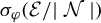 $\sigma _{\varphi }({\mathcal {E}}/{\mid \mathcal {N}\mid })$
.
Proposition 5.17. The family
 $(\nu (A_{\epsilon }(\cdot))^{2}\tau _{\epsilon })_{\epsilon }$
converges in distribution to
 $(\sigma ^{2}_{\varphi }\int _{X}\!R\,d\nu _{X}) ({\mathcal {E}^{2}}/{\mathcal {N}^{2}})$
with respect to any probability measure
 $\mathbb {P}$
absolutely continuous with respect to
 $\mu $
.
Proof. By density in
 $L^1(\mu )$
, it is enough to prove the result for
 $\mathbb P$
with density h such that
 $\sum _{k\in \mathbb {Z}} h\circ I^{k}$
is uniformly continuous on
 $\Lambda $
. Let
 $\tilde {\mu }=\nu \otimes {\mathrm {Leb}}\otimes \sum _{k\in \mathbb {Z}}\delta _{k}$
be the measure on
 $\tilde {M}$
. Set
 $\bar {\mu }:=\nu \otimes {\mathrm {Leb}}\otimes \delta _{0}$
the measure restricted on the 0-cell and let
 $\mathbb {P}$
be a probability measure absolutely continuous with respect to
 $\mu $
with a density function h. Set
 ${H(\cdot):=\sum _{k\in \mathbb {Z}}h(\cdot,k)}$
. By
 $\mathbb {Z}$
-periodicity, the distribution of
 $\tau _{\epsilon }$
under
 $\mathbb {P}$
is the same as under the probability measure absolutely continuous with respect to
 $\bar {\mu }$
with density H. We have
 $y=(x,s)\in \bigcup _{P\in \mathcal {P}_{\epsilon }}P$
, and there exist
 $i,j$
such that
 $y\in \mathcal {P}_{\epsilon ,i,j}$
. Let
 $y_{\epsilon ,i,j}\in \mathcal {P}_{\epsilon ,i,j}$
. Then
 $$ \begin{align*} H(y_{\epsilon,i,j})-w(H,\theta_{\epsilon})\leq H(y)\leq H(y_{\epsilon,i,j})+\omega(H,\theta_{\epsilon}), \quad y\in\mathcal{P}_{\epsilon,i,j}. \end{align*} $$
Then in turn
 $$ \begin{align} \underset{y\in\mathcal{P}_{\epsilon,i,j}}{\min}H(y)\geq H(y_{\epsilon,i,j})-\omega(H,\theta_{\epsilon}) \end{align} $$
and
 $$ \begin{align} \underset{y\in\mathcal{P}_{\epsilon,i,j}}{\max}H(y)\leq H(y_{\epsilon,i,j})-\omega(H,\theta_{\epsilon}). \end{align} $$
We are now in a position to proof our main result. For simplicity we will denote
 $A^{\pm }_{\epsilon ,i,j}:=A^{\pm }_{\epsilon }(y_{\epsilon ,i,j})$
. Due to (4.3) and Slutzky’s lemma, it is enough to prove that
 $(\nu (A_{\epsilon })(\cdot))^{2}w_{A_{\epsilon }(\cdot))}\circ P_{D}(\cdot))_{\epsilon }$
converges in distribution with respect to
 $(H\bar {\mu })$
to
 $\sigma _{\varphi }^{2}({\mathcal {E}^{2}}/{\mathcal {N}^{2}})$
.
For all
 $\epsilon>0$
,
 $\text { for all } t>0$
we set

Then, due to the inclusions in (5.2), for
 $y=(x,s)\in \mathcal {P}_{\epsilon ,i,j}$
,
 $$ \begin{align} \nu(A_{\epsilon,i,j}^{-})^{2}w_{A_{\epsilon,i,j}^{+}}(x)\leq\nu(A_{\epsilon}(x,s))^{2}w_{A_{\epsilon}(x,s)}(x)\leq\nu(A_{\epsilon,i,j}^{+})^{2}w_{A^{-}_{\epsilon,i,j}}(x), \end{align} $$
therefore, using inequality (5.18), we get

For all
 $y\in \mathcal {P}_{\epsilon ,i,j}$
, we have
 $A_{\epsilon }^{-}(y)=A_{\epsilon ,i,j}^{-}$
,
 $A_{\epsilon }^{+}(y)=A_{\epsilon ,i,j}^{+}$
, and
 $D_{\epsilon ,i}=D_{\epsilon }(x)$
. Then, for all
 $t>0$
,
 $$ \begin{align} E_{\epsilon,t}&\leq\sum_{i,j}H(y_{\epsilon,i,j})\int_{P_{i,j}}\nu(\nu(A_{\epsilon}^{+}(y))^{2}w_{A^{-}_{\epsilon}(y)}>t| D_{\epsilon}(x))\,d\bar{\mu}(y)+\omega(H,\theta_{\epsilon})\nonumber\\&\leq\int_{M}H(y)\nu(\nu(A_{\epsilon}^{+}(y))^{2}w_{A^{-}_{\epsilon}(y)}>t| D_{\epsilon}(x))\,d\bar{\mu}(y)+2\omega(H,\theta_{\epsilon}). \end{align} $$
We now have that
 $\nu (A^{-}_{\epsilon }(y))$
and
 $\nu (A_{\epsilon }^{+}(y))$
are equivalent (Lemma 5.7). Then there exists
 $\alpha (\epsilon )^{(y)}>0$
such that
 $\alpha (\epsilon )^{(y)}\rightarrow 0$
as
 $\epsilon \rightarrow 0$
and
 $$ \begin{align} \nu(A_{\epsilon}^{-}(y))(1-\alpha(\epsilon)^{(y)})\leq\nu(A_{\epsilon}^{+}(y))\leq\nu(A_{\epsilon}^{-}(y))(1+\alpha(\epsilon)^{(y)}), \end{align} $$
and, using Lemma 5.12, we get
 $$ \begin{align*} \nu(\nu(A_{\epsilon}^{+}(y))^{2}w_{A^{-}_{\epsilon}(y)}>t| D_{\epsilon}(x)) &\leq\nu((1+\alpha(\epsilon)^{(y)})^{2}\nu(A_{\epsilon}^{-}(y))^{2}w_{A^{-}_{\epsilon}(y)}>t| D_{\epsilon}(x))\\ &\leq\nu((1+\alpha(\epsilon)^{(y)})^{2}\nu(A^{-}_{\epsilon}(y))^{2}w_{A^{-}_{\epsilon}(y)}>t| A^{-}_{\epsilon}(y))\\ &\quad +\ \nu(w_{A_{\epsilon}^{-}(y)}\leq M_{\epsilon}|A_{\epsilon}^{-}(y))\\ &\quad -\nu(w_{A_{\epsilon}^{-}(y)}\leq M_{\epsilon}| D_{\epsilon}(x))+o(1). \end{align*} $$
Moreover, due to Lemma 5.15, applied with
 $A_{\epsilon }^{-}(y)$
and
 $D_{\epsilon }(x)$
, we have
 $\lim _{\epsilon \rightarrow 0} \nu (w_{A_{\epsilon }^{-}(y)} \leq M_{\epsilon }|A_{\epsilon }^{-}(y))=0$
, and
 $\lim _{\epsilon \rightarrow 0} \nu (w_{A_{\epsilon }^{-}(y)}\leq M_{\epsilon }| D_{\epsilon }(x))=0$
. And since H is uniformly continuous,
 $\lim {\epsilon \rightarrow 0} \omega (H,\nu _{\epsilon })=0$
. Thus, using the Lebesgue’s dominated convergence theorem in (5.21), we end up with
 $$ \begin{align} \underset{\epsilon\rightarrow0}{\limsup}\ E_{\epsilon,t}\leq \mathbb{P}\bigg(\bigg(\sigma^{2}_{\varphi}\int R\,d\nu_{X}\bigg)\frac{\mathcal{E}^{2}}{\mathcal{N}^{2}}>t\bigg) \quad \text{for all } t>0. \end{align} $$
We deal with the second inequality analogously; thus, using (5.17) and the first inequality in (5.20), we get

Similarly, due to Lemma 5.12, there exists
 $\alpha (\epsilon )^{(y)}>0$
such that
 $$ \begin{align*} & \nu(\nu(A_{\epsilon}^{-}(y))^{2}w_{A^{+}_{\epsilon}}>t| D_{\epsilon}(x)) \geq\nu\bigg(\frac{\nu(A^{+}_{\epsilon}(y))^{2}}{(1+\alpha(\epsilon)^{(y)})^{2}}w_{A^{+}_{\epsilon}}>t| A^{+}_{\epsilon}(y)\bigg)\\ &\quad+\ \nu(w_{A_{\epsilon}^{+}(y)}\leq M_{\epsilon}|A_{\epsilon}^{+}(y))-\nu(w_{A_{\epsilon}^{+}(y)} \leq M_{\epsilon}| D_{\epsilon}(x))+o(1). \end{align*} $$
Then, using Proposition 5.16, we get
 $$ \begin{align*} \underset{\epsilon\rightarrow0}{\lim}\ \nu\bigg(\frac{\nu(A^{+}_{\epsilon})^{2}}{(1+\alpha(\epsilon)^{(y)})^{2}}w_{A^{+}_{\epsilon}(y)}(x)>t| A^{+}_{\epsilon}(y)\bigg)=\mathbb{P}\bigg(\frac{\sigma^{2}_{\varphi}\mathcal{E}^{2}}{\mathcal{N}^{2}}>t\bigg) \quad \text{for all } t>0. \end{align*} $$
By using the same reasoning as demonstrated in the proof of (5.23), we can also establish that
 $$ \begin{align*} \underset{\epsilon\rightarrow0}{\liminf}\ E_{\epsilon,t}\geq \mathbb{P}\bigg(\sigma^{2}_{\varphi}\frac{\mathcal{E}^{2}}{\mathcal{N}^{2}}>t\bigg) \quad \text{for all } t>0. \end{align*} $$
Combining these results, we can deduce the convergence in law of
 $\nu (A_{\epsilon })^{2}w_{A_{\epsilon }(\cdot)}\circ P_{D}:\lim _{\epsilon \rightarrow 0} E_{\epsilon ,t}= \mathbb {P}(\sigma ^{2}_{\varphi }({\mathcal {E}^{2}}/{\mathcal {N}^{2}})>t)$
. Therefore, by applying Slutsky’s lemma, we obtain
 $$ \begin{align*} \underset{\epsilon\rightarrow0}{\lim} \ \mathbb{P}(\nu(A_{\epsilon}(\cdot))^{2}\tau_{\epsilon}(\cdot)>t)=\mathbb{P}\bigg(\bigg(\sigma^{2}_{\varphi}\int R\,d\nu_{X}\bigg)\frac{\mathcal{E}^{2}}{\mathcal{N}^{2}}>t\bigg) \quad \text{for all } t>0. \\[-41pt] \end{align*} $$
Theorem 3.2 follows from Proposition 5.17, combined with the fact that
 $\sigma _{\mathrm {flow}}^{2}={(\sigma _{\varphi }^{2})}/{(\int _{X}R\,d\nu _{X})}$
and the following lemma.
Lemma 5.18. For
 $\tilde {\nu }$
-almost every
 $\tilde {y}\in \tilde {M}$
, if
 $\tilde {D}_{0}$
is small enough, the measure
 $\tilde {\nu }_{0}$
given by (3.1) is well defined and
 $$ \begin{align*} \frac{\nu(A_{\epsilon}(y))}{\int_{X} R\,d\nu_{X}} \mbox{ is equivalent to } \tilde{\nu}^{y}_{0}(B(\tilde{y},\epsilon)), \end{align*} $$
with
 $y:=\Gamma (\tilde {y})\in M$
.
Proof. Let
 $\tilde {y}\in \tilde {M}$
. Note that since we are interested in the asymptotic behavior of
 $\tilde \nu _0(B(\tilde y,\epsilon ))$
when
 $\epsilon $
tends to
 $0$
, we can replace
 $\tilde D_0(\tilde y)$
by a smaller disk if we want.
If the disk
 $\tilde D_0(\tilde y)$
and
 $\epsilon $
are small enough, the image measure of
 $\tilde \mu ({\bigcup }_{-\epsilon <s<\epsilon }\tilde g_s (\tilde D_0(\tilde y)\cap \cdot ))$
by the projection of
 $\tilde M$
to M is equal to the measure
 $\mu ({\bigcup }_{-\epsilon <s<\epsilon }g_s(D_0(y) \cap \cdot )$
, where
 $D_0=D_0(y)$
is the disk around y obtained by the projection of the disk
 $\tilde D_0=\tilde D_0(\tilde y)$
.
So now we have to show that, for
 $\mu $
-almost every y in M, the measure
 $\tilde {\nu }_0^{y}$
defined on
 $D_0(y)$
by
 $$ \begin{align*} \tilde{\nu}_0^{y}(A)=\underset{\epsilon\rightarrow0}{\lim}\frac{1}{2\epsilon}\mu\bigg(\underset{-\epsilon<s<\epsilon}{\bigcup}g_{s}(D_{0}(y)\cap A)\bigg) \quad \text{for all } A\subset D_{0}(y), \end{align*} $$
is well defined and that
 $\tilde {\nu }_0^{y}(B(y,\epsilon ))$
is equivalent, as
 $\epsilon $
tends to 0, to
 $\nu (A_\epsilon (y))/\int _X R\,d\nu _{X}$
.
We assume that
 $y\in M\setminus X$
and that y is represented by a pair
 $(x,s)\in X_R$
with
 $x\not \in \partial X$
. Let us call D the connected component of X containing the point x. For
 $\epsilon $
small enough,
 $D_0(y)$
small enough,
 $\bigcup _{-\epsilon <s<\epsilon }g_s(D_0 (y))$
is contained in
 $\{(x',s')\in X_R\ :\ x\in D\}$
.
In
 $X_R$
, the set
 $D_0 (y)$
is represented by a curve
 $\{(x',h(x')) : x'\in P_{D}(D_0)\}$
with h of class
 $C^1$
of uniformly bounded derivative. We have, for every measurable set
 $A\subset D_0(y)$
,
 $$ \begin{align*} \mu\bigg(\underset{-\epsilon<s<\epsilon}{\bigcup}g_s(D_0(y) \cap A)\bigg) = \frac{2\epsilon \nu(\chi^{-1}( P_{D}(D_0(y)\cap A)))}{\int_X R\ d\nu_X} \end{align*} $$
This ensures the existence of
 $\nu _0$
and the fact that
 $$ \begin{align*} \nu_{0}^{y}(\cdot)=\frac{\nu(\chi^{-1}(P_{D}(\cdot\cap D_{0}(y))))}{\int_{X} R\,d\nu_{X}}. \end{align*} $$
We have to prove that
 $\nu (A_{\epsilon }(y))$
is equivalent to
 $\nu (\chi ^{-1}(P_{D}(B(y,\epsilon )\cap D_{0}(y))))$
. We observe that
 $D_{0}(y)\cap B(y,\epsilon )\subset B(y,\epsilon )$
. Therefore, we have
 $$ \begin{align*} A_{\epsilon}(y)=\chi^{-1}(P_{D}(B(y,\epsilon))))\supset \chi^{-1}(\Pi(D_{0}(y)\cap B(y,\epsilon))). \end{align*} $$
We need to prove that
 $\nu (A_\epsilon (y)) \setminus (\chi ^{-1}(P_{D}(D_0(y)\cap B(y,\epsilon ))))$
is negligible with respect to
 $\nu (A_\epsilon (y))$
.
We recall that
 $(x,s)\mapsto g_s(x)$
is a
 $C^1$
-diffeomorphism of
 $X_R$
on its image which contains the ball
 $B(y,\epsilon )$
, assuming
 $\epsilon $
is sufficiently small.
Let
 $z\in A_\epsilon (y) \setminus \chi ^{-1}(P_{D}(D_0(y)\cap B(y,\epsilon )))$
. Let us consider the point
 $z'=g_{h(z)}(\chi (z)) \in D_0\setminus B(y,\epsilon )$
. The diameter of
 $ A_\epsilon (y)$
is bounded by
 $C_y\epsilon $
and
 $g_{t}$
is
 $C^1$
. Then
 ${d(z',y)\leq C^{\prime }_y \epsilon .}$
Since
 $z\in A_\epsilon (y)$
, there exists
 $s\in (-h(z), R(z)-h(z))$
such that
 $z"=g_s(z')\in B(y,\epsilon )$
. Since we have to compose with the exponential map, we work in a local chart containing y, as illustrated in Figure 3.
Local geometry near y.

The angle
 $a(z)$
between the direction of the flow at y and the vectors of extremities
 $z'$
and
 $z"$
is bounded by
 $c_g C^{\prime }_y\epsilon $
. So the distance between
 $z'$
and the orthogonal projection
 $z^{\prime \prime }_0$
of
 $z"$
on
 $D_0(y)$
is less than or equal to
 $2\epsilon \tan (c_g C^{\prime }_y\epsilon )\leq 4 c_g C^{\prime }_y\epsilon ^2$
. Then
 $d(\chi (z),P_{D}(z^{\prime \prime }_0))<K\epsilon ^2$
(for some
 $K>0$
). But
 $z^{\prime \prime }_0$
is in
 $D_0\cap B(y,\epsilon )$
. We have thus shown that
 $A_\epsilon \setminus P_{D}(\chi ^{-1}(D_0\cap B(y,\epsilon ))$
is contained in
 $\chi ^{-1}( (P_{D}(D_0\cap B(y,\epsilon )))^{[K\epsilon ^2]})$
. Now the
 $\nu $
-measure of this set is negligible with respect to
 $\nu (A_\epsilon )$
(see the proof of Lemma 5.7).
6 Geodesic flows on compact smooth surfaces of negative curvature
We consider the unit geodesic flow
 $(\tilde {g}_t)_{t}$
on a
 $\mathbb {Z}$
-cover
 $\tilde {\mathcal {S}}$
of a
 $C^{2}$
compact Riemannian surface
 $\mathcal {S}$
with negative curvature. This flow preserves the Liouville measure
 $L_{0}$
. We recall that
 $(\tilde {g}_t)_{t}$
defines a flow on the unit tangent bundle
 $\tilde {M}=T^{1}\tilde {\mathcal {S}}$
of
 $\tilde {\mathcal {S}}$
, and preserves the Liouville measure on
 $T^{1}\tilde {\mathcal {S}}$
. Theorems 3.1 and 3.2 apply to this model with
 $$ \begin{align*} \mu=\frac{L_0}{2\pi \mathrm{Vol}(\mathcal{S})}. \end{align*} $$
We prove the following result.
Theorem 6.1. The following convergence in distribution holds with respect to any probability measure absolutely continuous with respect to
 $\tilde {\mu }$
with uniformly continuous density:
 $$ \begin{align*} \frac{\epsilon^2}{2 \mathrm{Vol}(\mathcal{S})}\sqrt{\tau_{\epsilon}(\cdot)}\underset{\epsilon\rightarrow0}{\longrightarrow} \sigma_{\mathrm{flow}}\frac{\mathcal{E}}{|\mathcal{N}|}, \end{align*} $$
where
 $\mathcal {E}$
and
 $\mathcal {N}$
are two independent random variables with exponential distribution with mean 1 and standard normal distribution, respectively.
Proof. By Theorem 3.2, it suffices to show that
 $$ \begin{align*} \tilde{\nu}_{0}^{y}(B(y,\epsilon)) \sim \frac{\epsilon^{2}}{2\,\mathrm{Vol}(\mathcal{S})} \quad \text{as } \epsilon \to 0. \end{align*} $$
Let
 $y=(q_{0},v_{0})\in T^{1}M$
, and let
 $\gamma$
denote the unique geodesic such that
 $\gamma(0)=q_{0}$
and
 $\dot{\gamma}(0)=v_{0}$
. Let
 $D_{0}$
be the disk centered at
 $q_{0}$
, transverse to the flow and orthogonal to
 $\gamma$
at
 $q_{0}$
, defined by
 $$ \begin{align*} D_{0}=\{(q,v)\in T^{1}M : q\in\gamma\}. \end{align*} $$
We define the transversal measure
 $\nu _{0}$
on
 $D_{0}$
, for all measurable
 $A\subset D_{0}$
, by
 $$ \begin{align*} \nu_{0}(A)=\underset{\epsilon'\rightarrow 0}{\lim}\frac{1}{2\epsilon'}\mu\bigg(\underset{-\epsilon'<s<\epsilon'}{\bigcup}g_{s}(D_{0}\cap A)\bigg). \end{align*} $$
Let us prove that
 $\nu _{0}(B((q_0,v_0),\epsilon ))\sim {\epsilon ^2}/{(2 \mathrm {Vol}(\mathcal {S}))}$
, as
 $\epsilon \rightarrow 0$
We consider the chart
 $\Phi : \mathbb {R}^3\rightarrow T^{1}M$
around
 $(q_{0}, v_{0})$
which is given by
 $\Phi (x,y,\alpha )=(q,v)$
such that the geodesic flow in this chart is defined by:
 $$ \begin{align*} \Phi(x+t\cos(\alpha), y+t\sin(\alpha),\alpha)=g_{t}(\Phi(x,y,\alpha)). \end{align*} $$
We have the following assertions:
-
•
$\Phi (0,0,0)=(q_{0},v_{0})$
; -
•
$\Phi (0,y,\alpha )=(q,v)$
, where
$q\in \gamma $
and at a distance
$|y|$
from
$q_{0}$
; -
•
$\alpha $
is the angle between v and the normal to
$\gamma $
.


 $\Phi $
is well defined and is a
 $C^{1}$
-diffeomorphism.
Our goal is to compute the
 $\nu _{0}$
-measure of the ball centered at
 $(q_{0},v_{0})$
and of radius
 $\epsilon $
, that is, to estimate the quantity
 $$ \begin{align*}\nu_{0}(B((q_{0},v_{0}),\epsilon))=\underset{\epsilon'\rightarrow 0}{\lim}\frac{1}{2\epsilon'}\ \mu\bigg(\underset{-\epsilon'<s<\epsilon'}{\bigcup}(g_{s}(D_{0}\cap B((q_{0},v_{0}),\epsilon)))\bigg).\end{align*} $$
To do this, we consider the set
 $E_{\epsilon }:=\Phi ^{-1}(D_{0}\cap B((q_{0},v_{0}),\epsilon ))$
. Then
 $$ \begin{align*}E_{\epsilon}=\{(0,y,\alpha) \text{ such that } y^2+\alpha^2 <\epsilon^2 \text{ and } (0,y,\alpha)\in \Phi^{-1}(B((q_{0},v_{0}),\epsilon))\}.\end{align*} $$
Since
 $\Phi $
is a
 $C^{1}$
-diffeomorphism, and
 $\Phi (0,0,0)=(q_{0},v_{0})$
, there exists
 $k_{\epsilon }>0$
such that
 $$ \begin{align} \{(0,y,\alpha) \text{ s.t. } y^2+\alpha^2 <(1-k_{\epsilon})\epsilon^2\}\subset E_{\epsilon}\subset \{(0,y,\alpha) \text{ s.t. } y^2+\alpha^2 <(1+k_{\epsilon})\epsilon^2\}, \end{align} $$
with
 $k_{\epsilon }\rightarrow 0$
as
 $\epsilon \rightarrow 0$
. Let us set
 $$ \begin{align*}V_{\epsilon, \epsilon'}=\underset{-\epsilon'<s<\epsilon'}{\bigcup}g_{s}(D_{0}\cap B((q_{0},v_{0}),\epsilon)) \end{align*} $$
and let L be the image measure by
 $\Phi ^{-1}$
of the Liouville measure
 $L_0$
. L has a continuous density with respect to Lebesgue measure and this density is 1 at
 $(0,0,0)$
with respect to the Lebesgue measure on the chart (associated to the canonical metric
 $dx^2 +dy^2+d\alpha ^2$
). Then there exists
 $k_{L,\epsilon }>0$
such that we have
 $$ \begin{align*} (1-k_{L,\epsilon}){\mathrm{Leb}}(\Phi^{-1}(V_{\epsilon,\epsilon'}))& \leq L(\Phi^{-1}(V_{\epsilon,\epsilon'}))\\ & \leq (1+k_{L,\epsilon}){\mathrm{Leb}}(\Phi^{-1}(V_{\epsilon,\epsilon'})) \quad\text{and}\quad \underset{\epsilon \rightarrow 0}{\lim}\ k_{L,\epsilon}=0. \end{align*} $$
Now our goal is to estimate
 ${\mathrm {Leb}}(\Phi ^{-1}(V_{\epsilon ,\epsilon '}))$
. But we have
 $$ \begin{align*}\Phi^{-1}(V_{\epsilon,\epsilon'})=\{(s\cos(\alpha),y+s\sin(\alpha),\alpha), |s|<\epsilon' \text{ and } (0,y,\alpha)\in E_{\epsilon}\}.\end{align*} $$
Thus, its Lebesgue measure satisfies
 $$ \begin{align*} \int_{-\epsilon}^{\epsilon}&\bigg(\int_{-\epsilon'\cos(\alpha)}^{\epsilon'\cos(\alpha)} \bigg(\int_{-\sqrt{(1-k_{\epsilon})\epsilon^2-\alpha^{2}}}^{\sqrt{(1-k_{\epsilon})\epsilon^2-\alpha^{2}}} dy\bigg)\ ds\ \bigg) d\alpha\leq {\mathrm{Leb}}(\Phi^{-1}(V_{\epsilon,\epsilon'})) \\& \leq \int_{-\epsilon}^{\epsilon}\bigg(\int_{-\epsilon'\cos(\alpha)}^{\epsilon'\cos(\alpha)} \bigg(\int_{-\sqrt{(1+k_{\epsilon})\epsilon^2-\alpha^{2}}}^{\sqrt{(1+k_{\epsilon})\epsilon^2-\alpha^{2}}}dy\bigg)\ ds\ \bigg)d\alpha.\end{align*} $$
In particular,
 $$ \begin{align*} & 4\epsilon'\int_{-\epsilon}^{\epsilon}\cos(\alpha)\sqrt{(1-k_{\epsilon})\epsilon^2-\alpha^{2}}\ d\alpha\leq {\mathrm{Leb}}(\Phi^{-1}(V_{\epsilon,\epsilon'}))\\& \quad\leq 4\epsilon'\int_{-\epsilon}^{\epsilon}\cos(\alpha)\sqrt{(1+k_{\epsilon})\epsilon^2-\alpha^{2}}\ d\alpha .\end{align*} $$
As we have
 $\cos (\epsilon )<\cos (\alpha )<1$
, we get
 $$ \begin{align*} &(1-k_{L,\epsilon})\cos(\epsilon)4\epsilon'\int_{-\epsilon}^{\epsilon}\sqrt{(1+k_{\epsilon})\epsilon^2-\alpha^{2}}\ d\alpha\leq L(\Phi^{-1}(V_{\epsilon,\epsilon'}))\\ &\quad \leq (1+k_{L,\epsilon})4\epsilon'\int_{-\epsilon}^{\epsilon}\sqrt{(1+k_{\epsilon})\epsilon^2-\alpha^{2}}\ d\alpha, \end{align*} $$
from which we get that
 $$ \begin{align*} &2(1-k_{L,\epsilon})\cos(\epsilon)\int_{-\epsilon}^{\epsilon}\sqrt{(1+k_{\epsilon})\epsilon^2-\alpha^{2}}\ d\alpha\leq \underset{\epsilon'\rightarrow 0}{\lim}\frac{1}{2\epsilon'}\ L_{0}(V_{\epsilon,\epsilon'})\\ &\quad \leq 2(1+k_{L,\epsilon})\int_{-\epsilon}^{\epsilon}\sqrt{(1+k_{\epsilon})\epsilon^2-\alpha^{2}}\ d\alpha. \end{align*} $$
As
 $\epsilon $
goes to zero, we have that
 $k_{\epsilon }$
and
 $k_{L,\epsilon }$
go to zero, thus
 $$ \begin{align*} \nu_{0}(B((q_{0},v_{0}),\epsilon))=\underset{\epsilon'\rightarrow 0}{\lim}\frac{1}{2\epsilon'}\mu(V_{\epsilon,\epsilon'})\underset{\epsilon\rightarrow0}{\sim}\frac{2}{2\pi \mathrm{Vol}(\mathcal{S})}\int_{-\epsilon}^{\epsilon}\sqrt{\epsilon^2-\alpha^{2}}. \end{align*} $$
Computing the latter integral, we have
 $$ \begin{align*} \int_{-\epsilon}^{\epsilon}\sqrt{\epsilon^2-\alpha^{2}}d\alpha=\frac{\pi}{2} \epsilon^2, \end{align*} $$
and hence we get
 $$ \begin{align*} \nu_{0}( B((q_{0},v_{0}),\epsilon))\underset{\epsilon\rightarrow0}{\sim}\dfrac{\epsilon^2}{2 \mathrm{Vol}(\mathcal{S})}. \\[-41pt] \end{align*} $$
Acknowledgements
I would like to thank F. Pène and B. Saussol for their availability to answer all my questions throughout this work. I would also like to thank A. Boulanger for his help in the proof of a technical point in Riemannian geometry.