





1. Introduction
Compressible flows containing inertial (i.e. heavy compared with the fluid) particles can be found in many engineering applications and natural phenomena. Coal dust explosions (Houim & Oran Reference Houim and Oran2015), volcanic eruptions (Bower & Woods Reference Bower and Woods1996; Lube et al. Reference Lube, Breard, Esposti-Ongaro, Dufek and Brand2020), solid propellant combustion in rocket engines (Davenas Reference Davenas2012) and plume–surface interactions during the powered descent of spacecraft (Mehta et al. Reference Mehta, Sengupta, Renno, Norman, Huseman, Gulick and Pokora2013; Balakrishnan & Bellan Reference Balakrishnan and Bellan2018; Capecelatro Reference Capecelatro2022) are few such examples. In all these cases, the flows exhibit strong coupling between gas-phase compressibility, turbulence and solid particles. This work deals with particle-laden underexpanded jets as a canonical flow configuration for studying the transport of particles through shocks and their back coupling on the gas phase.
Dedicated studies on particle-laden compressible jets date back to the 1960s, primarily motivated by solid propellant-based rocket combustion (Bailey et al. Reference Bailey, Nilson, Serra and Zupnik1961; Hoglund Reference Hoglund1962; Marble Reference Marble1963; Lewis & Carlson Reference Lewis and Carlson1964; Bauer Reference Bauer1965; Jarvinen & Draper Reference Jarvinen and Draper1967). The location of the normal shock wave (or Mach disk),  $L_{MD}$, is a key quantity since it affects the radiation of the plume and downstream structure of the jet (Franquet et al. Reference Franquet, Perrier, Gibout and Bruel2015). Experiments by Lewis & Carlson (Reference Lewis and Carlson1964) revealed an upstream movement of the Mach disk (i.e. a shift towards the nozzle exit) by as much as 30 % with the addition of particles. The movement was found to increase with increasing particle-to-gas mass fraction,
 ${\varPhi _m}$, and be independent of nozzle pressure ratio, defined as
 $\eta _0\equiv p_0/p_\infty$, where
 $p_0$ and
 $p_\infty$ are the total and ambient pressures, respectively. They proposed an empirical correlation for the per cent change in
 $L_{MD}$ that depends only on
 ${\varPhi _m}$ and the nozzle exit Mach number,
 $M_e$. Semi-analytic models were proposed in the ensuing years that treat the two-phase mixture as an equivalent perfect gas so the usual one-dimensional gas dynamics can be applied (e.g. Bauer Reference Bauer1965; Jarvinen & Draper Reference Jarvinen and Draper1967; Marble Reference Marble1970). The models assume that the particles are sufficiently small so that the slip velocity between the phases is negligible. The results showed reasonable agreement with the experiments of Lewis & Carlson (Reference Lewis and Carlson1964).
Since the 1960s, advancements in experimental diagnostics and numerical methods have provided new insights into the effect particles have on the structure of underexpanded jets. Numerical simulations of rocket exhaust plumes by Dash et al. (Reference Dash, Wolf, Beddini and Pergament1985) showed that decreasing the particle size resulted in the downstream movement of the Mach disk, i.e. an increase in  $L_{MD}$ counter to the observations by Lewis & Carlson (Reference Lewis and Carlson1964). In contrast, two-dimensional axisymmetric simulations of Sommerfeld (Reference Sommerfeld1994) showed an upstream movement of the Mach disk that was more pronounced for smaller particles. Because the Stokes number scales with the square of the particle diameter, it was hypothesized that smaller particles exhibit a greater radial spread, and thus affect a larger portion of the shock structure. Reynolds-averaged Navier–Stokes simulations of Carcano et al. (Reference Carcano, Bonaventura, Esposti and Neri2013) predicted a similar upstream movement of the Mach disk. Recently, Ejtehadi et al. (Reference Ejtehadi, Rahimi, Karchani and Myong2018) simulated conditions similar to Sommerfeld (Reference Sommerfeld1994) using an Eulerian-based two-fluid model. The Mach disk was found to move downstream for small particles and low concentrations, consistent with Dash et al. (Reference Dash, Wolf, Beddini and Pergament1985). In a recent experimental study by Jain et al. (Reference Jain, Chen, Panerai and Villafañe Roca2024), the upstream movement of the Mach disk was found to have a strong dependence on the nozzle pressure ratio, counter to what was found in previous works. Thus, there appears to be a lack of consensus regarding both the extent and direction of the Mach disk shift caused by particles. These studies are summarized in table 1.
Summary of previous studies on particle-laden underexpanded jets. Here, ‘ $*$’ indicates the data were not reported and could not be inferred.
 $D_e$ is nozzle exit diameter, and
 $\rho_p$ is particle density.

To date, a theoretical understanding of the gas-particle dynamics in compressible jets remains limited. The extent to which particles influence the carrier-phase turbulence is typically characterized by  ${\varPhi _m}$ (or volume fraction,
 ${\varPhi _v}$) and particle diameter,
 $d_p$. For incompressible flows, two-way coupling becomes apparent when the particle diameter is significantly larger than the Kolmogorov length scale, or when the mass loading is non-negligible (see Balachandar & Eaton Reference Balachandar and Eaton2010).
In low-speed, incompressible jets, particle dispersion is entirely controlled by the Stokes number (Chung & Troutt Reference Chung and Troutt1988; Longmire & Eaton Reference Longmire and Eaton1992; Li et al. Reference Li, Fan, Luo and Cen2011; Lau & Nathan Reference Lau and Nathan2014; Monroe et al. Reference Monroe, Yao, Lattanzi, Raghav and Capecelatro2021), defined as  $St=\tau _p/\tau _f$, where
 $\tau _p$ and
 $\tau _f$ are characteristic time scales of the particles and fluid, respectively. When
 $St\ll 1$, particles match the fluid dispersion rate and conversely, when
 $St\gg 1$, particle dispersion lags that of the fluid. At intermediate values, particles are capable of dispersing faster than the fluid and being ejected outside the jet. The spatial distribution of particles in an incompressible jet is strongly influenced by the underlying vortex ring structures (Longmire & Eaton Reference Longmire and Eaton1992; Monroe et al. Reference Monroe, Yao, Lattanzi, Raghav and Capecelatro2021). Particles, irrespective of their size, tend to preferentially accumulate in regions in the jet where the streamwise velocity is greater than the mean (Li et al. Reference Li, Fan, Luo and Cen2011). At a fixed mass loading, small Stokes number particles are more successful at modulating three-dimensional vortex structures than at intermediate or large Stokes numbers (Li et al. Reference Li, Fan, Luo and Cen2011). This seems to be consistent with the findings of Sommerfeld (Reference Sommerfeld1994) for the modulation of shock structures in underexpanded jets.
Compared with incompressible flows, the analysis of particle-laden compressible flows is complicated by the manifestation of additional length and time scales, such as those arising from acoustic and shock waves (Capecelatro & Wagner Reference Capecelatro and Wagner2024). Direct numerical simulations of homogeneous, compressible turbulence conducted by Xia et al. (Reference Xia, Shi, Zhang and Chen2016) demonstrated that dilute suspensions of heavy particles tend to suppress gas-phase dilatation. This suppression leads to weaker shocklets and lower turbulent Mach numbers. Direct numerical simulations of inertial particles in a spatially developing compressible turbulent boundary layer by Xiao et al. (Reference Xiao, Jin, Luo, Dai and Fan2020) revealed a unique preferential concentration mechanism specific to compressible flows. Namely, larger particles have a tendency to accumulate in regions of low gas-phase density in the inner zones and high-density regions in the outer zones, while small particles remain in regions of low density.
Experiments and numerical simulations involving water injection in high-speed jets have shown that particles are capable of modulating acoustic radiation, resulting in changes to the near-field and far-field sound pressure levels (Krothapalli et al. Reference Krothapalli, Venkatakrishnan, Lourenco, Greska and Elavarasan2003; Henderson Reference Henderson2010; Buchta, Shallcross & Capecelatro Reference Buchta, Shallcross and Capecelatro2019). This has been attributed to a combination of interphase momentum exchange, work due to volume displacement caused by the disperse phase and latent heat due to evaporation. In recent years, ultra-high-speed holographic velocimetry has revealed that individual particles alter the shock structure of underexpanded jets as they pass through them (Buchmann, Atkinson & Soria Reference Buchmann, Atkinson and Soria2012; Ingvorsen, Buchmann & Soria Reference Ingvorsen, Buchmann and Soria2012). Meanwhile, the mechanisms contributing to alterations in the structure of compressible jets are not well known.
In this study, a series of high-resolution experiments and simulations of particle-laden underexpanded jets are performed to quantify two-phase flow statistics and better understand the effects of two-way coupling for a range of nozzle pressure ratios, particle sizes and volume fractions. The following section describes the particle-laden jet configuration and provides details on the experimental facility. The governing equations and discretization of the numerical simulations are then given in § 4. Next, comparisons between the experiments and simulations and analysis of the Mach disk characteristics are given in § 5. Finally, a semi-analytic model describing the effect of particles on the Mach disk location is given in § 6.
2. Particle-laden jet configuration
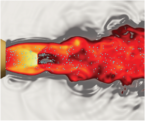
The particle-laden underexpanded jet configuration is shown in figure 1. A high-pressure gas is discharged from a sonic nozzle with an exit diameter  $D_e=2$ mm. As the gas exits the nozzle, it undergoes rapid expansion and acceleration, giving rise to supersonic flow downstream of the nozzle exit (refer to region 1 in the figure). Expansion waves initiated at the nozzle exit approach the jet boundary and subsequently reflect back towards the jet axis as weak compression waves (region 2 in the figure). When these waves coalesce, they form oblique shocks that meet at the jet axis. For nozzle pressure ratios
 $\eta _0\gtrapprox 4$ (see Franquet et al. Reference Franquet, Perrier, Gibout and Bruel2015), the oblique shocks no longer meet at the jet axis, and a Mach disk emerges (region 3 in the figure). A shear layer forms at the triple point, where the Mach disk and reflected shock merge. A comprehensive analysis and summary of underexpanded jets can be found in Franquet et al. (Reference Franquet, Perrier, Gibout and Bruel2015).
Numerical simulation of the underexpanded particle-laden jet showing the nozzle (blue), particles (white), local gas-phase Mach number (red/yellow) and density gradient (grey scale).

Particles of diameter  $d_p$ and density
 $\rho _p$ are injected upstream of the nozzle with a prescribed mass flow rate,
 $\dot {m}_p$. The mass loading is defined as the ratio of specific masses between the particles and the fluid, i.e.
 ${\varPhi _m} = \rho _p{\varPhi _v}/(\rho _e(1-{\varPhi _v}))$, where
 ${\varPhi _v}$ is the particle volume fraction and
 $\rho _e$ is the gas-phase density at the nozzle exit that can be determined from isentropic relations (see Appendix A.1). In this study, the mass loading is defined according to the ratio of mass flow rates,
 ${\varPhi _m}=\dot {m}_p/\dot {m}_f$, since it is easier to measure experimentally. With this, the average volume fraction at the exit of the nozzle can be determined according to
 ${\varPhi _v}={\varPhi _m} \rho _e/[\rho _p(1+{\varPhi _m}\rho _e/\rho _p)]$.
The velocity mismatch between the phases gives rise to a slip velocity that determines the particle Reynolds number  ${{Re}_p}$ and Mach number
 ${{M}_p}$ at the nozzle exit. The jet Reynolds number is defined as
 $Re=\rho _e U_e D_e/\mu$, where
 $\mu$ is the dynamic viscosity of the gas at the nozzle exit. The Stokes number is defined as
 $St=\tau _p/\tau _f$, where
 $\tau _p=\rho _p d_p^2/(18 \mu F_d)$ is the particle response time due to drag,
 $\tau _f=D_e/U_e$ is the characteristic fluid time scale based on the exit parameters and
 $F_d$ is the non-dimensional drag correlation of Osnes et al. (Reference Osnes, Vartdal, Khalloufi, Capecelatro and Balachandar2023) (see § 4.3) based on the exit conditions. The particle response time
 $\tau _p$ is sometimes given as the Stokes response time, i.e.
 $\tau _p^{St}=\rho _p d_p^2/(18\mu )$, so that acceleration due to drag is defined as
 $F_d(u_f-u_p)/\tau _p^{St}$. However, it is common to take the particle response time valid in the flow regime of interest, i.e.
 $\tau _p=\tau _p^{St}/F_d$ (see Fox, Laurent & Vié Reference Fox, Laurent and Vié2020). We chose the latter as it provides a Stokes number that is relevant for the flow conditions under consideration, as the physical response time of the particle deviates significantly from the Stokes response time owing to the large Reynolds numbers and Mach numbers.
A summary of the relevant parameters considered in this study are given in table 2. Experiments and simulations of unladen (single-phase) jets are also performed under the same conditions as the particle-laden configuration.
Summary of parameters considered in the current work. In each case, gas is discharged through a nozzle with diameter  $D_e=2$ mm into ambient conditions with an exit velocity
 $U_e=312$ m s
 $^{-1}$ and Mach number
 $M_e=1$.

3. Experimental set-up
3.1. High-speed jet facility
Figure 2 shows a schematic of the high-speed particle-laden jet facility at Johns Hopkins University. The facility consists of the air supply system and jet plenum, particle injection system and high-speed imaging system. Compressed air flows from a high-pressure tank into a jet manifold with three pressure regulators that allow for control of the stagnation pressure  $p_0$ and both
 $p_1$ and
 $p_2$, with the latter used for the particle injection system. To measure
 $p_0$, a pressure probe is inserted upstream of the nozzle exit in the constant-area section of the jet plenum, where the flow speed is subsonic. Due to the large diameter of the jet plenum (25.4 mm) and the low-speed flow, the difference between the static and stagnation pressure is negligible. For simplicity, we treat the measured static pressure as equivalent to the stagnation pressure. To control the nozzle pressure ratio
 $\eta _0$, the pressure regulator controlling the flow entering the jet plenum is set to the desired
 $p_0$. The facility is capable of achieving total pressure ratios within the range of
 $1.89 \leq \eta _0 \leq 6.86$, sufficient to study underexpanded and highly underexpanded jets. The flow is accelerated to sonic conditions using a commercial stainless-steel 303 conical nozzle (CCP-1, Ikeuchi, Inc.) with an exit diameter of
 $D_e = 2$ mm.
Schematic of the particle-laden underexpanded jet facility at Johns Hopkins University. Blue lines correspond the air flow and orange lines correspond to the particle flow.

3.2. Particle characteristics
Particles are injected into the flow stream by applying a pressure difference between  $p_1$ and
 $p_2$, which forces the stationary particles within the particle chamber to enter a feed tube that extends from the particle chamber to the end of the subsonic section of the jet plenum. Particles leave the chamber through an orifice diameter that is
 ${\sim }10d_p$ and enter a feed tube with an inner diameter of approximately 30 times the largest particle size in our experiments. Particles first travel into a section that is
 $219D_e$ long before turning
 $90^{\circ }$ to enter the jet centreline feed tube that is
 $330D_e$ long to ensure the two-phase flow becomes fully developed. Particles exit at the end of the feed tube
 $21D_e$ upstream of the nozzle exit. This allows for sufficient mixing between the particles and the subsonic gas before entering the converging section of the nozzle, where the flow is accelerated to sonic speeds at the nozzle exit. A large pressure gradient drives the flow of particles within the feeding tube. The Froude number in the feeder tube is
 $Fr=u_p^2/(gd_p)=O(10^5)$, where
 $u_p$ is the particle velocity and g is gravitational acceleration. Similarly, the Froude number based on the nozzle exit conditions is
 $Fr=U_e^2/(gd_p)=O(10^7)$, thus justifying negligible gravitational influence. Shadowgraph imaging shows the particles are symmetric about the axis. Particles are collected downstream of the nozzle using a cyclone separator (Oneida, Inc.). The particle mass flow rate is measured using a single-point load cell (PW4CM-2KG, HBM), positioned beneath the feeding chamber. The particle feeding rate was found to be insensitive to the height of the particle bed within the particle chamber. The mass flow rate of the particles is constant over time. This was cross-checked by manually measuring the mass flow rate of the particles at various time instances, showing a variation in the mass flow rate of less than 2 %. The electrical signal from the load cell is captured via a 16-bit data acquisition system (NI-9215, National Instruments), which is converted to a mass flow rate after obtaining a calibration relationship a priori. Further details on the mass flow rate calculation can be found in Kim et al. (Reference Kim, Ni, Capecelatro, Yao, Shallcross, Mehta and Rabinovitch2020).
The particles used in this study are clear poly(methyl methacrylate) acrylic microspheres (Cospheric LLC) with a density of  $\rho _p = 1211\,\mathrm {kg}\,\mathrm {m}^{-3}$. Three particle sizes were considered with mean diameters of
 $\bar {d}_p=29$,
 $42$ and
 $96\,\mathrm {\mu }$m, corresponding to Stokes numbers in the range
 $29< St<57$ (see table 2). The particle size distribution, shown in figure 4, was determined using laser diffraction acquired at NASA's Jet Propulsion Laboratory, California Institute of Technology, with deionized water as the dispersant. Measurements were carried out at brief, one second intervals over a minute, ensuring precise analysis.
3.3. High-speed imaging technique
Ultra-high-speed schlieren is used to visualize the gas-phase shock structures and particles. The optical set-up shown in figure 2 consists of a 100 W LED that passes through an iris to collimate the light, followed by a series of lenses that eventually collimate the light through the measurement plane. A horizontal knife edge was placed in front of the camera at the focal point to allow for the visualization of the changes in the density gradient in the vertical direction. In figure 2 a sample zoomed-in image is shown for case B3, where slight shock structures are visible near the jet boundary, clearly showing the effect of the knife edge.
In order to resolve the micron-sized particles in time and space, it was necessary to maximize the signal-to-noise ratio at the imaging sensor and minimize motion blur (Versluis Reference Versluis2013; Buchmann et al. Reference Buchmann, Cierpka, Kähler and Soria2014). The optimal frame rate for time-resolved imaging is defined as  $f=nU/S$, where
 $f$ is the frame rate,
 $n\geq 2$ is the number of samples to fulfil the sampling criterion,
 $U$ is the velocity scale and
 $S$ is a length scale. In this study, case A1 is expected to have the fastest particles due to the small size of
 $\bar {d}_p = 29\,\mathrm {\mu }$m. Assuming the particles reach velocities of
 $U_p = 200$ m s
 $^{-1}$ and knowing a priori that these particles move approximately 6 pixels frame to frame, results in a length scale
 $S = 210\,\mathrm {\mu }$m. Using these parameters, the optimal frame rate required for study is 1.87 MHz. Cases B1–B4 have larger particles that move slower, so this frame rate should suffice. Additionally, to avoid motion blur, the minimum exposure time is expressed as
 $\tau \leq d_p/U$, resulting in a required exposure time of
 $\tau \leq 145$ ns. To satisfy both
 $f$ and
 $\tau$ requirements, the Shimadzu HPV-X2 camera (FTCMOS2 sensor) was used, which enabled particle images to be acquired at 2 MHz at exposure times of 200 ns (camera limit). Although the required exposure time is lower than 200 ns, the particle images acquired for cases A1 and A2 were found to be sufficient for tracking. The resulting spatial resolutions are
 $17\,\mathrm {\mu }$m px
 $^{-1}$ for cases A1 and A2,
 $23\,\mathrm {\mu }$m px
 $^{-1}$ for cases B1 and B2 and
 $21\,\mathrm {\mu }$m px
 $^{-1}$ for cases B3 and B4, with an estimated depth of field of 1 mm. The resulting field of view is
 $5.6D_e$ in length and
 $3.5D_e$ in height, sufficient to capture the particle dynamics as particles pass through a pair of shock cells downstream of the nozzle. The camera outputs a total of 256 frames per run, necessitating approximately three to four experiments per case to ensure velocity statistics are adequately converged.
To track the particles, a Lagrangian particle tracking algorithm was applied to the acquired particle images. First, the particle positions were determined using weighted averaging and Gaussian fitting to determine particle centres, with the latter ensuring overlapping particles were also tracked. From the determined particle positions, particle trajectories were determined based on the nearest neighbour distance in the subsequent frames, followed by a convolution with a Gaussian smoothing kernel to estimate the particle velocities in each frame. Further details on this particle tracking algorithm can be found in Ouellette, Xu & Bodenschatz (Reference Ouellette, Xu and Bodenschatz2006) and Kelley & Ouellette (Reference Kelley and Ouellette2011).
4. Simulation details
4.1. Flow configuration
The numerical simulations were designed to match the experiments described in the previous section. A schematic view of the flow configuration is shown in figure 1. The computational domain is  $Lx \times Ly \times Lz = 30D_e \times 15D_e \times 15D_e$ discretized on a Cartesian mesh with
 $nx \times ny \times nz = 1201 \times 201 \times 201$ grid points. The mesh is uniform in the streamwise (
 $x$) direction with grid spacing
 $\Delta x=D_e/40$. Grid stretching is applied in the spanwise (
 $y$ and
 $z$) directions using the mapping proposed by Vishnampet, Bodony & Freund (Reference Vishnampet, Bodony and Freund2015) such that the grid spacing varies smoothly from
 $\Delta y_{min}=\Delta z_{min}=D_e/40$ at the centreline to
 $\Delta y_{max}=\Delta z_{max}=D_e/6$ at the lateral boundaries. The maximum point-to-point relative change in the grid spacing is
 ${<}4\,\%$. The minimum grid spacing is approximately three times smaller than the diameter of the largest particles considered. As shown in table 3, the maximum particle diameter is
 $150\,\mathrm {\mu }\mathrm {m}$.
Particle injection parameters. Velocities and diameters are sampled from normal and log-normal distributions, respectively. Additional parameters for each case are listed in table 2.

The nozzle extends  $4.35D_e$ into the domain. The inner contour (converging section) follows a hyperbolic tangent function with inner and outer diameters that match the experiment, ensuring the correct exit conditions (see Appendix A.1 for details). Particles are injected into the flow at the nozzle exit with a prescribed mass flow rate
 $\dot {m}_p$. Their velocity and diameter are randomly sampled from distributions informed by the experiments. More details on the velocity and size distribution can be found in § 4.5.
The numerical simulations are solved in a volume-filtered Eulerian–Lagrangian framework using a class of high-order, energy stable finite-difference operators (Shallcross, Fox & Capecelatro Reference Shallcross, Fox and Capecelatro2020; Capecelatro Reference Capecelatro2024). Here, individual particles are tracked in a Lagrangian frame, and the gas-phase equations are modified to incorporate volume displacement by particles and interphase momentum and energy exchange. Details on the governing equations and discretization are provided below.
4.2. Gas-phase description
The volume-filtered compressible Navier–Stokes equations describing the gas phase can be expressed compactly as
 \begin{equation} \frac{\partial \boldsymbol{Q}}{\partial t}+\frac{\partial}{\partial x_i} [\alpha(\boldsymbol{F}_i^I-\boldsymbol{F}_i^V)]=\boldsymbol{S}, \end{equation}
where  $\boldsymbol {Q} = [\alpha \rho, \alpha \rho u_i,\alpha \rho E]^{{\rm T}}$ is the vector of conserved variables,
 $\boldsymbol {F}_i^V$ and
 $\boldsymbol {F}_i^I$ are the viscous and inviscid fluxes and
 $\boldsymbol {S}$ contains source terms that account for two-way coupling with the particles, given by
 \begin{equation} \left.\begin{gathered} \boldsymbol{F}^I_i=\begin{bmatrix} \rho u_i \\ \rho u_1 u_i + p \delta_{i1} \\ \rho u_2 u_i + p \delta_{i2} \\ \rho u_3 u_i + p \delta_{i3} \\ u_i(\rho E + p) \end{bmatrix},\quad \boldsymbol{F}^V_i=\begin{bmatrix} 0 \\ \tau_{1i} \\ \tau_{2i} \\ \tau_{3i} \\ u_j \tau_{ij} - q_i \end{bmatrix},\\ \boldsymbol{S}=\begin{bmatrix} 0 \\ (p \delta_{i1}-\tau_{i1})\dfrac{\partial\alpha}{\partial x_i}+\mathcal{F}_1 \\ (p \delta_{i2}-\tau_{i2})\dfrac{\partial\alpha}{\partial x_i}+\mathcal{F}_2\\ (p \delta_{i3}-\tau_{i3})\dfrac{\partial\alpha}{\partial x_i}+\mathcal{F}_3\\ (\tau_{ij}-p \delta_{ij})\dfrac{\partial}{\partial x_i}(\alpha_p u_{p,j})+q_i \dfrac{\partial\alpha}{\partial x_i} \\ +\;u_{p,i}\mathcal{F}_i + \mathcal{Q} \end{bmatrix}. \end{gathered}\right\} \end{equation}
The conserved variables include the local gas-phase volume fraction  $\alpha$, density
 $\rho$, velocity
 $u_i$ (in direction
 $i$) and total energy
 $E$. In the source term,
 $\alpha _p=1-\alpha$ and
 $u_{p,i}$ are the volume fraction and velocity of the particle phase in an Eulerian frame, respectively, defined explicitly in § 4.4. The thermodynamic pressure is defined as
 $p = (\gamma -1)(\rho E - \rho u_i u_i/2)$, where
 $\gamma =1.4$ is the ratio of specific heats. The viscous stress tensor is given by
 \begin{equation} \tau_{ij} = \mu \left(\frac{\partial u_i}{\partial x_j} + \frac{\partial u_j}{\partial x_i}\right) + (\mu_b-2/3\mu) \frac{\partial u_k}{\partial x_k} \delta_{ij}, \end{equation}
where  $\delta _{ij}$ is the Dirac delta function and the bulk viscosity
 $\mu _b = 0.6\mu$ is chosen as a model for air (Sharma, Kumar & Pareek Reference Sharma, Kumar and Pareek2023). The shear viscosity varies with temperature based on a power law according to
 $\mu = \mu _{\infty }(T/T_{\infty })^{2/3}$, where
 $\mu _{\infty } = 1.8\times 10^{-5}\,\mathrm {Pa}\,\textrm {s}$ and
 $T_{\infty } = 298\,\mathrm {K}$ are the reference shear viscosity and temperature, respectively. Temperature is obtained from the ideal gas law,
 $T = p/(\rho R)$, where
 $R$ is the gas constant. The heat flux is defined as
 \begin{equation} q_i={-}\kappa\frac{\partial T}{\partial x_i}, \end{equation}
where  $\kappa$ is the thermal conductivity of the gas. Finally,
 $\mathcal {F}_i$ and
 $\mathcal {Q}$ are interphase momentum and heat exchange terms that will be defined in § 4.4.
Spatial derivatives are approximated using fourth-order, narrow-stencil finite-difference operators that satisfy the summation-by-parts (SBP) property (Strand Reference Strand1994). Kinetic energy preservation is achieved using a skew-symmetric-type splitting of the inviscid flux (Pirozzoli Reference Pirozzoli2011), extended to account for the effect of particles. Specifically, the convective fluxes appearing in (4.1) are expressed in split form as
 \begin{equation} \frac{\partial \alpha \rho u_i\varphi}{\partial x_i}=\frac{1}{2} \frac{\partial \alpha \rho u_i\varphi}{\partial x_i}+\frac{1}{2}\varphi \frac{\partial \alpha \rho u_i}{\partial x_i}+ \alpha \rho u_i\frac{\partial \varphi}{\partial x_i}, \end{equation}
where  $\varphi$ is a generic transported scalar that is unity for the continuity equation,
 $u_j$ for the momentum equation and
 $E+p/\rho$ for the total energy equation. This provides nonlinear stability at low Mach numbers.
To evaluate second and mixed derivatives, first derivative operators are applied consecutively, necessitating the use of artificial dissipation to damp the highest wavenumber components supported by the grid. High-order accurate SBP dissipation operators are used that provide artificial viscosity based on a sixth-order derivative (Mattsson, Svärd & Nordström Reference Mattsson, Svärd and Nordström2004). In addition, localized artificial diffusivity is used as a means of shock capturing following the formulation in Kawai, Shankar & Lele (Reference Kawai, Shankar and Lele2010). In this approach,  $\mu _b$ and
 $\kappa$ appearing in (4.3) and (4.4) are augmented based on a modified Ducros-type sensor. Full details on the shock capturing implementation are provided in Appendix A.3.
The SBP scheme is combined with the simultaneous approximation treatment (SAT) at the domain boundaries to facilitate an energy estimate (Carpenter, Gottlieb & Abarbenel Reference Carpenter, Gottlieb and Abarbenel1994; Nordström & Svärd Reference Nordström and Svärd2005). Non-reflecting characteristic boundary conditions (Svärd, Carpenter & Nordström Reference Svärd, Carpenter and Nordström2007) are enforced at each of the domain boundaries. No-slip, adiabatic boundary conditions are enforced at the surface of the nozzle via a ghost-point immersed boundary method (Chaudhuri, Hadjadj & Chinnayya Reference Chaudhuri, Hadjadj and Chinnayya2011; Khalloufi & Capecelatro Reference Khalloufi and Capecelatro2023). Further details on the nozzle profile and integration of the immersed boundary method in the SBP-SAT framework can be found in Appendix A.
The equations are advanced in time using a standard fourth-order Runge–Kutta scheme, resulting in the usual Courant–Friedrichs–Lewy (CFL) restrictions on the simulation time step  $\Delta t$ such that maximum CFL is 0.9. The CFL is taken as the maximum between the acoustic CFL,
 $\textrm {CFL}_a=\max (|\boldsymbol {u}|+c)\Delta t/\varDelta$ and the viscous CFL,
 $\textrm {CFL}_v = \max (2\mu,\mu _b,\kappa )\Delta t/\varDelta ^2$, where
 $\varDelta$ is the local grid spacing and
 $c=\sqrt {\gamma p/\rho }$ is the local sound speed. An additional time-step restriction is applied to ensure the source terms due to drag are resolved (Patel & Capecelatro Reference Patel and Capecelatro2022).
4.3. Particle-phase description
The particle equations of motion are given by
 \begin{equation} \frac{{\mathrm d}\kern0.7pt \boldsymbol{x}_p^{(i)}}{{\mathrm d}t} = \boldsymbol{v}_p^{(i)}, \end{equation}
and
 \begin{equation} m_p\frac{{\mathrm d}\boldsymbol{v}_p^{(i)}}{{\mathrm d}t}={V_p} \boldsymbol{\nabla}\boldsymbol{\cdot}(\boldsymbol{\tau} - p \boldsymbol{I}) + {{\boldsymbol{F}}_{drag}^{(i)}} + {{\boldsymbol{F}}_{lift}^{(i)}} + {{\boldsymbol{F}}_{am}^{(i)}}, \end{equation}
where  $\boldsymbol {I}$ is the identity tensor,
 $\boldsymbol {x}_p^{(i)}=(x_p^{(i)},y_p^{(i)},z_p^{(i)})$ and
 $\boldsymbol {v}_p^{(i)}=(v_{p,x}^{(i)},v_{p,y}^{(i)},v_{p,z}^{(i)})$ are the position and velocity of particle
 $i$, respectively,
 $m_p$ is the mass of the particle and
 $V_p$ is its volume. Also,
 ${\boldsymbol {F}}_{drag}^{(i)}$,
 ${\boldsymbol {F}}_{lift}^{(i)}$ and
 ${\boldsymbol {F}}_{am}^{(i)}$ are the force contributions due to drag, lift and added mass, respectively.
The unsteady aerodynamic forces acting on a particle (i.e. the pressure gradient and added mass) are typically neglected in low-speed, gas–solid flows due to the high density ratio. However, under sufficient gas-phase acceleration, such as in flows with shocks, the unsteady contributions can dominate (Parmar, Haselbacher & Balachandar Reference Parmar, Haselbacher and Balachandar2009; Ling, Haselbacher & Balachandar Reference Ling, Haselbacher and Balachandar2011) and are thus considered here. Due to the low volume fractions considered, inter-particle collisions are neglected.
The quasi-steady drag force is given by
 \begin{equation} \frac{{\boldsymbol{F}}_{drag}^{(i)}}{m_p}=\frac{1}{\tau_p}(\boldsymbol{u}-{\boldsymbol{v}}_p^{(i)}), \end{equation}
where  $\tau _p=\rho _p d_p^2$/
 $(18\mu F_d)$ is the particle response time due to drag and
 $F_d=F_d(\alpha _p,Re_p, M_p)$ is the non-dimensional drag correlation of Osnes et al. (Reference Osnes, Vartdal, Khalloufi, Capecelatro and Balachandar2023). Here,
 $Re_p=\rho |\boldsymbol {u}-\boldsymbol {v}_p^{(i)}|d_p$/
 $\mu$ is the particle Reynolds number and
 $M_p=|\boldsymbol {u}-\boldsymbol {v}_p^{(i)}|$/
 $c$ is the particle Mach number.
The Saffman lift force is modelled according to (McLaughlin Reference McLaughlin1991)
 \begin{equation} {{\boldsymbol{F}}_{lift}^{(i)}} = \frac{9.69 \sqrt{\rho \mu}}{{\rm \pi} \rho_p d_p} \frac{(\boldsymbol{u}-\boldsymbol{v}^{(i)}_p) \times \boldsymbol{\omega}}{\sqrt{|\boldsymbol{\omega}|}}, \end{equation}
where  $\boldsymbol {\omega }$ is the gas-phase vorticity.
Following the formulation proposed by Parmar, Haselbacher & Balachandar (Reference Parmar, Haselbacher and Balachandar2010), added mass is expressed as
 \begin{equation} \boldsymbol{F}_{am}^{(i)} = V_pC_M(M_p, \alpha_p)\left[\frac{{\rm D}(\rho \boldsymbol{u})}{{\rm D}t}- \frac{{\rm d}(\rho_p \boldsymbol{v}_p^{(i)})}{{\rm d}t}\right], \end{equation}
where  $C_M = C_{M,0}\eta _1(M_p)\eta _2(\alpha _p)$ is the added-mass coefficient (Ling et al. Reference Ling, Haselbacher and Balachandar2011) and
 $C_{M,0}=0.5$ is the value in the zero Mach number and zero volume fraction limit. The Mach number correction of Parmar, Haselbacher & Balachandar (Reference Parmar, Haselbacher and Balachandar2008) and volume fraction correction of Sangani, Zhang & Prosperetti (Reference Sangani, Zhang and Prosperetti1991) are employed, expressed as
 \begin{equation} {} \eta_1(M_p)= \begin{cases} 1 + 1.8 M_p + 7.6M^4_p & \text{if } M_p < 0.6,\\ 2.633, & \text{otherwise} \end{cases}\quad\text{and}\quad \eta_2(\alpha_p) = \frac{1 + 2\alpha_p}{1-\alpha_p}. \end{equation}
The evolution of particle temperature is given by
 \begin{equation} m_p C_{p,p} \frac{{\mathrm d}T^{(i)}_p}{{\mathrm d}t} = {q}^{(i)}_{inter}, \end{equation}
where  $C_{p,p}$ is heat capacity of the particle,
 $T^{(i)}_p$ is its temperature and
 $q^{(i)}_{inter}$ is the interphase heat exchange given by
 \begin{equation} q^{(i)}_{inter} = \frac{6V_p\kappa {Nu}}{d_p^2}(T-T^{(i)}_p), \end{equation}
where  ${Nu}$ is the Nusselt number that is modelled using the correlation of Gunn (Reference Gunn1978).
Particles are advanced in time simultaneously with the fluid via a fourth-order Runge–Kutta scheme. Special care needs to be taken when evaluating fluid quantities appearing in (4.8)–(4.13) at the location of the particle, namely  $\alpha$,
 $\rho$,
 $\boldsymbol {u}$,
 $\mu$,
 $\boldsymbol {\nabla }\boldsymbol {\cdot }(\boldsymbol {\tau } - p \boldsymbol {I})$,
 $\boldsymbol {\omega }$ and
 $T$, especially near shocks where the flow is nearly discontinuous (see figure 3). These details will be given in § 4.4.
Schematic of a classical interpolation scheme for a particle in the vicinity of a shock.

4.4. Two-way coupling
Particle information (drag, heat exchange, volume fraction, etc.) is projected to the Eulerian grid using the two-step filtering approach proposed by Capecelatro & Desjardins (Reference Capecelatro and Desjardins2013). The gas-phase volume fraction is computed according to
 \begin{equation} {} \alpha(\boldsymbol{x},t) =1- \sum_{1}^{N_p}\mathcal{G}\Big(|\boldsymbol{x}-\boldsymbol{x}^{(i)}_p|\Big) V_p, \end{equation}
where  $\mathcal {G}$ is a Gaussian filter kernel with a characteristic length
 $\delta _f=4\bar {d}_p$ taken to be the full width at half-maximum,
 $N_p$ is the total number of particles and
 $\boldsymbol {x}$ is the position on the Eulerian grid. Interphase momentum exchange appearing in the source term of (4.1) is given by
 \begin{equation} \boldsymbol{\mathcal{F}} ={-} \sum_{i=1}^{N_p} \mathcal{G}\Big(|\boldsymbol{x}-\boldsymbol{x}_p^{(i)}|\Big) \Big(\boldsymbol{F}_{drag}^{(i)} + \boldsymbol{F}_{lift}^{(i)} + \boldsymbol{F}_{am}^{(i)}\Big). \end{equation}
Similarly, the work done by drag appearing in the energy equation is expressed as
 \begin{equation} \boldsymbol{u}_p \boldsymbol{\cdot} \boldsymbol{\mathcal{F}} ={-} \sum_{i=1}^{N_p} \mathcal{G}\Big({|\boldsymbol{x}-\boldsymbol{x}_p^{(i)}|}\Big)\Big(\boldsymbol{F}_{drag}^{(i)} + \boldsymbol{F}_{lift}^{(i)} + \boldsymbol{F}_{am}^{(i)}\Big) \boldsymbol{\cdot} \boldsymbol{v}_p^{(i)}, \end{equation}
and the interphase heat exchange term is given by
 \begin{equation} \mathcal{Q} ={-} \sum_{i=1}^{N_p} \mathcal{G}\Big(|\boldsymbol{x}-\boldsymbol{x}_p^{(i)}|\Big){q}_{inter}^{(i)}. \end{equation}
The models employed in the particle equation of motion (4.7) were formulated using correlations reliant on ‘far-field’ fluid quantities, such as velocity, temperature and volume fraction that remain unaffected by the presence of the particle. In order for these models to be applicable in a two-way coupled simulation, the self-induced disturbance must be removed. This has been an active area of research in recent years (e.g. Horwitz & Mani Reference Horwitz and Mani2016, Reference Horwitz and Mani2018; Balachandar, Liu & Lakhote Reference Balachandar, Liu and Lakhote2019; Liu, Lakhote & Balachandar Reference Liu, Lakhote and Balachandar2019; Evrard, Denner & van Wachem Reference Evrard, Denner and van Wachem2020; Pakseresht, Esmaily & Apte Reference Pakseresht, Esmaily and Apte2020; Pakseresht & Apte Reference Pakseresht and Apte2021). However, models have not yet been extended to compressible flows. Various interpolation techniques have been proposed for particles in the vicinity of shocks (Jacobs & Don Reference Jacobs and Don2009; Kozak et al. Reference Kozak, Dammati, Bravo, Hamlington and Poludnenko2020), although their application to finite size particles necessitating corrections for self-induced disturbances has not yet been explored. Recently, Yang et al. (Reference Yang, Li, Liu, Sun, Yang, Wang, Wang and Li2023) proposed a weighted average-based interpolation scheme with weights biased away from the particle centre to interpolate far-field conditions. This was reported to restore the undisturbed quantities.
A simple approach to remove the effect of self-induced disturbances is to filter the fluid field prior to interpolation (Evrard et al. Reference Evrard, Denner and van Wachem2020). A similar strategy is followed in this work. Any gas-phase quantity,  ${\zeta }(\boldsymbol {x},t)$, appearing in (4.8)–(4.13) (i.e.
 $\alpha$,
 $\rho$,
 $\boldsymbol {u}$,
 $\mu$,
 $\boldsymbol {\omega }$ and
 $T$) is evaluated at the particle position via convolution with a Gaussian filter according to
 \begin{equation} \tilde{\zeta}[\boldsymbol{x}_p^{(i)}(t)] = \int_V{\mathcal{G}\Big(|\boldsymbol{x}-\boldsymbol{x}_p^{(i)}|\Big){\zeta}(\boldsymbol{x},t)\,\mathrm{d}V}. \end{equation}
However, a direct application of (4.18) can be computationally expensive as it requires each particle to loop through (potentially) many surrounding grid points (Capecelatro & Desjardins Reference Capecelatro and Desjardins2013). Instead, this is performed in two steps according to
 \begin{equation} \tilde{\zeta}[\boldsymbol{x}_p^{(i)}(t)] \approx \sum_{k=1}^{n}\mathcal{W} \Big(|\boldsymbol{x}-\boldsymbol{x}_p^{(i)}|\Big) \bar{\zeta}(\boldsymbol{x},t)\,\mathrm{d}V\quad\text{with}\ \bar{\zeta}(\boldsymbol{x}, t) = \zeta(\boldsymbol{x}, t) * \mathcal{G}, \end{equation}
where  $\mathcal {W}$ corresponds to weights of a tri-linear interpolation scheme that is localized to the
 $n$ nearest grid cells of particle
 $i$. The
 $\overline {({\cdot })}$ notation denotes a filtered quantity on the grid that can be solved efficiently via an alternating-direct-implicit scheme. The efficacy of the proposed interpolation scheme is demonstrated for a single particle passing through a standing shock in Appendix A. It was found that interpolating the gas-phase stress tensor,
 $\boldsymbol {\nabla }\boldsymbol {\cdot } (\boldsymbol {\tau } - p \boldsymbol {I})$, without filtering is necessary to avoid excessive smearing of discontinuities in the presence of shocks (see figure 3) and give reasonable estimate of the undisturbed gradients.
4.5. Particle injection
One challenge in replicating the experimental conditions is the difficulty in obtaining optical access near the nozzle exit. Although the mass loading is well characterized, precise three-dimensional particle positions and velocities are not known. To address this, particles are randomly placed at the nozzle exit while adhering to the known mass loading. Their velocities are sampled from distribution functions designed to ensure statistical agreement within the first  $D_e/4$ of the nozzle. Further details are provided below.
Particles are seeded in the computational domain at the nozzle exit after the gas phase reaches a statistically stationary state. The number of particles injected per timestep,  $N(t)$, is determined from the experimentally measured mass flow rate according to
 \begin{equation} \dot m_p = \sum_{i=1}^{N(t)}\frac{{\rm \pi} {d_p^{(i)}}^3 \rho_p}{6\Delta t}. \end{equation}
Particles are injected uniformly random throughout the cross-section of the nozzle exit plane according to
 \begin{equation} x_p^{(i)} = 0,\quad y_p^{(i)} = \frac{D_e}{2}\sqrt{\mathcal{R}} \cos(\mathcal{R}2{\rm \pi}),\quad z_p^{(i)} = \frac{D_e}{2}\sqrt{\mathcal{R}} \sin(\mathcal{R}2{\rm \pi}), \end{equation}
where  $\mathcal {R}\in [0,1]$ is a uniform random real number. Particle diameters are sampled randomly from log-normal distributions,
 $d_p\sim \textrm {Log-normal}(\bar {d}_p,\sigma _d)$, where the mean (
 $\bar {d}_p$) and standard deviation (
 $\sigma _d$) are determined from particle size distributions obtained experimentally (see figure 4). The values for each case are reported in table 3.
Particle size distribution. Raw data:  $\bar {d}_p=29.6\,\mathrm {\mu }$m (
 $\bullet$, purple),
 $\bar {d}_p=42\,\mathrm {\mu }$m (
 $\bullet$, blue)
 $\bar {d}_p=96\,\mathrm {\mu }$m (
 $\bullet$, green). Lines are fitted log-normal distributions using the parameters listed in table 3.

Similarly, newly seeded particles are assigned velocities that are randomly sampled from normal distributions  $\mathcal {N}(\boldsymbol {U}_p,\sigma _{\boldsymbol {U}})$ fit to the experimental data with mean
 $\boldsymbol {U}_p=(U_p,V_p)$ and standard deviation
 $\sigma _{\boldsymbol {U}}=(\sigma _U,\sigma _V)$. Here, the streamwise particle velocities are sampled from
 $v_{p,x}\sim \mathcal {N}(U_p,\sigma _{U})$ and due to axial symmetry the spanwise velocities are sampled from
 $v_{p,y}\sim \mathcal {N}(V_p,\sigma _{V})$ and
 $v_{p,z}\sim \mathcal {N}(V_p,\sigma _{V})$. Probability density functions (PDFs) of the streamwise and spanwise particle velocities are collected experimentally near the nozzle exit within a window
 $0\le x/D_e\le 0.25$ (see figure 5). The velocity distributions from the experiments were approximated as Gaussian due to its simplicity and reproducibility. The parameters used in the simulations are chosen so that the mean and standard deviations match within this region. The values are given in table 3.
Particle velocity distributions near the nozzle exit ( $0\le x/D_e\le 0.25$). (a,b) Case A1, (c,d) case A2, (e,f) case B1, (g,h) case B2, (i,j) case B3, (k,l) case B4. Experiments: streamwise velocity (
 $\blacksquare$, red) and spanwise velocity (
 $\blacksquare$, blue). Simulations: streamwise velocity (
 $\blacksquare$, translucent red) and spanwise velocity (
 $\blacksquare$, translucent blue).

5. Results and discussion
5.1. Single-phase jet
In this section, comparisons are made between the experiments and simulations of the single-phase jet. Shock structures are visualized in the experiments using an inline-type schlieren imaging system. Filters and converging lenses are employed to generate a spatially filtered collimated beam. At the focal point of the beam, a horizontal knife-edge cutoff is used to enhance the density gradient in the flow. The ensemble average is calculated using 256 instantaneous images in both the experiments and simulations, corresponding to  $138\,\mathrm {\mu }$s of data. The numerical schlieren is produced by first integrating the vertical density gradient along the field of view (
 $z$-direction),
 $\psi (x,y)=\int \partial \rho /\partial y\,\textrm {d}z$, then applying the scaling proposed by (Quirk Reference Quirk1997)
 \begin{equation} \xi = \exp({-}k \psi_s)\quad\text{with}\ \psi_s = \frac{\psi-k_0(\partial \rho/\partial y)_{max}}{k_1(\partial \rho/\partial y)_{max}- k_0(\partial \rho/\partial y)_{max}}, \end{equation}
where  $k=5$,
 $k_0=-0.001$ and
 $k_1 = 0.05$.
Figure 6 shows schlieren images produced experimentally and numerically for nozzle pressure ratios  $\eta _0 = 3.40$ and
 $6.46$. Regions of expansion fans, compression waves, oblique shocks and their spatial repetition are evident. At a pressure ratio
 $\eta _0 = 3.40$, the jet has a diamond shock structure with merged oblique shocks at the centreline near
 $x/D_e = 1.1$. Increasing the pressure ratio to
 $\eta _0 = 6.46$ causes the Mach disk to grow in size and move further downstream. The new shock structure resembles a barrel shock cell. The numerical schlieren shows overall good agreement with experiments. Some discrepancy can be observed at the lower pressure ratio of
 $\eta _0=3.4$ (figure 6a,c) downstream of the first Mach disk.
Ensemble-averaged schlieren obtained from experiments (a,b) and simulations using the scaling given in (5.1) (c,d) for  $\eta _0 = 3.40$ (a,c) and
 $\eta _0 = 6.46$ (b,d).

The normalized Mach disk location is extracted from averaged schlieren images and reported for a wide range of pressure ratios in figure 7. The validation is extended by comparing against previous works in the literature, including the empirical correlation proposed by Crist, Glass & Sherman (Reference Crist, Glass and Sherman1966), given by
 \begin{equation} \frac{L_{MD}}{D_{e}} = \sqrt{\frac{\eta_0}{2.4}}. \end{equation}
Position of the Mach disk as a function of the total pressure ratio for single-phase flow. Current experiments ( $\blacksquare$, purple) and simulations (
 $\square$, purple), Ashkenas & Sherman (Reference Ashkenas and Sherman1965) (
 $\times$), Crist et al. (Reference Crist, Glass and Sherman1966) (
 , six star open), Hatanaka & Saito (Reference Hatanaka and Saito2012) (
 $\lozenge$), Tabei, Shirai & Takakusagi (Reference Tabei, Shirai and Takakusagi1992) (
 $\square$), Sommerfeld (Reference Sommerfeld1994) (
 $\triangle$), Gibbings, Ingham & Johnson (Reference Gibbings, Ingham and Johnson1972) (
 $+$), Addy (Reference Addy1981) (), correlation by Crist et al. (Reference Crist, Glass and Sherman1966) (5.2) (—–).

Both experiments and simulations show good agreement with the correlation and previous experiments from the literature. Simulations were conducted at elevated pressure ratios ( $\eta _0=[8, 10, 30]$) for further validation. Overall, excellent agreement is observed. It should be noted that significant variation has previously been reported at pressure ratios below
 $\eta _0<5$ (Franquet et al. Reference Franquet, Perrier, Gibout and Bruel2015). Consequently, (5.2) is less valid at such low pressure ratios, although good agreement is still observed with the present experiments and simulations. This might also explain the discrepancy in the shock structures observed in figure 6 at
 $\eta _0=3.4$.
Figure 8 shows the average centreline Mach number obtained from the simulation for  $\eta _0=3.4$. Comparisons are made against experiments by Henderson, Bridges & Wernet (Reference Henderson, Bridges and Wernet2005) and a solution obtained from the method of characteristics (MOC) (Owen & Thornhill Reference Owen and Thornhill1948). The MOC solution assumes steady supersonic inviscid flow with rotational symmetry and
 $\eta _0 = \infty$. Both simulations and experiments agree well with the MOC solution in the near-field region up to the first Mach disk. Beyond this point, the MOC solution is no longer valid due to the presence of discontinuities.
Centreline Mach number obtained from experiments of a single-phase sonic jet from Henderson et al. (Reference Henderson, Bridges and Wernet2005) ( $\triangle$), MOC solution (Owen & Thornhill Reference Owen and Thornhill1948) (- - -) and numerical simulations performed in the present study (——) with
 $\eta _0=3.40$.

While the location of Mach diamonds predicted by the simulation are in good agreement with the experiment shown in figure 8, the local Mach number is over-estimated by  $\approx$20 %. The discrepancy with the experiment can be attributed to the non-negligible Stokes number associated with the seeded particles used with the experimental particle image velocimetry (PIV) system (
 $0.6\,\mathrm {\mu } \textrm {m}$ diameter particles were used). Finite size particles used for optical flow measurements lag sudden changes in the gas phase, especially through discontinuities such as shocks, resulting in an under-prediction in the peak Mach number. Henderson et al. (Reference Henderson, Bridges and Wernet2005) estimate
 $0.04D_e-0.12D_e$ of particle lag downstream of the Mach disk, which is orders of magnitude larger than the shock thickness. Similar discrepancies in the centreline Mach number profile between simulations and experiments have previously been reported (e.g. Saddington, Lawson & Knowles Reference Saddington, Lawson and Knowles2004; Gojon & Bogey Reference Gojon and Bogey2017).
5.2. Two-phase jet: particle dynamics
Particle velocity statistics are reported at different downstream locations from  $0 \leq x/D_e \leq 4$ divided into windows with width of
 $D_e$. Simulation results are collected at the same frame rate as the experiments, corresponding to 256 snapshots taken in a
 $130\,\mathrm {\mu }$s time window. Figure 9 shows the PDFs for the streamwise and spanwise particle velocities for case A2 (
 ${\varPhi _m}= 0.37$,
 $\bar {d}_p = 29\,\mathrm {\mu }$m). Particles are injected into a rapidly accelerating gas phase, causing them to gain momentum through drag. This is evident in figure 9 as the particle streamwise velocity increases from the mean of
 $\approx$175 to
 $\approx$220 m s
 $^{-1}$. Note that the shape of the streamwise velocity distribution (red) also changes with the streamwise distance. As particles travel downstream, the spanwise velocity distribution remains Gaussian (with zero mean) with marginal increase in variance owing to rotational symmetry of the flow.
Velocity PDFs for case A2 measured in the region (a,b)  $0\leq x/D_e <1$, (c,d)
 $1 \leq x/D_e <2$, (e,f)
 $2 \leq x/D_e <3$ and (g,h)
 $3 \leq x/D_e <4$. Experiments: streamwise velocity (
 $\blacksquare$, red) and spanwise velocity (
 $\blacksquare$, blue). Simulations: streamwise velocity (
 $\blacksquare$, translucent red) and spanwise velocity (
 $\blacksquare$, translucent blue). Mean injection velocity (- - -).

On the other hand, the streamwise velocity distribution exhibits skewness which is captured by both simulations and experiments. However, the skewness is more pronounced for the experiments. These distributions suggest a higher number density for the faster-moving particles, especially for the simulations. The ability to capture this occurrence is important for applications such as plume surface interactions during landing where these fastest-moving particles are the ones that could cause damage to the landing platform. The mean and variance of particle velocities with respect to streamwise distance are shown in Appendix A.4.
When the particle size and mass loading are increased (i.e. from case A2 to case B4), particles do not experience as significant of an acceleration. This is attributed to the higher Stokes number compared with case A2 resulting in increased lag. It can also be observed that the particles accelerate the most in the vicinity of the nozzle exit ( $0 \leq x/D_e \leq 2$) where the gas-phase acceleration is significantly higher. Similar to case A2, there is an overall good agreement in the mean particle velocity observed between simulations and experiments. However, the streamwise velocity variance is slightly underpredicted at
 $x/D_e>2$. It is interesting to note that, in case A2 (involving smaller particles), the simulations are capable of capturing the skewness in the PDF observed experimentally. In case B4 (with larger particles and higher
 $\eta _0$), the skewness in the experiments is less pronounced and is completely absent in the simulations and is consistent with the velocity distributions observed in the other cases considered (see Appendix A.4). These results also reveal that there is a significant momentum exchange between the phases, especially in the initial shock cells.
Figures 9, 10 and in Appendix A.4 reveal the spanwise velocity statistics remain relatively unchanged within the first four diameters downstream of the nozzle, even for the smallest particles considered. It can also be seen from figure 5 that the width of the spanwise velocity PDF is similar between cases A2 and B2, which have different sized particles. This is interesting to note, as previous works have observed stronger modulation of the shock structure for smaller particles, suggesting this is due to increased radial spread at lower Stokes numbers (Sommerfeld Reference Sommerfeld1994), although these results suggest the difference in radial spread is not substantial.
Velocity PDFs for case B4 measured in the region (a,b)  $0\leq x/D_e <1$, (c,d)
 $1 \leq x/D_e <2$, (e,f)
 $2 \leq x/D_e <3$ and (g,h)
 $3 \leq x/D_e <4$. Experiments: streamwise velocity (
 $\blacksquare$, red) and spanwise velocity (
 $\blacksquare$, blue). Simulations: streamwise velocity (
 $\blacksquare$, translucent red) and spanwise velocity (
 $\blacksquare$, translucent blue). Mean injection velocity (- - -).

Figure 11 presents the streamwise centreline velocities of both phases for two different nozzle pressure ratios, alongside the corresponding single-phase velocity for comparison. Due to the discrete treatment of the particle phase, the particle centreline velocity is calculated based on a cylindrical volume with a radius of 0.1 $D_e$, although the results were found to be insensitive to the specific choice in radius.
Time-averaged centreline velocities. Panel (a) shows  $\eta _0=3.4$; case A1 (—–, grey) and case A2 (—–, black). Panel (b) shows
 $\eta _0=6.46$; case B1 (—–, grey) and case B4 (—–, black), dashed lines represent corresponding particle velocities from the simulations. Corresponding single-phase velocity (—–, blue). Symbols represent time-averaged particle-phase velocities obtained from the experiments. Velocities are normalized by the gas-phase nozzle exit velocity
 $U_e$.

Similar to the observations in figures 9 and 10, the time-averaged particle velocities obtained from the simulations exhibit excellent agreement with the experiments. Due to their high inertia, particles exhibit near-ballistic behaviour. Their velocities increase monotonically, with maximum acceleration occurring within  $x/D_e < 2$, where the maximum gas-phase acceleration is observed. Particles experience a notable lag relative to the gas phase, leading to a high slip velocity across most of the streamwise distance. The centreline gas-phase velocities indicate stronger two-way coupling at higher pressure ratio, with greater deviations from the single-phase profile as mass loading and downstream distance increase. Compared with the single-phase flow at approximately
 $x/D_e \approx 5$, the gas-phase velocity completely diverges from phase alignment for the higher pressure ratio with the greatest mass loading (case B4). The maximum change in gas-phase velocity compared with the single-phase case occurs downstream of where the maximum interphase slip velocity is observed. This suggests that there is finite time (and distance) over which momentum and energy transfer accumulates until notable flow modulation is observed.
5.3. Changes in Mach disk characteristics
The focus of this study lies in examining the movement of the Mach disk location due to the presence of particles. As mentioned in § 1, the introduction of particles leads to an upstream movement of the Mach disk toward the nozzle exit. In this section, we demonstrate how the Mach disk and surrounding gas structures undergo modifications due to two-way coupling by particles.
Figure 12 shows experimental snapshots of a flow with soda lime glass beads with a mean particle diameter of  $\bar {d}_p = 140\,\mathrm {\mu }$m and
 ${\varPhi _m} = 0.37$, visualized by placing a vertical knife edge at the focal plane to enhance density gradients in the horizontal direction. Figures 12 and 13 are shown for qualitative purposes. These cases were omitted from table 2 because the larger particles obscure the gas-phase discontinuities, making it difficult to quantify the Mach disk shift. Figure 12(a) shows the unladen jet at
 $\eta _0 = 4.42$, representing a highly underexpanded jet with a large Mach disk downstream of the nozzle. The image shows a few particles entering the field of view, which results in the structure of the jet being significantly affected as evident in figure 12(b), where the shock cell and Mach disk have moved closer towards the nozzle, and the oblique shocks appear more distorted. However, the shock cell remains intact. In figure 12(c), a pair of particles interact with the Mach disk, distorting a portion of the Mach disk, yet the shock cell remains intact. However, in figure 12(d), a particle passing through the jet centreline results in significant distortion of the shock cell and Mach disk. Despite only a few particles entering the field of view, two particles are enough to fully distort the Mach disk and surrounding shock structures. It is important to note that the Mach disk structure is three-dimensional, and therefore, the distortions are also three-dimensional. However, the conclusions drawn from these results are based on the projected two-dimensional measurements.
Instantaneous experimental snapshots of (a) the unladen jet at  $\eta _0 = 4.42$ and (b) observations of two-way coupling using particles with a mean diameter of
 $\bar {d}_p = 140\,\mathrm {\mu }$m,
 $\eta _0 = 4.42$ and
 $\varPhi _m = 0.37$. The particles and the gas flow from left to right and were taken at (b)
 $t = 79\,\mathrm {\mu }$s, (c)
 $t = 84\,\mathrm {\mu }$s, (d)
 $t = 89\,\mathrm {\mu }$s. The scale bar is 1 mm in length.

Experimental images showing comparisons between the (a) single-phase jet and particle-laden case with  $\bar {d}_p = 140\,\mathrm {\mu }$m particles and
 $\eta _0 = 3.40$ with (b)
 ${\varPhi _m} = 0.80$, (c)
 ${\varPhi _m} = 1.73$ and (d)
 ${\varPhi _m} = 2.26$. The scale bar is 1 mm for all is 1 mm in length.

In addition to the modification of the portions of the Mach disk, the presence of particles in the high-speed and accelerating flow results in the generation of three-dimensional bow shocks upstream of individual particles, as shown in figure 12(b). The emergence of bow shocks is due to the large slip Mach number  $M_p > 1$. These structures manifest upstream of the Mach disk, within the supersonic flow regime, and dissipate downstream of the Mach disk where the flow is subsonic. Farther downstream of the shock cell, the flow accelerates to supersonic speeds, and bow shocks emerge once again around the particles. The presence of bow shocks could potentially alter the surrounding flow properties further, as these structures extend to the jet boundary, as seen for some of the particles. In figure 12(c), a reflected shock is clearly visible above the pair of particles interacting with the Mach disk, which could be emanating from near the nozzle region where several particles are located. In addition, the time sequence shows the interaction of bow shocks between neighbouring particles near the nozzle exit. This was previously observed and analysed in experimental and numerical work on shock–shock interaction in the two-particle system by Laurence, Parziale & Deiterding (Reference Laurence, Parziale and Deiterding2012). Figure 12(d) also shows an instance of a bow shock interacting with the distorted Mach disk.
The distortion of the Mach disk and shock cell at low mass loadings clearly show the strength of the two-way coupling. When  ${\varPhi _m}$ becomes larger, the momentum of the flow is further reduced due to drag by the particles. Figure 13 shows instantaneous experimental images with
 $\eta _0 = 3.40$ and particles of
 $\bar {d}_p = 140\,\mathrm {\mu }$m. Figure 13(a) shows the single-phase jet, with a small Mach disk diameter and visible oblique and reflected shocks. When particles are present at
 ${\varPhi _m} = 0.80$, a shock cell is no longer visible, and the Mach disk appears to be broken down, a similar behaviour as in figure 12. As the mass loading increases beyond
 ${\varPhi _m} > 1$, both shock cell and Mach disk completely disappear, as seen in figure 13(c,d). The only remaining shock structures in the flow are the bow shocks around particles, which wrap around the particles at
 ${\varPhi _m} < 1$ (see figure 13b) and become a curtain of shock structures as the mass loading is increased (see figure 13c,d).
To quantify these shock structure changes, the location of the Mach disk is extracted from both experiments and simulations. This is performed by averaging every image together within each experimental and simulation run (a total of  $130\,\mathrm {\mu }$s with 256 frames). After obtaining the ensemble average image in the experiments, the background (an image in which the disk was filtered out) is subtracted, and a low-pass Fast Fourier Transform (FFT) filter is applied to enhance the signal-to-noise ratio of the shock structure (Shapiro & Stockman Reference Shapiro and Stockman2001). Similar to Shekhtman et al. (Reference Shekhtman, Yu, Mustafa, Parziale and Austin2021), the Gaussian peak finding algorithm from O'Haver (Reference O'Haver1997) is then used to determine the locations of the Mach disk and oblique shock waves that shoulder it. The endpoints of the Mach disk were determined by intersections of linear fits for the Mach disk and oblique shocks. The error analysis for the Mach disk (the upper and lower intersection points of the disk with an oblique shock) was performed by using the confidence intervals for lines fitted on signal peaks. This error is propagated along with the standard deviation obtained from multiple runs and is converted to real units using the corresponding spatial resolution for each case studied. Such treatment is not required in the simulations since the particles can be easily decoupled from the gas phase during post-processing. The Mach disk location is extracted in this manner for all of the runs for each case. After obtaining the Mach disk location from experiments and simulations, the relative shift in the Mach disk location as a function of mass loading is computed and shown in figure 14.
Relative shift in the Mach disk location as a function of mass loading. Experiments in the present study:  $\eta _0= 3.4$,
 $\bar {d}_p = 29\,\mathrm {\mu }$m (
 $\blacktriangle$, purple),
 $\eta _0= 6.46$,
 $\bar {d}_p = 42\,\mathrm {\mu }$m and
 $96\,\mathrm {\mu }$m (
 $\blacksquare$, purple). Simulations:
 $\eta _0= 3.4$,
 $\bar {d}_p = 29\,\mathrm {\mu }$m (
 $\triangle$, purple),
 $\eta _0= 6.46$,
 $\bar {d}_p = 42\,\mathrm {\mu }$m and
 $96\,\mathrm {\mu }$m (
 $\square$, purple). Experiments by Sommerfeld (Reference Sommerfeld1994) with
 $\textrm {NPR}\approx 30$ (
 $\bullet$, purple). Jain et al. (Reference Jain, Chen, Panerai and Villafañe Roca2024) with
 $\eta _0= 3.46\unicode{x2013} 6.23$,
 $\bar {d}_p = 116\,\mathrm {\mu }$m (
 $\blacktriangleright$, purple), simulations from Carcano et al. (Reference Carcano, Bonaventura, Esposti and Neri2013) (
 , Six Star Open, purple), experiments by Lewis & Carlson (Reference Lewis and Carlson1964):
 ${M}_e=2.905$ (
 , green),
 ${M}_e=1.75$ (
 , Six Star Open, blue). Solid lines correspond to the empirical correlation (5.3). Larger symbols indicate bigger particles.

Experiments by Lewis & Carlson (Reference Lewis and Carlson1964) (also shown in figure 14) were performed at supersonic exit Mach numbers for a single particle size and particle density under the conditions listed in table 1. They proposed an empirical correlation for the Mach disk location in the presence of particles, given by
 \begin{equation} {L^p_{MD}}/{L_{MD}}=\Big({1+0.197{M}_e^{1.45}{{\varPhi_m}}^{0.65}}\Big)^{{-}1}, \end{equation}
where the superscript  $p$ denotes a quantity when particles are present. It should be noted that the correlation is independent of nozzle pressure ratio. It returns the single-phase value in the limit
 $M_e$ or
 $\varPhi _m\rightarrow 0$, and predicts a maximum shift in the Mach disk at the nozzle exit when
 $M_e$ and
 $\varPhi _m\rightarrow \infty$.
The experimental results of Sommerfeld (Reference Sommerfeld1994) and Jain et al. (Reference Jain, Chen, Panerai and Villafañe Roca2024) are also included in figure 14. It can be seen that the empirical correlation fails to capture the trends from these two studies. Sommerfeld (Reference Sommerfeld1994) observed that smaller size particles have an increased effect on Mach disk shift compared with large particles. This was attributed to the larger spreading angle associated with the smaller particle, consequently affecting the larger portion of the jet core until the first Mach disk. Jain et al. (Reference Jain, Chen, Panerai and Villafañe Roca2024) observed a similar trend. They also found the Mach disk shift to scale with  $\eta _0$, counter to the observations made by Lewis & Carlson (Reference Lewis and Carlson1964). The experiments in the present study show reasonable agreement with the correlation. The corresponding error bars show the 95 % confidence interval.
The numerical simulations severely under-predict the shift in the Mach disk location. Simulations by Carcano et al. (Reference Carcano, Bonaventura, Esposti and Neri2013) displayed similar under-prediction in the Mach disk shift. Underprediction in the current simulations is primarily attributed to an underprediction in the two-way coupling source terms. As shown in Appendix A.5, the distortion of the Mach disk is highly sensitive to the details of the projection scheme in (4.14)–(4.17). The wake and shock structures around an individual particles are smeared out when the filter size used in the Lagrangian projection is too large. This leads to an underestimated pressure drop in the wake region which directly correlates with disturbances in the standing shock. Experimental uncertainty in the particle injection system may also contribute to the differences observed.
6. A semi-analytical model for the Mach disk location
The addition of particles in the flow results in the loss of stagnation pressure, stagnation temperature and rise in entropy since particles introduce irreversibilities through drag and work exchange in an otherwise isentropic flow. In this section, a one-dimensional model of the two-way coupled flow is formulated to understand the mechanisms contributing to the shift in Mach disk when particles are added to the flow. We consider a one-dimensional constant-area flow with friction (Fanno flow). The canonical friction term resulting from wall shear stress is replaced with the contribution of drag from the particles. The derivation for Fanno flow (without particles) can be found elsewhere (e.g. Hill & Peterson Reference Hill and Peterson1992).
The two-phase flow is assumed to be steady and one-dimensional with a non-constant fluid velocity  $u(x)$. If the particle material density,
 $\rho _p$, is constant, the continuity equation for the disperse phase can be expressed as
 $\textrm {d}(\alpha _p u_p)=0$, or
 \begin{equation} \frac{{\rm d}\alpha_p}{\alpha_p}+\frac{{\rm d}u_p}{u_p}=0. \end{equation}
Thus,  $\alpha _p u_p=\textrm {const.}$ and since
 $\alpha _p\ll 1$, the gas-phase volume fraction
 $\alpha \approx 1$, and is assumed to be constant and equal to
 $1-{\varPhi }_v$. Consequently,
 $u_p$ is taken to be constant.
Under these assumptions and invoking the ideal gas law, the continuity, momentum and energy equations for the gas phase (4.1) reduce to
 $$\begin{gather} \frac{{\rm d}\rho}{\rho}+\frac{{\rm d}u}{u}=0, \end{gather}$$
 $$\begin{gather}\frac{{\rm d}p}{p} ={-}\frac{3}{4}\gamma M^2\frac{{\varPhi}_v }{(1-{\varPhi}_v) d_p} C_D \phi \,{\rm d}x - \frac{u\,{\rm d}u}{RT} , \end{gather}$$
and
 \begin{align} \frac{{\rm d}T}{T} &={-}\frac{\gamma-1}{\gamma} \frac{u \,{\rm d}u}{RT} -\frac{3}{4}(\gamma-1) (M- M_p) M\frac{{\varPhi}_v }{(1-{\varPhi}_v) d_p}C_D \phi \,{\rm d}x \nonumber\\ &\quad - \frac{6 (\gamma-1)}{\gamma} \frac{{\varPhi}_v \kappa {\rm Nu}(T-T_p)}{d_p^2 p u}{\rm d}x, \end{align}
where  $\phi = |u-u_p|(u-u_p)/u^2$,
 $M = |u|/\sqrt {\gamma RT}$ and
 $M_p = |u-u_p|/\sqrt {\gamma RT}$.
 $\phi >0$ corresponds to the case when particles lag the fluid (i.e.
 $u_p< u$) and
 $\phi <0$ corresponds to flows where particles are travelling faster than the fluid. The third term on the right-hand side of (6.4) represents heat exchange between two phases. For simplicity, added mass and lift are neglected. Numerical simulations conducted in this study showed these contributions (not reported here) have a negligible effect on velocity statistics and the shift in Mach disk.
The relative contribution of heat exchange to the work done by drag (the last two terms in (6.4)) is
 \begin{equation} \frac{8(1-{\varPhi}_v)\kappa\mathit{Nu}(T-T_0)}{\gamma d_p p u (M-M_p)M C_D \phi}\ll 1. \end{equation}
Substituting in representative values of  $\kappa, {Nu}, M,M_p, C_D, p, {\varPhi }_v$ and
 $d_p$, the ratio is found to be
 $O(10^{-3})$. Therefore, we neglect heat transfer between the phases for the subsequent analysis.
Substituting (6.4) into (6.3) yields
 \begin{align} \frac{{\rm d}p}{p} ={-}\frac{3}{4}\gamma M^2\frac{{\varPhi}_v }{(1-{\varPhi}_v) d_p} C_D \phi \,{\rm d}x + \frac{\gamma}{\gamma-1} \frac{{\rm d}T}{T} + \frac{3}{4}\gamma (M- M_p) M\frac{{\varPhi}_v }{(1-{\varPhi}_v) d_p} C_D \phi \,{\rm d}x, \end{align}
which simplifies to
 \begin{equation} \frac{{\rm d}p}{p} = {\frac{\gamma}{\gamma-1} \frac{{\rm d}T}{T}} - {\frac{3}{4}\gamma \frac{{\varPhi}_v }{(1-{\varPhi}_v) d_p} C_D \phi MM_p\,{\rm d}x}. \end{equation}
Using the isentropic relations for pressure and temperature (see Appendix A.1), yields
 \begin{equation} \frac{{\rm d}p_0}{p_0} = \frac{{\rm d}p}{p} - \frac{\gamma}{\gamma-1}\frac{{\rm d}m}{m}, \end{equation}
and
 \begin{equation} \frac{{\rm d}T_0}{T_0} = \frac{{\rm d}T}{T} - \frac{{\rm d}m}{m}, \end{equation}
where  $m = 1 + (\gamma -1)M^2$.
Substituting (6.8) and (6.9) into (6.7) yields
 \begin{equation} \frac{{\rm d}p_0}{p_0} = {\frac{\gamma}{\gamma-1} \frac{{\rm d}T_0}{T_0}} - {\frac{3}{4}\gamma \frac{{\varPhi}_v }{(1-{\varPhi}_v) d_p} C_D \phi MM_p\,{\rm d}x}. \end{equation}
Finally, integrating (6.10) to the location of the Mach disk,  $L^p_{MD}$, results in the expression
 \begin{equation} \frac{p^{p}_0}{p_0} = \left(\frac{T^{p}_0}{T_0}\right)^{\gamma/(\gamma-1)} \exp\left({-}b \int_0^{L^p_{MD}} G(x)\,{\rm d}x\right), \end{equation}
where  $b = {3} {\gamma }/({4(1-{\varPhi }_v) d_p})$ and
 $G(x) ={ {{\varPhi }_v } C_D \phi MM_p}$. As previously stated, the above equation assumes no heat exchange between the two phases, but it does take into account the work due to drag.
Here, we assume the Mach disk location in a particle-laden flow,  $L^p_{MD}$, is equivalent to its single-phase counterpart but with a modified pressure ratio
 $\eta _0^p$. Using the correlation (5.2), the location of the Mach disk in the presence of particles can be expressed as
 \begin{equation} \frac{L^p_{MD}}{D_{e}} = \frac{L_{MD}}{D_{e}} \sqrt{\frac{p^p_{0}}{p_0}} = \sqrt{\frac{\eta_0}{2.4}\left(\frac{p^p_{0}}{p_0}\right)}. \end{equation}
Substituting (6.11) into (6.12) and assuming  $T_0^p\approx T_0$ since interphase heat transfer was found to be negligible, yields
 \begin{equation} \frac{L^p_{MD}}{D_e} = \sqrt{\frac{\eta_0}{2.4}}\exp\left(-\frac{b}{2} \int_0^{L^p_{{\rm MD}}} G(x)\,{\rm d}x\right). \end{equation}
Note that, because the upper limit of integration  $L^p_{MD}$ is not known a priori, (6.13) must be solved iteratively.
It can be seen that  ${L^p_{MD}}/{D_{e}}$ varies with the particle-phase volume fraction, gas phase Mach number and slip Mach number, and varies inversely with the gas-phase volume fraction and particle diameter. Additionally, it can be seen that the maximum extent of the Mach disk shift due to the particles (i.e. when the Mach disk moves up to the nozzle exit;
 $L_{MD}^p=0$) occurs in the limit of infinite mass loading and infinite Mach number.
Obtaining the new Mach disk location from (6.13) requires knowledge of how  $C_D$,
 $M$ and
 $M_p$ vary in
 $x$. The gas-phase Mach number is estimated from a polynomial fit informed by the numerical simulations (see figure 15), given by
 \begin{equation} M({{x}/D_e}) = 0.01839\left(\frac{x}{D_e}\right)^3 -0.2863\left(\frac{x}{D_e}\right)^2 + 2.029\left(\frac{x}{D_e}\right) + 0.8123. \end{equation}
Single-phase centreline Mach number for  $\eta _0 = 3.4$ (—–, green),
 $\eta _0 = 6.46$ (—–, blue),
 $\eta _0 = 30$ (—–, purple), polynomial fit (6.14) (- - -).

Table 4 shows a comparison of the per cent shift in the Mach disk between the one-dimensional model (6.13) and experiments using the parameters reported in table 2. Here, the drag law of Osnes et al. (Reference Osnes, Vartdal, Khalloufi, Capecelatro and Balachandar2023) is used for  $C_D$. The shift in the Mach disk location is approximately 10 %–20 % lower than what is seen in the experiments. This is likely due to the assumption of one-dimensional flow, since the shock structures and particle dynamics are inherently three-dimensional. Despite its simplicity, the model predicts the correct trends and gives overall good agreement against the experimental data.
Comparison between experiments and the model given in (6.13).

To understand the effect of the parameters appearing in (6.13), figures 16 and 17 report the Mach disk shift obtained from the model by varying each parameter independently. Figure 16(a) shows how the shift scales with mass loading for a diameter ratio  $D_e/d_p=40$ and
 $M_p=0.42$ at the nozzle exit, corresponding to a particle velocity
 $u_p= 160$ m s
 $^{-1}$. At low
 $\eta _0$, the shift scales with the mass loading linearly and with an increase in
 $\eta _0$ the shift scales according to a fractional power of
 ${\varPhi }_m$. Figure 16(b) reveals a strong correlation with
 $\eta _0$, consistent with the experimental observations by Jain et al. (Reference Jain, Chen, Panerai and Villafañe Roca2024).
Effect of mass loading and nozzle pressure ratio on Mach disk shift.

Effect of particle size and inlet slip Mach number on the Mach disk shift.

From figure 17(a), it is evident that smaller particles result in a larger shift. This is consistent with observations from experiments in this work and in the literature. It is interesting to note that Sommerfeld (Reference Sommerfeld1994) attributed this to a Stokes number effect, whereby smaller particles influence a larger portion of the jet cross-section due to increase in lateral spreading. Meanwhile, the one-dimensional model does not account for lateral spreading but predicts a similar trend nonetheless.
Figure 17(b) shows the effect of the velocity lag between the phases at the nozzle exit characterized by  $M_p$. Unlike
 ${\varPhi }_m$,
 $\eta _0$ and
 $D_e/d_p$, the effect of
 $M_p$ is relatively less prominent and exhibits a linear dependence on the Mach disk shift. The results shown in figure 17(a) are with constant
 $\eta _0=10$ and
 $M_p=0.48$. The results shown in figure 17(b) were obtained with
 $\eta _0=10$ and
 $D_e/d_p=40$. The range of
 $M_p$ spans the values considered in the present work and experiments reported in the literature. Here,
 $M_p=0.2$ corresponds to particles injected from the nozzle with velocity
 $u_p=250$ m s
 $^{-1}$ and
 $M_p=0.8$ corresponds to
 $u_p=62$ m s
 $^{-1}$.
As described above, the one-dimensional model suggests the shift in Mach disk caused by particles depends on  ${\varPhi }_m$,
 $\varPhi _v$,
 $D_e/d_p$,
 $M$ and
 $M_p$. In order to find an adequate scaling based on the experimental datasets from the literature (e.g. Sommerfeld Reference Sommerfeld1994; Jain et al. Reference Jain, Chen, Panerai and Villafañe Roca2024) and the present work, we only consider
 ${\varPhi }_m$,
 $\eta _0$ and
 $D_e/d_p$ since these are readily attainable. It should be noted that in most cases the particle size and slip Mach number are mutually dependent. Smaller particles typically exhibit lower slip Mach numbers due to reduced inertial lag. A least-squares fit reveals the relative shift in Mach disk scales according to
 \begin{equation} 1-\frac{L^p_{MD}}{L_{MD}}\propto{\varPhi}_m\eta_0^{1/4} (D_e/d_p)^{0.09}. \end{equation}
As shown in figure 18, this results in a modest collapse of the data and a significant improvement over the correlation developed for supersonic jets (6.12) (see figure 14).
Mach disk shift as a function of normalized mass loading from experiments of sonic jets ( $M_e=1$). Symbols are the same as figure 14. Slope of 1 (- - -, red) with
 $R^2 = 0.89$, where R is the coefficient of determination.

7. Conclusions
The study of particle-laden sonic and supersonic jets has a long history, stemming from research on solid rockets in the 1960s. This flow configuration showcases a distinct jet structure consisting of shocks, compression and expansion waves. The introduction of inertial particles significantly modifies the structure of the jet due to strong two-way coupling between the phases. A key feature is the upstream shift in the Mach disk location towards the nozzle. This shift is amplified as the particle mass flow rate increases.
In this work, we performed high-resolution experiments and simulations of sonic jets under two pressure ratios and a wide range of particle sizes and mass loadings. Optical measurements of both phases were obtained using an ultra-high-speed camera system operating at 2 million frames per second. The gas phase was visualized using a schlieren imaging system and particle-phase statistics were obtained via Lagrangian particle tracking. Concurrent three-dimensional Eulerian–Lagrangian simulations were performed using a high-order, low-dissipative discretization of the gas phase. An efficient and simple two-way coupling strategy was proposed to handle the interphase exchange term in the presence of discontinuities. Particle size and velocity distributions at the nozzle exit were measured experimentally and used to inform boundary conditions in the simulations.
The focus of this work was on the near-field region within the first four diameters downstream of the exit of the nozzle. Numerical simulations were found to accurately predict the gas-phase shock structures in the unladen cases and particle velocity distributions in the laden cases. The streamwise and spanwise velocity distributions of the particles exiting the nozzle were close to Gaussian with increasing variance as they spread downstream. The particles exit the nozzle with velocity that lags the gas phase, resulting in a net drag force that removes energy from the carrier flow. Although the simulations were capable of reproducing the particle velocity statistics, they were found to underpredict the shift in Mach disk location by as much as 50 %. This points to a need for improved models to handle two-way coupling in flows with significant acceleration and discontinuities.
Despite the relatively low volume fractions of  $O(10^{-4}-10^{-3})$, strong two-way coupling between particles and the gas phase was observed. This coupling manifests into short-range disturbances, such as localized bow shocks around individual particles, and long-range interactions that modulate the shock structure far from the particle. This is distinct from incompressible jets that exhibit only mild changes to the carrier flow under such dilute conditions.
To better understand the mechanism associated with the shift in the Mach disk, a one-dimensional model based on Fanno flow was derived that accounts for the effect of volume displacement and momentum and energy exchange between the phases. It was found that the shift in the Mach disk location scales with the mass loading, volume fraction, nozzle pressure ratio and slip velocity, and inversely with the particle size. Predictions from the model show overall good agreement with the experiments. Based on the results from this study and data collected from the literature, a simple scaling was proposed to collapse the shift in Mach disk location observed in particle-laden sonic jets.
Acknowledgements
The authors would like to acknowledge Dr Y. Yao and Dr T. Kim for their early contributions to this work.
Funding
This work was supported by the National Aeronautics and Space Administration (NASA) grant no. 80NSSC20K0295.
Declaration of interests
The authors report no conflict of interest.
Data availability statement
The data that support the findings of this study are openly available in GitHub at https://github.com/jessecaps/jCODE (Capecelatro Reference Capecelatro2024).
Appendix A. Further details on the numerics
This section provides further details on the numerics than what was presented in the main text.
A.1. Nozzle parameterization
A converging nozzle with an analytic interior contour based on a hyperbolic tangent profile is chosen. The ratio of inlet to exit diameters is kept same as the nozzle used in experiments. The inlet geometrical and fluid parameters are denoted by  $({\cdot })_1$ and corresponding exit parameters by
 $({\cdot })_e$. The relationship between inlet and exit conditions are based on the isentropic relations, and more details on the derivation can be found in Anderson (Reference Anderson1990). The relationship between inlet quantities (
 $D_1, p_1, M_1, \rho _1$) shown in figure 19 is given by
 $$\begin{gather} p_1 = p_0\Big(1 + (\gamma-1) M^2_1/2\Big)^{-\gamma/(\gamma-1)}, \end{gather}$$
 $$\begin{gather}\rho_1 = \rho_0\Big(1 + (\gamma-1) M^2_1/2\Big)^{{-}1/(\gamma-1)}, \end{gather}$$
and
 \begin{equation} D^2_1 = D^2_e/M_1({\gamma+1}/{2})^{(\gamma+1)/(2\gamma-2)}\Big(1 + (\gamma-1) M^2_1/2\Big)^{(\gamma+1)/(2\gamma-2)}, \end{equation}
where  $L_N=4.35D_e$ is the nozzle length,
 $L_s=0.15D_e$ is the straight section length. The inner contour of the nozzle follows the analytical profile of
 $$\begin{gather} D(x) = \max\Big[1.1D_e + (1.1D_e-D_1)\text{tanh}\Big(20\sigma_1(x-L_N+L_s)\Big), \end{gather}$$
 $$\begin{gather}D_e + (D_e-D_1)\text{tanh}\Big(25\sigma_2(x-L_N+L_s)\Big)\Big], \end{gather}$$
with
 \begin{equation} \sigma_1 = 0.015\quad\text{and}\quad\sigma_2 =\sigma_1\frac{D_1 -1.1D_e}{0.1D_e}. \end{equation}
In figure 19,  $D_1^o$ and
 $D_e^o$ are outer diameters at the inlet and nozzle exit, respectively, that are set to
 $D_1^o=6.5D_e$ and
 $D_e^o=2D_e$.
Nozzle parameters considered in the numerical simulations.

A.2. Immersed boundary method
Boundary conditions are enforced at the surface of the nozzle using a ghost-point immersed boundary method. As shown in figure 20, the values of the conserved variables at ghost points residing within the solid are assigned based on the quantities at the image point. The image point is identified through a normal vector outward from the surface,  $\boldsymbol {n}=\boldsymbol {\nabla } G$, where
 $G$ is a signed distance levelset function. This is performed after each Runge–Kutta sub-iteration. Because image points do not align with grid points, fluid quantities are interpolated to image points via an inverse distance weighting scheme proposed by Chaudhuri et al. (Reference Chaudhuri, Hadjadj and Chinnayya2011). The number of layers of ghost points grows with increasing order of accuracy of the scheme. For the sixth-order interior finite-difference stencil used herein, requires three layers of grid points for the first derivatives. However, for the second derivatives, the number of layers are further extended.
Schematic of the ghost-point immersed boundary method with two layers of ghost points.

It should be noted that the nozzle lip introduces additional challenges because of the zeroth-order continuity at the sharp corner. This results in a singularity that can result in stability issues and ill-defined normal vectors. Boukharfane et al. (Reference Boukharfane, Ribeiro, Bouali and Mura2018) proposed solving an additional set of equations using the stencils from all sides of the corner (three sides in three dimensions) to prescribe values at ghost points. Alternatively, Chaudhuri et al. (Reference Chaudhuri, Hadjadj and Chinnayya2011) proposed storing multiple arrays of ghost points to be used in each flux direction, however, this is an expensive approach to evaluate derivatives and is potentially memory intensive. In the present work, we apply a truncated 9-point Gaussian filter (Cook & Cabot Reference Cook and Cabot2004) to the flow field within the solid ( $G<0$) to smooth the discontinuities within the nozzle. The resulting pressure field inside the nozzle before and after filtering is shown in figure 21. This was found to reduce spurious oscillations and give better results against the experiments (i.e. the Mach disk location and Mach disk diameter).
Pressure field in the vicinity of the nozzle lip (a) before filtering and (b) after filtering. The white line shows a contour of the zero levelset (nozzle surface).

A.3. Shock capturing
The bulk viscosity and thermal conductivity appearing in (4.3) and (4.4) are augmented according to  $\mu _b=\mu _f+\mu ^*$ and
 $\kappa =\kappa _f+\kappa ^*$, where the subscript
 $f$ and asterisks denote fluid and artificial transport coefficients, respectively. The artificial dissipation terms take the form
 \begin{equation} \mu^*=C_\beta\overline{\rho f_{sw}|\nabla^4\theta|}\varDelta^6,\quad \kappa^*=C_\kappa\overline{\frac{\rho c}{T}|\nabla^4 e|}\varDelta^5, \end{equation}
where  $\theta =\boldsymbol {\nabla }\boldsymbol {\cdot }\boldsymbol {u}$,
 $e=(\gamma -1)^{-1}p/\rho$,
 $C_\beta =1$ and
 $C_\kappa =0.01$. The overbar denotes a truncated 9-point Gaussian filter (Cook & Cabot Reference Cook and Cabot2004). Fourth derivatives are approximated via a sixth-order compact (Padè) finite-difference operator (Lele Reference Lele1992). To limit the artificial bulk viscosity to regions of high compression (shocks), we employ a similar sensor originally proposed by Ducros et al. (Reference Ducros, Ferrand, Nicoud, Weber, Darracq, Gacherieu and Poinsot1999) and later improved by Hendrickson, Kartha & Candler (Reference Hendrickson, Kartha and Candler2018), given by
 $f_{sw}=\min (\frac {4}{3}H(-\theta )\times {\theta ^2}/{(\theta ^2+\varOmega ^2+\epsilon )},1)$, where
 $H$ is the Heaviside function,
 $\epsilon -10^{-32}$ is a small positive constant to prevent division by zero and
 $\varOmega =\max (|\boldsymbol {\nabla }\times \boldsymbol {u}|,0.05 c/\varDelta )$ is a frequency scale that ensures the sensor tends to zero where vorticity is negligible.
It is important to note that in the presence of strong discontinuities, the artificial diffusivity terms used for shock capturing (A7a,b) may induce a severe time-step restriction. To avoid introducing unphysical discontinuities near the immersed interface,  $\beta ^*$ and
 $\kappa ^*$ are defined at every grid point within the domain (interior and exterior), but values inside the solid (
 $G<0$) are not used when computing
 $\textrm {CFL}_v$.
A.4. Particle velocity statistics
This section contains PDFs of particle velocities for all of the cases considered in the current work (case A1, and cases B1–B3 figures 23, 24 and 25) not reported in the main text. Similar to case A2 discussed in § 5.2, case A1 figure 22 shows comparable trends in velocities. Additionally, similar to case B4, case B3 shows similar trends. For cases B1 and B2, the overall velocities and the acceleration (comparing velocities between successive windows) appear to be higher than in cases B3–B4 and lower than observed in cases A1–A2. This is because cases B3–B4 have larger size particles with mean diameter of  $42\,\mathrm {\mu } \mathrm {m}$, compared with
 $29\,\mathrm {\mu } \mathrm {m}$ considered in cases A1–A2 and
 $98\,\mathrm {\mu } \mathrm {m}$ in B3–B4. Overall, simulation results show good agreement with the experiments, although they fail to predict the bi-modal distribution seen in the streamwise velocity in B2.
Velocity PDFs for case A1 measured in the region (a,b)  $0\leq x/D_e <1$, (c,d)
 $1 \leq x/D_e <2$, (e,f)
 $2 \leq x/D_e <3$ and (g,h)
 $3 \leq x/D_e <4$. Experiments: streamwise velocity (
 $\blacksquare$, red) and spanwise velocity (
 $\blacksquare$, blue). Simulations: streamwise velocity (
 $\blacksquare$, translucent red) and spanwise velocity (
 $\blacksquare$, translucent blue). Mean injection velocity (- - -).

A.5. Effect of filtering during two-way coupling
As discussed in § 4.4, the particle models are based on correlations that depend on undisturbed flow quantities. In two-way coupled simulations, the particle modifies the local flow and thus the undisturbed quantities must be reconstructed. Although strategies exist for incompressible flows (e.g. Horwitz & Mani Reference Horwitz and Mani2016, Reference Horwitz and Mani2018; Balachandar et al. Reference Balachandar, Liu and Lakhote2019; Liu et al. Reference Liu, Lakhote and Balachandar2019; Pakseresht et al. Reference Pakseresht, Esmaily and Apte2020; Pakseresht & Apte Reference Pakseresht and Apte2021), no formal approach yet exists for compressible flows.
In this work, we propose to remove the local disturbance caused by the particle by applying a low-pass filter to the Eulerian field prior to interpolation per (4.19). Such an approach has shown success in previous studies (Evrard et al. Reference Evrard, Denner and van Wachem2020; Yang et al. Reference Yang, Li, Liu, Sun, Yang, Wang, Wang and Li2023). Numerical experiments revealed that two-way coupling has minimal effect on local gradients in gas-phase pressure and velocity. In the presence of shock waves, filtering will severely dampen the undisturbed gradients. Thus, for the particle force balance in (4.7), we propose to filter the gas-phase velocity prior to interpolation but not the pressure gradient or viscous stress.
To test the efficacy of this approach, we consider two canonical three-dimensional cases (see figure 26): case C1 corresponds to a uniform supersonic flow past a stationary particle and case C2 corresponds to a particle moving with constant velocity (with  $M_p=2$) passing through a standing shock. The parameters listed in table 5 are chosen to be representative of the conditions particles experience in the underexpanded jet.
Velocity PDFs for case B1 measured in the region (a,b)  $0\leq x/D_e <1$, (c,d)
 $1 \leq x/D_e <2$, (e,f)
 $2 \leq x/D_e <3$ and (g,h)
 $3 \leq x/D_e <4$. Experiments: streamwise velocity (
 $\blacksquare$, red) and spanwise velocity (
 $\blacksquare$, blue). Simulations: streamwise velocity (
 $\blacksquare$, translucent red) and spanwise velocity (
 $\blacksquare$, translucent blue). Mean injection velocity (- - -).

Velocity PDFs for case B2 measured in the region (a,b)  $0\leq x/D_e <1$, (c,d)
 $1 \leq x/D_e <2$, (e,f)
 $2 \leq x/D_e <3$ and (g,h)
 $3 \leq x/D_e <4$. Experiments: streamwise velocity (
 $\blacksquare$, red) and spanwise velocity (
 $\blacksquare$, blue). Simulations: streamwise velocity (
 $\blacksquare$, translucent red) and spanwise velocity (
 $\blacksquare$, translucent blue). Mean injection velocity (- - -).

Velocity PDFs for case B3 measured in the region (a,b)  $0\leq x/D_e <1$, (c,d)
 $1 \leq x/D_e <2$, (e,f)
 $2 \leq x/D_e <3$ and (g,h)
 $3 \leq x/D_e <4$. Experiments: streamwise velocity (
 $\blacksquare$, red) and spanwise velocity (
 $\blacksquare$, blue). Simulations: streamwise velocity (
 $\blacksquare$, translucent red) and spanwise velocity (
 $\blacksquare$, translucent blue). Mean injection velocity (- - -).

Two configurations considered to assess the effect of filtering during of two-way coupling. (a) Uniform flow past a frozen particle and (b) particle passing through a standing shock.

Simulation parameters associated with the test cases shown in figure 26.

The accuracy of the scheme is measured by comparing the interpolated values with the corresponding values in a one-way coupled flow. We evaluate the streamwise interpolated velocity,  $u_x$, and streamwise component of the resolved stress,
 $P_x = \boldsymbol {\nabla }_x \boldsymbol {\cdot } (\boldsymbol {\tau } - p \boldsymbol {I})$ at the location of the particle. The corresponding errors,
 $\mathcal {E}_u$ and
 $\mathcal {E}_{P}$, are evaluated according to
 \begin{equation} \mathcal{E}_u = \frac{u_x-{u}^{un}_x}{{u}^{un}_x}, \end{equation}
and
 \begin{equation} \mathcal{E}_{P} = \frac{P_x-P^{un}_x}{P^{un}_x}, \end{equation}
where  $({\cdot })^{un}$ denotes an interpolated quantity obtained from the corresponding undisturbed (one-way coupled) simulations. We report the maximum error, which occurs at steady state in C1 and when the particle is at the location of the shock in C2.
Figure 27 shows the errors in the gas-phase velocity and stress evaluated at the particle location as a function of filter size,  $\delta _f$, and particle diameter. In the case of a uniform supersonic flow past a particle (case C1), the velocity evaluated at the location of the particle should be equal to the free-stream velocity. As the filter size increases, the interphase source terms sent to the fluid are progressively smeared out and the error decreases. However, as shown in figure 28, this also reduces the wake and bow shock that should be present. Filtering the gas-phase velocity prior to interpolation (denoted by circles) significantly reduces the error, even when the filter size is relatively low.
Effect of filtering when evaluating gas-phase quantities at the particle location. (a) Error in the interpolated velocity for case C1 and (b) error in the interpolated stress for case C2. Circles indicate runs when filtering is applied prior to interpolation and triangles indicate runs without filtering.

Simulation results of a uniform flow past a stationary particle (case C1) showing the local coefficient of pressure (a–c) and gas-phase Mach number (d–f). The filter size employed in the two-way coupling increases from left-to-right with (a,d)  $\delta _f = 2d_p$, (b,e)
 $\delta _f = 3d_p$ and (c,f)
 $\delta _f = 4d_p$.

Because the flow is uniform, the undisturbed pressure gradient and viscous stress are null. Thus, we evaluate the accuracy of evaluating the fluid stress at the particle location in case C2. It can be seen that filtering the stress prior to interpolation (circles) results in large error regardless of the filter size. The error is significantly lower (<5 %  $\forall \delta _f/d_p$ and
 $\forall \Delta x/d_p$ considered) if the stress remains unfiltered prior to interpolation (triangles), which is what was employed in the simulations reported in the main text.
Figure 28 shows the local coefficient of pressure,  $C_p = 2(p-p_{\infty })/(\rho _{\infty } U^2_{\infty })$, and Mach number for the uniform flow past a sphere (case C1) with
 $d_p=2\Delta x$. A bow shock and wake are clearly visible when the coupling terms are localized to the particle (i.e. small filter sizes). As one might expect, increasing the filter mollifies the momentum and pressure deficit resulting in weaker flow structures.
Figure 29 shows normalized local pressure contours in case C2 when the particle is  $4.5d_p$ upstream of the standing shock. As with case C1, the effect of two-way coupling is less pronounced as the filter size increases. Significant distortion of the shock can be observed when
 $\delta _f=2 d_p$. Small increases in the filter size have a pronounced effect, with almost no distortion when
 $\delta _f=4 d_p$.
Instantaneous snapshots of case C2 showing local gas-phase pressure (colour) and particle position (white). The images correspond to the instant the particle is  $4.5d_p$ upstream of the shock. The filter size employed in the two-way coupling increases from left-to-right with (a)
 $\delta _f = 2d_p$, (b)
 $\delta _f = 3d_p$ and (c)
 $\delta _f = 4d_p$. Solid white line shows the extracted shock location.

It is important to note that a requirement of the volume-filtered Eulerian–Lagrangian framework is that  $\delta _f> d_p$ when
 $d_p>\Delta x$ so that the volume fraction remains bounded
 $\alpha \in [0,1]$ and to avoid numerical instabilities associated with the source terms. Because the jet simulations considered a polydisperse distribution of particles,
 $\delta _f\gg d_p$ for the majority of particles, which likely contributes to the underprediction in the shift in Mach disk observed. This points to a need for improved two-way coupling strategies for Eulerian–Lagrangian simulations involving shock–particle interactions.


 Open access

