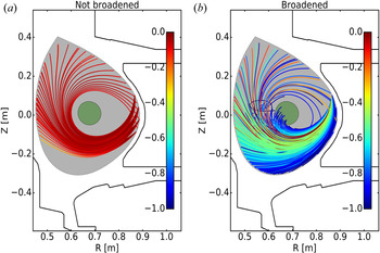
1. Introduction
Before an external radio-frequency (RF) wave can be dampened in the core plasma of a magnetic confinement device, it must first propagate through the highly turbulent scrape-off layer (SOL) region. SOL turbulence comprises dense, coherent structures called blobs/filaments (Zweben et al. Reference Zweben, Stotler, Terry, LaBombard, Greenwald, Muterspaugh, Pitcher, Group, Hallatschek and Maqueda2002; Kirk et al. Reference Kirk, Ayed, Counsell, Dudson, Eich, Herrmann, Koch, Martin, Meakins and Saarelma2006) that can significantly modify the incident wave spectrum. Scattering from filaments leads to refraction of the intended wave path and broadening of the incident wave spectrum, which in turn can cause lower efficiency in the intended function of the wave. For example, simulations predict significant power loss through filament-assisted mode conversion for launched ion cyclotron waves (Tierens, Zhang & Myra Reference Tierens, Zhang and Myra2020b). Electron cyclotron beams can be broadened in the presence of SOL turbulence, which leads to ineffective targeting of neo-classical tearing modes (Tsironis et al. Reference Tsironis, Peeters, Isliker, Strintzi, Chatziantonaki and Vlahos2009). In the case of driving current using lower hybrid (LH) waves, SOL scattering is a promising explanation for the spectral gap problem and current drive density limit.
Measurements on Alcator C-Mod (Mumgaard Reference Mumgaard2015), EAST (Ding et al. Reference Ding, Bonoli, Tuccillo, Goniche, Kirov, Li, Li, Cesario, Peysson and Ekedahl2018) and Tore Supra (Peysson et al. Reference Peysson2000) indicate self-similar, on-axis peaked LH current profiles. Ray tracing/Fokker–Planck simulations predict off-axis peaks (Mumgaard Reference Mumgaard2015), which are inconsistent with these measurements. In addition, these simulated profiles are sensitive to plasma and wave launch parameters, unlike experiment. Lastly, lower hybrid current drive (LHCD) suffers from an anomalous density limit, beyond which current drive (CD) efficiency dramatically falls (Wallace et al. Reference Wallace, Parker, Bonoli, Hubbard, Hughes, LaBombard, Meneghini, Schmidt, Shiraiwa and Whyte2010). Meanwhile, SOL turbulence increases with Greenwald density (Cziegler et al. Reference Cziegler, Terry, Hughes and LaBombard2010). Raising the Ohmic current, and therefore decreasing Greenwald density and shrinking the SOL width, is shown to increase the LHCD efficiency at high densities in C-Mod (Baek et al. Reference Baek, Wallace, Bonoli, Brunner, Faust, Hubbard, Hughes, LaBombard, Parker and Porkolab2018). These considerations suggest there are important spectral broadening effects, i.e. scattering from SOL turbulence, unaccounted for in the standard ray tracing/Fokker–Planck model.
It should be noted that alternate spectral broadening mechanisms exist. These include full-wave effects in the core like interference and focusing, and edge mechanisms such as parametric decay instabilities (PDIs) (Porkolab Reference Porkolab1977). The capability to run full-wave simulations of LHCD is fairly recent (Wright et al. Reference Wright, Bonoli, Schmidt, Phillips, Valeo, Harvey and Brambilla2009; Shiraiwa et al. Reference Shiraiwa, Meneghini, Parker, Bonoli, Garrett, Kaufman, Wright and Wukitch2010), and it is not yet clear whether it provides a better match to experiment than ray tracing/Fokker–Planck models. PDI is a strong candidate for explaining the current drive density limit (Cesario et al. Reference Cesario, Amicucci, Cardinali, Castaldo, Marinucci, Napoli, Paoletti, De Arcangelis, Ferrari and Galli2014; Baek et al. Reference Baek, Parker, Bonoli, Shiraiwa, Wallace, LaBombard, Faust, Porkolab and Whyte2015). However, there is no clear indication that PDI significantly modifies the wave spectrum in low-density discharges (Baek et al. Reference Baek, Parker, Bonoli, Shiraiwa, Wallace, LaBombard, Faust, Porkolab and Whyte2015). Note that the parallel wave vector up-shift from PDI and the perpendicular wave vector rotation from scattering may both be required to bridge the LH spectral gap (Biswas et al. Reference Biswas, Baek, Bonoli, Shiraiwa, Wallace and White2020). (The terms ‘perpendicular/parallel’ are used in relation to the local background magnetic field.)
Early attempts to model LH wave scattering in the SOL treat the turbulence as incoherent drift-wave-like density fluctuations (Bellan & Wong Reference Bellan and Wong1978; Bonoli & Ott Reference Bonoli and Ott1982; Andrews & Perkins Reference Andrews and Perkins1983). This results in a diffusive process leading to the angular broadening of the perpendicular wave vector component  $\boldsymbol {k}_{\perp }$. While these models can significantly broaden the incident wave spectrum, they have been unable to explain experimental measurements at either low or high densities (Peysson et al. Reference Peysson, Decker, Morini and Coda2011; Bertelli et al. Reference Bertelli, Wallace, Bonoli, Harvey, Smirnov, Baek, Parker, Phillips, Valeo and Wilson2013). A recent study models LH scattering from coherent SOL filaments with ray tracing (Biswas et al. Reference Biswas, Baek, Bonoli, Shiraiwa, Wallace and White2020). This results in an increased angle-broadening effect compared with previous models, which in turn leads to a relatively better match with experimental current drive measurement and reduced sensitivity to simulation parameters. Another recent study using full-wave simulations predict a large parasitic loss of LH power in the presence of SOL filaments (Lau et al. Reference Lau, Martin, Shiraiwa and Wallace2020). This is attributed to significant partial reflection and side scattering. In ray tracing, partial reflection is neglected and side scattering is likely underestimated.
These results motivate a closer study of wave scattering from filaments using a full-wave treatment. Unlike ray tracing, which only accounts for refraction and total reflection, a full-wave model also retains the physical optics effects of interference, diffraction and focusing. In addition, full-wave models can account for asymmetric scattering, which results in the rotation of  $\boldsymbol {k}_{\perp }$ in one preferential direction. Notably, this effect is ignored in ray tracing and other wave-kinetic models for LH wave scattering. This is discussed further in § 7.2.
In this paper, a hybrid method is introduced to efficiently calculate the full-wave effects of RF scattering through a slab layer composed of filaments. First, the scattered EM wave is calculated for an incident wave interacting with a single filament, which is modelled as an infinitely long cylinder. This problem has a semi-analytic solution, and can be very efficiently computed relative to numeric full-wave solvers. Previous implementations (Myra & D'Ippolito Reference Myra and D'Ippolito2010; Ram & Hizanidis Reference Ram and Hizanidis2016) of this semi-analytic scattering (SAS) model in a plasma-physics context were restricted to ‘flat-top’ (homogeneous) filaments. This model is generalized to filaments with radially varying density profiles, which better mimic experimentally relevant filaments. Next, a scattering width (analogous to a scattering cross-section) is calculated from the scattered wave solution. Third, this process is repeated multiple times, for different filament parameters, until a statistically averaged ‘effective’ scattering width is produced. Lastly, this effective scattering width is used to calculate the cumulative effect of multiple scattering events for an RF wave incident on a turbulent slab. This is identical to solving the radiative transfer equation, for which many techniques exist from the fields of optics and neutronics. The present study uses the absorbing Markov chain technique (Esposito & House Reference Esposito and House1978) to compute the final transmitted and reflected wave spectrum. This workflow is henceforth called the semi-analytic scattering Markov chain (SAS-MC) model.
The SAS-MC model can be applied to any frequency range to study RF scattering in the SOL because it is derived using the fully electromagnetic cold dispersion relation. This paper focuses on applying the model to LH waves. Assuming certain properties about the SOL geometry and turbulence, a modified wave spectrum is calculated for LH launching in a low-density Alcator C-Mod discharge. This wave spectrum is coupled to the ray tracing/Fokker–Planck solver GENRAY (Smirnov & Harvey Reference Smirnov and Harvey2001)/CQL3D (Harvey & McCoy Reference Harvey and McCoy1992) to determine its impact on current drive. The result is a significantly modified CD profile that is peaked on-axis. This increased on-axis damping is attributed to a fraction of LH rays rotated by scattering such that they dampen on-axis during the first pass. In addition, a mechanism for asymmetric scatter is identified. The extent of asymmetric scattering increases with background density and turbulence.
This paper is structured in the following way. Section 2 reviews the SAS model for calculating the scattered wave. In § 3, the SAS model is generalized to radially varying filaments. Section 4 discusses the calculation of the scattering width and ‘effective’ scattering width. Section 5 introduces the Markov chain (MC) model necessary to calculated the final modified wave spectrum following propagation through the SOL. In § 6, the SAS-MC model is compared with the higher-fidelity numeric full-wave solver PETRA-M (Shiraiwa et al. Reference Shiraiwa, Wright, Bonoli, Kolev and Stowell2017). Limitations on the accuracy of the SAS-MC model are discussed. Section 7 applies the SAS-MC model to lower hybrid launching in a typical SOL in C-Mod. There is an in-depth discussion about the asymmetric profile of the scattering width. Comparisons are made with a ray tracing treatment. In § 8, the modified wave spectrum is coupled to GENRAY/CQL3D to model LHCD in a C-Mod discharge. Section 9 summarizes the results of this study.
2. Review of semi-analytic scattering model
The first component of the SAS-MC model is the semi-analytic Mie-scattering description of an incident RF wave interacting with a single cylindrical filament. To the best of the authors’ knowledge, this problem was first treated in the magnetized plasma context by Myra & D'Ippolito (Reference Myra and D'Ippolito2010) in the lower hybrid limit ( $\varOmega _{ci}^{2} \ll \omega ^{2} \ll \varOmega _{ce}^{2}$) for a homogenous cylinder. Ram & Hizanidis (Reference Ram and Hizanidis2016) extended this model to all frequencies. The single filament scattering model is briefly reviewed in this section, and then extended to radially inhomogeneous filaments in § 3.
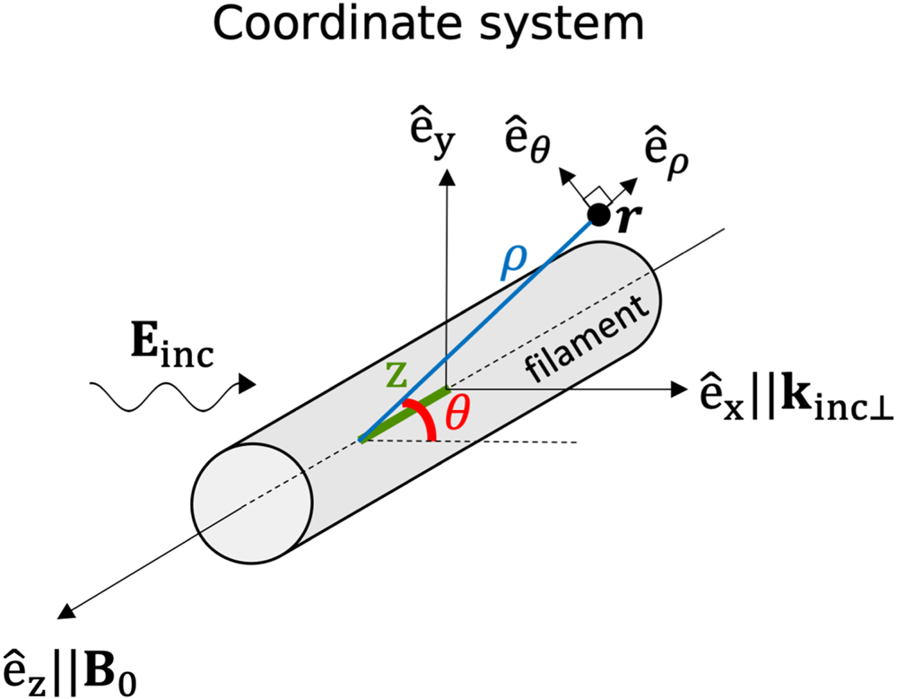
Figure 1 illustrates the SAS model coordinate system. The cylinder axis is aligned with the background magnetic field  $\boldsymbol {B}_0$ in the
 $z$-direction. Given a plane wave travelling in the
 $+x$-direction, the objective is to calculate the scattered wave exterior to the cylinder. The electric field inside and outside the filament must satisfy the vector wave equation. In the case that the cylinder's dielectric properties have no longitudinal (
 $z$) and poloidal (
 $\theta$) dependence, this problem can be solved via separation of variables in cylindrical coordinates.
Poloidal and Cartesian coordinate system used to model RF scattering from a field-aligned filament.

Because the medium is homogeneous inside and outside the cylinder, it is simple to formulate an ansatz to the wave equation in each region. There are five waves to consider: the known incident wave  $\boldsymbol {E}_{0}$; the scattered slow, fast wave
 $\boldsymbol {E}_{1}$,
 $\boldsymbol {E}_{2}$ outside the cylinder; and the slow, fast wave
 $\boldsymbol {E}_{3}$,
 $\boldsymbol {E}_{4}$ excited inside the cylinder. At the discontinuous boundary
 $\rho = a_b$, the fields inside and outside must satisfy Maxwell's boundary conditions.
2.1. Ansatz to electric field
Using separation of variables (see Appendix A), the electric field can be written in cylindrical coordinates as
 $$\begin{gather} E_{j \gamma} = \exp({\textrm{i}(k_{||}z-\omega t)})\sum_{m={-}\infty}^{+\infty} E_{jm} W_{j \gamma m} \exp({\textrm{i} m \theta}); \quad \gamma = \rho,\theta,z, \end{gather}$$
 $$\begin{gather}W_{j\rho m} = \xi_{jx} \textrm{J}_{m}^{\prime}(k_{j \perp}\rho) - \textrm{i}\xi_{jy} \frac{m}{k_{j \perp} \rho} \textrm{J}_{m}(k_{j \perp}\rho), \end{gather}$$
 $$\begin{gather}W_{j\theta m} = \textrm{i}\xi_{jx} \frac{m}{k_{j \perp} \rho} \textrm{J}_{m}(k_{j \perp}\rho) + \xi_{jy} \textrm{J}_{m}^{\prime}(k_{j \perp}\rho), \end{gather}$$
 $$\begin{gather}W_{jzm} = \textrm{i} \xi_{jz}\textrm{J}_{m}(k_{j \perp}\rho), \end{gather}$$
where  $j=0,\ldots,4$ is the wave index,
 $\boldsymbol{\xi}_j = \{\xi _{jx},\xi _{jy},\xi _{jz}\}$ is the plane-wave polarization of wave
 $j$,
 $\textrm {J}_{m}$ is the Bessel function of the first kind and order
 $m$, and
 $\textrm {J}_{m}^{\prime }$ is the first derivative of
 $\textrm {J}_{m}$ with respect to its argument. For the known incident plane wave (
 $\kern1.5pt j=0$), it is required that
 \begin{equation} E_{0m} = i^{m-1}, \end{equation}
as  $E_{jm}$ for
 $j>0$ have yet to be determined.
Note that  $k_{||}$ is the same for all waves, and is fixed by the incident wave. This is a consequence of Snell's law applied to a medium that is constant along the
 $z$-direction.
2.2. Boundary conditions
In general, the solutions in (2.1) can have both J and Y terms, where Y is the Bessel function of the second kind. The requirement that  $\boldsymbol {E}$ is finite at
 $\rho = 0$ leads to Y terms being zero for the slow and fast branch inside the filament. For
 $\rho \rightarrow \infty$, the scattered fields must be radiating away from the filament. For the scattered fast wave, this requires the use of Hankel functions of the first kind,
 $H^{1}$, instead of J in (2.1). The LH slow wave is backward propagating, which means
 $\boldsymbol {k}_{\perp }$ and
 $\boldsymbol {v}_{gr,\perp }$ are anti-parallel. This requires the use of Hankel functions of the second kind,
 $H^{2}$, for the scattered slow wave.
It should be noted that a backward-propagating incident wave (i.e. the slow wave) has  $k_{\textrm {inc},x} = -k_{\perp }$. This flipped sign can most easily be accounted for by substituting
 $\textrm {J}_{m} \rightarrow \textrm {J}_{-m}$ (Myra & D'Ippolito Reference Myra and D'Ippolito2010).
Lastly, a system of equations must be formulated to determine coefficients  $E_{jm}$ for
 $j=1,\ldots,4$. This is accomplished by imposing the four independent Maxwell boundary conditions at
 $\rho = a_b$ (see Appendix B). For each poloidal mode number, there are four unknown coefficients and four boundary conditions, which results in a solvable system of equations.
3. Generalizing to radially inhomogeneous filaments
The scattering model reviewed in the previous section is now extended to account for radially inhomogeneous cylinders. The cylinder remains poloidally symmetric, and therefore the poloidal mode numbers are still uncoupled. A solution via separation of variables, similar to that in § 2, is still possible. The following solution scheme for a radially inhomogeneous filament is similar to Mie-scattering techniques for layered dielectrics (Kai & d'Alessio Reference Kai and d'Alessio1995) or annular cylinders (Wu Reference Wu1994). Recently, a similar scheme has been used to model scattering and mode conversion of the ion cyclotron wave in the presence of Gaussian filaments (Zhang et al. Reference Zhang, Tierens, Bobkov, Cathey, Cziegler, Griener, Hoelzl and Kardaun2021).
In the previous case of a totally homogeneous ‘flat-top’ cylinder, there was a single boundary (at  $\rho = a_b$) and therefore only one radial ‘bin’ inside the cylinder. The cylinder is now discretized into multiple bins
 $r=0,\ldots,R$. In other words, the filament is now a set of radially stratified concentric cylinders. This introduces discontinuities in the media between bins, and so boundary conditions must be imposed at each separating layer. In the limit
 $R \rightarrow \infty$, a cylinder with a smoothly varying radial profile can be modelled with arbitrary precision.
3.1. Modified system of equations
Remember that the ‘flat-top’ ( $R=0$) system is solvable because there exist four unknowns
 $E_1,E_2,E_3,E_4$ and four independent boundary equations for each mode number
 $m$. A similar system of equations must be derived for the general
 $R>0$ case. The simplest case (
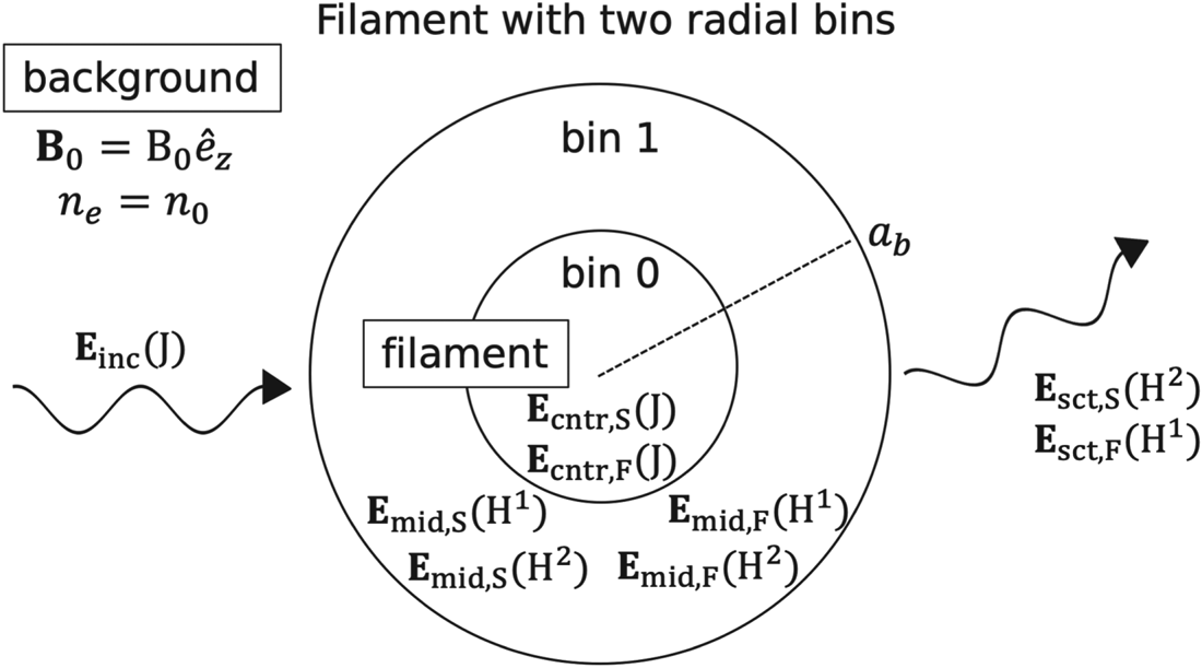
 $R=1$) is illustrated in figure 2. In the intermediate layers (
 $0< r \leq R$), each wave branch is generally a function of both
 $H_{m}^{1}$ and
 $H_{m}^{2}$ terms, and are therefore split into these two electric field contributions.
The different contributions of  $\boldsymbol {E}$ in the SAS model for a filament with two radial bins (
 $R=1$). There are two regions of interest: background and filament. The filament is further divided into the central (cntr) and intermediate (mid) regions. Here ‘
 $S$’ and ‘
 $F$’ denote slow and fast LH branches. Functions in parentheses denote the type of Bessel function used in (2.1).

With the considerations made above, there are now eight unknown waves for the  $R=1$ case. There are also two boundaries, which supply four boundary conditions each. This results in a solvable system for the total electric field everywhere.
For the general case ( $R>0$), there are all together
 $4(R+1)$ equations for each mode number. For more details, see Appendix C. Solving for the total electric field requires inverting
 $4(R+1) \times 4(R+1)$ matrices a total of
 $2M+1$ times, where
 $M$ is the maximum mode number chosen to truncate the series. These matrices are sparse and banded, which results in fast solution times of the order of seconds on a single central processing unit (CPU).
3.2. Poloidal and radial resolution
The electric field will evolve on three possible length scales:  $a_b, k_{\text {in} \perp }^{-1}$ or
 $k_{\text {out} \perp }^{-1}$. Subscripts ‘in’, ‘out’ denote inside, outside the cylinder. Define a characteristic poloidal mode number
 $\tilde {m} \equiv \text {max}(k_{\text {in} \perp },k_{\text {out} \perp })a_{b}$. If
 $\tilde {m} \gtrsim 1$, terms with
 $|m|>\tilde {m}$ will rapidly decay in magnitude. Therefore, for a converged solution, it is necessary that
 $M \gg \tilde {m}$. If
 $\tilde {m}\ll 1$, it is necessary that
 $M \gg 1$.
A rule-of-thumb can also be derived for how many radial bins are required. The source of error stems from discretizing the cylinder's smoothly varying radial profile into homogeneous radial bins. The discontinuity between bins is of the order of  $L_{n}^{-1} \Delta r$, where
 $L_n$ is the characteristic length of the density inhomogeneity. Here,
 $\Delta r$ is the radial bin width. Assume the cylinder has a monotonically decreasing radial profile with characteristic radial width
 $a_b$. Then the discontinuity is approximately
 $L_{n}^{-1} \Delta r \sim ( {n_b}/{n_0 a_b}) ( {a_b}/{R}) = {n_b}/{n_0 R}$. Here
 ${n_b}/{n_0}$ is the ratio of the peak (centre) cylinder density to the background density, and
 $R$ is the number of radial bins. To ensure the discontinuities are small requires
 $R \gg {n_b}/{n_0}$.
4. Scattering width for statistical ensemble of filaments
While the model described above solves for the scattered field, it is more convenient to calculate a differential scattering width, which accounts for the deflection of scattered power in  $\theta$-space. The differential scattering width is defined as (Myra & D'Ippolito Reference Myra and D'Ippolito2010)
 \begin{equation} \sigma(\theta) \equiv \frac{\textrm{d}\sigma}{\textrm{d}\theta} = \frac{\textrm{lim}_{\rho \rightarrow \infty} \rho S_{\textrm{sct},\rho}(\rho,\theta)}{S_{\textrm{inc},x}},\end{equation}
where  $\boldsymbol {S}_{\textrm {inc}}$,
 $\boldsymbol {S}_{\textrm {sct}}$ is the incident, scattered Poynting flux. It follows that the scattering width
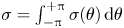 $\sigma = \int _{-{\rm \pi} }^{+{\rm \pi} } \sigma (\theta ) \,\textrm {d}\theta$. See Appendix D for the derivation and physical meaning of
 $\sigma$. The scattering width (units of length) is the one-dimensional (1-D) analogy for a scattering cross-section (units of length squared).
Lastly, define a normalized differential scattering width  $\hat {\sigma }(\theta ) = \sigma (\theta )/\sigma$, which will be useful in § 5. Note that
 $\sigma (\theta ) \geq 0$ because at a far enough distance, the scattered waves must be radiating away from the cylinder.
So far, no explicit expressions for  $S_{\textrm {sct},\rho }$ and
 $S_{\textrm {inc},x}$ in (4.1) have been provided. The time-averaged Poynting flux for the scattered wave can be written as
 \begin{equation} \boldsymbol{S}_{sct,j}= \frac{1}{2 \mu_0 \omega} \textrm{Im}\,{\boldsymbol{E}_{j}^{*} \times (\boldsymbol{\nabla} \times \boldsymbol{E}_{j})}, \end{equation}
where  $j = S,F$ now refer to the scattered slow and fast wave, respectively. Equation (2.1) is substituted into (4.2) and then substituted into (4.1) to produce
 \begin{equation} \sigma_{j}(\theta) = \frac{ \mp 2}{\rm \pi} \frac{|\xi_{j,y}|^{2} + |\xi_{j,z}|^{2} + \dfrac{k_z}{k_{j\perp}} \textrm{Re}\,{\xi_{j,x} \xi_{j,z}^{*}} }{k_{\textrm{inc},x} (|\xi_{\textrm{inc},y}|^{2} + |\xi_{\textrm{inc},z}|^{2}) -k_{z} \textrm{Re}\,{\xi_{\textrm{inc},x} \xi_{\textrm{inc},z}^{*}}} \left|{\sum_{m={-}\infty}^{+\infty}i^{{\pm} m} E_{jm} \textrm{e}^{\textrm{i} m \theta}}\right|^{2},\end{equation}
assuming real valued  $k_{j\perp }$. If
 $k_{j\perp }$ is imaginary, then the right-hand side of (4.3) is zero. Here,
 $\sigma _{(S,F)} (\theta )$ denotes the differential scattering width for coupling from the incident slow wave to a scattered slow, fast wave. The asymptotic relation
 $H_{m}^{(1,2)}(\tau )\approx \sqrt {({2}/{{\rm \pi} \tau }})\exp ({\pm \textrm {i}(\tau -m {\rm \pi}/2 - {\rm \pi}/4)})$ for large argument
 $\tau$ has been used. In the denominator,
 $\boldsymbol {\xi }_{\textrm {inc}}$ is the normalized polarization of the incident slow wave. Equation (4.3) is a generalization of the
 $\sigma (\theta )$ calculated by Myra & D'Ippolito (Reference Myra and D'Ippolito2010), which was done in the electrostatic limit. Equation (4.3) accounts for a fully electromagnetic dispersion tensor, and is therefore valid for the low densities in the far-SOL.
The total differential scattering width is
 \begin{equation} \sigma(\theta) = \sigma_{S}(\theta) + \sigma_{F}(\theta). \end{equation}
For background densities in which the slow wave is propagating but the fast wave is evanescent,  $\sigma _{F} = 0$. It only becomes comparable to
 $\sigma _S$ as the background density approaches the mode-conversion density. For the purposes of studying slow-wave scattering in the SOL, it is reasonable to neglect
 $\sigma _{F}$.
4.1. Effective differential scattering width:  $\sigma _{\text {eff}}(\theta )$

In the presence of a filament, the resulting scattered field will depend on  $a_b$ and
 $n_{b}$. Therefore,
 $\sigma (\theta )= \sigma (\theta ; n_b/n_0, a_b)$ for a given
 $n_0, \boldsymbol {B},N_{||}$ and
 $\omega$. A joint probability distribution function (p.d.f.),
 $p(n_b/n_0,a_b)$, is introduced. This is the probability that a filament will have certain parameters
 $a_b$ and
 $n_b/n_0$. Taking a weighted average of
 $\sigma (\theta )$ with this joint-p.d.f. returns the statistically averaged
 $\sigma (\theta )$ for scattering from a randomly selected filament. This averaged, or ‘effective’ differential scattering width is defined as
 \begin{equation} \sigma_{\text{eff}}(\theta) = \int_{0}^{\infty} \textrm{d}a_{b} \int_{0}^{\infty}\textrm{d} \left(n_{b}/n_0\right) \sigma_{S}(\theta; n_b/n_0, a_b) p(n_b/n_0,a_b), \end{equation}
where  $p(n_b/n_0,a_b)$ is normalized such that
 $\int _{0}^{\infty } \textrm {d}a_{b} \int _{0}^{\infty }\textrm {d}(n_{b}/n_0)p(n_b/n_0,a_b) = 1$. Again,
 $\sigma _{F}$ is neglected because the focus is on SOL plasmas.
The choice of joint-p.d.f. for the filament parameters is guided by experimental measurements. In the SOL of C-Mod, mirror Langmuir probe measurements reveal positively skewed p.d.f.s of density fluctuations (Graves et al. Reference Graves, Horacek, Pitts and Hopcraft2005). SOL fluid codes predict that the filament width and density are positively correlated (Decristoforo et al. Reference Decristoforo, Militello, Nicholas, Omotani, Marsden, Walkden and Garcia2020). Therefore, the joint-p.d.f. is reasonably well described by a positively skewed normal p.d.f. for each parameter ( $n_b/n_0$ and
 $a_b$) along with a positive bivariate correlation. The analytic form for this p.d.f., as a function of a two-dimensional (2-D) column vector
 $\boldsymbol{\zeta} = [ n_b/n_0; a_b ]$ is (Azzalini & Capitanio Reference Azzalini and Capitanio1999)
 $$\begin{gather} p(\boldsymbol{\zeta}) = 2 \phi_{2}(\boldsymbol{\zeta} - \boldsymbol{Q},\boldsymbol{\varOmega}) \varPhi(\boldsymbol{\varGamma}^{\text{T}} \boldsymbol{\cdot} (\boldsymbol{\zeta}-\boldsymbol{Q})), \end{gather}$$
 $$\begin{gather}\boldsymbol{\varOmega} = \begin{bmatrix} s_{n_b/n_0}^{2} & \eta s_{n_b/n_0} s_{a_b}\\ \eta s_{n_b/n_0} s_{a_b} & s_{a_b}^{2} \end{bmatrix}, \end{gather}$$
 $$\begin{gather}\boldsymbol{Q} = \langle \boldsymbol{\zeta} \rangle - \sqrt{\frac{2}{\rm \pi}} \boldsymbol{\delta} \end{gather}$$
 $$\begin{gather}\boldsymbol{\delta} = \frac{1}{\sqrt{1 + \boldsymbol{\varGamma}^{\text{T}}\boldsymbol{\cdot} \boldsymbol{\varOmega}\boldsymbol{\cdot} \boldsymbol{\varGamma}}} \boldsymbol{\varOmega} \boldsymbol{\cdot} \boldsymbol{\varGamma}, \end{gather}$$
 $$\begin{gather}\boldsymbol{\varGamma} = \begin{bmatrix} \varGamma_{n_b/n_0}\\ \varGamma_{a_b} \end{bmatrix}, \end{gather}$$
where  $\phi _{2}(\boldsymbol{\zeta},\boldsymbol{\varOmega})$ is a 2-D normal p.d.f. with zero mean and correlation matrix
 $\boldsymbol{\varOmega}$. Here
 $\varPhi (x)$ is the 1-D normal cumulative distribution function (CDF) for scalar input
 $x$,
 $\boldsymbol{\varGamma}$ is a 2-D column vector of skewness factors and
 $\langle \boldsymbol{\zeta} \rangle \equiv [ \langle n_b/n_0 \rangle ; \langle a_b\rangle ]$ is the 2-D column vector of mean
 $n_b/n_0$ and
 $a_b$. Similarly,
 $\boldsymbol{s} \equiv [s_{n_b/n_0}; s_{a_b}]$ are standard deviations and
 $\eta$ is the scalar correlation coefficient. It is therefore possible to parametrize
 $p(\boldsymbol{\zeta})$ as a function of
 $\langle \boldsymbol{\zeta} \rangle, \boldsymbol{\varGamma}, \boldsymbol{s}$ and
 $\eta$.
Filament mean width  $\langle a_b \rangle$ is well bounded by gas puff imaging (GPI) measurements as well as theory/simulation (Zweben et al. Reference Zweben, Stotler, Terry, LaBombard, Greenwald, Muterspaugh, Pitcher, Group, Hallatschek and Maqueda2002; Krasheninnikov, D'Ippolito & Myra Reference Krasheninnikov, D'Ippolito and Myra2008; Keramidas Charidakos et al. Reference Keramidas Charidakos, Myra, Ku, Churchill, Hager, Chang and Parker2020). Langmuir probe and GPI measurements provide a rough lower bound on the filament mean relative density
 $\langle n_b/n_0 \rangle$, though this value will vary significantly at different radial locations in the SOL (Zweben et al. Reference Zweben, Stotler, Terry, LaBombard, Greenwald, Muterspaugh, Pitcher, Group, Hallatschek and Maqueda2002; Terry et al. Reference Terry, Zweben, Hallatschek, LaBombard, Maqueda, Bai, Boswell, Greenwald, Kopon and Nevins2003).
5. The radiative transfer equation in slab geometry
The previous sections deal with a single scattering event arising from one filament. Section 4.1 introduced an effective scattering width  $\sigma _{\text {eff}}(\theta )$, but this still only gives information about the average scattered power arising from one filament. Consider a turbulent medium with filaments of mean width
 $\langle a_b \rangle$ with packing fraction
 $f_{p}$. An incident LH wave will, on average, interact with
 ${f_p L_x}/{{\rm \pi} \langle a_{b} \rangle ^{2}}$ filaments per unit length in the perpendicular plane. Therefore,
 $\varSigma _{\text {eff}} \equiv (\,{f_p}/{{\rm \pi} \langle a_b \rangle ^{2}})\sigma _{\text {eff}}$ is the inverse mean-free-path for the incident power to scatter. A radiative transfer equation (RTE) can then be derived as
 \begin{align} \left(\frac{\partial}{\partial t} + \boldsymbol{v}_{gr} \boldsymbol{\cdot} \boldsymbol{\nabla} \right) P(\boldsymbol{r},\theta)={-}\varSigma_{\text{eff}} |\boldsymbol{v}_{gr \perp}| P(\boldsymbol{r},\theta) + \varSigma_{\text{eff}} |\boldsymbol{v}_{gr \perp}| \int_{-{\rm \pi}}^{\rm \pi}\hat{\sigma}_{\text{eff}}(\theta-\theta^{\prime})P(\boldsymbol{r},\theta^{\prime})\, \textrm{d}\theta^{\prime}, \end{align}
where  $P(\boldsymbol {r},\theta )$ is the power density at
 $\boldsymbol {r}$ directed along angle
 $\theta$. In (5.1), the first term on the right-hand side accounts for the power directed along
 $\theta$ that is lost to scattering. The second term accounts for the power gained at
 $\theta$ owing to scattering from all other
 $\theta ^{\prime }$. (Any losses arising from the anti-Hermitian part of the dielectric tensor are ignored.)
Now, consider a steady-state slab geometry with a filamentary turbulent layer limited to  $0< x< L_{x}$. The filaments and background
 $B$ are aligned along the
 $z$-direction. An LH plane wave is incident on the slab from the left (
 $S_{\textrm {inc},x}>0$). Because the background density is homogeneous,
 $|\boldsymbol {v}_{gr\perp }|$ is constant. Equation (5.1) then simplifies to
 $$\begin{gather} \cos\theta \frac{\textrm{d}P(x,\theta)}{\textrm{d} x} ={-} \varSigma_{\text{eff}}P(x,\theta) + \varSigma_{\text{eff}}\int_{-{\rm \pi}}^{\rm \pi}\hat{\sigma}_{\text{eff}} (\theta-\theta^{\prime})P(x,\theta^{\prime})\,\textrm{d}\theta^{\prime}, \end{gather}$$
 $$\begin{gather}P(L_{x},\theta) = 0 \quad \textrm{for} \ |\theta| \geq {\rm \pi}/2, \end{gather}$$
 $$\begin{gather}P(0,\theta) = \delta(\theta) \quad \textrm{for} \ |\theta| \leq {\rm \pi}/2, \end{gather}$$
where  $\delta (\theta )$ is the Dirac delta function. Compare this to (31) in Andrews & Perkins (Reference Andrews and Perkins1983), where a similar RTE was formulated for drift-wave-like turbulence. Equations (5.2b) and (5.2c) enforce no scattering back into the turbulent layer at
 $x = L_{x}$ and
 $0$, respectively. Equation (5.2c) also enforces a normalized incident power from the left. Solving this equation and evaluating
 $P(x,\theta )$ at
 $x = L_x$ and
 $0$ results in the normalized angle-broadened transmitted and reflected wave spectra, respectively.
It should be noted that two critical assumptions have been made in formulating the RTE: (1)  $\sigma _{\text {eff}} (\theta )$ is formulated using the far-field limit; (2) the interaction of a wave with multiple filaments is modelled by chaining multiple single-filament scattering events. Together, they constitute the far-field approximation, which is only valid if
 $\langle a_b \rangle \ll d$ and
 $k_{\perp } d \gg 1$, where
 $d$ is the average distance between filaments (Mishchenko Reference Mishchenko2014). This approximation breaks down as
 $f_p$ increases (and therefore
 $d$ decreases) and is further discussed in § 6.2.
5.1. Solution to RTE using a Markov chain
Equation (5.2) is an integro-differential equation, and cannot, in general, be solved analytically. One numerical method is to discretize the wave spectrum into photons/rays, and stochastically evolve their trajectories, as per the standard Monte Carlo technique. This method is rather slow in providing a converged wave spectrum near  $\theta = \pm {\rm \pi}/2$, where tally counts are usually low. Given how simple the slab geometry is, a more elegant absorbing Markov chain method can be employed. This Markov chain (MC) method is deterministic, so it avoids the low tally count problem. It is commonly used to solve for a reflected and transmitted wave spectrum through a turbid slab (e.g. solar rays interacting with Earth's atmosphere). The present study closely follows the formalism by (Esposito & House Reference Esposito and House1978) and Xu et al. (Reference Xu, Davis, West and Esposito2011).
Power is incident on the turbulent slab from the left, directed along the  $x$-direction (
 $\theta _{0}=0$). It is convenient to define a
 $\zeta \equiv |\cos {\theta }|$ such that
 $\zeta _{0}=1$. It is simple to calculate the fraction of transmitted power that does not scatter in the slab. This is the ‘ballistic’ fraction:
 \begin{equation} P_{\textrm{ball}} = \exp\left({-\frac{L_x}{\zeta_{0}}\varSigma_{\text{eff}}}\right).\end{equation}
It is also straightforward to calculate the transmitted and reflected fraction that only scatter once in the slab:
 \begin{align} P_{T,1}(\theta) &= \hat{\sigma}(\theta-\theta_{0}) \exp\left({-\frac{L_{x}}{\zeta}\varSigma_{\text{eff}}}\right)\nonumber\\ &\quad \times \begin{cases} 0 & \cos{\theta} < 0,\\ \dfrac{\zeta \zeta_{0}}{\zeta-\zeta_{0}}\left[1- \exp\left({-L_{x}\varSigma_{\text{eff}}\left(\dfrac{1}{\zeta_0}-\dfrac{1}{\zeta}\right)}\right)\right] & \theta \neq \theta_{0},\\ \varSigma_{\text{eff}}L_{x} & \theta = \theta_0, \end{cases} \end{align}
 \begin{equation} P_{R,1}(\theta) = \hat{\sigma}(\theta-\theta_{0}) \times \begin{cases} 0 & \cos{\theta} > 0,\\ \dfrac{\zeta \zeta_{0}}{\zeta+\zeta_{0}}\left[1-\exp\left({-}L_{x}\varSigma_{\text{eff}}\left(\dfrac{1}{\zeta_0}+\dfrac{1}{\zeta}\right)\right)\right] & \text{otherwise}. \end{cases}\end{equation}
The above are the first-order scattering terms. To compute the higher-order terms (fraction of power undergoing  $> 1$ scattering events), it is necessary to use the MC method. The slab is discretized into
 $n=1,\ldots,{N}$ segments of width
 $\Delta x=L_{x}/{N}$. The angular spectrum is also discretized into
 $m=1,\ldots,{M}$ segments of width
 $\Delta \theta =2{\rm \pi} /{M}$. Next, the
 $\text {NM}\times \text {NM}$ ‘transition’ matrix
 $\boldsymbol{T}(x_n,\theta _m;x_{n^{\prime }}\theta _{m^{\prime }})$ is generated, which accounts for the probability of a photon in segment
 $n$ and directed along
 $\theta _m$ to scatter in segment
 $n'$ into
 $\theta _{m^{\prime }}$. The
 ${N}\times {M}$ ‘source’ matrix
 $\boldsymbol{\varPi} (x_n,\theta _m)$ is defined as the probability distribution of photons in segment
 $n$ directed along
 $\theta _{m}$ right after the first scattering event. Lastly, the
 $\text {NM}\times {M}$ ‘absorption’ matrix
 $\boldsymbol{R}_{T/R}(x_n,\theta _m;\theta _{m^{\prime }})$ is the probability of a photon to escape the slab via transmission/reflection following its final scattering event in segment
 $n$ from
 $\theta _m$ to
 $\theta _{m^{\prime }}$. The form for these matrices are as follows. The ‘transition’ matrix can be broken into four components:
 \begin{equation} \boldsymbol{T}(x_n,\theta_m;x_{n^{\prime}}\theta_{m^{\prime}}) = p_{\text{esc}}(x_n,\theta_m)\,p_{\text{trvl}}(x_n, \theta_m, x_{n'})\, p_{\text{sct}}(x_{n'},\theta_m)\,\hat{\sigma}(\theta_{m'}-\theta_{m}), \end{equation}
where
 $$\begin{gather} p_{\text{esc}}(x_n,\theta_m) = \frac{\zeta_m}{\varSigma_{\text{eff}}\Delta x} \left(1-\exp\left({-\frac{\Delta x}{\zeta_m}\varSigma_{\text{eff}}}\right)\right), \end{gather}$$
 $$\begin{gather}p_{\text{trvl}}(x_n,\theta_m,x_{n'}) = \begin{cases} \exp\left({-\dfrac{x_{n'}-x_n}{\zeta_m}\varSigma_{\text{eff}}}\right) & \dfrac{x_{n'}-x_n}{\cos{\theta_m}} \geq 0,\\ 0 & \dfrac{x_{n'}-x_n}{\cos{\theta_m}} < 0,\end{cases} \end{gather}$$
 $$\begin{gather}p_{\text{sct}}(x_{n'},\theta_m) = 1 - \exp\left({-\frac{\Delta x}{\zeta_m}\varSigma_{\text{eff}}}\right). \end{gather}$$
The escape probability,  $p_{\text {esc}}(x_n,\theta _m)$, is the probability for a photon to travel through segment
 $n$ without scattering. The travel probability,
 $p_{\text {trvl}}(x_n,\theta _m,x_{n'})$, is the probability of travelling between segments
 $n$ and
 $n'$ without scattering. Note that
 $p_{\text {trvl}}$ is set to zero in cases where the photon in segment
 $n$ with
 $\theta _m$ is oriented such that it is travelling away from
 $n'$. The scatter probability,
 $p_{\text {sct}}(x_{n'},\theta _m)$, is the probability of scattering within segment
 $n'$. Lastly,
 $\hat {\sigma }(\theta _{m'}-\theta _{m})$ is the probability of the photon rotating from
 $\theta _m$ to
 $\theta _{m'}$ given that it undergoes a scattering event. The ‘source’ matrix is
 \begin{gather} \hspace{-18pc} \boldsymbol{\varPi} (x_n,\theta_m) = \hat{\sigma}(\theta_m-\theta_{0})C^{{-}1}\nonumber\\ \hspace{2.5pc}\times \begin{cases} \dfrac{\zeta_m}{\zeta_m-\zeta_0} \exp\left({-\left(\dfrac{x_n}{\zeta_0}+\dfrac{\Delta x}{\zeta_m}\right)\varSigma_{\text{eff}}}\right) & {}\\ \quad\times\left(1-\exp\left({-\varSigma_{\text{eff}}\Delta x \left(\dfrac{1}{\zeta_{0}}- \dfrac{1}{\zeta_m}\right)}\right)\right) & \cos{\theta_m} > 0,\\ \dfrac{\zeta_0 \zeta_m}{\zeta_0 + \zeta_m} \exp\left({-\dfrac{x_n}{\zeta_0}\varSigma_{\text{eff}}}\right) & {}\\ \quad\times\left(1 - \exp\left({-\varSigma_{\text{eff}}\Delta x \left(\dfrac{1}{\zeta_0}+\dfrac{1}{\zeta_m}\right)} \right)\right) & \cos{\theta_m} < 0,\\ \dfrac{\varSigma_{\text{eff}} \Delta x }{\zeta_0} \exp\left({-\dfrac{x_n + \Delta x}{\zeta_0}\varSigma_{\text{eff}}}\right) & \theta_m = \theta_0, \end{cases} \end{gather}
 \begin{gather} C = \frac{\zeta_m}{\varSigma_{\text{eff}}\Delta x} \left(1-\exp\left({-\frac{\Delta x}{\zeta_m}\varSigma_{\text{eff}}}\right)\right),\end{gather}
where the coefficient  $C$ is required to properly volume-average the source over segment
 $n$. The transmission and reflection ‘absorption’ matrices are
 \begin{align} \boldsymbol{R}_{T}(x_n,\theta_m;\theta_{m'}) &= \hat{\sigma}(\theta_{m'}-\theta_{m}) \nonumber\\ &\quad \times \begin{cases} 0 & \cos{\theta_{m'}} < 0,\\ \dfrac{\zeta_{m'}}{\zeta_{m'}-\zeta_m} \exp\left({-\varSigma_{\text{eff}}\left(\dfrac{L_x}{\zeta_{m'}} - \dfrac{x_n}{\zeta_{m}}\right)}\right) & {}\\ \quad\times\left(\exp\left({-\varSigma_{\text{eff}}x_n \left(\dfrac{1}{\zeta_{m'}} - \dfrac{1}{\zeta_{m}}\right)}\right) \right. & {}\\ \quad \left.- \exp\left({-\varSigma_{\text{eff}}L_x \left(\dfrac{L_x}{\zeta_{m'}} - \dfrac{x_n}{\zeta_{m}}\right)}\right)\right) & \cos{\theta_{m}} > 0,\\ \dfrac{\zeta_{m'}}{\zeta_m+\zeta_{m'}}\exp\left({-\varSigma_{\text{eff}} \left(\dfrac{L_x}{\zeta_{m'}}+\dfrac{x_n}{\zeta_m}\right)}\right) & {}\\ \quad \times\left(\exp\left({\varSigma_{\text{eff}}x_n\left(\dfrac{1}{\zeta_m}+ \dfrac{1}{\zeta_{m'}}\right)}\right)\right. & {}\\ \quad - \left.\exp\left({\varSigma_{\text{eff}}L_x\left(\dfrac{1}{\zeta_m}-\dfrac{1}{\zeta_{m'}}\right)}\right)\right) & \cos{\theta_{m}} < 0,\\ \dfrac{\varSigma_{\text{eff}}}{\zeta_m} \exp\left({-\varSigma_{\text{eff}}\left(\dfrac{L_x}{\zeta_{m'}}-\dfrac{x_n}{\zeta_m}\right)}\right) (L_x - x_n) & \theta_m = \theta_{m'}, \end{cases} \end{align}
 \begin{align} \boldsymbol{R}_{R}(x_n,\theta_m;\theta_{m'}) &= \hat{\sigma}(\theta_{m'}-\theta_{m}) \nonumber\\ &\quad \times \begin{cases} 0 & \cos{\theta_{m'}} > 0,\\ \dfrac{\zeta_{m'}}{\zeta_{m}-\zeta_{m'}} \exp\left({-\varSigma_{\text{eff}}\dfrac{x_n}{\zeta_{m}}}\right) & {}\\ \quad \times\left(1 - \exp\left({-\varSigma_{\text{eff}}x_n \left(\dfrac{1}{\zeta_{m'}} - \dfrac{1}{\zeta_{m}}\right)}\right)\right) & \cos{\theta_{m}} < 0,\\ \dfrac{\zeta_{m'}}{\zeta_m+\zeta_{m'}} \exp\left({\varSigma_{\text{eff}}\dfrac{x_n}{\zeta_{m'}}}\right) & {}\\ \quad \times \left(\exp\left({-\varSigma_{\text{eff}}x_n\left(\dfrac{1}{\zeta_m}+\dfrac{1}{\zeta_{m'}}\right)}\right) - 1\right) & \cos{\theta_{m}} > 0,\\ \dfrac{\varSigma_{\text{eff}}}{\zeta_m} \exp\left({-\dfrac{\varSigma_{\text{eff}}}{\zeta_{m'}}x_n}\right)x_n & \theta_m = \theta_{m'}. \end{cases} \end{align}
Using these matrices, one can calculate the higher-order transmitted/reflected wave spectrum terms:
 $$\begin{gather} \boldsymbol{P}_{T/R,2}(\theta_m) = \boldsymbol{\varPi} \boldsymbol{\cdot} \boldsymbol{I} \boldsymbol{\cdot} \boldsymbol{R}_{T/R}, \end{gather}$$
 $$\begin{gather} \boldsymbol{P}_{T/R,l}(\theta_m) = \boldsymbol{\varPi} \boldsymbol{\cdot} \boldsymbol{T}^{l-2} \boldsymbol{\cdot} \boldsymbol{R}_{T/R} \quad \text{for } l \geq 3, \end{gather}$$
where  $l$ is the order of the scattering term and
 $\boldsymbol{I}$ is the
 $\text {NM}\times \text {NM}$ identity matrix. In summing all scattering terms, the total transmitted and reflected wave spectrum is
 $$\begin{gather} \boldsymbol{P}_{T}(\theta_m) - \frac{P_{\textrm{ball}}}{\Delta \theta}\delta_{\theta_m,\theta_0} = \boldsymbol{P}_{T,1}(\theta_m) + \sum_{l=1}^{\infty} \boldsymbol{P}_{T,l}, \end{gather}$$
 $$\begin{gather} \boldsymbol{P}_{R}(\theta_m) = \boldsymbol{P}_{R,1}(\theta_m) +\sum_{l=1}^{\infty} \boldsymbol{P}_{R,l}, \end{gather}$$
and  $\delta _{i,j}$ is the Kronecker delta. Furthermore, (5.13a) can be rewritten as
 \begin{equation} \boldsymbol{P}_{T}(\theta_m) - \frac{P_{\textrm{ball}}}{\Delta \theta}\delta_{\theta_m,\theta_0} - \boldsymbol{P}_{T,1}(\theta_m)= \boldsymbol{\varPi} \boldsymbol{\cdot} \left( \boldsymbol{I} + \sum_{l=1}^{\infty} \boldsymbol{T}^{l} \right) \boldsymbol{\cdot} \boldsymbol{R}_{T} = \boldsymbol{\varPi} \boldsymbol{\cdot} \left( \boldsymbol{I} - \boldsymbol{T}\right)^{{-}1}\boldsymbol{\cdot} \boldsymbol{R}_{T}.\end{equation}
A similar form applies to (5.13b). The second relation in (5.14) produces the solution following a matrix inversion. In practice, it is often faster to evaluate the first relation and truncate the series at a finite  $l$ when the solution is sufficiently converged (Yang et al. Reference Yang, Xiao, Li and Ma2018).
In deriving  $p_{\text {esc}}$ and
 $p_{\text {sct}}$, the possibility of multiple scattering events in segment
 $n$ is neglected. This is a reasonable assumption as long as
 $\Delta x \equiv {L_x}/{{N}} \ll {\zeta }/{\varSigma _{\text {eff}}}$. The population of photons with
 $\zeta \approx 0$ is the largest source of error for any finite
 $N$. Nevertheless, in practice,
 $\boldsymbol{P}_{T/R}$ is found to converge as long as
 $\varSigma _{\text {eff}} \Delta x \ll 1$. A criterion for the angular resolution is not as straightforward. It depends on the smoothness of
 $\hat {\sigma }(\theta )$. Naturally, a fine resolution is needed to accurately resolve sharp peaks in
 $\hat {\sigma }(\theta )$.
6. Verification of SAS-MC with numeric full-wave solver
The SAS-MC model is compared with the higher-fidelity finite-element full-wave code PETRA-M (Shiraiwa et al. Reference Shiraiwa, Wright, Bonoli, Kolev and Stowell2017). First, the SAS model for a single filament is compared with PETRA-M. Then the same is done for the MC model, which accounts for multiple filaments in a slab.
6.1. Scattered field for single filament
Consider an incident slow wave with a prescribed frequency  $f$ and parallel refractive index
 $N_{||}\equiv {c k_{||}}/{\omega }$. Also assume a filament with Gaussian radial profile such that
 \begin{equation} n(\rho) -n_0= n_0 \left( \frac{n_b}{n_0} -1 \right) \exp\left({-\left(\frac{2\sqrt{\ln(2)}\rho}{a_b}\right)^{2}}\right), \end{equation}
where  $n_{b}/n_0$ is the relative density at the filament's peak (
 $\rho = 0$) and
 $a_b$ is re-defined as the full-width at half-maximum of the filament. A case with
 $n_0=1\times 10^{19}\ \text {m}^{-3}$,
 ${B}=4\ \text {T}$,
 $f=4.6\ \text {GHz}$,
 $N_{||} =2$,
 $n_b/n_0 = 4.8$ and
 $a_b=1\ \text {cm}$ is simulated using the SAS model. Simulation resolution is
 $R=22$ and
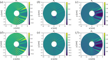
 $M=100$. Figure 3(a–c) shows the
 $(x,y,z)$ components of the time-averaged Poynting flux
 $\boldsymbol {S}$ exterior to the filament. The
 $\boldsymbol {S}$ is calculated using the relation
 $\boldsymbol {S} = ({1}/{2 \mu _0 \omega })\textrm {Im}\,{\boldsymbol {E}^{*} \times (\boldsymbol {\nabla } \times \boldsymbol {E})}$. The normalized field
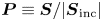 $\boldsymbol {P} \equiv {\boldsymbol {S}}/{|\boldsymbol {S}_{\textrm {inc}}|}$ is introduced, where
 $\boldsymbol {S}_{\textrm {inc}}$ is the Poynting flux of the incident wave. Figure 3 reveals a shadowing effect downstream of the filament. The striations in the field indicate strong back and side scattering of the incident wave. Note that
 $\boldsymbol {P}$ has been numerically computed from the interpolated
 $\boldsymbol {E}$-field on a grid in the
 $(x,y)$-plane. This method of plotting
 $\boldsymbol {P}$ is susceptible to large errors inside the filament where the gradients of
 $\boldsymbol {E}$ are large. Therefore,
 $\boldsymbol {P}$ inside the filament is not plotted.
Gaussian filament: normalized Poynting flux computed using the SAS model (a–c) and PETRA-M (d–f), where  $n_0=1\times 10^{19} \ \text {m}^{-3}$,
 ${B}=4 \ \text {T}$,
 $f=4.6\ \text {GHz}$,
 $N_{||} =2$,
 $n_b/n_0 = 4.8$, and
 $a_b=1\ \text {cm}$.

Figure 3(d–f) shows this case repeated in PETRA-M, and result in an excellent agreement with the SAS model. This 2-D simulation is done in a circular domain. The incident wave is excited to the left of the filament using an external current source term. To approximate an infinite background plasma, a perfectly matched layer (PML) is modelled at the perimeter of the circular simulation domain.
6.2. Reflection coefficient for turbulent slab
Next, the MC step of the SAS-MC model is compared with a turbulent slab modelled in PETRA-M. This will reveal whether the far-field limit, a critical approximation in the MC model, is valid for the treatment of LH scattering in the SOL. In theory, the far-field approximation should break down as filaments are packed closer together (Mishchenko Reference Mishchenko2014).
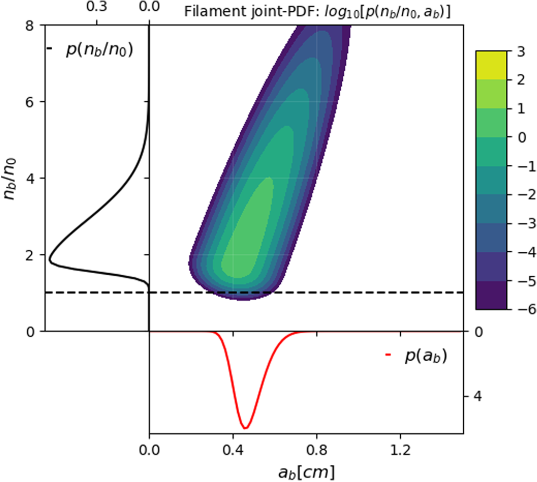
For the MC model,  $\sigma _{\text {eff}}(\theta )$ must be calculated, which first requires prescribing a joint-p.d.f. of filaments. Figure 4 plots an example joint-p.d.f. A bivariate skewed-normal distribution is assumed for
 $a_b$ and
 $n_b/n_0$ (see (4.6)). In this case,
 $\langle a_b \rangle = 0.48\ \textrm {cm}$ and
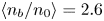 $\langle n_b/n_0 \rangle = 2.6$. These values are bounded by experimental SOL measurements (Zweben et al. Reference Zweben, Stotler, Terry, LaBombard, Greenwald, Muterspaugh, Pitcher, Group, Hallatschek and Maqueda2002; Terry et al. Reference Terry, Zweben, Hallatschek, LaBombard, Maqueda, Bai, Boswell, Greenwald, Kopon and Nevins2003). (Assuming SOL turbulence is predominantly filamentary, the approximation
 $\langle n_b/n_0 \rangle \approx 1 + ({n_{\text {RMS}}}/{n})f_{p}^{-1}$ is made, where
 $f_{p}$ is the packing fraction and is assumed to be
 $0.2$.) Filament relative density and size skewness are prescribed via the skewness parameters:
 $\boldsymbol{\varGamma} = [7,10]$. Filament relative density and size standard deviation are prescribed as
 $\boldsymbol{s} = [1.35, 0.1\ \text {cm}]$. The bivariate correlation coefficient
 $\eta =0.9$.
Example joint-p.d.f. of filament parameters  $n_b/n_0$ and
 $a_b$. A bivariate skewed-normal distribution is assumed (see (4.6)), where
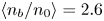 $\langle n_b/n_0 \rangle = 2.6$ and
 $\langle a_b \rangle = 0.48\,$cm. Filament density and size skewness
 $\boldsymbol{\varGamma} = [7,10]$. Filament density and standard deviation
 $\boldsymbol{s}=[1.35, 0.1\ \text {cm}]$. Correlation coefficient
 $\eta =0.9$. Dashed black line denotes
 $n_b/n_0 =1$.

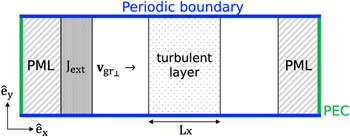
Figure 5 shows the simulation set-up for a slab turbulent geometry in PETRA-M. A slow wave travelling in the  $+x$-direction interacts with a turbulent layer populated with Gaussian filaments. The filaments are randomly generated in the slab using a Monte Carlo approach (Sierchio et al. Reference Sierchio, Cziegler, Terry, White and Zweben2016; Biswas et al. Reference Biswas, Baek, Bonoli, Shiraiwa, Wallace and White2020). Each filament is generated with a randomly picked
 $n_b/n_0$ and
 $a_b$ with a probability that satisfies the prescribed joint-p.d.f.
 $p(n_b/n_0, a_b)$. In this way, the turbulent slab used in the SAS-MC model and in PETRA-M are made statistically equivalent. The incident slow wave is excited with an external current density source function upstream of the turbulence. Top and bottom boundaries are periodic. The turbulence is also periodic in the
 $y$-direction. To minimize the effect of the periodic geometry on the wave, the
 $y$ length of the solution domain is much larger than
 $\langle a_b \rangle$ or
 $k_{\textrm {inc}\perp }$. To mimic an infinite domain in the
 $\pm x$-direction, the left and right boundaries can be modelled as either a perfectly matched layer (PML) or an absorbing boundary condition (ABC). The PML, while more computationally efficient, does not work when both the slow and fast wave can propagate in the background plasma.
Set-up for PETRA-M simulation with turbulent slab. Here, ‘PML’ denotes perfectly matched layer and ‘PEC’ denotes perfect electric conductor.

In PETRA-M, the reflection coefficient  $F_{\text {ref}}=1-P_{x}/P_{x,0}$ is calculated and directly compared with the SAS-MC value. Here,
 $P_{x}$ is the
 $x$-component of the Poynting flux and
 $P_{x,0}$ is the ‘nominal’ value when no turbulence is present. In the SAS-MC model,
 $F_{\text {ref}}=\int P_{{R}}(\theta )\,\textrm {d}\theta$.
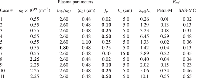
Table 1 compares  $F_{\text {ref}}$ computed in the PETRA-M and SAS-MC models. Both models follow the same general trend. Cases 1–4 and 8–11 reveal that
 $F_{\text {ref}}$ increases with
 $f_{p}$. Cases 3,5,6,8 reveal that
 $F_{\text {ref}}$ increases with
 $\langle n_b/n_0 \rangle$ and decreases with
 $\langle a_b \rangle$. This is consistent with previous scattering theories (Ott Reference Ott1979; Andrews & Perkins Reference Andrews and Perkins1983). Another way to analyse the trends in
 $F_{\text {ref}}$ between models is by inspecting
 $\varSigma _{\text {eff}}L_{x}$ calculated in the SAS-MC model. This is the attenuation factor for the ballistic power (see (5.3)). As
 $\varSigma _{\text {eff}}L_{x}$ increases, so should
 $F_{\text {ref}}$. Indeed, this is true for both models.
Comparison between SAS-MC model and PETRA-M. Slow wave launched at  $4.6\ \text {GHz}$ and
 $N_{||}=2$ with
 ${B}=4\ \text {T}$. Filament joint-p.d.f. parameters are same as in figure 4 unless otherwise noted. The
 $\varSigma _{\text {eff}}L_{x}$ is calculated using the SAS-MC model. For each case, results from multiple iterations (with different turbulence realizations) are averaged until
 $F_{\text {ref}}$ is statistically converged.

In general, the SAS-MC model over-predicts  $F_{\text {ref}}$, such that the absolute error
 $\Delta F_{\text {ref}} \equiv F_{\text {ref,SAS-MC}} - F_{\text {ref,PETRA-M}} \geq 0$. This error increases with
 $f_p$. Again, this arises from the far-field approximation breaking down. While far-field validity is dependent on
 $f_{p}$, the aggregate error depends on
 $\varSigma _{eff} L_{x}$. For example, the SOL width is varied between cases 2 and 7, while the turbulence is kept statistically identical. The
 $L_{x}=5\ \textrm {cm}$ case results in
 $\Delta F_{\text {ref}} = 0.00$. For the
 $L_{x}=15\ \textrm {cm}$ case,
 $\Delta F_{\text {ref}} = +0.13$.
SOL measurements indicate  $f_p \approx 0.05\text {--}0.25$ (Agostini et al. Reference Agostini, Zweben, Cavazzana, Scarin, Serianni, Maqueda and Stotler2007; Carralero et al. Reference Carralero, Artene, Bernert, Birkenmeier, Faitsch, Manz, de Marne, Stroth, Wischmeier and Wolfrum2018; Zweben et al. Reference Zweben, Terry, LaBombard, Agostini, Greenwald, Grulke, Hughes, D'Ippolito, Krasheninnikov and Myra2011). SOL widths are also
 ${<}5\ \textrm {cm}$ in present-day devices. As a result, cases 2 and 9 are most representative of a C-Mod SOL, depending on whether the background density is evaluated at the far-SOL or the separatrix, respectively. At low-density (case 2), the two models agree well (
 $\Delta F_{\text {ref}} = 0.00$). At high density (case 9), the SAS-MC model over-predicts
 $F_{\text {ref}}$, such that
 $\Delta F_{\text {ref}} = +0.08$. A possible reason for the disagreement at high density may be because
 $\varSigma _{\text {eff}}L_{x}$ is greater (compared with similar cases at low density).
6.3. Comments on computational cost
Generally, the semi-analytic scattering method has three key advantages compared with finite-element Maxwell solvers: (1) the large (in fact infinite) background plasma region does not need to be meshed; (2) it exactly solves scattering problems, because the infinite exterior domain does not need to be artificially truncated; (3) analysing the scattered wave spectrum is straight-forward, because the solution is already deconvolved into the constituent poloidal mode numbers for each branch.
Points 1 and 2 result in the SAS-MC model being considerably less expensive than slab turbulence simulations in PETRA-M. Using the SAS technique, computing a single differential scattering width  $\sigma (\theta ;n_b/n_0, a_b )$ takes
 ${\sim }10\ \textrm {s}$ on a single CPU, and considerably less time if parallelized between poloidal mode numbers. Computing
 $\sigma _{\text {eff}}(\theta )$ may require sampling a few hundred combinations of
 $(n_b/n_0, a_b)$, depending on the filament joint-p.d.f. Fortunately, each sampled
 $\sigma (\theta ;n_b/n_0, a_b )$ needs to be computed only once. Any number of
 $\sigma _{\text {eff}}(\theta )$ can then be generated from the sampled differential scattering widths.
The most expensive process in the MC routine is generating the transition matrix T. This takes  ${\sim }20\ \textrm {s}$ on a single CPU, depending on poloidal and radial bin resolution.
Using PETRA-M, each  $n_0 = 2.25 \times 10^{19}\ \text {m}^{-3}$,
 $L_{x} = 5\ \textrm {cm}$ slab case required
 ${\sim }25$ CPU-hours and
 ${\sim }300\ \textrm {GB}$ of RAM on the MIT Engaging computing cluster. The size of PETRA-M simulations is primarily limited by available RAM. In comparison, all computations for the SAS-MC model were conducted on a PC with 8 GB of available RAM.
6.4. Caveats to the SAS-MC model
The SAS-MC model offers higher physics fidelity than ray tracing, while being computationally less expensive than numeric full-wave solvers. This is possible owing to a number of assumptions made in the model that makes it less universally applicable than numeric full-wave solvers.
The SAS model assumes a homogeneous background plasma with a cylindrical scattering object (the filament) that is poloidally and azimuthally symmetric. This allows an efficient solution scheme using separation of variables. In reality, filaments usually develop a shock front as they convect outward (Krasheninnikov et al. Reference Krasheninnikov, D'Ippolito and Myra2008), and the resulting crescent-like filament shape can lead to significantly modified scattering behaviour, at least for ion cyclotron waves (Tierens, Zhang & Manz Reference Tierens, Zhang and Manz2020a). Furthermore, the filament in the SAS model is assumed to be aligned with the magnetic field, so that 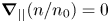 $\boldsymbol {\nabla }_{||} ( {n}/{n_0} )=0$. This is likely a reasonable assumption because filaments introduce a
 $\boldsymbol {\nabla }_{||} ( {n}/{n_0} )$ that is much smaller than
 $k_{||}$ of the LH wave (Grulke et al. Reference Grulke, Terry, Cziegler, LaBombard and Garcia2014). As a result, the effect of
 $k_{||}$ broadening arising from a typical SOL filament is small (Madi et al. Reference Madi, Peysson, Decker and Kabalan2015).
The MC model introduces additional assumptions. The SOL is treated as a slab, which means the effect of toroidal geometry is neglected. This is a reasonable assumption for the treatment of first-pass scattering in front of the antenna. In addition, the background plasma and turbulence parameters are constant within the slab, when in reality, they are sensitive to the radial coordinate in a tokamak. The MC model also assumes the reflected wave spectrum is lost, when in reality, a fraction of this power may once again reflect at a cutoff and re-enter the core plasma. Lastly, the MC model assumes the filaments are far enough apart so that the RTE is valid. This assumption is increasingly poor as  $f_p$ rises.
To quantify the inaccuracies introduced by the MC model, it may be worthwhile to model scattering along the full extent of a ray trajectory in a realistic tokamak geometry. This can be done by employing  $\sigma (\theta ; n_0, B, N_{||}, \langle n_b/n_0 \rangle, \langle a_b \rangle )$ as a scattering probability in a Monte Carlo ray tracing simulation, similar to what has been done for the
 $k$-scattering model (Bonoli & Ott Reference Bonoli and Ott1982; Bertelli et al. Reference Bertelli, Wallace, Bonoli, Harvey, Smirnov, Baek, Parker, Phillips, Valeo and Wilson2013). Alternatively, three-dimensional (3-D) PETRA-M simulations of LH launching in a turbulent SOL, with realistic geometry, would address all the caveats mentioned. These tests are outside the scope of this paper.
7. SAS-MC applied to lower hybrid scattering
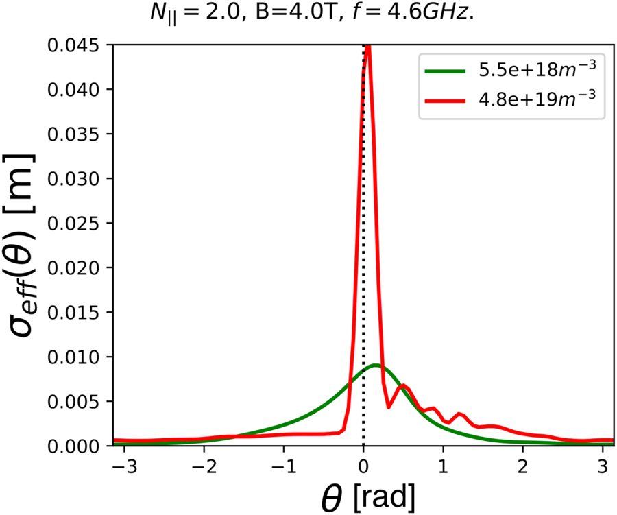
The SAS-MC model is applied to LH wave scattering in front of the antenna in C-Mod. Figure 6 plots  $\sigma _{\text {eff}} (\theta )$ for the joint-p.d.f. in figure 4, and
 $N_{||}=2$,
 $f=4.6\ \text {GHz}$ and
 ${B}=4\ \text {T}$. At low background density (
 $n_0 = 5.5 \times 10^{18}\ \text {m}^{-3}$),
 $\sigma _{\text {eff}} (\theta )$ resembles a wrapped-Cauchy distribution, though slightly skewed so that it peaks at
 $+0.2\ \text {rad}$. At high background density (
 $n_0 = 4.8 \times 10^{19}\ \text {m}^{-3}$),
 $\sigma _{\text {eff}} (\theta )$ is sharply peaked near
 $+0.05\ \text {rad}$ and is very asymmetric. A fat tail exists only for
 $\theta > 0$. This tail also has fine structures that do not exist in the low density case. The
 $\sigma _{\text {eff}} (\theta )$ is more asymmetric at higher densities because
 $|\varepsilon _{xy}|$ is larger, and therefore the effect of asymmetric scattering for any given filament is stronger (see § 7.2 for more details).
Effective differential scattering width  $\sigma _{\text {eff}} (\theta )$. Calculated using filament joint-p.d.f. shown in figure 4. Green and red lines denote low and high background density, respectively.

7.1. Parametric scan of SOL density and filament parameters
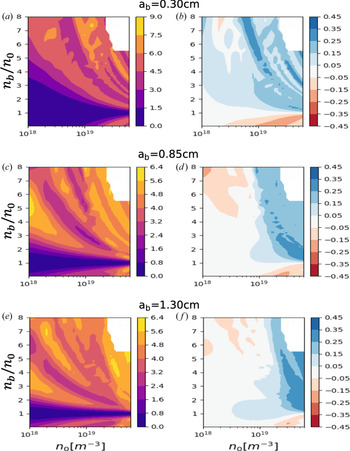
Figure 7(a,c,e) plots  $\sigma _{S}$ as a function of background density
 $n_0$, relative filament density
 $n_b/n_0$ and filament width
 $a_b$. The incident wave is at 4.6 GHz with
 $N_{||}=2$, typical for LH launching in C-Mod. In accordance with the low-field-side SOL in C-Mod,
 ${B}=4\ \text {T}$. As expected,
 $\sigma _{S}$ increases as
 $n_b/n_0$ deviates from unity. Notably, scattering resonances can be seen, as indicated by bands of higher
 $\sigma _{S}$. These arise from standing wave resonances excited within the filament, which result in stronger coupling to the scattered waves. Expressions for these resonances can be analytically derived for the ‘flat-top’ filament case (Myra & D'Ippolito Reference Myra and D'Ippolito2010; Tierens et al. Reference Tierens, Zhang and Myra2020b), and are related to radial and poloidal harmonics in cylindrical geometry. To the best of the authors’ knowledge, these analytic calculations are intractable for Gaussian (and more general) filament cross-sections.
Plots of (a) scattering width  $\sigma _{S}$ and (b) asymmetric scattering metric
 $\alpha$ for an incident slow wave at 4.6 GHz,
 $N_{||}=2$,
 ${B}=4\ \text {T}$ and
 $a_b =0.30\ \text {cm}$. (c,d) Plot of
 $\sigma _{S}$ and
 $\alpha$, respectively, for
 $a_b=0.85\ \text {cm}$. (e,f) Plot of
 $\sigma _{S}$ and
 $\alpha$, respectively, for
 $a_b=1.30\ \text {cm}$. The white region in the upper-right corner of each subplot has no data plotted.

7.2. Asymmetric scattering
The quantity  $\alpha$ is introduced as a metric for asymmetric scattering:
 \begin{equation} \alpha = \int_{0}^{\rm \pi} \hat{\sigma}_{S}(\theta) \,\textrm{d} \theta - \tfrac{1}{2}. \end{equation}
Here  $\alpha =-0.5,+0.5$ denote that power is only scattered downwards (
 $-{\rm \pi} < \theta < 0$), upwards (
 $0 < \theta < {\rm \pi}$). If
 $\alpha =0$, then an equal fraction of power is scattered downwards and upwards. Figure 7(b,d,f) reveals that
 $\alpha$ is not guaranteed to be zero. This means, in general,
 $\sigma (\theta )$ is not an even function and the scattered power is not equally distributed downwards or upwards. This effect is most noticeable at high background densities (
 $n_0 \gtrsim 2\times 10^{19}\ \text {m}^{-3}$). For positive density modifications (
 $n_b/n_0 > 1$), power is predominantly scattered upwards. The reverse is true for negative density modifications (
 $n_b/n_0 < 1$). In the typical tokamak SOL, filaments are predominantly denser than the background plasma (Graves et al. Reference Graves, Horacek, Pitts and Hopcraft2005). As a result, the incident wave is preferentially scattered upwards. The strength of this asymmetry depends on the statistical properties of the filaments.
Asymmetric scattering is possible in an anisotropic medium. Specifically, the dielectric dyadic tensor,  $\varepsilon$, has off-diagonal components
 $\varepsilon _{12} = -\varepsilon _{21} \neq 0$, which permit asymmetric scattering (Wu Reference Wu1994), so
 $\varepsilon _{12}=-\textrm {i} \varepsilon _{xy}$. In the LH limit,
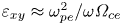 $\varepsilon _{xy}\approx \omega _{pe}^{2}/{\omega \varOmega _{ce}}$, where
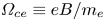 $\varOmega _{ce} \equiv eB/m_e$ is the electron cyclotron frequency. It is clear that the sign of
 $\varepsilon _{xy}$ is dependent on the sign of
 $B$ (that is, whether the magnetic field is oriented co-parallel or counter-parallel with
 $\hat {e}_{z}$). Correspondingly, when the direction of
 $\boldsymbol {B}$ is flipped,
 $\boldsymbol{\varepsilon} \rightarrow \boldsymbol{\varepsilon}^{T}$ and
 $\sigma (\theta ) \rightarrow \sigma (-\theta )$.
Notably, this asymmetric scattering effect is not accounted for in previous treatments for LH wave scatter. It is easy to see why this is the case for models that assume drift-wave-like turbulence. These models assume that density fluctuations are equally likely to be above or below the background density. Therefore, this asymmetric scatter effect is statistically cancelled out.
There also exist LH scattering models that assume coherent turbulent structures that can, on average, be denser than the background (Hizanidis et al. Reference Hizanidis, Ram, Kominis and Tsironis2010; Biswas et al. Reference Biswas, Baek, Bonoli, Shiraiwa, Wallace and White2020). These models also do not account for asymmetric scattering, because they make the ray tracing approximation.
The reason why ray tracing cannot model asymmetric scattering is subtle. It is related to the breakdown of the ray tracing approximation. Consider the ray tracing equations for an LH ray initially propagating with  $\boldsymbol {N}_{\perp }$ aligned along the
 $x$-direction and background
 $\boldsymbol {B}$ aligned along the
 $z$-direction. The ray tracing equations involve partial derivatives of
 $\text {det}(\boldsymbol {D})$, where
 $\boldsymbol {D}$ is now the dielectric tensor and
 \begin{equation} \boldsymbol{D} \boldsymbol{\cdot} \tilde{\boldsymbol{E}}= \begin{bmatrix} \varepsilon_{{\perp}} - N_{||}^{2} & -\textrm{i}\varepsilon_{xy} & N_{{\perp}}N_{||} \\ i\varepsilon_{xy} & \varepsilon_{{\perp}} - N^{2} & 0 \\ N_{{\perp}}N_{||} & 0 & \varepsilon_{||} - N_{{\perp}}^{2} \end{bmatrix} \boldsymbol{\cdot} \begin{bmatrix} \widetilde{E_x} \\ \widetilde{E_y} \\ \widetilde{E_z} \end{bmatrix} = 0,\end{equation}
where  $\tilde {\boldsymbol {E}}(\boldsymbol {r})$ is the slowly varying part of the electric field. Here, det(
 $\boldsymbol {D}$) has terms that are quadratic in
 $\varepsilon _{xy}$, but no linear
 $\varepsilon _{xy}$ terms. As a result, information about the sign of
 $B$ along
 $\hat {e}_{z}$ is lost. Compare this to the full EM wave equation, with no ray tracing approximation, written in a form similar to that of (7.2).
 \begin{equation} \begin{bmatrix} \varepsilon_{{\perp}} - \dfrac{c^{2}}{\omega^{2}}(F_{yy} + F_{zz}) & \dfrac{c^{2}}{\omega^{2}}F_{yx} - \textrm{i}\varepsilon_{xy} & \dfrac{c^{2}}{\omega^{2}}F_{zx}\\ \dfrac{c^{2}}{\omega^{2}}F_{xy} + \textrm{i}\varepsilon_{xy} & \varepsilon_{{\perp}} - \dfrac{c^{2}}{\omega^{2}}(F_{zz} + F_{xx}) & \dfrac{c^{2}}{\omega^{2}}F_{zy}\\ \dfrac{c^{2}}{\omega^{2}}F_{xz} & \dfrac{c^{2}}{\omega^{2}}F_{yz} & \varepsilon_{||} - \dfrac{c^{2}}{\omega^{2}}(F_{xx} + F_{yy}) \end{bmatrix} \boldsymbol{\cdot} \begin{bmatrix} \widetilde{E_x} \\ \widetilde{E_y} \\ \widetilde{E_z} \end{bmatrix} = 0,\end{equation}
where
 $$\begin{gather} F_j = k_j - \textrm{i} \frac{\partial}{\partial j} , \end{gather}$$
 $$\begin{gather}F_{jl} = F_j(F_l). \end{gather}$$
Equation (7.3) accounts for  $\boldsymbol {\nabla } \boldsymbol {k}$ and
 $\boldsymbol {\nabla } \tilde {\boldsymbol {E}}$ terms, which are usually neglected in ray tracing because the plasma is assumed to be sufficiently homogeneous, such that
 $k_{\perp }L_n \gg 1$, where
 $L_n\equiv |{\boldsymbol {\nabla } n}/{n_0}|^{-1}$ is the characteristic length of the density inhomogeneity. This heuristic validity criterion is actually too lax for magnetized plasma. A perturbation analysis of (7.3) reveals that these higher-order gradient terms can be comparable to the zeroth-order terms (7.2) even if
 $k_{\perp }L_n \gg 1$. Following some algebra, it is found that the two leading higher-order terms are linear in
 $\varepsilon _{xy}$ and quadratic in
 $N_{||}$, such that the actual validity criterion for ray tracing is
 $(|\varepsilon _{xy}| + N_{||}^{2}) {1}/{k_{\perp } L_{n}} \ll 1$. (More details about this perturbation analysis can be found in Appendix A of Biswas et al. (Reference Biswas, Baek, Bonoli, Shiraiwa, Wallace and White2020), although in that derivation,
 $\boldsymbol {\nabla }\boldsymbol {k}$ terms were erroneously neglected, which led to the dropping of the
 $N_{||}^{2}$ term in the final ray tracing validity criterion.) At initial launching of the LH wave
 $N_{||}^{2} , |\varepsilon _{xy}| \sim 1$, but they can both grow to be much larger as the ray continues to propagate. Specifically,
 $|\varepsilon _{xy}|\propto n_e$, and so it rapidly increases as the ray propagates into the plasma. The restriction that
 $\varepsilon _{xy}$ places on LH ray tracing has been commented on before (Ott Reference Ott1979). The following discussion is the first time it has been linked to asymmetric scattering in the context of LH waves.
In deriving the new ray tracing criterion for LH waves in a magnetized plasma, it was revealed that one of the leading higher-order gradient terms neglected in ray tracing is linear in  $\varepsilon _{xy}$. This is precisely the term with information about the orientation of
 $\boldsymbol {B}$. In accordance, as
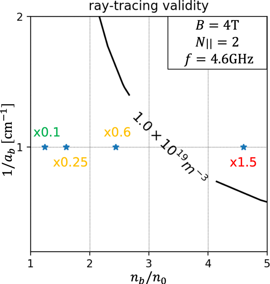
 $|\varepsilon _{xy}|{1}/{k_{\perp } L_n}$ grows and becomes comparable to unity, asymmetric scattering also becomes important. This is shown numerically by simulating the scatter of LH waves from four increasingly dense Gaussian filaments. Figure 8 plots the validity regime of ray tracing in the presence of a Gaussian filament as a function of
 $n_b/n_0$ and
 $a_b$. The incident wave is launched at 4.6 GHz with
 $N_{||}=2$ and
 ${B} = 4\ \text {T}$. It is assumed that
 $L_{n}^{-1} \approx ({n_b}/{n_0}-1)/a_b$. The black line denotes the validity limit for
 $n_0 = 1 \times 10^{19}\ \text {m}^{-3}$. To the right of this line,
 $|\varepsilon _{xy}|{1}/{k_{\perp } L_n} > 1$ and to the left
 $|\varepsilon _{xy}|{1}/{k_{\perp } L_n} < 1$. (For simplicity, the
 $N_{||}^{2}$ term is ignored.) The four starred points denote filaments with
 $a_b = 1$ cm and
 $n_b/n_0 = [1.24, 1.6, 2.44, 4.6]$ (plotted left to right). Alternatively, these filaments satisfy
 $n_b = [0.1, 0.25, 0.6, 1.5]\times n_{b,\text {max}}$, where
 $n_{b,\text {max}}$ satisfies
 $|\varepsilon _{xy}|{1}/{k_{\perp } L_n} = 1$. Qualitatively, the green point signifies a filament that is validly treated with ray tracing because
 $|\varepsilon _{xy}|{1}/{k_{\perp } L_n} \approx {n_b}/{n_{b,\text {max}}} = 0.1 < 1$. The yellow points are marginally valid, because
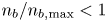 ${n_b}/{n_{b,\text {max}}} < 1$ but also
 $\mathscr {O}(1)$. The red point, for which
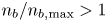 ${n_b}/{n_{b,\text {max}}} > 1$, certainly cannot be treated using ray tracing.
Validity of ray tracing for Gaussian filaments as a function of relative density ( $n_b/n_0$) and radial width (
 $a_b$). Black line denotes validity limit at
 $n_0 = 1 \times 10^{19}\ \text {m}^{-3}$ (see § 7.2 for more details). Stars denote filaments that are used in scattering studies in figures 9 and 10. Numbers in colour denote the ratio
 $n_b/n_{b,\text {max}}$.

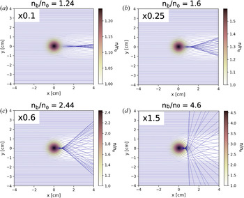
Figure 9 plots the ray trajectories of LH rays incident from the left and interacting with a filament. As  $n_b/n_0$ increases, rays are more strongly refracted, which results in a shadowing effect downstream of the filament. Notably, these ray trajectories are always perfectly symmetric with respect to
 $y=0$.
Ray tracing simulations of LH waves scattering from a filament. Here,  $f=4.6\ \textrm {GHz}$,
 $N_{||}=2$,
 ${B}=4\ \text {T}$ and
 $n_0 = 1 \times 10^{19}\ \text {m}^{-3}$. Each subplot corresponds to a star on figure 8. Blue lines denote ray trajectories.

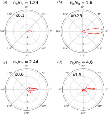
In contrast, figure 10 plots  $\sigma (\theta )$ calculated using the SAS method for the same four cases simulated in figure 9. The SAS method (like all full-wave treatments) implicitly accounts for all terms in (7.3). For
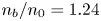 $n_b/n_0=1.24$ and 1.6,
 $\sigma (\theta )$ is symmetric about
 $\theta = 0$. The profiles peak at
 $\theta =0$, signifying predominantly forward scatter. At
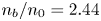 $n_b/n_0=2.44$,
 $\sigma (\theta )$ is slightly asymmetric because the side lobe at
 $-40^{\circ }$ is larger than the one at
 $+40^{\circ }$. At
 $n_b/n_0=4.6$,
 $\sigma (\theta )$ is clearly asymmetric. Notably, the largest lobe is centred at
 $+5^{\circ }$. While a direct quantitative comparison between figures 9 and 10 is not possible, it is clear that as
 $|\varepsilon _{xy}|{1}/{k_{\perp } L}$ grows (filaments get denser), ray tracing becomes less accurate because the increasingly important asymmetric scattering effect is ignored. It is important to note that filaments with
 $n_b/n_0 \gtrsim 2$ are common in the SOL (Zweben et al. Reference Zweben, Stotler, Terry, LaBombard, Greenwald, Muterspaugh, Pitcher, Group, Hallatschek and Maqueda2002), which signifies ray tracing is inadequate for the treatment of LH wave scattering in realistic SOL turbulence.
Polar plots of differential scattering width  $\sigma (\theta )$ calculated using the SAS method. Simulation parameters are the same as in figure 9.

7.3. Modified wave spectrum in front of LH antenna
The incident wave parameters, background plasma parameters and joint-p.d.f. of filament parameters determine  $\sigma _{\text {eff}}(\theta )$. The MC method is used to compute the modified wave spectrum after the incident wave interacts with a slab layer of thickness
 $L_{x}$ and packing fraction
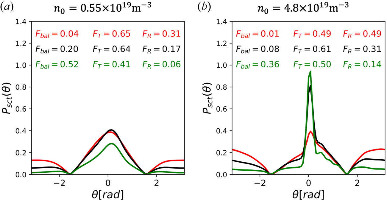
 $f_p$. Figure 11 plots the modified wave spectra resulting from the
 $\sigma _{\text {eff}}(\theta )$ shown in figure 6. Here,
 $L_{x} = 2.5\ \textrm {cm}$, which is the typical gap between the LH antenna and the separatrix in C-Mod. Green, black and red lines denote
 $f_p=[0.1,0.25,0.5]$. Note that the ballistic power fraction is not plotted (if it were, it would be a Dirac delta plotted at
 $\theta = 0$). In the low-density (
 $n_0 = 0.55 \times 10^{19}\ \text {m}^{-3}$) case, the modified wave spectrum is smoothly broadened in
 $\theta$-space, with a peak centred at
 $\theta = 0$. Increase in
 $f_p$ leads to a decrease in ballistic power and increase in reflected power. This is expected, because
 $\varSigma _{\text {eff}}$, the inverse mean-free-path to scatter, is linearly proportional to
 $f_p$. In the high-density (
 $n_0 = 4.8 \times 10^{19}\ \text {m}^{-3}$) case, the modified wave spectrum is significantly asymmetric, with net power scattered in the
 $+\theta$-direction. Naturally, this is the result of
 $\sigma _{\text {eff}}(\theta )$ in the high-density case being very asymmetric. Again, ballistic power decreases and reflected power increases with
 $f_p$. In comparing the low- and high-density cases, it is found that the high-density case results in significantly greater reflected power. This arises from
 $\sigma _{\text {eff}}$ being larger in the high-density cases, as can be seen from figure 6.
Modified LH wave spectrum after interacting with turbulent slab. Here,  $|\theta | < {\rm \pi}/2$ denotes transmitted power and
 $|\theta | > {\rm \pi}/2$ denotes reflected power. Ballistic power is not plotted and
 $f_p =$ 0.1 (green), 0.25 (black), 0.5 (red). Left and right plots assume low and high background density, respectively. The
 $F_{\text {bal}}$,
 $F_{{T}}$ and
 $F_{{R}}$ denote fractional ballistic, transmitted and reflected power, respectively. The
 $\sigma _{\text {eff}}(\theta )$ used is shown in figure 6.

7.4. SAS-MC compared with ray tracing
A comparison study between the SAS-MC model and ray tracing model is conducted. Rays are launched in a slab geometry and are incident normal to a slab composed of randomly generated filaments (see § 6.2). A ray terminates when it leaves the slab (either reflected backward or transmitted forward), at which point the angle between the ray's perpendicular group velocity ( $\boldsymbol {v}_{gr_{\perp }}$) and
 $\hat {e}_x$ is tallied. This poloidal angle is the direction that the ray continues to propagate and radiate power away from the slab. It is therefore equivalent to
 $\theta$ in the SAS-MC model. Following multiple ray launches, a histogram of these tallies is constructed. This histogram, once properly normalized, is equivalent to a modified wave spectrum that can be compared with the wave spectrum computed with the SAS-MC model.
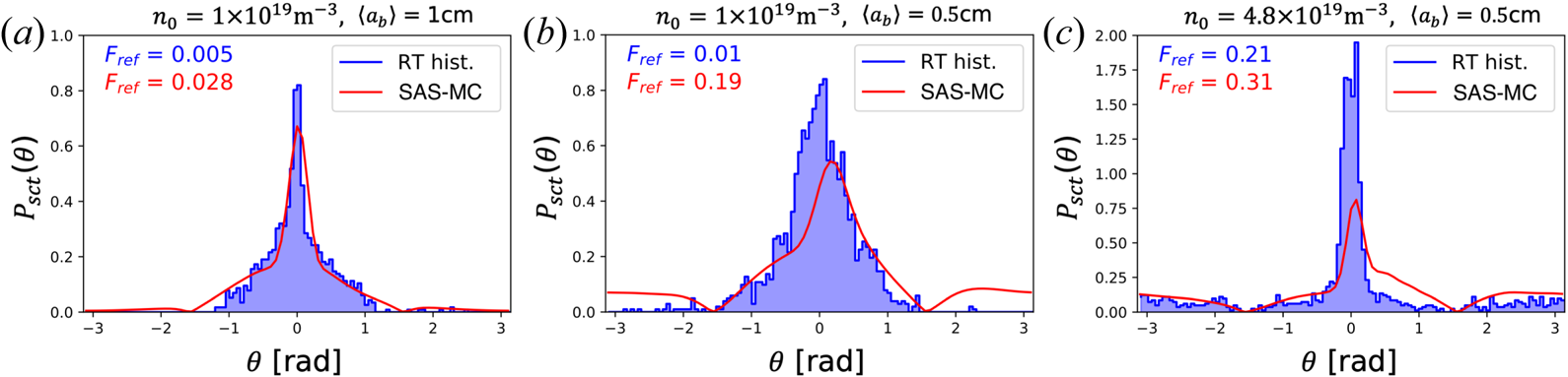
Figure 12 plots modified wave spectra computed using the SAS-MC model and the ray tracing model for statistically identical turbulent slabs. Three different cases are run. All cases assume LH rays incident at 4.6 GHz and  $N_{||}=2$. Here,
 ${B}=4\ \text {T}$ and
 $L_x=2.5\ \textrm {cm}$. In the first case,
 $n_0 = 1 \times 10^{19}\ \text {m}^{-3}$, and the joint-p.d.f. in figure 4 is assumed. The SAS-MC model and ray tracing model show good agreement in the wave spectra. Both predict low reflected power fractions. The wave spectrum computed with the SAS-MC model is fairly symmetric. This means that asymmetric scatter was weak, and therefore the ray tracing approximation was valid. Thus, the good agreement between the two models. In the next case,
 $\langle a_b \rangle$ is halved to 0.5 cm. The SAS-MC model results in an asymmetric wave spectrum, such that the peak is shifted to
 $+0.2$ rad. The onset of significant asymmetric scattering is caused by the decrease in
 $L_{n}$. At the same time, the ray tracing approximation begins to break down. As a result, the ray tracing results (which are symmetric) begin to deviate from the SAS-MC results. Notably, the ray tracing model severely under-predicts the fraction of reflected power compared with the SAS-MC model. The last case increases the background density to
 $n_0 = 4.8 \times 10^{19}\ \text {m}^{-3}$. Now,
 $\varepsilon _{xy}$ is large enough that asymmetric scattering is quite strong and the ray tracing approximation is surely invalid. As a result, the two models result in very different wave spectra. Ray tracing predicts a scattered wave spectrum with a large central peak at
 $\pm 0.2\ \textrm {rad}$. In contrast, the SAS-MC model predicts a smaller central peak slightly shifted in the
 $+\theta$-direction. The tail to the right of this peak is significantly larger than the one on the left. Lastly, the SAS-MC model results in
 $\sim$50 % more power being reflected than the ray tracing model.
Comparison between the SAS-MC and ray tracing slab models. Blue bars denote a histogram of ray  $\boldsymbol {v}_{gr_{\perp }}$ angles after leaving slab. Red line denotes a modified wave spectrum
 $P_{sct} (\theta )$ calculated using the SAS-MC method. Here,
 $L_x = 2.5\ \textrm {cm}$ and
 $f_p = 0.25$. Filament joint-p.d.f. parameters are the same as in figure 4 unless otherwise noted in the subplot title. The
 $F_{\text {ref}}$ denotes fractional power reflected in the ray tracing (blue) and SAS-MC (red) models. Ballistic power and unscattered rays are not plotted.

8. Impact of scattering on LHCD
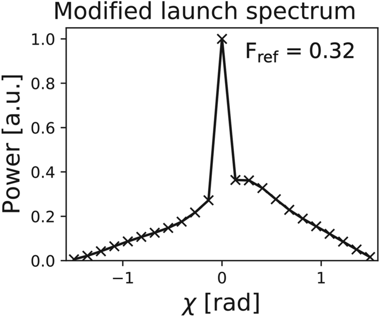
In typical ray tracing/Fokker–Planck simulations, the initial perpendicular wave vector  $\boldsymbol {k}_{\perp }$ of the slow wave is assumed co-parallel with the unit vector normal to the flux surface and pointing outwards (
 $\hat {e}_{\boldsymbol {\nabla } \psi }$). Therefore, the angle between these two vectors,
 $\chi \equiv \angle (\hat {e}_{\boldsymbol {\nabla } \psi },\boldsymbol {k}_{\perp })$, is usually zero. Scattering caused by edge density fluctuations can rotate
 $\boldsymbol {k}_{\perp }$ leading to a broadened wave spectrum in
 $\chi$-space, as evidenced by the LH electric field vector measurements in C-Mod (Martin et al. Reference Martin, Lau, Wallace, Shiraiwa and Mumgaard2019). This rotation can modify the ray path so that single-pass damping is strengthened or weakened, depending on the sign of
 $\chi$ (Baek et al. Reference Baek, Biswas, Bonoli, Brunner, Faust, Hubbard, Hughes, LaBombard, Mumgaard and Porkolab2020).
The  $\chi$ angle in the tokamak frame and
 $\theta$ in the slab geometry (as defined in figure 1) are identical if
 $\chi$ is defined such that
 $\hat {{b}} \boldsymbol {\cdot } (\hat {e}_{\boldsymbol {\nabla } \psi } \times \boldsymbol {k}_{\perp }) = k_{\perp } \sin {\chi }$, where
 $\hat {{b}} = \boldsymbol {B}/ |{B}|$ is the local magnetic field unit vector.
Thus, the transmitted wave spectrum calculated using the SAS-MC model can be coupled to GENRAY/CQL3D to study its impact on LHCD. A  $\chi$-broadened wave spectrum can be discretized into rays with initial wave-vector components as follows (Smirnov & Harvey Reference Smirnov and Harvey2001):
 $$\begin{gather} k_{\rho} = k_{{\perp}} \cos{\chi}, \end{gather}$$
 $$\begin{gather}k_{\theta} = k_{||} \frac{B_{\theta}}{B} - k_{{\perp}} \sin{\chi} \frac{B_{\phi}}{B}, \end{gather}$$
 $$\begin{gather}k_{\phi} = k_{||} \frac{B_{\phi}}{B} + k_{{\perp}} \sin{\chi} \frac{B_{\theta}}{B}, \end{gather}$$
where  $\rho$,
 $\theta$ and
 $\phi$ are now the radial, poloidal and toroidal coordinates in a toroidal coordinate system. Here,
 $B_{\rho }$ is neglected so that
 $\hat {e}_{\boldsymbol {\nabla } \psi } \approx \hat {e}_{\rho }$. In the above expression, it is assumed that
 $k_{\perp }>0$, while
 $\text {sign}(k_{\parallel })$ depends on whether the ray is launched with a positive or negative component with respect to
 $\hat {{b}}$. Next, consider that to drive co-current via electron Landau damping, it is required that
 $\text {sign}(k_{\parallel })=\text {sign}(B_{\phi }B_{\theta })$. Notably, this leads to rays with
 $\chi > 0$ being rotated away from the core. Conversely, rays with
 $\chi <0$ are rotated towards the core. This is true in all tokamak orientations, regardless of toroidal magnetic field or current direction.
A well-studied (Mumgaard Reference Mumgaard2015), low-density, L-mode discharge is modelled. This upper single-null discharge, with  $\bar {n}_e = 0.52 \times 10^{20}\ \text {m}^{-3}$,
 $I_p = 530\ \textrm {kA}$ and
 ${B}=5.4\ \textrm {T}$, achieves non-inductive current drive using 850 kW of LH power launched at 4.6 GHz with
 $N_{||} = -1.6$. (
 $\bar {n}_e$ is line-averaged electron density and
 $I_p$ is plasma current.) It is assumed that
 $85\,\%$ of power is coupled to the primary lobe. In GENRAY, this primary lobe is centred at
 $N_{||}=-1.6$, and is discretized into 12 bins in
 $N_{||}$-space. Each bin is further discretized into 23 rays to model wave-spectrum broadening in
 $\chi$-space. Figure 13 plots the SAS-MC-calculated transmitted wave spectrum assuming SOL background density
 $n_0 = 1 \times 10^{19}\ \text {m}^{-3}$, SOL width
 $L_x = 2.5\ \textrm {cm}$ and packing fraction
 $f_{p}=0.25$. The filament joint-p.d.f. is the same as in figure 4. The spike at
 $\chi =0$ accounts for ballistic power. Note that the reflected power, which accounts for roughly
 $30\,\%$ of power in the primary lobe, is assumed lost and therefore not modelled in GENRAY. Lastly, the spatial height of the launcher is modelled as four poloidal points in the outer mid-plane. In total, 1104 rays are launched to ensure a converged solution.
Modified wave spectrum launched in GENRAY/CQL3D simulation of LHCD in Alcator C-Mod. Wave spectrum calculated using the SAS-MC model for slow wave launched at 4.6 GHz and  $N_{||}=1.6$. SOL background density
 $n_0 = 1 \times 10^{19}\ \text {m}^{-3}$, packing fraction
 $f_p = 0.25$ and SOL width
 $L_x = 2.5\ \textrm {cm}$ are assumed. Filament joint-p.d.f. parameters are the same as in figure 4. Crosses show discretization of wave spectrum into rays for use in GENRAY. Spike at
 $\chi =0$ arises from ballistic power. Reflected power is ignored.

The rays are launched from the separatrix, but are allowed to propagate into the SOL after the first pass. Here, the rays will either reflect at the cutoff density or specularly reflect from the vessel wall back towards the core. Owing to low temperatures in the SOL, collisional damping is non-negligible. It is found that the SOL topology and presence of a divertor can significantly affect the calculated core CD profiles. Therefore, the two-point model is used to accurately generate the SOL (Shiraiwa et al. Reference Shiraiwa, Baek, Faust, Wallace, Bonoli, Meneghini, Mumgaard, Parker, Scott and Harvey2015). Once the proper SOL geometry is set, parameters like SOL e-folding width and divertor temperature do not strongly affect the core CD results for cases with the  $\chi$-broadened wave spectrum.
Figure 14 plots the calculated core power deposition and CD profile in this C-Mod discharge. The core density is scaled by  $\pm 10\,\%$ to assess the sensitivity of these results. The top figures, for which the launched wave spectrum was not broadened in
 $\chi$-space, reveal core profiles that are robustly peaked at
 $\rho \approx 0.8$. A smaller peak exists on-axis, though it shifts to
 $\rho \approx 0.25$ when the background density is decreased by
 $-10\,\%$. A robust current valley exists at
 $\rho \approx 0.5$. The bottom plots model a launched wave spectrum that is
 $\chi$-broadened. These profiles are remarkably different from the cases without broadening. There is a
 $65\,\%$ increase in power deposited near-axis (
 $\rho < 0.5$), which leads to profiles that are robustly peaked on-axis. There are also no large off-axis peaks.
Core LH power deposition and driven current density profiles in C-Mod L-mode discharge #1101104011 at  $t=1.10\ \textrm {s}$, modelled with GENRAY/CQL3D. Here,
 $\overline {n_e} = 0.52\times 10^{20} \ \text {m}^{-3}$,
 $I_p = 530\ \text {kA}$ and
 ${B}=5.4\ \textrm {T}$. An LH power of
 $850\ \textrm {kW}$ is launched at 4.6 GHz and
 $N_{||}=1.6$. (a,b) Simulations with no wave spectrum broadening. (c,d) Simulations with the broadened angular wave spectrum shown in figure 13. Green, black and red lines denote the core background density is scaled x0.9, x1.0 and x1.1 the nominal value, respectively.

Figure 15 plots the cumulative CD profile. The  $\chi$-broadened cases result in roughly linear profiles and greater current driven near-axis. In contrast, the cases without broadening result in CD preferentially in the off-axis (
 $\rho > 0.7$) region. The total LH current is
 $10\text {--}20\,\%$ lower in the broadened cases. This is partly owing to
 ${\sim }30\,\%$ of incident power being reflected in the SAS-MC model, and therefore not being launched in GENRAY for the
 $\chi$-broadened cases.
Cumulative core LH current driven, modelled in GENRAY/CQL3D. Simulation parameters are the same as in figure 14.

Figure 16 plots the ray trajectories during the first pass. Ray colour denotes the logarithmic power in the ray, normalized to initial power in the highest-powered ray. In the case with no broadening, rays cannot propagate to the hot magnetic axis, and therefore cannot Landau damp strongly. In contrast,  $\chi$-broadening ‘fans’ out the initial ray trajectories. Notably, rays that are sufficiently rotated inwards (
 $\chi < 0$) strongly Landau damp in the hot near-axis plasma. Even though this is a small fraction of the incident power, it is sufficient to seed a supra-thermal electron tail near-axis. As a result, additional rays can quasi-linearly damp on this tail on subsequent passes through the core. In the case without broadening, there is insufficient on-axis power for this seeding effect. As a result, the on-axis current drive is relatively low.
Poloidal projection of first-pass ray trajectories in C-Mod discharge. Simulation parameters are the same as in figure 14 for the x1.0 scaled density case. Coloured lines denote ray trajectories. The colour of lines denotes the  $\text {log}_{10}$ power in ray, normalized to the initial power in highest-power ray. Grey patch denotes core region (
 $\rho < 1$). Green patch denotes near-axis region (
 $\rho < 0.2$).

Note that the modified wave spectrum has a net effect of deflecting power away from the core on first pass. Paradoxically, near-axis CD increases. Again, this is attributed to the small fraction of power deflected inwards that seeds a near-axis supra-thermal electron tail. It is possible this phenomenon does not extend to high-density discharges, where stronger asymmetric scattering will deflect a greater fraction of power outwards.
9. Conclusion
A hybrid semi-analytic scattering Markov chain (SAS-MC) model is formulated to calculate the modified wave spectrum of an RF wave propagating through a turbulent SOL. First, a semi-analytic full-wave technique is adopted to calculate the scattered power from a SOL filament. This technique is generalized to account for filaments with radially varying densities. Next, an effective differential scattering width is derived for a statistical ensemble of filaments. Lastly, the SOL is modelled as a slab, and the modified wave spectrum is found by solving the radiative transfer equation using a Markov chain technique. This model is applied to the case of lower hybrid launching for driving current in a tokamak. GENRAY/CQL3D is used to model the impact of the modified wave spectrum on current drive in Alcator C-Mod.
In calculating the differential scattering width, it is found that the scattered power can be asymmetrically directed (in the  $y$-direction). This is true even for the effective scattering width, which averages over the statistical properties of filaments. Previous RF scattering models have either used the drift-wave approximation and/or the ray tracing approximation. As a result, they fail to account for this important asymmetric effect.
The SAS-MC model is compared with the ray tracing treatment of LH wave scattering. By retaining full-wave effects, the SAS-MC model is able to produce a significantly asymmetric transmitted wave spectrum. As stated previously, ray tracing cannot replicate this effect.
The SAS-MC model is compared with PETRA-M, which self-consistently models full-wave interactions in the presence of multiple filaments. Both models predict that  $F_{\text {ref}}$ increases with
 $\langle n_b/n_0 \rangle$,
 $\langle a_b \rangle ^{-1}$ and
 $L_{x}$, as do previous analytic scattering models. Assuming a low background density, and realistic SOL packing fraction and width, the two models agree in the calculated
 $F_{\text {ref}}$. As the packing fraction rises, the SAS-MC model increasingly over-predicts
 $F_{\text {ref}}$, which suggests this is a result of the far-field approximation breaking down. Nevertheless, the SAS-MC model retains full-wave effects for scattering from a single filament, and is therefore a significant improvement over previous reduced models for scattering.
A modified wave spectrum is calculated for LH launching in a low- $\bar {n}_{e}$ Alcator C-Mod discharge. Roughly
 $30\,\%$ of the launched power is reflected back into the SOL. The transmitted wave spectrum is coupled to GENRAY/CQL3D, which results in a significantly altered core CD profile. Notably, the on-axis current is increased and the off-axis peaks are greatly mitigated. This is attributed to a portion of the modified wave spectrum that is rotated such that it damps on-axis during the first pass. This seeds a supra-thermal electron population on which rays preferentially Landau damp during subsequent passes through the core. The result is a CD profile that better matches experimental measurements in low-
 $\bar {n}_{e}$ discharges (Mumgaard Reference Mumgaard2015), which robustly feature monotonic profiles that peak on-axis.
The asymmetric scattering effect is stronger at high SOL densities and result in a significant net deflection of launched LH power away from the core. This may induce greater parasitic losses in the edge, either through collisional damping or PDI. This warrants the investigation of asymmetric scattering as a possible explanation to the LHCD density limit (Wallace et al. Reference Wallace, Parker, Bonoli, Hubbard, Hughes, LaBombard, Meneghini, Schmidt, Shiraiwa and Whyte2010).
In this paper, the SAS-MC model has demonstrated that a significantly modified current profile in C-Mod is possible when assuming the filament p.d.f. shown in figure 8. However, it is difficult to construct the exact p.d.f. from SOL measurements. For example, techniques for burst statistics only consider filaments to be those with measured values above a threshold factor of the background signal (Kube et al. Reference Kube, Theodorsen, Garcia, LaBombard and Terry2016; Zweben et al. Reference Zweben, Myra, Davis, D'Ippolito, Gray, Kaye, LeBlanc, Maqueda, Russell and Stotler2016). This may lead to an over-estimation of  $\langle n_b / n_0 \rangle$ or
 $\langle a_b \rangle$. Similar concerns exist for calculating the packing fraction. Thus, it will be important to test the sensitivity of wave scattering on different p.d.f.s and packing fractions.
It should be noted that the SAS-MC model is not limited to the LH frequency range. For example, this model is well suited for the study of wave-spectrum broadening of the electron cyclotron (EC) wave in the tokamak SOL. The relatively larger  $k_{\perp }$ of the EC wave means the
 $k_{\perp }d\gg 1$ criterion for the far-field approximation is more strongly satisfied than in the case of LH waves. Similar to the LH wave, the EC wave is not expected to undergo significant mode conversion owing to scattering. Therefore the SAS-MC model, which neglects mode conversion, is readily applicable. In addition, both EC branches are forward propagating, so some of the mathematical care taken to properly model the LH slow wave can be neglected (discussed in § 2.2).
Acknowledgements
This work was supported by US DoE under contract numbers: DE-SC0018090 supporting the RF-SciDAC 4 project, DE-SC0014264 supporting PSFC MFE projects and DE-FC02-04ER54698 supporting DIII-D projects. The GENRAY/CQL3D and PETRA-M simulations presented in this paper were performed on the MIT-PSFC partition of the Engaging cluster at the MGHPCC facility (www.mghpcc.org) which was funded by DoE grant number DE-FG02-91-ER54109.
Editor Paolo Ricci thanks the referees for their advice in evaluating this article.
Declaration of interests
The authors report no conflict of interest.
Appendix A. Electric field in cylindrical coordinates
The incident plane wave is assumed to be have a wave vector  $\boldsymbol {k} = k_{\perp }\hat {e}_{x} + k_{||}\hat {e}_{z}$. Given the background is homogeneous, the incident wave solution is
 \begin{equation} \boldsymbol{E}_{0} = (\xi_{0x}\hat{e}_{x}+\xi_{0y}\hat{e}_{y}+\xi_{0z}\hat{e}_{z}) \exp({\textrm{i} (k_{{\perp}}x + k_{||}z-\omega t)}), \end{equation}
where  $\boldsymbol{\xi }_0 = \{\xi _{0x},\xi _{0y},\xi _{0z}\}$ is the wave polarization. It can be evaluated by finding the null space of the dispersion tensor for the given frequency and incident wave vector. The following transformation to cylindrical coordinates is used:
 $$\begin{gather} \hat{e}_x = \hat{e}_{\rho}\cos{\theta} - \hat{e}_{\theta}\sin{\theta}, \end{gather}$$
 $$\begin{gather}\hat{e}_y = \hat{e}_{\rho}\sin{\theta} + \hat{e}_{\theta}\cos{\theta}, \end{gather}$$
 $$\begin{gather}\hat{e}_z = \hat{e}_z, \end{gather}$$
to yield
 \begin{align} \boldsymbol{E}_{0} = \left[\hat{e}_{\rho}(\xi_{0x}\cos{\theta}+\xi_{0y}\sin{\theta}) +\hat{e}_{\theta}(-\xi_{0x}\sin{\theta}+\xi_{0y}\cos{\theta})+\hat{e}_{z}\xi_{0z}\right] \exp({\textrm{i} (k_{{\perp}}x + k_{||}z-\omega t)}).\end{align}
Next, (A3) and the Jacobi–Anger identity are employed to cast the incident wave as a series solution in cylindrical coordinates. This results in (2.1) and (2.2). Equation (2.1) can be generalized to the non-incident waves for the following reason. The plane wave  $\boldsymbol {E}_0$, as formulated in (2.1), is the known solution to this equation if the correct values of
 $k_{\perp }$ and
 $\bar {\xi }_0$ are used. In addition, each poloidal mode number term in the series is a solution to the wave equation. It therefore follows that (2.1) can describe all other waves (
 $\kern1.5pt j \neq 0$) given the appropriate coefficients
 $E_{jm}$ are found.
Appendix B. ‘Flat top’ filament system of equations
A system of equations must be formulated to find  $E_{jm}$ for
 $j=1,\ldots,4$. Here,
 $j=0$ denotes the incident wave;
 $j=1,2$ denote the slow, fast waves in the filament; and
 $j=3,4$ denote the slow, fast scattered waves outside the filament. Assuming no free charge or current on the cylinder edge, the following boundary conditions are imposed:
 $$\begin{gather} \hat{e}_{\rho} \boldsymbol{\cdot} (\boldsymbol{D}_{0}+\boldsymbol{D}_{1}+\boldsymbol{D}_{2})|_{\rho = a_{b}} = \hat{e}_{\rho} \boldsymbol{\cdot} (\boldsymbol{D}_{3}+\boldsymbol{D}_{4})|_{\rho = a_{b}}, \end{gather}$$
 $$\begin{gather}\hat{e}_{\rho} \boldsymbol{\cdot} (\boldsymbol{B}_{0}+\boldsymbol{B}_{1}+\boldsymbol{B}_{2})|_{\rho = a_{b}} = \hat{e}_{\rho} \boldsymbol{\cdot} (\boldsymbol{B}_{3}+\boldsymbol{B}_{4})|_{\rho = a_{b}}, \end{gather}$$
 $$\begin{gather}\hat{e}_{\rho} \times (\boldsymbol{E}_{0}+\boldsymbol{E}_{1}+\boldsymbol{E}_{2})|_{\rho = a_{b}} = \hat{e}_{\rho} \times (\boldsymbol{E}_{3}+\boldsymbol{E}_{4})|_{\rho = a_{b}}, \end{gather}$$
 $$\begin{gather}\hat{e}_{\rho} \times (\boldsymbol{B}_{0}+\boldsymbol{B}_{1}+\boldsymbol{B}_{2})|_{\rho = a_{b}} = \hat{e}_{\rho} \times (\boldsymbol{B}_{3}+\boldsymbol{B}_{4})|_{\rho = a_{b}}, \end{gather}$$
where  $\boldsymbol {D}_{j}$ is the electric displacement field of wave
 $j$. Equation (B1) provide six constraints, but only four are independent. Myra & D'Ippolito (Reference Myra and D'Ippolito2010) employ (B1a)–(B1c) and require
 $B_{z}$ to be continuous at the boundary. This paper follows this prescription.
The field solution have the poloidal dependence  $\textrm {e}^{\textrm {i} m \theta }$. These exponential terms are orthogonal, and therefore the
 $m$th terms must independently satisfy the boundary conditions. The following quantities are introduced:
 $$\begin{gather} \mathscr{D}_{jm} = \varepsilon_{{\perp}} W_{j\rho m} - \textrm{i} \varepsilon_{xy} W_{j\theta m}, \end{gather}$$
 $$\begin{gather}M_{jm} = \xi_{jy}\left(k_{j \perp} \textrm{J}_{m}^{\prime\prime} + \frac{1}{\rho} \textrm{J}_{m}^{\prime}-\frac{m^{2}}{k_{j \perp} \rho^{2}}\textrm{J}_{m}\right), \end{gather}$$
where  $\varepsilon _{\perp }$ and
 $\varepsilon _{xy}$ are components of the dielectric tensor in the Stix frame (Stix Reference Stix1992). The argument of
 $\textrm {J}_{m}(k_{j \perp } \rho )$ has been suppressed. Again, J must be replaced with the appropriate type of Bessel/Hankel function for the wave. Here,
 $E_{j}\mathscr {D}_{jm}$ is proportional to
 $\boldsymbol {D}_{jm}\boldsymbol {\cdot } \hat {e}_{\rho }$ and
 $E_{j}M_{jm}$ is proportional to
 $\boldsymbol {B}_{jm}\boldsymbol {\cdot } \hat {e}_{z}$. Equations (B1) and (B2) are used to formulate the following linear system of equations:
 \begin{equation} \begin{bmatrix} W_{1\theta m} & W_{2\theta m} & -W_{3\theta m} & -W_{4\theta m}\\ M_{1m} & M_{2 m} & -M_{3m} & -M_{4m}\\ \mathscr{D}_{1m} & \mathscr{D}_{2 m} & -\mathscr{D}_{3m} & -\mathscr{D}_{4m}\\ W_{1z m} & W_{2z m} & -W_{3z m} & -W_{4z m} \end{bmatrix} \boldsymbol{\cdot} \begin{bmatrix} E_{1m}\\ E_{2m}\\ E_{3m}\\ E_{4m} \end{bmatrix} ={-}E_{0m} \begin{bmatrix} W_{0\theta m}\\ M_{0m}\\ \mathscr{D}_{0m}\\ W_{0zm} \end{bmatrix},\end{equation}
which is evaluated at  $\rho = a_b$. The only unknown is the column vector on the left-hand side. It is solved by inverting the
 $4\times 4$ matrix. This process is repeated for each poloidal mode number.
Appendix C. Radially inhomogeneous filament system of equations
In general, there are  $4(R+1)$ unknown wave coefficients and
 $4(R+1)$ independent boundary equations, which make this problem solvable for any
 $R$. For convenience, the wave indices are reordered. Waves
 $j=0,1$ denote the slow, fast wave (respectively) in the inner-most (
 $r=0$) bin. Waves
 $j=4r-2,\ldots,4r+1$ are the slow
 $H_{m}^{1}$, slow
 $H_{m}^{2}$, fast
 $H_{m}^{1}$ and fast
 $H_{m}^{2}$ contributions (respectively) in bin
 $r>0$. Waves
 $j=4R+2,4R+3$ are the slow, fast scattered waves outside the cylinder. Lastly, wave
 $j=4R+4$ is the incident wave. The first four matching relations (with the
 $m$ subscript suppressed) are
 \begin{equation} \begin{bmatrix} -W_{0\theta} & -W_{1\theta} & W_{2\theta} & W_{3\theta} & W_{4\theta} & W_{5\theta}\\ -M_{0} & -M_{1} & M_{2} & M_{3} & M_{4} & M_{5}\\ -\mathscr{D}_{0} & -\mathscr{D}_{1} & \mathscr{D}_{2} & \mathscr{D}_{3} & \mathscr{D}_{4} & \mathscr{D}_{5}\\ -W_{0z} & -W_{1z} & W_{2z} & W_{3z} & W_{4z} & W_{5z} \end{bmatrix} \boldsymbol{\cdot} \begin{bmatrix} E_{0}\\ E_{1}\\ E_{2}\\ E_{3}\\ E_{4}\\ E_{5} \end{bmatrix} = 0. \end{equation}
They are evaluated at  $\rho = \rho _{0}$, where
 $\rho _{0}$ is the radius of the inner-most bin
 $r=0$. The ‘intermediate’ relations are
 \begin{align} \small &\begin{bmatrix} -W_{ (4r-2) \theta} & -W_{(4r-1)\theta} & -W_{(4r)\theta} & -W_{(4r+1)\theta} & W_{(4r+2)\theta} & W_{(4r+3)\theta} & W_{(4r+4)\theta} & W_{(4r+5)\theta}\\ -M_{(4r-2)} & -M_{(4r-1)} & -M_{(4r)} & -M_{(4r+1)} & M_{(4r+2)} & M_{(4r+3)} & M_{(4r+4)} & M_{(4r+5)}\\ -\mathscr{D}_{(4r-2)} & -\mathscr{D}_{(4r-1)} & -\mathscr{D}_{(4r)} & -\mathscr{D}_{(4r+1)} & \mathscr{D}_{(4r+2)} & \mathscr{D}_{(4r+3)} & \mathscr{D}_{(4r+4)} & \mathscr{D}_{(4r+5)}\\ -W_{ (4r-2) z} & -W_{(4r-1)z} & -W_{(4r)z} & -W_{(4r+1)z} & W_{(4r+2)z} & W_{(4r+3)z} & W_{(4r+4)z} & W_{(4r+5)z} \end{bmatrix}\nonumber\\ &\quad \boldsymbol{\cdot} \begin{bmatrix} E_{(4r-2)}\\ E_{(4r-1)}\\ E_{(4r)}\\ E_{(4r+1)}\\ E_{(4r+2)}\\ E_{(4r+3)}\\ E_{(4r+4)}\\ E_{(4r+5)} \end{bmatrix} = 0 \end{align}
and are evaluated at  $\rho = \rho _{r}$ for
 $0< r< R$. The outer-most relations are
 \begin{align} \small &\begin{bmatrix} -W_{ (4R-2) \theta} & -W_{(4R-1)\theta} & -W_{(4R)\theta} & -W_{(4R+1)\theta} & W_{(4R+2)\theta} & W_{(4R+3)\theta}\\ -M_{(4R-2)} & -M_{(4R-1)} & -M_{(4R)} & -M_{(4R+1)} & M_{(4R+2)} & M_{(4R+3)}\\ -\mathscr{D}_{(4R-2)} & -\mathscr{D}_{(4R-1)} & -\mathscr{D}_{(4R)} & -\mathscr{D}_{(4R+1)} & \mathscr{D}_{(4R+2)} & \mathscr{D}_{(4R+3)}\\ -W_{ (4R-2) z} & -W_{(4R-1)z} & -W_{(4R)z} & -W_{(4R+1)z} & W_{(4R+2)z} & W_{(4R+3)z} \end{bmatrix}\nonumber\\ &\quad \cdot \begin{bmatrix} E_{(4R-2)}\\ E_{(4R-1)}\\ E_{(4R)}\\ E_{(4R+1)}\\ E_{(4R+2)}\\ E_{(4R+3)} \end{bmatrix} ={-}E_{ (4R+4) } \begin{bmatrix} W_{(4R+4)\theta}\\ M_{(4R+4)}\\ \mathscr{D}_{(4R+4)}\\ W_{(4R+4)z} \end{bmatrix} \end{align}
evaluated at  $\rho = \rho _{R} = a_b$.
Appendix D. Derivation of scattering width
First, derive the ratio of the power scattered to the power incident:  ${P_{\textrm {sct}}}/{P_{\textrm {inc}}}$. The power is
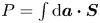 $P = \int \textrm {d}\boldsymbol {a}\boldsymbol {\cdot } \boldsymbol {S}$, where
 $\boldsymbol {S}$ is the time-averaged Poynting flux and
 $\boldsymbol {a}$ is the cross-sectional area of interest. Consider the incident power through the cross-sectional area of dimensions
 $L_z$ and
 $L_y$ on the
 $yz$-plane,
 \begin{equation} P_{\textrm{inc},x} = S_{\textrm{inc},x}L_y L_z. \end{equation}
The equation above is straight-forward because  $S_{\textrm {inc},x}$ is assumed constant. The scattered power radiating away from cylinder is
 \begin{equation} P_{\textrm{sct},\rho}(\rho) = \rho L_z \int_{-{\rm \pi}}^{+{\rm \pi}} S_{\textrm{sct},\rho}(\rho,\theta)\,\textrm{d}\theta. \end{equation}
Only the far-field radiation is considered (and therefore multi-pole effects near the cylinder are neglected). In this case,
 \begin{equation} P_{\textrm{sct},\rho}|_{\textrm{far-field}} = \mathop{\lim}\limits_{\rho \rightarrow \infty} \rho L_z \int_{-{\rm \pi}}^{+{\rm \pi}} S_{\textrm{sct},\rho}(\rho,\theta)\,\textrm{d}\theta. \end{equation}
In general, the far-field radial scattered power  $P_{\textrm {sct},\rho }|_{\textrm {far-field}}$ converges to a non-zero value because
 $S_{\textrm {sct},\rho }(\rho,\theta )\propto 1/\rho$ for large
 $\rho$. From now on,
 $P_{sct,\rho }$ is taken to mean
 $P_{\textrm {sct},\rho }|_{\textrm {far-field}}$. Next, define the scattering width,
 $\sigma$ as
 \begin{equation} \sigma \equiv \frac{P_{\textrm{sct}} L_{y}}{P_{\textrm{inc}}} = \frac{\displaystyle\mathop{\textrm{lim}}\limits_{\rho \rightarrow \infty} \rho \displaystyle \int_{-{\rm \pi}}^{+{\rm \pi}} S_{\textrm{sct},\rho}(\rho,\theta)\,\textrm{d}\theta }{S_{\textrm{inc},x}}, \end{equation}
which has the physical meaning of power scattered per cylinder per incident power/ $L_{y}$ (Myra & D'Ippolito Reference Myra and D'Ippolito2010). Clearly, as
 $L_y$ (the incident beam width in the
 $y$-direction) increases, less power is directly incident on the cylinder. So as
 $L_{y} \rightarrow \infty$, also
 ${P_{\textrm {sct}}}/{P_{\textrm {inc}}} \rightarrow 0$. In reality, the LH beam has a finite width and there are multiple cylinders (SOL filaments) in its path. This allows the cancellation of the
 $L_{y}$ variable. Suppose a beam of width
 $L_y$ is travelling through a turbulent layer of width
 $L_x$. Within that layer are filaments of average radius
 $a_b$. Assuming the cross-sectional packing fraction
 $f_{p}$ of filaments in this layer is known, the beam encounters
 ${f_{p} L_x L_y}/{{\rm \pi} a_b^{2}}$ filaments on average. This can be used to roughly estimate the fraction of incident power scattered from multiple filaments:
 \begin{equation} \frac{P_{\textrm{sct}}}{P_{\textrm{inc}}} \approx \frac{f_{p} L_x}{{\rm \pi} a_b^{2}} \sigma. \end{equation}
This is only valid for a sparse filament layer, because the effects of an already scattered wave interacting with another filament are ignored. This is properly accounted for in the RTE introduced in § 5.