I. INTRODUCTION
As power electronic research has rapidly developed, commercial use of non-linear loads, harmonic contamination, and unbalanced reactive power, which are critical in power systems, have also progressed [Reference El-Habrouk, Darwish and Mehta1–Reference Lascu, Asiminoaei, Boldea and Blaabjerg3]. Researchers aim to improve quality electric energy and have developed current control techniques for active power filters (APF); nevertheless, optimization of such systems remains in demand [Reference Akagi, Nabae and Atoh2–Reference Akagi6]. APF is generally used to improve power quality and overcome limitations caused by natural phenomena, such as switching, connection of high-power non-linear loads, and voltage sags [Reference Rahman and Ratrout7–Reference Daniyal, Borle, Lam and Iu9].
This paper presents a novel design to dynamically adjust ramp-time bandwidth by implementing ramp-time current control with the use of fuzzy logic control (FLC). Selecting the loop width R to represent an APF device for overall current tracking efficiency requires a critical study. Generally, the large loop width R reduces switching frequency but generates high harmonics, whereas the small loop width R increases switching frequency, causes switching losses, and produces high tracking accuracy [Reference Han10, Reference Han11]. In a normal ramp-time method, the characteristics of near-fixed bandwidth can instantaneously modify device switching frequency, resulting in several complications [Reference Han11].
A large difference between sample current and command signal compromises the safety of a device in operating under high frequency, whereas minimal difference may decrease the accuracy of current tracking [Reference Han11]. Several control approaches have been proposed to dynamically modify the loop width R. An APF model integrated with ramp-time current control principles is initially presented and used to analyze variations in switching frequency. An FLC strategy is then implemented to obtain dynamic ramp-time loop. The automatic self-tuning parameter of the ramp-time comparator is achieved and used to improve the efficiency of the proposed method.
Other proposed control approaches include the following: (1) current control bandwidth based on voltage space vector for harmonic component minimization and output voltage control to reduce errors related to current tracking [Reference Saeedifard, Bakhshai and Joos12]; (2) a new method for modulating the space vector pulse width to control direct current (DC) rail resonant inverters, whose controller differs from hysteresis controllers in terms of a second integrator inserted in the forward loop path [Reference Sanbo, Zong-xinag and Jun-min13]; and (3) a bidirectional reactive and real power control, which almost saturates the switching frequency of power devices by modifying the current control loop width [Reference Kumar and Vasudevan14, Reference Poulsen and Andersen15]. Nevertheless, these approaches could not resolve inconsistencies in receiving voltage and current in wireless power transmission (WPT) systems. As such, distorted current or voltage cannot be dynamically monitored and time-varying outputs cannot compensate harmonic signals; hence, practical field tests have not been conducted to verify the effectiveness of these approaches.
Implementation of proposed techniques in WPT systems can provide high-quality output power because of variable distance between transmitter and receiver coils. The use of APF can overcome disturbances that distort the output during transmission. As APF stabilizes output current, power switches rapidly changes switching frequency and may generate problems when they overheat. As such, fuzzy control is important because it creates delay from fuzzy inference to avoid rapid switching, thereby slowing down switching and preventing significant increase and decrease of the output power level in the WPT system.
Application of the proposed method does not only resolve inconsistencies in rapid switching frequency, which are caused by permanent ramp-time bandwidth, but also protects power switch lifespan to ensure stable and safe operation of APF. In this regard, a prototype model has been constructed in this study.
II. STRUCTURE AND BASIC PRINCIPLE
A) Structure of APF
The term APF is generic and applied to power electronic circuits consolidated with power switching devices and passive energy cache circuit materials. The design of this circuitry can be changed depending on the applications to be implemented. This type of circuitry is generally used to regulate current harmonics in a network, supply low- to medium-level voltage distribution, and apply to reactive power with voltage control at a high-voltage distribution level [Reference Peng4–Reference Daniyal, Borle, Lam and Iu9]. A common APF consists of three major elements: inverter, load, and grid.
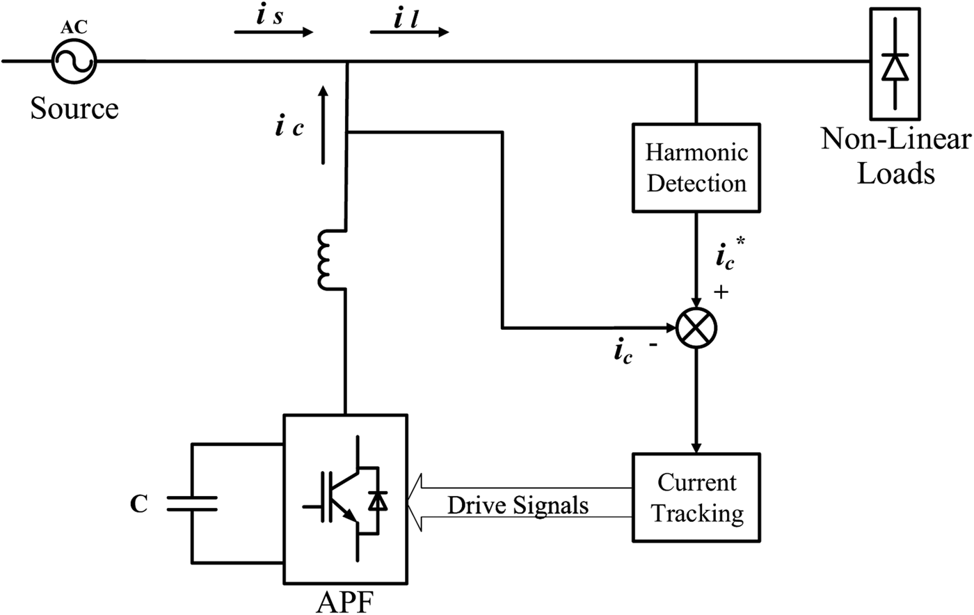
Figure 1 presents a common APF structure linked to a WPT receiving coil; this structure is similar to a power grid connection at a common coupling node over an inductor, which compensates reactive power and harmonics caused by non-linear loads [Reference Akagi6–Reference Qasim, Kanjiya and Khadkikar17].
APF structure.

In the experiment, the APF principle is applied to a single-phase uncontrolled diode bridge rectifier by applying switched-mode power converter, which consists of resistive load to produce harmonic current elimination [Reference Borle18]. The converted power is controlled to generate equal compensation current, which differs from reactive and harmonic currents produced from non-linear loads. Insulated gate bipolar transistor (IGBT) switches is used as voltage source (V s ) of the inverter (one of the major elements in APF), whereas shunt AFP is employed as the energy stored in the DB bus capacitor. Other APF types, such as series and hybrid APF, can also be used.
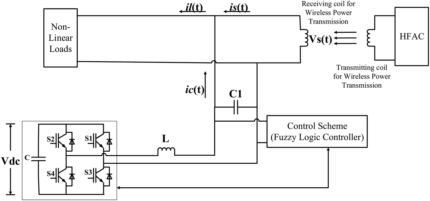
The structure of a single-phase APF is shown in Fig. 2 and analyzed based on variations in switching frequency. V dc refers to the DC voltage capacitor, and V s represents the voltage source. The WPT system is connected to the single-phase APF and controlled by FLC. The distance of the WPT coil can be adjusted according to the requirements.
Structure of single-phase APF.

B) Ramp-time current control principle
Ramp-time current control utilizes near-fixed switching frequency and is set to target 16.67 kHz switching. This setup was originally designed to obtain dynamic performance in terms of hysteresis by maintaining fixed switching frequency. A new version of ramp-time current control, called polarized ramp-time current control, is used in this experiment [Reference Borle18]. This approach can induce current in the converter to follow a specific desired value or the reference current [Reference Saeedifard, Bakhshai and Joos12, Reference Kumar and Vasudevan14, Reference Cirrincione, Pucci, Vitale and Miraoui19–Reference Diaz and Sligo21].
 $${T_{ar2}} = \; \displaystyle{{{T_{ar1}}} \over {{T_{ar2}}}}\; \times \; \displaystyle{{{T_{sw}}} \over 2}.$$
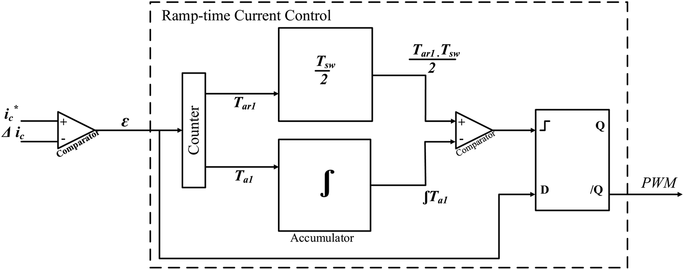
Ramp-time collects information of ε and the output of switching signal (pulse width modulation, PWM) to achieve the value for subsequent switching exponent. Ramp-time current control for WPT systems presents two advantages. The first advantage is the zero average current error (ZACE) status, in which the area of each excursion (β in Fig. 3) is similar to that in previous excursion (α in Fig. 3); this status can be achieved by setting the excursion time T a2 to be equal to the excursion time T b1. Second, ramp-time current control can achieve fixed switching frequency by inducing each excursion time T a2 and T b2 to be equal to the half of switching duration, that is (T sw / 2) as shown in equation (1), to provide stable output current.
Timing of ramp-time current control.

Similar to the other half cycle, T b2 is calculated by using similar equation but T ar2 is replaced with T bf2, T ar1 with T bf1, and T a1 with T b1. Each switching cycle undergoes the same process, thereby confirming that ramp-time can change the value of the next “ramp away time” to produce the next “excursion time” that is similar to the half-switching duration. Therefore, ramp-time current control can be switched at a fixed frequency and nullified the average current error.
The optimal current control can accurately follow the reference current with ZACE in each switching period. Ramp-time current control was applied to determine the ZACE approach with fixed switching frequency [Reference Lisauskas and Rinkevičienė22, Reference Gupta, Boudreaux, Nelms and Hung23]. This approach uses stand-alone current error signals to obtain switching instants and maintain a narrow switching frequency band. In ramp-time current control, every switching/finding is programmed from the latest zero crossing of current error signals. Every switching instant is selected at the appropriate time after the last zero crossing to present excursion from the last zero for the precise part of the desired switching period.
C) WPT system
The experimental setup consists of two self-resonant coils: a transmitter coil that is inductively coupled to an oscillating circuit and a receiver coil that is inductively coupled to a resistive load. Self-resonant coils can achieve resonance depending on the interplay between the distributed capacitance and inductance [Reference Kurs, Karalis, Moffatt, Joannopoulos, Fisher and Soljačić24]. The coils are composed of electrically conductive wire with total length l and cross-sectional radius, which encircles around the cylinder with n turns, height h, and radius r.
An inverter provides constant current to compensate variations in load resistance. A small misalignment between the power transmitter and receiver coils causes variations in the load, resulting in reduced power. As such, the inverter must provide steady magnetic flux through constant current control. In contrast to the inverter controller, the regulator may change the current of the collector to adjust the output power. High pick-up current allows high output power [Reference Kurs, Karalis, Moffatt, Joannopoulos, Fisher and Soljačić24] and causes power losses, such as core loss, winding copper loss, and parasitic resistance loss. Therefore, a system must be controlled to overcome these limitations.
III. CONTROL ALGORITHM
FLC, an artificial intelligence approach, is the control algorithm used in this paper. FLC is well-known because of its transparent system, which can solve simple and complex problems that do not need high accuracy. Most researchers used FLC to deal with non-linearity and uncertainties. The term “fuzzy” refers to the logic involved in dealing with concepts that cannot be indicated as “true” or “false,” rather as “partly true” or “partly false.” Although alternative control approaches, such as genetic algorithms and neural networks, which exhibit similar performance to FLC in most cases, FLC can be modeled in such a way that it can be understood by human operators and, in turn, their practice can be used to design the controller. Hence, mechanical tasks can be easily performed by humans. In this case, FLC is used to control the mutative threshold bandwidth of ramp-time current control and overcome high fluctuations in switching frequency in normal ramp-time current control. Implementation of FLC dynamically alters the constructed ramp-time comparator bandwidth. Compared with other classical controllers, FLC present several advantages, such as simple control, low cost, and feasibility to be designed without knowing the precise mathematical model of the process or system [Reference Rahman and Ratrout7]. FLC systems have been successfully employed to universal approximate mathematical models of a dynamic system. Such systems provide an efficient alternative to classical methods of modeling and control of a nonlinear system (Fig. 4).
Ramp-time current control block.

Prior to FLC implementation to the ramp-time current control in APF, a model is developed in system identification (SI) to verify WPT modeling. SI is used to build mathematical models of a dynamic system by using a set of measured stimulus and response data. This tool is essential for communication and control engineering, as well as in many other areas. The LabView software incorporates SI as an interactive tool to identify the transfer function of the system. This toolkit encompasses the entire identification process from raw data analysis to validation of identified models. In this work, input (reference current and measured current/sense actual current) and output (current value) data were obtained from the prototype model to investigate the SI of the current control model in the LabView software.
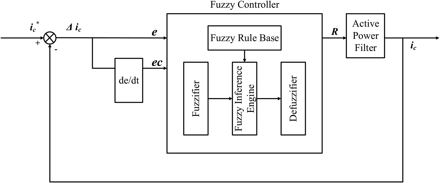
Figure 5 shows the FLC connection diagram, which represents the model of the proposed system connected to APF, with the measured current as the feedback. Fuzzy input is divided into two parts: |Δi c |, which is the reference current and the measured current deviation; and |dΔi c / dt|, which is the change rate of the reference current and the measured current deviation (Fig. 5) before given as input in the FLC block. After derivation, five types of cases are identified:
-
(1) At high values of |Δi c |, the current value is proximal to the zero-crossing point and is correlated with high switching frequency; hence, the loop range R should be immediately increase accordingly;
-
(2) At low values of |Δi c |, the current value is proximal to the peak-value point and is correlated with low switching frequency; hence, the loop range R should be immediately decrease accordingly;
-
(3) At medium values of When |Δi c |, the loop range R is proximal to the value of |dΔi c / dt| regulated by:
-
(a) At high values of |dΔi c / dt|, the proximal current value immediately changes and the loop range R should be increased accordingly;
-
(b) At low values of |dΔi c / dt|, the proximal current value stagnantly changes and the loop range R should be decreased accordingly;
-
(c) At medium values of |dΔi c / dt|, the loop range R remains constant.
-
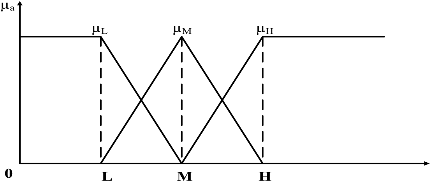
Therefore, the fuzzy relationship consists of two inputs, namely, ec and e, which act as |dΔi c / dt| and |Δi c |, respectively, and the output is the loop width R. Antecedent and consequence can be determined by identifying and examining cases that may occur because of the APF system behavior. During fuzzication, the input is classified into three classes: low (L), medium (M), and high (H). The Mamdani method is used to obtain crisp output [Reference Brown and Harris25]. Figure 6 represents the membership function of the input, which comprises the same shape for both input (|Δi c | and |dΔi c / dt|) and output, (R). Crisp output refers to an output that provides result to the nearest value to prevent rapid changes in switching frequency.
Schematic diagram of FLC.

Membership function for |Δi c | and |dΔi c / dt|.

Crisp output is represented by R = [R 1, R 2, R 3, R 4, R 5], and each value from R 1 to R 5 varies in different cases. The membership function during fuzzication is evaluated according to the APF inference. The fuzzy rules, which consider each weight of membership, are shown below:
Rule 1:
 $$\eqalign{& {\rm If}\, \left\vert {\Delta {i_c}} \right\vert = {\rm High},\quad {\rm then}\;R = {R_1},\; \cr & \;\;{\mu _1}\left( {\left\vert {\Delta {i_c}} \right\vert,\left\vert {\displaystyle{{d\Delta {i_c}} \over {dt}}} \right\vert} \right) = {\mu _{aL}}(\left\vert {\Delta {i_c}} \right\vert);}$$
Rule 2:
 $$\eqalign{{\rm If}\, \left\vert {\Delta {i_c}} \right\vert & = {\rm Medium},\quad {\rm and}\;\;\left\vert {\displaystyle{{d\Delta {i_c}} \over {dt}}} \right\vert = {\rm High}, \cr & \quad \,\,{\rm then}\;R = {R_2},\;\;\;{\mu _2}\left( {\left\vert {\Delta {i_c}} \right\vert,\left\vert {\displaystyle{{d\Delta {i_c}} \over {dt}}} \right\vert} \right) \cr & = {\mu _{aM}}(\left\vert {\Delta {i_c}} \right\vert){ \cap ^{{\mu _{bL}}}}\left( {\left\vert {\displaystyle{{d\Delta {i_c}} \over {dt}}} \right\vert} \right);} $$
Rule 3:
 $$\eqalign{{\rm If}\, \left\vert\Delta {i_c}\right\vert & = {\rm Medium},\quad {\rm and} \left\vert {\displaystyle{{d\Delta {i_c}} \over {dt}}} \right\vert = {\rm Medium}, \cr & \quad \,\,{\rm then} \, R = {R_3},\quad {\mu _3}\left( {\left\vert\Delta {i_c}\right\vert,\left\vert {\displaystyle{{d\Delta {i_c}} \over {dt}}} \right\vert} \right) \cr & = {\mu _{aM}}(\left\vert\Delta {i_c}\right\vert){ \cap ^{\kern 1pt} }{\mu _{bM}}\left( {\left\vert {\displaystyle{{d\Delta {i_c}} \over {dt}}} \right\vert} \right);} $$
Rule 4:
 $$\eqalign{ {\rm If}\,\left\vert\Delta {i_c}\right\vert & = {\rm Medium},\quad {\rm and}\left\vert {\displaystyle{{d\Delta {i_c}} \over {dt}}} \right\vert = {\rm Small}, \cr & \quad \,\,{\rm then}\;R = {R_4},\quad {\mu _4}\left( {\left\vert\Delta {i_c}\right\vert,\left\vert {\displaystyle{{d\Delta {i_c}} \over {dt}}} \right\vert} \right) \cr & = {\mu _{aM}}(\left\vert\Delta {i_c}\right\vert){ \cap ^{{\mu _{bS}}}}\left( {\left\vert {\displaystyle{{d\Delta {i_c}} \over {dt}}} \right\vert} \right);} $$
Rule 5:
 $$\eqalign{{\rm If} \vert \Delta {i_c} \vert &= {\rm Small},\quad {\rm then}\; R = {R_5},\quad {\mu _{5{\rm \;}}} \left( { \vert \Delta {i_c} \vert, \left \vert {\displaystyle{{d\Delta {i_c}} \over {dt}}} \right \vert} \right) \cr& = {\mu _{aS}}( \vert \Delta {i_c} \vert ).} $$
Understanding engineering concepts plays an important role in deciding the value of the loop width R i , which decreases from R 1 to R 5 (R 1 > R 2 > R 3 > R 4 > R 5) when both switching frequency and current tracking precision are investigated. In Rule 3, both |dΔi c / dt| and |Δi c | are near-medium linguistic variables and the general medium loop width value is advisable, which is mainly fixed by inherent switching frequency range of the power device. In Rule 5, the minimum loop width value should be selected to obtain high precision and small tracking error. In this work, the values of R 1 to R 5 are set to 16, 14, 10, 8, 6, and 4 for each loop width.
Each loop width from R 1 to R 5 yields different control reactions. Assuming that physical switching frequency reaches the maximum permitted in a power switch, a small bandwidth and high-precision current tracking are obtained. However, if switching frequency reacts fast that it almost achieves the zero-current crossing point, the FLC will not rapidly trigger the loop width within a short period of time because of delay in fuzzy inference. This phenomenon ensures that the safety allowance designed to conserve power switches up to the limit permitted in switching frequency is examined. Rapid changes in switching frequency before FLC implementation are due to the inconsistent air gap range of the WPT coil.
A prototype of WPT coil connected to an APF prototype with FLC in ramp-time current control was developed to verify the hypothesis. The WPT coil was placed on 0 cm for the first reading, and the range was increased to the maximum of 20 cm air gap between the transmitter and receiver. The power rate was recorded at 128–35 W.
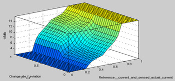
Figure 7 shows the surface viewer of FLC, which is commonly known as control surface. Surface viewer is a convenient tool used to examine or identify a control strategy with two inputs and one output. Surface viewer is a three-dimensional (3D) curve that represents the entire mapping from the reference current and measured current deviation to the change rates of these parameters. However, beyond 3D, difficulties in displaying the results are encountered. In this 3D graph, inputs are represented from the base of the graph, whereas outputs are represented by the height of the graph above each input pair. Loop width in any discrete time for the overall ramp-time current control with FLC is calculated using equation (2), where the value of loop width R must be set to the desired value, PWM switching signal, and comparator device threshold.
 $$R = \displaystyle{{\mathop \sum \nolimits_{i = 1}^5 \left[ {{\mu _i}\left( { \vert \Delta {i_c} \vert, \left \vert {\displaystyle{{d\Delta {i_c}} \over {dt}}} \right \vert} \right){R_i}} \right]} \over {\mathop \sum \nolimits_{i = 1}^5 {\mu _i}\left( { \vert \Delta {i_c} \vert, \left \vert {\displaystyle{{d\Delta {i_c}} \over {dt}}} \right \vert} \right)}}.$$
Surface viewer of FLC.

Throughout the process, loop width at any time can be established by setting the value of R to be comparable with the device threshold; hence, PWM switching signals will be generated as shown in equation (2). The final step in FLC is defuzzification using the center of gravity method to obtain the precise value of R [Reference Pedrycz and Gomide26].
IV. SIMULATION ANALYSIS
Prior to implementation of ramp-time current control with FLC, an experimental comparison was performed to compare and determine the performance of different types of approaches, such as proportional-integral (PI) and hysteresis current control, in terms of output current distortion in the APF node. The percentage of accuracy is calculated using equation (3) to compare the generated grid current with the reference current. Hence, the percentage of accuracy may result in bias differences between fixed and non-fixed switching frequency of current control. %Accuracy is associated with all variances from the reference and involves the fundamental component tolerance and the measured DC component error, which is not denoted by harmonic “distortion.” Therefore, in a mathematical form:
 $$\% {\rm Accuracy} = \displaystyle{1 \over {{i_{ref,rms}}}}\sqrt {\displaystyle{1 \over T}\int_T^T {{{\left( {{i_{resultant}} - {i_{ref}}} \right)}^2}dt}} \times 100.$$
THD i in equation (4) refers to the total current harmonic distortion, which is commonly used to imply distortion. However, total demand distortion is another term used to indicate distortion and can be found in IEEE 519 standard [27].
 $${\rm TH}{{\rm D}_i} = \displaystyle{1 \over {{i_{resultant,i}}}}\sqrt {\mathop \sum \limits_{n = 2}^\infty i_{resultant,n}^2} \times 100.$$
Lower order current harmonics distortion (LHD i ) in equation (5) is obtained from THD i but does not include harmonic order higher than 21. Hence, low-frequency distortion was obtained by using fast Fourier transform (FFT) based on the resultant current, resulting in dynamic switching frequency. From this equation without the switching attempt, the results are predicted to be almost zero if the resultant current, including the reference, is in sinusoidal form and phase. Therefore, LHD i is expressed as equation (5).
 $${\rm LH}{{\rm D}_i} = \displaystyle{1 \over {{i_{resultant,i}}}}\sqrt {\mathop \sum \limits_{n = 2}^{21} i_{resultant,n}^2} \times 100.$$
Table 1 shows %Accuracy, LHD i , and THD i for the source current i s and the grid current i grid . Although hysteresis current control is the fastest and provides higher %Accuracy compared with Ramp-time in i s , it does not provide the lowest distortion on i grid because of dull time, variable switching frequency, and low-order harmonics [Reference Buso, Malesani and Mattavelli28]. As evidenced by the highest reading from Table 1, ramp-time current control is among the approaches with the highest %Accuracy. As such, ramp-time control has been selected for the experiment because of its near-fixed switching frequency characteristics, which are wider than PI current control.
Performance of each types of current control.

The WPT behavior was completely simulated in the LabView software by using parameters, namely, receiving voltage versus distance between the transmitter and receiver coils. The distances are 0, 4, 8, 12, 16, and 20 cm, and the corresponding receiving voltages are 38, 34, 30, 22, and 16 V, which represent the grid source line voltage in APF; R ms value and V s , as shown in Fig. 2, are obtained depending on the dynamic sampling period over time. The line capacitor and inductor used is 4500 µF (DC capacitor) and 1 mH, respectively. The coil is arranged in symmetrical configuration, and the highest switching frequencies used are 5, 10, and 15 kHz.
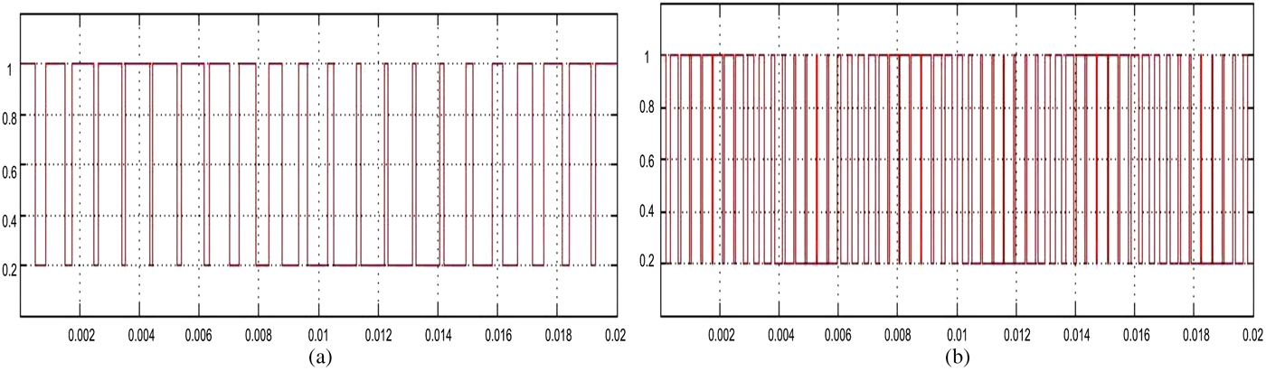
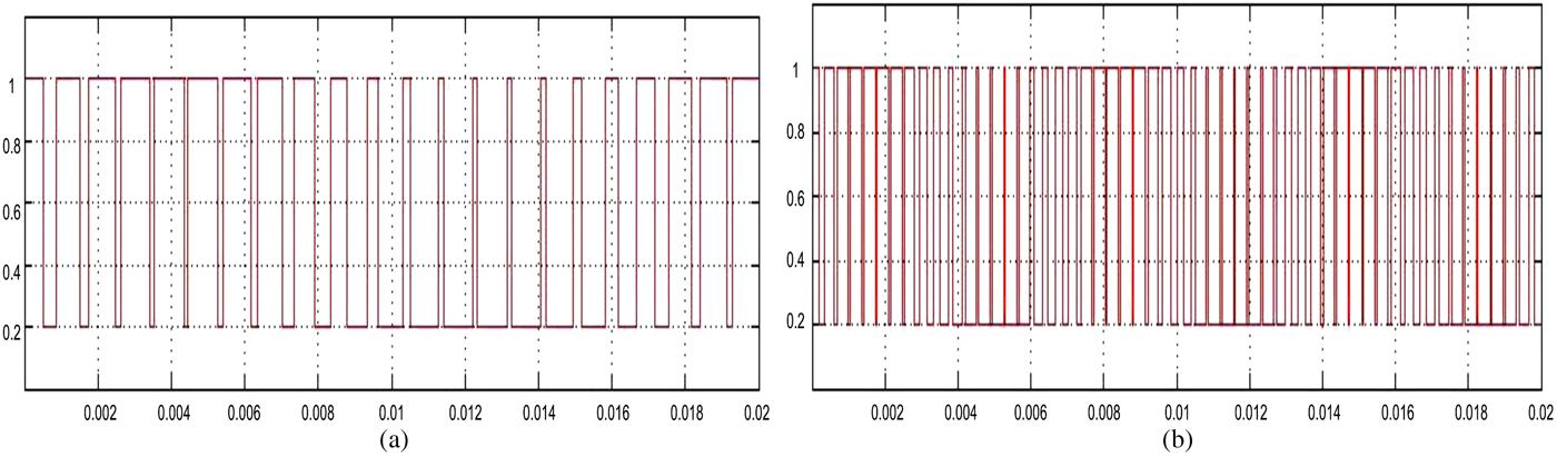
Figure 8 shows the switching signal for the PWM pulses of single-phase simulation waveforms. The figure shows the effectiveness of ramp-time current control with FLC toward the output and confirms that the gap between each pulse is closer and produces smooth switching signal for PWM.
Simulation waveform of PWM (a) before and (b) after new approach implementation.
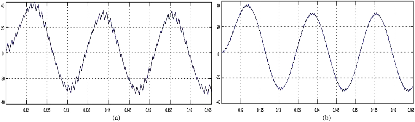
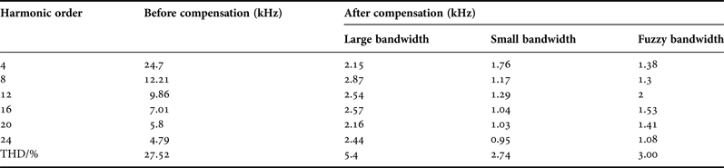
Further investigation of the two steady-state cases is shown in Table 2. When using ramp-time with large bandwidth, the switching frequency is low but the current waveform is insufficient because it presents glitches and cannot provide a compensating effect. However, in the approach with small bandwidth, the output current and switching frequency are higher than the highest switching frequency allowed, thereby causing adverse effects on APF devices. Compared with the ramp-time method, the ramp-time control method incorporated with fuzzy threshold exhibits a perfectly smooth output current waveform, as shown in Fig. 9(b).
Spectrum analysis of current waveform: (a) ramp-time current control (b) ramp-time current control with FLC.
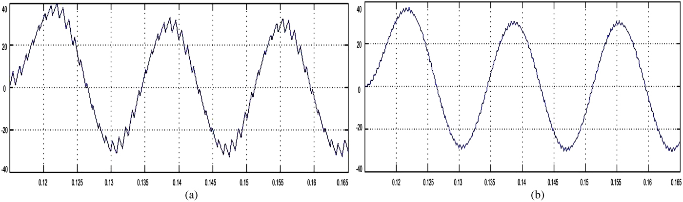
Current frequency in steady-state comparison.

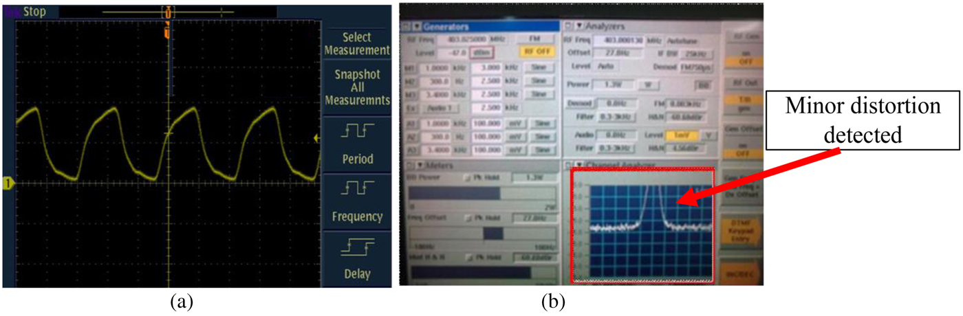
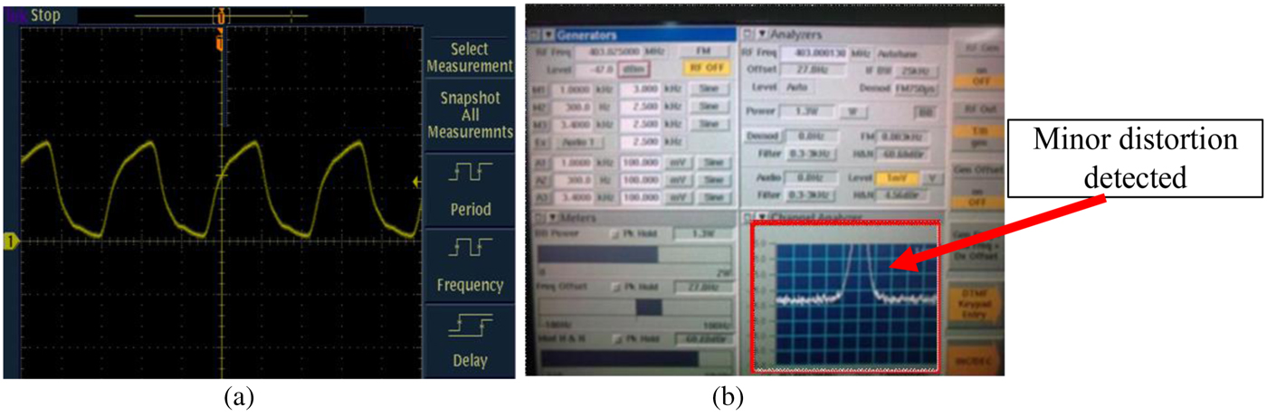
Figure 10 shows the waveforms of the output current for a standalone ramp-time current control. Based on the signal measured from normal oscilloscope, only minor distortions are detected, which rapidly changes the switching frequency. However, with the use of spectrum analyzer, as shown in Figure 10(b), a critical distortion rated at 1.1 V occurs and can be eliminated using delay of FLC inference.
Current waveform spectrum analysis with ramp-time current control strategy and without FLC: (a) from oscilloscope and (b) from spectrum analyzer.
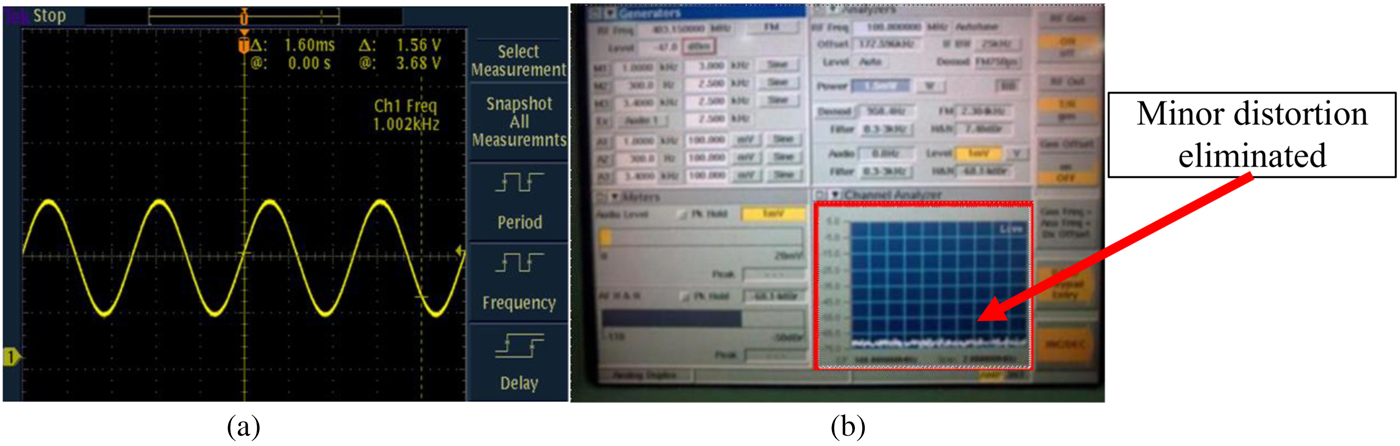
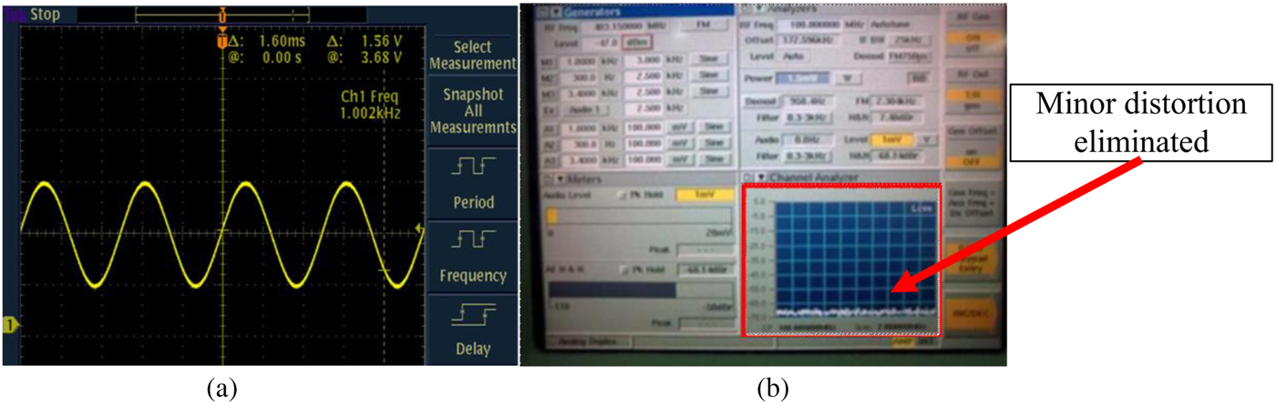
As shown in Fig. 11(a), normal oscilloscope did not detect any distortion and shows an almost perfect sine wave, thereby confirming that FLC changed the results. Meanwhile, discrete distortion can be detected by using the spectrum analyzer at 1 mV rate; such distortion occurred because of the tolerance of power switches and other electronic devices used in the experiment. Only minor distortion can be measured using a spectrum analyzer in Fig. 11(b), and critical distortion detected earlier was eliminated. The elimination of minimal distortion could be mainly attributed to the characteristic of the resonant WPT, which reacts sensitively to small changes in the distance between coils. Other elements that contribute to this distortion include the surrounding electrostatic charges and the disturbance from communication devices because the experiment was not performed in a frequency-shielding chamber (anechoic).
Current waveform spectrum analysis with ramp-time current control strategy and FLC: (a) from oscilloscope and (b) signal from spectrum analyzer.
V. CONCLUSION
This paper presents a novel ramp-time current control strategy equipped with FLC to dynamically modify the loop width of the system. The proposed strategy exhibits three advantages:
-
(1) The smoothness of current waveforms caused by thorough current tracking is enhanced by appropriately decreasing the bandwidth.
-
(2) Switching frequency can be prevented to reach the maximum limit of power switches. As such, the damage percentage caused by over-limit switching frequency decreases compared with that in standalone ramp-time current control approach.
-
(3) The approach enables stable output current for WPT even if the distance between coils varies.
The efficiency of the proposed approach will be tested in an industrial site for production usage. This paper is presented based on the industrial FPGA-based hardware and LabView software implementation of APF. Additional implementation proposed for this filter not only fulfills the requirements of dynamic characteristics and rigorous control but also achieves high capacity. Hence, an experiment must be performed to examine the simulation performance of APF under a regular case.
ACKNOWLEDGEMENTS
The authors would like to thank Dr. O.H. Narayan from Motorola Solutions (M) for the support throughout this project. This work was supported in part by University of Malaya Research Grant (UMRG) Project RP006E-131CT and in part by Motorola Solutions (M) Sdn. Bhd.
 Leong Wen Chek received his degree in Electrical Engineering (Electronics) from the Universiti Malaysia Pahang in 2013 and currently pursuing his Ph.D. degree in Power Electronics and Renewable Energy field in the University of Malaya. His main research interests are design and optimization of wireless power transmission using modulated microwave supported by Motorola Solutions (M) Sdn Bhd.
 Saad Mekhilef received his B. Eng. degree in Electrical Engineering from the University of Setif, Setif, Algeria, in1995, and M. Eng. Sc. and Ph.D. degrees in Electrical Engineering from the University of Malaya, Kuala Lumpur, Malaysia, in1998 and 2003, respectively. He is currently a Professor in the Department of Electrical Engineering, University of Malaya. He has been actively involved in industrial consultancy, for major corporations in the power electronics projects. He is the author and co-author of more than 100 publications in international journals and proceedings. His research interest includes power conversion techniques, control of power converters, renewable energy, and energy efficiency.
 Erwan Sulaiman received his B. Eng. degree in Electrical Engineering from the University of Malaya, Malaysia, in 2001, and M. Eng. Sc from Universiti Tun Hussein Onn, Malaysia and Ph.D. degrees in Electrical Engineering from Nagoya Institute of Technology, Japan, in 2004 and 2012, respectively. He is currently a Senior Lecturer in the Department of Electrical Engineering, Universiti Tun Hussein Onn. His interest of research is power electronics, drives, and motors.
Macwien Krishnamurthi received his degree in the engineering council examination from United Kingdom in Electrical and Electronics Engineering in 1993. He is now currently working in Motorola Solutions (M) Sdn Bhd as Distinguished Member of Technical Staff (Electrical and Electronics) in Research and Development, (R&D) Department since 1994. His achievement includes nine patents granted/issued, three patents pending, and two Engineering Awards. He is also Chartered Engineer with the Institution of Engineering and Technology, UK. (C Eng, IET). His research interest; vehicular charger, FM, MSHA Ni, XTS Hicap batteries, and AC–DC and DC–DC power supplies.