Improving the Scree Plot for the Number-of-Factors Decision

Dimensionality-reduction techniques such as Exploratory Factor Analysis (EFA) and Principal Component Analysis (PCA) usually require researchers to determine the number of components or factors to retain (Costello & Osborne, Reference Costello and Osborne2005). One of the most widely used methods for this purpose is Cattell’s scree test (Cattell, Reference Cattell1966; Horn & Engstrom, Reference Horn and Engstrom1979).

The scree test is a heuristic graphic method that consists of: a) plotting the eigenvalues (y-axis) against the components (x-axis), and b) inspecting the shape of the resulting curve in order to detect the point at which the curve changes drastically (and the “scree on the hill slope” begins). This point on the curve indicates the maximum number of components to retain. While the approach is simple and generally useful, such an intuitive but also fuzzy procedure has been criticized as subjective (Zwick & Velicer, Reference Zwick and Velicer1982).

The present paper describes how a data visualization approach based on interactive and dynamic graphics can enhance the scree plot’s capabilities and therefore facilitate decisions regarding the number of factors to retain. The improvements we propose fall into two categories: internal and external. Internal improvements include enhancements that make the scree plot more informative and easier to read, thus improving its validity; for example, displaying the results of a Parallel Analysis on the scree plot itself (Beauducel, Reference Beauducel2001; Horn, Reference Horn1965). External improvements are those designed to complement the scree plot with information from other graphics; for example, linking the scree plot with another statistical graphic or presenting it simultaneously with other plots in the same structured visualization. These improvements offer a more comprehensive interpretation of the scree plot and promote better decision-making by considering other important aspects in the factor analysis result (e.g., factor loadings).

This paper is organized as follows: first, we introduce an example using real data on which a PCA analysis is appropriate, and describe the Cattell’s scree test applied to this data, highlighting the potential weaknesses of this application; second, we describe the two types of proposed improvements; and, lastly, we discuss the proposals and present our conclusions.

Example: Driving Style Data Set

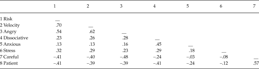
To illustrate the proposed improvements, we will use a data set with eight driving style measures (variables) from a sample of 399 Argentine drivers (participants). The variables represent the different sub-scales of the MDSI (Multidimensional Driving Style Inventory, Taubman-Ben-Ari, Mikulincer, & Gillath, Reference Taubman-Ben-Ari, Mikulincer and Gillath2004), a set of measures related to adaptive and maladaptive driving behaviors on the road. Table 1 shows the Pearson correlation matrix for these sub-scales. In this case, we used factor analysis to explore the structure of the relationships between variables and to determine whether these relationships can be explained by a smaller number of latent dimensions.

Table 1.

Correlation matrix of eight driving-style measures for a sample of Argentine drivers

Note: (1) Risk-taking style, (2) High-velocity style, (3) Angry and aggressive driving style, (4) Dissociative and inattention driving style, (5) Anxious driving style, (6) Stress reduction style, (7) Careful driving style, and (8) Patient driving style.

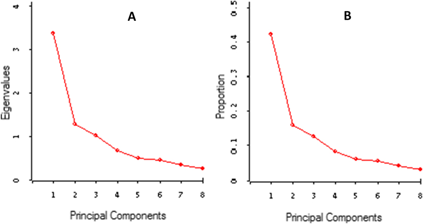
By analyzing Table 1, we obtained a scree plot similar to the one presented in Figure 1. Both of the graphs in Figure 1, “A” and “B,” are essentially the same, except that “A” shows the absolute eigenvalues of the components, while “B” represents the relative proportion of variance accounted for by the components. The scree plot shows that the eigenvalue of the first component is larger than that of the second, and that the second is larger than that of the third, and so on. The important issue here is to evaluate if the variance accounted for by a few of the first eigenvalues can be regarded as sufficient so that we can focus on them and ignore the rest of the components as noise.

Figure 1:

Scree plot representing the eigenvalues (A) and the proportion of variance accounted for by the principal components (B). PCA on the correlation matrix in Table 1.

Cattell (Reference Cattell1966) suggested looking for the point at which the last significant drop or break takes place—in other words, where the line levels off. The logic behind this method is that this point divides the important or “major” factors from the minor or “trivial” factors. Unfortunately, this definition of where the drop occurs is rather vague. Thus, in Figure 1, some may say that this drop occurs after the first component and that, consequently, a single factor should be retained. However, a second drop with a less pronounced slope occurs after the third factor. Hence, the purely visual inspection of the scree plot alone does not produce a clear and unambiguous interpretation. In fact, we solicited the opinion of six experienced researchers in our vicinity as to the number of dimensions to consider based on the plot in Figure 1. The results were surprising. The six researchers gave varying responses, ranging from one to four factors. They all agreed that, in this case, more information is needed on the factor solution to make a decision as to the number of factors to retain. It was also surprising that none of the researchers mentioned the need to use an alternative rule (e.g., Parallel Analysis). This experiment illustrates some of the scree plot's limitations, and also suggests that researchers usually take into account other aspects of the factor solution to determine the number of factors to retain. These complementary interpretation criteria include: the factor loadings of variables; the percentage of variance accounted for by the components; and the interpretability of the resulting factors.

Others have previously pointed out the lack of an objective definition for the cutoff point that separates the important factors from the trivial factors in the scree plot (Zwick, & Velicer, Reference Zwick and Velicer1986). For example, Hayton, Allen, and Scarpello (Reference Hayton, Allen and Scarpello2004) remark that: “Although the scree test may work well with strong factors, it suffers from subjectivity and ambiguity, especially when there are either no clear breaks or two or more apparent breaks” (p.193). Indeed, whereas some studies have reported satisfactory inter-rater reliabilities with several examiners (e.g., Cattell & Vogelmann, Reference Cattell and Vogelman1977; Zwick & Velicer, Reference Zwick and Velicer1982), others indicate that scree plot interpretations often lack consistency and depend heavily on the training received by the examiners and on the nature of the solution (Zwick & Velicer, Reference Zwick and Velicer1986). These authors also suggest that the scree test has a general tendency to overestimate the number of factors to retain.

In summary, the scree test provides an interesting first step in the process of analyzing the dimensionality of a data set, but it is limited as a means of determining the number of factors to retain because it is open to subjective interpretation. Hence, researchers usually have to consider both substantive and statistical issues when deciding on the number of factors to retain (Fabrigar, Wegener, MacCallum, & Strahan, Reference Fabrigar, Wegener, MacCallum and Strahan1999). We maintain that the standard application of the scree plot may benefit from the additional information provided by the complementary methods proposed in this paper. Specifically, we believe that modern dynamic and interactive data visualization techniques (Young, Valero-Mora, & Friendly, Reference Young, Valero-Mora and Friendly2006) provide us with the means to design and implement such enhancements. Although the most widely used statistics packages do not always include such dynamic applications, other powerful resources like ViSta “The Visual Statistics System” (Molina, Ledesma, Valero-Mora & Young, Reference Molina, Ledesma, Valero-Mora and Young2005; Young, Reference Young1996) are available and provide tools to facilitate thorough implementations like the ones we propose here for the scree plot. The remainder of this paper will describe a number of improvements to the scree plot based on the use of dynamic graphics developed with the ViSta software.

Improving the Scree Plot

The suggested improvements fall into two categories: i) internal improvements, such as adding interactive and dynamic features, as well as results from Parallel Analysis (PA) (Horn, Reference Horn1965), to the standard scree plot display; and ii) external improvements, such as linking the scree plot to other displays of interest to help interpret results. Each improvement category will be discussed below in separate sections.

Adding Parallel Analysis Results to the Scree Plot

Due to the usefulness of PA, we propose an enhanced scree plot that combines the results of both methods in a single graph and uses dynamic graphics to enable the user to explore the combined graph more easily. Additionally, we will display some basic improvements that are simpler and computationally less demanding than PA.

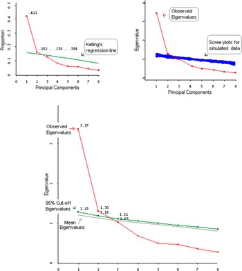
Figure 2 shows three plots that have PA information included in the scree plot for the driving style data example. The top left plot displays the standard scree plot with a Keelling’s regression line (Keeling, Reference Keeling2000). This line approximates the random cut-off eigenvalues given the sample size and number of variables. In our example, only the first two factors would be retained, since the others have eigenvalues below the regression line. However, it is important to note that this regression line estimates the mean of the random eigenvalues in place of the 95th percentile values, which is recommended as a less liberal criterion. Hence, this regression approach may be useful as a way to approximate the PA solution in cases where a Monte Carlo simulation is difficult to run because of the large number of variables and/or observations. In other cases, we can carry out a PA to estimate the 95th percentile values as cut-off criteria for determining significant eigenvalues.

Figure 2:

The PA scree plot. Scree plot plus the parallel analysis results.

The bottom plot adds a line indicating the 95th percentile eigenvalues obtained in a Monte Carlo PA. The eigenvalues observed above this percentile indicate the correct number of components to retain. Again, the PA result on this data suggests retaining the first two factors. The third plot displays the same line as the second plot but computed using the Buja and Eyuboglu (Reference Buja and Eyuboglu1992) multivariate permutation method instead. As PA is relatively robust to deviations from the assumption of multivariate normality, the plot is very similar to the previous one (Buja & Eyuboglu, Reference Buja and Eyuboglu1992).

Adding Dynamic-Labeling Capabilities to the Scree Plot

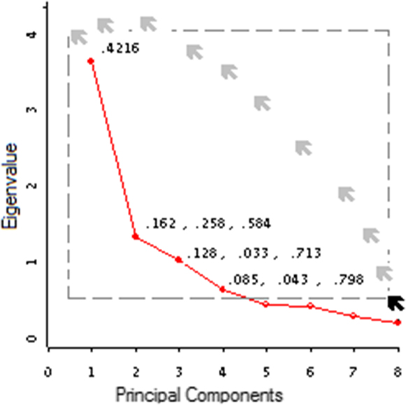
Figures 3 and 4 depict simple improvements to the scree plot. In both cases, new information is added to the plot to facilitate interpretation. This information can also be queried by the user, so specific values of elements can be examined if need be. Figure 3 shows “dynamic labeling” developed in ViSta. In this case, this feature offers important information about the PCA solution (explained variance). By selecting the points with the mouse, a list of values is displayed on the screen: i) the first value is the proportion of data variance accounted for by the component; ii) the second is the difference in explained variance with respect to the previous component; and iii) the third value represents the proportion of cumulative variance. In our example, we observe that the first two factors together explain 58% of the variability (cumulative variance), although the first factor is more important since it accounts for 42% of the total variance. In practice, researchers take these values into account; consequently, adding them to the scree plot can be useful.

Figure 3:

Labeling the scree plot’s points by the proportion of variance accounted for.

Figure 4:

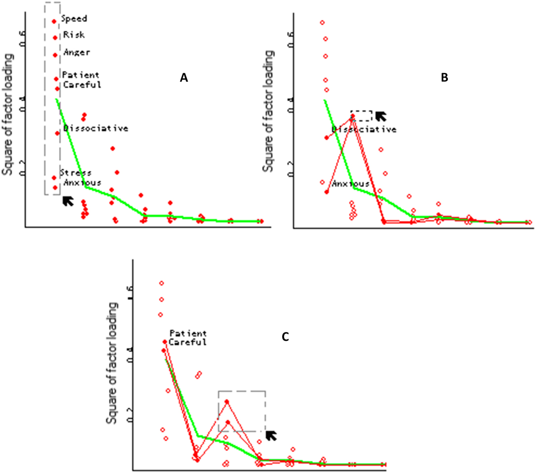
Scree plot and squared factor loadings.

Figure 4 illustrates a more sophisticated form of dynamic labeling. It shows a scree plot that incorporates points representing the squares of the factor loadings for the variables. The squared factor loadings can be interpreted as the percentage of the variable's variance that is explained by a component or factor. The variance explained by a component is the average of the squared factor loadings of the variables in that component. If we represent both the squared factor loadings and its means through all the factors, we obtain a graph like the one shown in Figure 4.

The charts in Figure 4 are essentially scree plots, since the means line coincides with the proportion of variance explained by the factors (eigenvalues). But they add important information on how the variables are explained by each factor. In this case, by directly selecting the plot points, the names of the variables are displayed on the screen.

In plot (a), all variables have been selected in the first factor. We observe that risky, speedy and angry driving styles have the highest values in this factor, followed by the careful and patient styles. In plot (b), the variables with the highest values in the second factor have been selected, which turn out to be the anxious and dissociative driving styles. The last chart shows the selection of the third factor, where careful and patient styles are highlighted. With this enhancement to the scree plot we get a picture of the relative importance of the factors, as well as their theoretical meaning. In this way, the scree plot increases its exploratory power.

External Improvements: Linking the scree plot with other dynamic graphics

Interpreting factor analysis results usually requires the consideration of various sources of information. Thus, it can be very useful in practice to complement the scree plot with information stemming from other sources, especially when that information can be visualized simultaneously. The dynamic-graphics capability called “linking” (Cleveland & McGill, Reference Cleveland and McGill1988; Young et al., Reference Young, Valero-Mora and Friendly2006) is an excellent way to achieve this purpose and to improve the use of the scree test as a tool to determine the number of factors to retain.

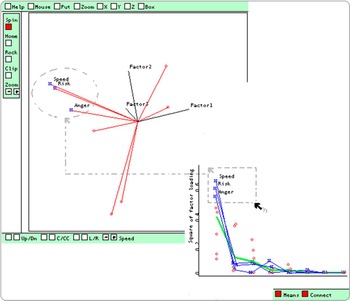
Linking (Becker, Cleveland, & Wilks, Reference Becker, Cleveland and Wilks1987) is a graphical technique that connects corresponding points from two or more scatterplots. For example, given the four variables a, b, c, and d, let graph 1 be the variable b against the variable a, and graph 2 be d against c. Linking is any computational method that visually connects the point (a_k, b_k) from graph 1 to the point (c_k, d_k) from graph 2. Figure 5 displays a scree plot linked to a spin-plot in ViSta (Young et al., Reference Young, Valero-Mora and Friendly2006). The spin-plot presents a three-dimensional graphic that the user can spin to observe the factor loadings in the space of the principal components. It uses vectors to represent the variables on the principal components. In Figure 5, we see that the most salient variables in the first factor (risky, speed and angry) have been selected. As a result, these variables are highlighted in the spin-plot, where we can observe their closeness in the principal components space.

Figure 5:

An image of a scree plot linked with a spin plot.

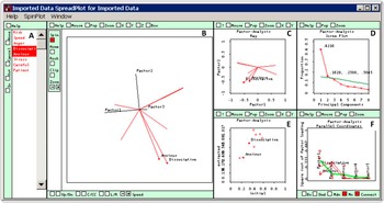
More sophisticated versions of linking are incorporated into the spreadplot, a data visualization technique consisting of multiple dynamic graphics showing several aspects of the same statistical result (Young, Valero, Faldowsky, & Bann, Reference Young, Valero-Mora, Faldowski and Bann2003). The plot-windows comprising a spreadplot work together in a dynamic way, so that changes by the user in one window produce automatic corresponding changes in the rest. Figure 6 depicts a spreadplot designed to explore the results of a principal components analysis that includes a scree plot. This visualization is based on previous research by Ledesma, Molina, Young, & Valero-Mora (Reference Ledesma, Molina, Young and Valero-Mora2007). The spreadplot incorporates: (a) a window listing variable names; (b) a spin-plot with the factor loadings of the variables; (c) a scatterplot with the variable loadings; d) a scree plot with a regression line estimating the cut-off eigenvalues; (e) a scatterplot showing initial versus after-factor-extraction communalities; and f) a scree plot with the squared factor-loadings. This is a very useful graphical strategy to help researchers determine the number of factors to retain. As various authors have indicated, the decision on how many factors to retain cannot be based solely on the application of a given cut-off rule; other relevant statistical and theoretical aspects should be considered, such as the number of variables loading by factor and the meaning and interpretability of the factor solution. Spreadplots allow researchers to simultaneously observe and analyze other relevant information together with the scree plot.

Figure 6:

The scree plot incorporated in a spreadplot visualization for Factor Analysis.

Further Possibilities with Dynamic Graphics

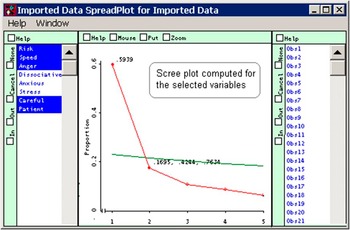
Dynamic graphics can help researchers simplify and improve other aspects of factor analysis. For example, consider the case of psychometric analysis at the item-level. In this context, it is common to carry out successive analyses based on different subsets of items (Velicer, Reference Velicer1976). This is typically performed by including or excluding variables, and re-computing the results of a factor analysis. Figure 7 shows how this process can be simplified using dynamic ViSta graphics. The list of variables on the left of Figure 7 allows us to select and deselect variables. Whenever the state of a variable is changed, the software re-computes the result of the analysis and displays a new scree plot comprised only of the selected variables. In the example, the variables with high loadings on the second factor (i.e., anxious, dissociative and stress) have been excluded from the analysis. As a result, the factor solution becomes one dimensional. Thus, ViSta’s scree plot applications achieve more efficient and thorough performance than other alternative statistics packages that lack linking procedures and multiple dynamic graphics.

Figure 7:

Dynamic computation of the scree plot.