2.1. Derivation of the model

Dual-layer systems exhibit substantially enhanced complexity in wave–interface inter- actions compared with single-layer configurations, with the interplay of the coupled interface dynamics and reverberating waves posing substantial challenges for quantitative analysis (Mikaelian Reference Mikaelian1985). To isolate these effects, our model simplifies the system by maintaining flat geometries for both the light–heavy interface (AI) which is the first shock-impacted interface, and the upstream heavy–light interface (UI). This geometric design choice effectively suppresses perturbation growth at AI while eliminating its interaction with UI, thereby allowing focused analysis on the UI and downstream heavy-light interface (DI). Despite these simplifications, the presence of AI introduces additional wave-reverberation pathways within the dual-layer structure. Consequently, the perturbation evolution at DI remains inherently more complex relative to single-layer systems, as reverberation waves from AI persistently modulate the vorticity distribution at the interface. This controlled reduction of variables provides a foundational framework for resolving dual-layer instability mechanisms while preserving key physical drivers of multi-interface coupling.

Figure 2.

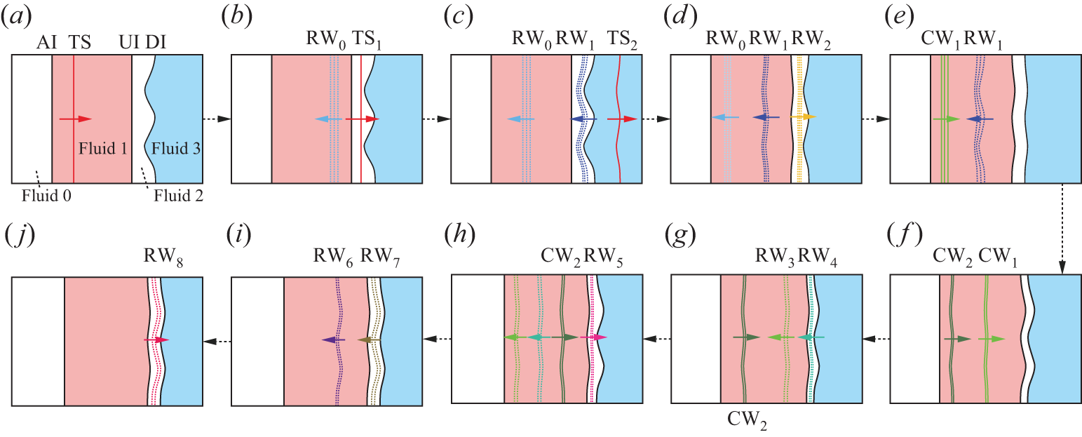
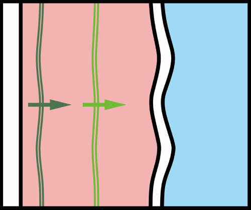
Schematic diagrams of a shock accelerating a fluid dual-layer which contains a AI and two successive heavy-light interfaces. (a) The incident shock has passed through the first AI, generating the transmitted shock (TS), which is about to impact the upstream UI; (b) the rarefaction waves (RW $_0$ ) moving towards AI are generated by TS interacting with UI and the second transmitted shock (TS $_1$ ) moves to DI; (c) after TS $_1$ passes through DI, the third transmitted shock (TS $_2$ ) is generated and the rarefaction waves RW $_1$ moving to UI are reflected; (d) after the RW $_1$ pass through UI, rarefaction waves RW $_2$ are reflected to move to DI and the RW $_1$ move to AI following RW $_0$ ; (e) RW $_0$ has struck AI, the reflected compression waves CW $_1$ are formed, while the RW $_1$ have not reached AI and are about to collide with CW $_1$ ; (f) after the RW $_1$ interact with AI, the compression waves CW $_2$ are generated and move to UI following CW $_1$ ; (g) the CW $_1$ , respectively, accelerate UI and DI, which create rarefaction waves RW $_3$ and RW $_4$ from UI and DI; (h) the RW $_4$ interact with UI, forming the RW $_5$ moving downwards, and the CW $_2$ is about to impact UI; (i) and (j) rarefaction waves RW $_6$ (RW $_7$ ) are generated by CW $_2$ impacting UI (DI) and rarefaction waves RW $_8$ are reflected by the interaction between RW $_7$ and UI. The left-most white area is the region of fluid 0, the pink area between AI and UI represents the region of heaviest fluid 1, the white area sandwiched between UI and DI is the region of fluid 2 with the medium density and the right-most blue area is the region of fluid 3 with the lowest density.

As shown in figure 2(a), the stratified configuration comprises four distinct fluid domains: the first white area at the upstream side of AI is fluid 0 region, the pink area between AI and UI represents the region of fluid 1 with the highest density, the white area sandwiched between UI and DI is the region of fluid 2 with the medium density and the right-most blue area is the region of fluid 3 with the lowest density. In the present work, the fluid 1 is SF $_6$ , both the fluids 0 and 2 are air and the fluid 3 is helium. We define $L_0$ and $W_0$ as the initial distance between UI and AI, i.e. the width of the pink SF $_6$ region (fluid 1 region), and the initial distance between UI and DI, i.e. the width of the second white region (fluid 2 region) sandwiched between SF $_6$ and helium, respectively. After the shock interacts with the dual layer (the shock passing through AI is defined as the transmitted shock, TS, here), the flat AI and TS move to UI and DI, as presented in figure 2(a). In figure 2(b), the unperturbed rarefaction waves (RW $_0$ ) and the second flat transmitted shock (TS $_1$ ) are generated after TS interacts with UI. In this work, the initial time is defined as the moment when TS $_1$ impacts DI. Following the interaction of TS $_1$ with DI, the perturbed rarefaction waves (RW $_1$ ) and the third transmitted shock (TS $_2$ ) are formed, as shown in figure 2(c). After the RW $_1$ pass through the unperturbed UI, UI is stretched and reflected rarefaction waves (RW $_2$ ) are generated and travel to DI, as shown in figure 2(d). During the wave–interface interactions, the amplitudes of the waves and interfaces will be altered, as described in detail in Appendix A.

After the RW $_1$ leave UI and RW $_2$ pass through DI, interface coupling begins to affect UI and DI, respectively. To quantify the interface coupling between UI and DI, the LL-model proposed by Liang & Luo (Reference Liang and Luo2022) is modified based on the different accelerations of UI and DI, and can be expressed as

(2.1) \begin{equation} \begin{aligned} &\dot {a}_{11}[\rho _1+\rho _2\tanh (kW/2)]+\dot {a}_{21}[\rho _3+\rho _2\tanh (kW/2)]\\[6pt] &=k(\rho _2-\rho _1)(a_{1+}\Delta u_1+a_{{1R}}^+\Delta u_{{R1}})+k(\rho _3-\rho _2)(a_{20}\Delta u_2+a_{{2R}}^+\Delta u_{{R2}}), \end{aligned} \end{equation}

(2.2) \begin{equation} \begin{aligned} &\dot {a}_{11}[\rho _1+\rho _2\coth (kW/2)]-\dot {a}_{21}[\rho _3+\rho _2\coth (kW/2)]\\[6pt] &=k(\rho _2-\rho _1)(a_{1+}\Delta u_1+a_{{1R}}^+\Delta u_{{R1}})-k(\rho _3-\rho _2)(a_{20}\Delta u_2+a_{{2R}}^+\Delta u_{{R2}}). \end{aligned} \end{equation}

Here, $\dot {a}_{11}$ is the amplitude growth of UI after the RW $_1$ acceleration and $\dot {a}_{21}$ is the amplitude growth of DI after the RW $_2$ acceleration; $k$ is the perturbation wavenumber; $a_{1+}$ is the amplitude of UI just after being impacted by TS and $a_{20}$ is the average amplitude of the shocked and unshocked DI; $a_{{1R}}^+$ and $a_{{2R}}^+$ are the amplitudes of UI just being accelerated by the RW $_1$ and of DI just being impacted by the RW $_2$ , respectively; $\rho _1$ , $\rho _2$ and $\rho _3$ are the densities of fluid 1, fluid 2 and fluid 3, respectively, after the interaction of the RW $_2$ with DI; $W$ is the distance between UI and DI after TS $_1$ collides with DI; $\Delta u_1$ ( $\Delta u_{{R1}}$ ) is the jump velocity of UI induced by TS (RW $_1$ ); and $\Delta u_2$ ( $\Delta u_{{R2}}$ ) is the jump velocity of DI induced by TS $_1$ (RW $_2$ ). The derivations of the modified LL-model and the related parameters are provided in Appendix A. According to (2.1)–(2.2), $\dot {a}_{11}$ and $\dot {a}_{21}$ can be predicted until other reverberating waves inside the dual layer affect the perturbation growth. Notably, the modified LL-model, which considers a three-fluid system, is employed to evaluate the interface coupling between UI and DI. In this work, the first shock-impacted AI and UI are initialised as flat, and a sufficiently large separation distance is imposed between AI and UI. This geometric configuration suppresses perturbation growth at AI and decouples AI–UI interactions, thereby isolating the interface-coupling mechanism between UI and DI. By eliminating extraneous dynamics, the study focuses exclusively on UI–DI coupling.

Due to the presence of AI, the compression waves CW $_1$ and CW $_2$ are generated, respectively, after the RW $_0$ and RW $_1$ interact with AI, and move successively towards UI, as shown in figures 2(e)–2(f). After the CW $_1$ accelerate UI and DI, the rarefaction waves RW $_3$ (RW $_4$ ) moving upstream are generated in fluid 1 (2), as presented in figure 2(g). The RW $_4$ accelerate UI before the CW $_2$ arrive at UI in this work, generating the rarefaction waves RW $_5$ which move downstream to stretch DI, as shown in figure 2(h). Subsequently, the rarefaction waves RW $_6$ and RW $_7$ are formed after the CW $_2$ accelerate UI and DI, respectively, as sketched in figure 2(i). Finally, the RW $_7$ interact with UI and the rarefaction waves RW $_8$ moving to DI are reflected, as presented in figure 2(j). After the RW $_8$ stretch DI, additional reverberating waves affecting the perturbation growth at either UI or DI are ignored in this work.

Compared with TS $_1$ and the RW $_1$ , the reverberating waves in figures 2 (f)–2(j) are much weaker and thus are not considered to induce a rarefaction or compression effect on the shape of either UI or DI. Moreover, since the distance between UI and DI is short in this work, the duration from the CW $_1$ accelerating UI to the RW $_8$ interacting with DI is short, and the processes described in figures 2(f)–2(j) are considered instantaneous. In other words, from the CW $_1$ arriving to the RW $_7$ (RW $_8$ ) leaving, the amplitude variation of UI (DI) can be ignored. Therefore, after defining $\Delta u_{\textrm {1C}}$ ( $\Delta u_{\textrm {2C}}$ ) as the sum of the jump velocities of UI accelerated by the CW $_1$ , RW $_4$ , CW $_2$ , RW $_7$ (jump velocities of DI accelerated by the CW $_1$ , RW $_5$ , CW $_2$ , RW $_8$ ), based on (2.1)–(2.2), the perturbation growth rates at UI ( $\dot {a}_{\textrm {1C}}$ ) and DI ( $\dot {a}_{\textrm {2C}}$ ) induced by the reverberating waves in figures 2(f)–2(i) can be calculated by

(2.3) \begin{equation} \begin{aligned} &\dot {a}_{\textrm {1C}}[\rho _{\textrm {1C}}+\rho _{\textrm {2C}}\tanh (kW_{\textrm {C}}/2)]+\dot {a}_{\textrm {2C}}[\rho _{\textrm {3C}}+\rho _{\textrm {2C}}\tanh (kW_{\textrm {C}}/2)]\\[6pt] &=k(\rho _{\textrm {2C}}-\rho _{\textrm {1C}})a_{\textrm {1C}}\Delta u_{\textrm {1C}}+k(\rho _{\textrm {3C}}-\rho _{\textrm {2C}})a_{\textrm {2C}}\Delta u_{\textrm {2C}}, \end{aligned} \end{equation}

(2.4) \begin{equation} \begin{aligned} &\dot {a}_{\textrm {1C}}[\rho _{\textrm {1C}}+\rho _{\textrm {2C}}\coth (kW_{\textrm {C}}/2)]-\dot {a}_{\textrm {2C}}[\rho _{\textrm {3C}}+\rho _{\textrm {2C}}\coth (kW_{\textrm {C}}/2)]\\[6pt] &=k(\rho _{\textrm {2C}}-\rho _{\textrm {1C}})a_{\textrm {1C}}\Delta u_{\textrm {1C}}-k(\rho _{\textrm {3C}}-\rho _{\textrm {2C}})a_{\textrm {2C}}\Delta u_{\textrm {2C}}. \end{aligned} \end{equation}

Here, $\rho _{\textrm {1C}}$ , $\rho _{\textrm {2C}}$ and $\rho _{\textrm {3C}}$ are the densities of fluid 1, fluid 2 and fluid 3 after the RW $_8$ interact with DI; $W_{\textrm {C}}$ is the distance between UI and DI after the CW $_1$ accelerate DI; and $a_{\textrm {1C}}$ and $a_{\textrm {2C}}$ are the amplitudes of UI and DI, respectively, just prior to the CW $_1$ acceleration. The expressions of $W_{\textrm {C}}$ , $a_{\textrm {1C}}$ and $a_{\textrm {2C}}$ are deduced in Appendix A. Combining (2.1)–(2.2) with (2.3)–(2.4), the amplitude growth rates of UI and DI after the RW $_8$ pass through DI can be predicted as

(2.5) \begin{equation} \begin{cases} \dot {a}_{1}=\dot {a}_{11}+\dot {a}_{\textrm {1C}}, \\[3pt] \dot {a}_{2}=\dot {a}_{21}+\dot {a}_{\textrm {2C}}. \end{cases} \end{equation}

We emphasise that the wave–interface interactions in figure 2 represent a continuous physical process spanning panels (a) to ( j). While the incident shock initially traverses the dual-layer interface, reverberating waves persistently interact with all three interfaces. To enable systematic analysis, we strategically dissect this continuum into two sequential phases, i.e. from figures 2(a) to 2(e) and from panels ( f) to (j). According to (2.5), the relationship between $\dot {a}_{11}$ and $\dot {a}_{\textrm {1C}}$ ( $\dot {a}_{21}$ and $\dot {a}_{\textrm {2C}}$ ) determines the amplitude growth of UI (DI) of the shocked dual layer.

2.2. Possibility analysis

In previous works (Merritt et al. Reference Merritt2023; Zhai et al. Reference Zhai, Chen, Xing, Li, Cao, Wang and Luo2025), it was demonstrated that, accelerated by two co-propagating shocks, the perturbation growth of a heavy-light interface can be manipulated and even freeze out can be achieved by choosing a suitable time interval between two successive shock impacts. In this work, as detailed in § 2, UI undergoes sequential acceleration by a primary shock and the following co-propagating compression waves (CW $_1$ and CW $_2$ ), and DI is also accelerated by the co-directional CW $_1$ and CW $_2$ . Since the accelerations of both UI and DI induced by the primary shock and subsequent compression waves resemble those caused by two co-propagating shocks, this configuration enables manipulation of perturbation growth at both heavy-light interfaces. Distinct perturbation growth behaviours at UI and DI can be achieved by modulating the time interval between shock and compression wave impacts through adjustments to $L_0$ . Note that changing $L_0$ is equivalent to changing the shock-to-shock timing in laser experiments (Merritt et al. Reference Merritt2023) and shock-tube experiments (Zhai et al. Reference Zhai, Chen, Xing, Li, Cao, Wang and Luo2025).

Besides the dominant successive compression waves, the reverberating rarefaction waves between UI and DI, which result from the interactions of CW $_1$ and CW $_2$ with UI and DI, can also change the perturbation growth. Systematic adjustment of wave–interface timing (via initial layer spacing $L_0$ ) theoretically permits nine perturbation growth regimes, analogous to a double-shocked heavy layer dynamics (Chen et al. Reference Chen, Li, Wang, Zhai and Luo2025). However, in the first sub-process, the single-mode DI, accelerated by TS $_1$ and RW $_2$ , exhibits a greater amplitude growth rate compared with UI which is driven solely by RW $_1$ . This asymmetry of UI and DI precludes the realisation of four regimes (where the direction modulation of DI amplitude growth occurs prior to UI growth state reversal), thereby reducing the viable scenarios to five, as shown in figure 3. In addition, after the RW $_1$ stretch UI, the amplitude of UI has an opposite phase to that of the initial DI. Because DI will experience a phase inversion, the amplitudes at UI and DI will finally develop with the same phase prior to the compression waves’ arrival. Under constant $W_0$ , as $L_0$ increases, the five distinct possibilities of perturbation growth at UI and DI are illustrated in figure 3, which actually shows schematically the temporal evolution of UI and DI amplitudes. For convenient discussion, the initial amplitude of DI ( $a_{2-}$ ) is assumed positive and thus $\dot {a}_{11}\lt 0$ and $\dot {a}_{21}\lt 0$ .

Figure 3.

Schematics of the temporal evolution of UI and DI amplitudes, representing the distinct manipulation possibilities of the instability for a shocked dual layer with a AI and two successive heavy-light interfaces.

Possibility I: when $L_0$ is insufficient, the temporal separation between the TS $_1$ and CW $_1$ impacts at the two heavy-light interfaces becomes critically short. Under this condition, the perturbation growth rate of UI accelerated by the CW $_1$ , RW $_4$ , CW $_2$ and RW $_7$ is smaller than that accelerated by the RW $_1$ in magnitude ( $\dot {a}_{\textrm {1C}}\lt -\dot {a}_{11}$ ), and the perturbation growth rate of DI accelerated by the CW $_1$ , RW $_5$ , CW $_2$ and RW $_8$ is smaller than that accelerated by the RW $_2$ and TS $_1$ in magnitude ( $\dot {a}_{\textrm {2C}}\lt -\dot {a}_{21}$ ). As a result, the perturbation growth at both UI and DI cannot be reversed by the reverberating waves in the second sub-process, and the amplitudes of both UI and DI grow with the opposite phase to $a_{2-}$ ( $\dot {a}_{1}\lt 0$ and $\dot {a}_{2}\lt 0$ ).

Possibility II: as $L_0$ increases, the time interval between TS $_1$ and CW $_1$ interacting with the two heavy-light interfaces is prolonged, and the UI will obtain a larger amplitude when it is impacted by the compression waves. There is a special $L_0$ at which the perturbation growth rate of UI accelerated by the reverberating waves in the second sub-process equals the amplitude growth rate of UI just prior to CW $_1$ arriving. Consequently, the perturbation growth at UI is frozen after the RW $_7$ pass through UI ( $\dot {a}_{\textrm {1C}}=-\dot {a}_{11}$ , i.e. $\dot {a}_{1}=0$ ). Before the compression waves arrive, as mentioned, the growth rate of the perturbation at DI is much more significant than that at UI and more difficult to cancel. As a result, when $L_0$ satisfies the conditions of freezing the UI amplitude growth, the perturbation at DI still evolves with the opposite phase to $a_{2-}$ ( $\dot {a}_{2}\lt 0$ ).

Possibility III: when $L_0$ is further raised, the effect of reverberating waves in the second sub-process can reverse the UI amplitude evolution, i.e. there is a phase reversal for the perturbation at UI after it is accelerated by the CW $_1$ , RW $_4$ , CW $_2$ and RW $_7$ , and the UI amplitude grows with the same phase as $a_{2-}$ ( $\dot {a}_{1}\gt 0$ ). However, $L_0$ is still not large enough to freeze DI amplitude growth, and the perturbation at DI performs similarly to that of possibility II ( $\dot {a}_{2}\lt 0$ ). As a result, the perturbations at UI and DI grow in opposite directions.

Possibility IV: when $L_0$ reaches another special value that is large enough, the perturbation growth at DI can be frozen. In this situation, because the perturbation growth at UI is much slower than that at DI before the CW $_1$ arrive, the perturbation growth of UI is reversed by the CW $_1$ , RW $_4$ , CW $_2$ and RW $_7$ . The perturbation growth at UI is similar to that of possibility III ( $\dot {a}_{1}\gt 0$ ), but growth stagnation is achieved at DI after the RW $_8$ impact DI ( $\dot {a}_{2}=0$ , i.e. $\dot {a}_{\textrm {2C}}=-\dot {a}_{21}$ ).

Possibility V: if $L_0$ exceeds the special value in possibility IV, the perturbation growth at DI is reversed by the CW $_1$ , RW $_5$ , CW $_2$ and RW $_8$ . In this situation, the amplitude variations of both UI and DI are reversed after the reverberating waves considered in figure 2(f–j) interact with the two interfaces, and both the perturbations at UI and DI evolve with the same phase as $a_{2-}$ ( $\dot {a}_{1}\gt 0$ and $\dot {a}_{2}\gt 0$ ).

3.1. Experimental methods

The experimental configuration employs an advanced soap-film technique (Liu et al. Reference Liu, Li, Yu, Fu, Wang, Wang and Ye2018a ; Chen et al. Reference Chen, Wang, Zhai and Luo2024b ) to establish precisely defined discontinuous interfaces in the dual-layer system, complemented by superhydrophobic–oleophobic surface confinement (Li et al. Reference Li, Cao, Wang, Zhai and Luo2023). As presented in figure 4(a), four transparent devices (A–D), with a width of 140 mm and a height of 6 mm, are first manufactured using acrylic plates. Two flat soap-film interfaces are formed at both sides of device B, and a single-mode soap-film interface is created at the upstream side of device D. Then SF $_6$ is pumped into device B to replace air, and helium is pumped into device D from its end. Thus, a dual-layer, with an unperturbed air–SF $_6$ interface (AI), a flat SF $_6$ air interface (UI) and a single-mode air–helium interface (DI), is created in the shock tube.

Figure 4.

(a) Schematic of the interface formations by the soap-film technique, and (b) the sketch of the computational domain for a flat shock interacting with a dual layer with a flat AI, an undisturbed UI, and a disturbed DI. $L_0$ ( $W_0$ ), the initial distance between AI and UI (UI and DI); IS, the incident shock.

The experiments are conducted in a horizontal shock tube (Liu et al. Reference Liu, Li, Yu, Fu, Wang, Wang and Ye2018a ; Chen et al. Reference Chen, Wang, Zhai and Luo2024b ). The Mach number of the incident shock when it interacts with AI is 1.26. The perturbation wavelength ( $\lambda$ ) is fixed as $40$ mm, and the initial amplitude of DI satisfies the small amplitude assumption ( $ka_{2-}=0.1$ ). Schlieren photography combined with a high-speed camera (FASTCAM SA-Z, Photron Ltd) is used to record the post-shock flow field in our experiments. The frame rate of the camera is 50 400 frames per second, and the exposure time is 0.35 $\unicode {x03BC}$ s. The spatial resolution of the schlieren image is 0.27 $\pm$ 0.01 mm pixel $^{-1}$ . The ambient pressure and temperature are 101.3 $\pm$ 0.1 kPa and 297.9 $\pm$ 1 K, respectively. The boundary layer effect was discussed by Liu et al. (Reference Liu, Liang, Ding, Liu and Luo2018a ), and can be ignored.

3.2. One-dimensional experiment for determining the volume fractions

To determine the volume fractions of air, SF $_6$ and helium in different regions of the dual-layer configuration, a one-dimensional (1-D) experiment of a shock wave interacting with a dual layer with three unperturbed interfaces is first performed. The experimental schlieren images showing the development of an undisturbed dual layer with $L_0=70\,{\textrm{mm}}$ and $W_0=20\,{\textrm{mm}}$ after shock impact are presented in figure 5(a). The initial time is defined as the moment when TS $_1$ meets DI in experiments and computations hereafter. When UI is accelerated by the first transmitted shock TS, a transmitted shock TS $_1$ is generated in air and moves to DI (−19 $\unicode {x03BC}$ s). After TS $_1$ interacts with DI, the rarefaction waves RW $_0$ formed by TS reflecting from UI and the RW $_1$ generated by TS $_1$ reflecting from DI are both observed in experimental images (82 $\unicode {x03BC}$ s). The transmitted shock TS $_2$ moving in helium and other reverberating waves described in figure 2 cannot be captured in experiments due to the low density of helium and the weak intensities of these waves. At 182 $\unicode {x03BC}$ s, the shocked AI can be captured and the three interfaces of the dual layer all remain almost flat in experiments. After AI passes through the initial positions of UI and DI, small perturbations also arise at AI. However, both UI and DI remain unperturbed, which indicates that the interface coupling induced by AI can be ignored (662–1022 $\unicode {x03BC}$ s). As time elapses, DI becomes obscure due to the molecular mixing of air with helium (1022 $\unicode {x03BC}$ s).

Figure 5.

(a) Schlieren images of an undisturbed dual layer accelerated by the incident shock, and (b) the trajectories of the interfaces and waves. Symbols and lines indicate experimental and theoretical results, respectively. The numbers in (a) denote the time in $\unicode {x03BC}$ s. The abbreviations have the same meaning as those in figure 2.

The trajectories of waves and interfaces extracted from the experimental high-speed diagnostics and predicted by 1-D theory are compared in figure 5(b). Quantitative agreement between experimental measurements and theoretical predictions emerges when the accelerations induced by the reverberating waves mentioned in figure 2 are quantified for the motions of UI and DI. This validation confirms that other reflected waves absent in figure 2 contribute negligibly to the interfacial dynamics, and their effects are thereby ignored in the modelling frameworks. From the comparison between experimental results and prediction of 1-D theory, the volume fractions of specific gases can be obtained. In this work, the volume fraction of air (helium) in fluid 0 is 99.5 $\%$ (0.5 $\%$ ), the volume fraction of SF $_6$ (air) in fluid 1 is 90.1 $\%$ (9.9 $\%$ ), the volume fraction of air (helium) in fluid 2 is 98.0 $\%$ (2.0 $\%$ ) and the volume fraction of helium (air) in fluid 3 is 83.3 $\%$ (16.7 $\%$ ). Note that, in all experimental trials, we maintain constant injection rates and durations for both helium and SF $_6$ to achieve comparable volume fractions within the test section. For the layer with variable width ( $L_0$ ) between AI and UI, the SF $_6$ injection parameters are calibrated to approach almost 100 % concentration when $L_0$ is maximised. However, due to sequential gas charging (SF $_6$ first followed by helium) and associated diffusion during the helium injection phase, the SF $_6$ concentration in fluid 2 inevitably decreases below saturation levels prior to shock wave arrival. The velocities required for the theoretical calculations in § 2 are calculated by 1-D theory and are provided in table 1. The specific times in this work can be calculated by combining the velocities in table 1 with $L_0$ and $W_0$ . Due to the same experimental methods being used for different cases, the parameters given in table 1 are considered as the initial parameters in the following disturbed cases for both the experiments and numerical simulations.

Table 1.

Theoretical parameters in undisturbed case: $v_1^{{TS}}$ and $v_2^{{TS}}$ are the velocities of the TS $_1$ and TS $_2$ ; $\Delta u_1$ ( $\Delta u_2$ ), $\Delta u_{{R1}}$ ( $\Delta u_{{R2}}$ ) and $\Delta u_{\textrm {1C}}$ ( $\Delta u_{\textrm {2C}}$ ) are the jump velocities of UI (DI) induced by TS (TS $_1$ ), the RW $_1$ (RW $_2$ ) and reverberating waves after the CW $_1$ , respectively; $c_1$ and $c_2$ are the sound speeds of fluid 2 before and after being accelerated by the RW $_1$ , respectively; $c_3$ ( $c_4$ ) are the sound speeds of fluid 2 near UI (DI) after being accelerated by the RW $_1$ (RW $_2$ ); $u_{\textrm {C1}}$ is the velocity of UI being accelerated by the CW $_1$ but not being accelerated by the RW $_4$ ; $\gamma _{20}$ is the adiabatic exponent of the fluid 2; $\rho _{2-}$ ( $\rho _{3-}$ ) and $\rho _{2+}$ ( $\rho _{3+}$ ) are the densities of fluid 2 (3) near DI before and after being accelerated by TS $_1$ . $\rho _1$ ( $\rho _{\textrm {1C}}$ ), $\rho _2$ ( $\rho _{\textrm {2C}}$ ) and $\rho _3$ ( $\rho _{\textrm {3C}}$ ) are the densities of fluid 1, 2 and 3, respectively, after DI impacted by the RW $_2$ (after the RW $_8$ impacting DI). The units of velocity and density are m s $^{-1}$ and kg m $^{-3}$ , respectively.

3.3. Numerical scheme and set-up

Numerical simulations are performed to capture more details of a shock interacting with a dual layer and to explore the effects of the initial conditions. The compressible two-dimensional (2-D) multi-component non-reactive Euler equations are adopted to describe the flow. The governing equations in conservative form are expressed as

(3.1) \begin{equation} \frac {\partial \rho }{\partial t}+\nabla \cdot (\rho \boldsymbol{u})=0, \end{equation}

(3.2) \begin{equation} \frac {\partial \rho \boldsymbol{u}}{\partial t}+\nabla \cdot (\rho \boldsymbol{u} \otimes \boldsymbol{u}+p \boldsymbol{\delta })=0, \end{equation}

(3.3) \begin{equation} \frac {\partial \rho E}{\partial t}+\nabla \cdot [(\rho E+p)\boldsymbol{u}]=0, \end{equation}

(3.4) \begin{equation} \frac {\partial \rho Y_l}{\partial t}+\nabla \cdot (\rho Y_l \boldsymbol{u})=0 \quad (l=1, \ldots , N-1), \end{equation}

where $\rho$ , $\boldsymbol{u}=[u,v]^t$ , $p$ , $E$ and $Y_l$ stand for the density, velocity vector, pressure, total energy per unit mass of the mixture and mass fraction of species $l$ , respectively; $\otimes$ and $\boldsymbol{\delta }$ are the tensor product the Kronecker delta, respectively. The equation of state is expressed as

(3.5) \begin{equation} E=\frac {p}{\rho (\gamma -1)}+\frac {1}{2}\boldsymbol{u}\cdot \boldsymbol{u}, \end{equation}

where $\gamma$ refers to the specific heat ratio of the mixture and is calculated by

(3.6) \begin{equation} \gamma = \displaystyle\frac {\sum \displaystyle\frac {Y_l\gamma _l}{M_l(\gamma _l-1)}}{\sum \displaystyle\frac {Y_l}{M_l(\gamma _l-1)}}, \end{equation}

with $\gamma _l$ and $M_l$ being the specific heat ratio and molar mass of species $l$ , respectively. In this work, four species, N $_2$ , O $_2$ , helium and SF $_6$ , are considered. In the simulations, $\gamma _1= 1.4005$ , $M_1=28.0134$ g mol $^{-1}$ are adopted for N $_2$ , $\gamma _2=1.3956$ , $M_2=31.9988$  g mol $^{-1}$ for O $_2$ , $\gamma _3=1.6667$ , $M_3=4.0026$ g mol $^{-1}$ for helium and $\gamma _4=1.094$ , $M_4= 146.055$ g mol $^{-1}$ for SF $_6$ . Air is considered as the mixture of N $_2$ with volume fraction of 79 $\%$ and O $_2$ with volume fraction of 21 $\%$ .

In the simulations, the numerical scheme high-order weighted essentially non- oscillatory (WENO) and double flux (HOWD) (Ding et al. Reference Ding, Si, Chen, Zhai, Lu and Luo2017) is employed. The fifth-order WENO construction (Jiang & Shu Reference Jiang and Shu1996) is combined with the multi-component double-flux algorithm (Abgrall & Karni Reference Abgrall and Karni2001; Billet & Abgrall Reference Billet and Abgrall2003) to capture material interfaces and wave patterns with high resolution and high-order accuracy. The third-order total variation diminishing Runge–Kutta scheme is used for time advancing. The HOWD has demonstrated accuracy and reliability for simulating a shock wave interacting with gas interfaces (Ding et al. Reference Ding, Si, Chen, Zhai, Lu and Luo2017; Cao et al. Reference Cao, Li, Wang, Zhai and Luo2024; Li et al. Reference Li, Chen, Zhai and Luo2024), and for more details about the scheme the reader can refer to the work of Ding et al. (Reference Ding, Si, Chen, Zhai, Lu and Luo2017). The validity of the numerical methods will also be verified later through experiments.

The initial configuration for the 2-D numerical simulations, faithfully replicating the experimental geometry, is shown in figure 4(b). The inlet and outlet boundary conditions are enforced at the left and right boundaries, respectively, whereas periodic boundary conditions are imposed at the upper and lower boundaries. The widths of the computational domain in the $x$ and $y$ directions are 300 and 40 mm (the perturbation wavelength), respectively. The intensity of the IS, ambient pressure and temperature are set according to the experimental values in § 3.1. The volume fractions of specific gases in the domains of the numerical flow are enforced as the 1-D experimental result in § 3.2.

3.4. Code validation

One shock-tube experiment with the initial parameters of $ka_{1+}=0$ ( $ka_{2-}=0.1$ ), $W_0=10\,{\textrm{mm}}$ and $L_0=57.2\,{\textrm{mm}}$ is conducted to verify the numerical methods. The rationale behind this parameter selection will be systematically elucidated in the subsequent section. In this case, growth stagnation of the perturbation at DI is expected by the theory proposed in § 2. Comparison of the perturbation developments at UI and DI between experiment and computation is provided in figure 6. After UI and DI are both accelerated by the shock waves, their amplitudes begin to vary and the shocked AI remains flat in the observation region (201 $\unicode {x03BC}$ s). Because only the perturbation developments at UI and DI are considered in this work, the moving AI are removed in the following schlieren images. From 381 to 581 $\unicode {x03BC}$ s, the perturbation amplitude at DI grows significantly. However, after 581 $\unicode {x03BC}$ s, the perturbation amplitude of DI is almost unchanged. The results show that growth stagnation of the amplitude at DI is realised. The morphologies of both UI and DI in the numerical simulation are consistent with their experimental counterparts, which qualitatively validates the numerical methods. Moreover, the density contours from the computation are given in figure 6 to clearly demonstrate the reverberating waves in the shocked dual layer. In numerical simulation, the RW $_0$ and RW $_1$ moving towards AI can be observed (201 $\unicode {x03BC}$ s), and then the CW $_1$ (CW $_2$ ) are formed by the RW $_0$ (RW $_1$ ) reflecting from AI (381 $\unicode {x03BC}$ s). When UI and DI are both accelerated by the CW $_1$ and CW $_2$ , only the reflected rarefaction waves RW $_4$ can be observed (581 $\unicode {x03BC}$ s). In the late stage, there are no obvious reverberating waves in the flow field (821 $\unicode {x03BC}$ s). We emphasise two experimental constraints: first, the small amplitude variation of UI cannot be precisely captured due to the limited spatial resolution of the schlieren image (approximately 0.27 mm); second, the progressive contrast loss of DI during the evolution, attributable to the molecular mixing, makes it difficult to observe DI clearly at the late stages. As a result, only one experiment in this work is conducted to realise the growth stagnation of perturbation at DI, and simultaneously to verify the numerical methods. In the following, extensive numerical simulations will be performed to validate the model.

Figure 6.

Comparison between the experimental schlieren (top) and numerical schlieren (middle) images, and density contour images (bottom) from the computation for case 10-57.2. Numbers in the top panels denote time in $\unicode {x03BC}$ s.

Figure 7.

Comparison of the amplitude variation of UI and DI for case 10-57.2 between experimental and the numerical results. Code validation is also conducted here based on four kinds of mesh sizes. Symbols (Lines) represent experimental (numerical) results.

The temporal amplitudes of UI and DI are extracted from the experimental images for code validation and grid convergence evaluation, as shown in figure 7. In the simulations, the nodes with a volume fraction of SF $_6$ 45 $\%$ are chosen as AI and UI, and the nodes with a volume fraction of helium 41.7 $\%$ are chosen as DI. These threshold values are determined by averaging the value fractions of the specific gases at both sides of the interface. Four different initial mesh sizes of 0.40, 0.20, 0.10 and 0.05 mm are examined in numerical simulations. As shown in figure 7, the interface amplitudes converge and agree well with the experimental results when the mesh size is reduced to 0.10 and 0.05 mm. To save the computational cost but ensure accuracy, the initial mesh size of 0.10 mm is adopted in this work.

4.1. Perturbation growths for successive interfaces with the same $W_0$ but different $L_0$

The numerical simulations are carried out to validate the predictive ability of the model (2.5) in determining the different possibilities of the perturbation growth at both UI and DI. The numerical schlieren images of the shocked dual layers in five cases sharing identical $W_0=10\,{\textrm{mm}}$ but varying $L_0$ are shown in figure 9. These five cases correspond to the five different possibilities described in figure 8. The baseline case (labelled 10) establishes a reference configuration without AI and maintains the other parameters equivalent to the cases named 10- $L_0$ . The amplitude growth rate of the perturbation at DI exhibits great diversity among different cases, which qualitatively demonstrates that the perturbation of a shocked dual layer can be manipulated simply by changing the distance between the interfaces. Although the perturbation amplitude of UI is comparatively small, the slight trend that the UI amplitude grows in the opposite phase to the DI amplitude as $L_0$ increases can be observed.

Figure 9.

Schlieren images of the shock-induced dual-layer evolution for different numerical cases with the same $W_0=10\,{\textrm{mm}}$ but different $L_0$ . Numbers in the lower left corner of the schlieren images denote time in $\unicode {x03BC}$ s. The symbols have the same meaning as those in figure 6.

Figure 10 illustrates the temporal evolution of DI and UI amplitudes, comparing numerical results with analytical predictions from model (2.5). Following the definition established in § 2, the initial DI amplitude ( $a_{2-}$ ) is defined as positive and thereby the initial perturbation growth phase is negative. After the CW $_1$ impact, as $L_0$ increases, the phase of perturbation at UI experiences a transition from negative to positive. Specifically, for case 10-26.6, growth stagnation is realised at UI. After the CW $_2$ impact, the reduced amplitude growth rates of DI in cases 10-16, 10-26.6, and 10-42 are compared with the counterpart in baseline case 10, and the amplitude of DI in these three cases develops more slowly as $L_0$ increases. Notably, case 10-57.2 exhibits near-stagnant DI amplitude variation, whereas case 10-72 demonstrates slight DI amplitude reduction. To sum up, different manipulation possibilities illustrated in figure 3 can be achieved by fixing $W_0$ but varying $L_0$ . Note that the UI is initially flat in these cases, the effect of the initial UI amplitude on the perturbation growth of DI is discussed in Appendix B.

Figure 10.

Comparison of the amplitudes of UI (a) and DI (b) obtained from numerical and theoretical results in cases with fixed $W_0=10\,{\textrm{mm}}$ . Here, the initial time is the moment when the transmitted shock TS $_1$ interacts with DI.

The lines in figure 10 represent the theoretical predictions of the perturbation amplitude by models (2.1)–(2.5) after the reverberating waves impact the two interfaces. An exception occurs in case 10-72, where the pre-CW $_1$ DI amplitude violates the small amplitude hypothesis ( $ka_{\textrm {2C}}=-0.53$ ). Therefore, for case 10-72, the amplitude growth rate of DI ( $\dot {a}_{2}$ ) in the model (2.5) needs to be revised as

(4.1) \begin{equation} \dot {a}_{2}=\dot {a}_{21}+R\cdot \dot {a}_{\textrm {2C}}, \end{equation}

where $R=1/(1+(ka_{\textrm {2C}}/3)^{(4/3)})$ is the reduction factor proposed by Dimonte & Ramaprabhu (Reference Dimonte and Ramaprabhu2010). In figure 10, the amplitude variations of UI and DI for all cases generally coincide well with the predictions by the model in the early stage of the evolution of the interfaces impacted by the CW $_1$ . This agreement validates the predictive capacity of model (2.5) under linear growth conditions. The gradually emerging deviation between the predictions and numerical simulations in figure 10(b) is caused by the nonlinear growth of the DI amplitude, since model (2.5) only considers the linear growth of the DI and UI amplitudes.

4.2. Growth stagnation of successive interfaces with different distances

In this subsection, numerical simulations are carried out to validate the model (2.5) in predicting the growth stagnation conditions at either UI or DI. According to figure 8, we extend the investigation beyond the previously analysed cases 10-26.6 and 1057.2 to incorporate four configurations: two configurations (cases 5-60 and 15-56) targeting DI amplitude stagnation and two configurations (cases 5-28.9 and 15-23.4) for the realisation of growth stagnation at UI. The numerical schlieren images for these four cases are shown in figure 11. Qualitatively, from the last two images in cases 5-60 and 15-56, the amplitude variation of DI almost stagnates, and in cases 5-28.9 and 15-23.4, the amplitude change of UI cannot be clearly observed, but the DI amplitude grows significantly.

Figure 11.

Numerical schlieren images of the shock-accelerated dual-layer evolution for different cases designed to realise individual stagnation of amplitude at UI or DI. Numbers in the lower left corner of the schlieren images denote time in $\unicode {x03BC}$ s. The symbols have the same meaning as those in figure 9.

Figure 12.

Numerical verification of the model (2.5) in predicting the growth stagnation conditions at UI (a) and at DI (b).

Time variations of UI and DI amplitudes are given in figure 12, together with the numerical results from case 10 for comparison. The quantitative data reveal that the amplitude growth stagnation is realised at either UI or DI under the given initial conditions. The lines in figure 12 represent the linear growth of the interface amplitude predicted by (2.5), which coincide well with the numerical results. To sum up, the model (2.5) can well predict the conditions of growth stagnation at either DI or UI when the dual layer has different $L_0$ and $W_0$ .