2.1 Turbulence closure model

For many problems in fluid mechanics, it is neither practical nor computationally feasible, to resolve all necessary scales for direct numerical simulation (DNS) or even large eddy simulation (LES), both of which inevitably require high resolution of three spatial dimensions. As an alternative, it is often necessary to instead work within the confines of Reynolds-averaged Navier–Stokes (RANS) equations, thereby necessitating a separate closure model for describing the effects of turbulence on the mean flow. As a suitable description of turbulence for the present purposes, we will adopt a generalized version of the widely used $k$ – $\unicode[STIX]{x1D714}$ model, comprised of the following transport equations for the turbulent kinetic energy density $k=1/2(\overline{u_{i}^{\prime }u_{i}^{\prime }})$ :

(2.1) $$\begin{eqnarray}\displaystyle \frac{\unicode[STIX]{x2202}\unicode[STIX]{x1D70C}k}{\unicode[STIX]{x2202}t}+u_{j}\frac{\unicode[STIX]{x2202}\unicode[STIX]{x1D70C}k}{\unicode[STIX]{x2202}x_{j}}=\unicode[STIX]{x1D70C}P_{k}-\unicode[STIX]{x1D70C}P_{b}-\unicode[STIX]{x1D70C}\unicode[STIX]{x1D6FD}^{\ast }k\unicode[STIX]{x1D714}+\frac{\unicode[STIX]{x2202}}{\unicode[STIX]{x2202}x_{j}}\left[\left(\unicode[STIX]{x1D707}+\unicode[STIX]{x1D70C}\unicode[STIX]{x1D70E}^{\ast }\frac{k}{\unicode[STIX]{x1D714}}\right)\frac{\unicode[STIX]{x2202}k}{\unicode[STIX]{x2202}x_{j}}\right] & & \displaystyle\end{eqnarray}$$

and the specific dissipation rate $\unicode[STIX]{x1D714}$ :

(2.2) $$\begin{eqnarray}\displaystyle \frac{\unicode[STIX]{x2202}\unicode[STIX]{x1D70C}\unicode[STIX]{x1D714}}{\unicode[STIX]{x2202}t}+u_{j}\frac{\unicode[STIX]{x2202}\unicode[STIX]{x1D70C}\unicode[STIX]{x1D714}}{\unicode[STIX]{x2202}x_{j}}=\unicode[STIX]{x1D70C}P_{\unicode[STIX]{x1D714}}-\unicode[STIX]{x1D70C}\unicode[STIX]{x1D6FD}\unicode[STIX]{x1D714}^{2}+\unicode[STIX]{x1D70C}\frac{\unicode[STIX]{x1D70E}_{d}}{\unicode[STIX]{x1D714}}\frac{\unicode[STIX]{x2202}k}{\unicode[STIX]{x2202}x_{j}}\frac{\unicode[STIX]{x2202}\unicode[STIX]{x1D714}}{\unicode[STIX]{x2202}x_{j}}+\frac{\unicode[STIX]{x2202}}{\unicode[STIX]{x2202}x_{j}}\left[\left(\unicode[STIX]{x1D707}+\unicode[STIX]{x1D70C}\unicode[STIX]{x1D70E}\frac{k}{\unicode[STIX]{x1D714}}\right)\frac{\unicode[STIX]{x2202}\unicode[STIX]{x1D714}}{\unicode[STIX]{x2202}x_{j}}\right]. & & \displaystyle\end{eqnarray}$$

Here $u_{i}$ are the mean components of the velocity, $x_{j}$ are the Cartesian coordinates, $\unicode[STIX]{x1D707}=\unicode[STIX]{x1D70C}\unicode[STIX]{x1D708}$ is the dynamic molecular viscosity, $\unicode[STIX]{x1D708}$ is the kinematic viscosity, $\unicode[STIX]{x1D70C}$ is the density, $t$ is time and

(2.3) $$\begin{eqnarray}\displaystyle \unicode[STIX]{x1D70F}_{ij}=-\overline{u_{i}^{\prime }u_{j}^{\prime }}=2\unicode[STIX]{x1D708}_{T}\text{S}_{ij}-{\textstyle \frac{2}{3}}k\unicode[STIX]{x1D6FF}_{ij} & & \displaystyle\end{eqnarray}$$

is the Reynolds stress tensor, expressed in accordance with the Boussinesq approximation. Here the overbar signifies time (ensemble) averaging, a prime superscript denotes turbulent (fluctuating) components, $\unicode[STIX]{x1D6FF}_{ij}$ is the Kronecker delta,

(2.4) $$\begin{eqnarray}\displaystyle \text{S}_{ij}=\frac{1}{2}\left(\frac{\unicode[STIX]{x2202}u_{i}}{\unicode[STIX]{x2202}x_{j}}+\frac{\unicode[STIX]{x2202}u_{j}}{\unicode[STIX]{x2202}x_{i}}\right) & & \displaystyle\end{eqnarray}$$

is the mean strain rate tensor and

(2.5) $$\begin{eqnarray}\displaystyle \unicode[STIX]{x1D708}_{T}=\frac{k}{\tilde{\unicode[STIX]{x1D714}}} & & \displaystyle\end{eqnarray}$$

is the eddy viscosity. The shear production term for $k$ is

(2.6) $$\begin{eqnarray}\displaystyle P_{k}=\unicode[STIX]{x1D70F}_{ij}\frac{\unicode[STIX]{x2202}u_{i}}{\unicode[STIX]{x2202}x_{j}}=p_{0}\unicode[STIX]{x1D708}_{T},\quad p_{0}=2\text{S}_{ij}\text{S}_{ij}. & & \displaystyle\end{eqnarray}$$

Similarly, the buoyancy production for $k$ is formulated as

(2.7) $$\begin{eqnarray}\displaystyle P_{b}=-\frac{g_{i}}{\unicode[STIX]{x1D70C}}\overline{\unicode[STIX]{x1D70C}^{\prime }u_{i}^{\prime }}=p_{b}\unicode[STIX]{x1D708}_{T},\quad p_{b}=\unicode[STIX]{x1D6FC}_{b}^{\ast }N^{2},\quad N^{2}=\frac{g_{i}}{\unicode[STIX]{x1D70C}}\frac{\unicode[STIX]{x2202}\unicode[STIX]{x1D70C}}{\unicode[STIX]{x2202}x_{i}}, & & \displaystyle\end{eqnarray}$$

where $(g_{1},g_{2},g_{3})=(0,0,-g)$ is gravitational acceleration and $N$ is the Brunt–Väisälä frequency. The production of $\unicode[STIX]{x1D714}$ is likewise taken as

(2.8) $$\begin{eqnarray}\displaystyle P_{\unicode[STIX]{x1D714}}=\unicode[STIX]{x1D6FC}\frac{\unicode[STIX]{x1D714}}{k}\frac{\tilde{\unicode[STIX]{x1D714}}}{\tilde{\tilde{\unicode[STIX]{x1D714}}}}P_{k}=\unicode[STIX]{x1D6FC}\frac{\unicode[STIX]{x1D714}}{\tilde{\tilde{\unicode[STIX]{x1D714}}}}p_{0}. & & \displaystyle\end{eqnarray}$$

It is emphasized that the basic form of the shear turbulence production term (i.e.  $P_{k}=\unicode[STIX]{x1D70F}_{ij}\unicode[STIX]{x2202}u_{i}/\unicode[STIX]{x2202}x_{j}$ ) should be considered sacred, as it can be theoretically derived through the Reynolds-averaging process; As the Reynolds stress $\unicode[STIX]{x1D70F}_{ij}$ appears both here, as well as in the governing RANS equations, it is imperative that they be kept identical. The production of the specific dissipation rate $P_{\unicode[STIX]{x1D714}}$ , on the other hand, is essentially empirical in nature (based on dimensional analysis, hence necessitating the closure coefficient $\unicode[STIX]{x1D6FC}$ on this term). It is hence not theoretically tied to the RANS equations, and may therefore be treated with considerably more freedom.

The equations above can be considered a generalized form of the Wilcox (Reference Wilcox2006) turbulence closure model. In addition to his basic model, we have specifically added the previously defined buoyancy production term $P_{b}$ in (2.1) for potential application to two-phase (air–water) flows. A similar term was implemented for the $k$ – $\unicode[STIX]{x1D700}$ model by e.g. Rodi (Reference Rodi1987), Burchard (Reference Burchard2002) and Ruessink, van den Berg & van Rijn (Reference Ruessink, van den Berg and van Rijn2009), for the $k$ – $\unicode[STIX]{x1D714}$ model by e.g. Umlauf, Burchard & Hutter (Reference Umlauf, Burchard and Hutter2003) and Fuhrman, Schløer & Sterner (Reference Fuhrman, Schløer and Sterner2013) as well as for the $k$ – $\unicode[STIX]{x1D714}$ SST model by Devolder et al. (Reference Devolder, Rauwoens and Troch2017). We have likewise incorporated additional freedom via the introduction of two (rather than the usual one) utility variables $\tilde{\unicode[STIX]{x1D714}}$ and $\tilde{\tilde{\unicode[STIX]{x1D714}}}$ within (2.5) and (2.8). These represent potential stress limited versions of $\unicode[STIX]{x1D714}$ , to be determined and taken advantage of in what follows. The generalized form presented above is convenient, as it can be reduced to a number of common variations of the $k$ – $\unicode[STIX]{x1D714}$ model in the literature, with suitable selections of $\tilde{\unicode[STIX]{x1D714}}$ , $\tilde{\tilde{\unicode[STIX]{x1D714}}}$ and closure coefficients. Throughout the present work (unless noted otherwise) we will adopt the closure coefficients of Wilcox (Reference Wilcox2006, Reference Wilcox2008): $\unicode[STIX]{x1D6FC}=0.52$ , $\unicode[STIX]{x1D6FD}=0.0708$ (constant for two-dimensional flows), $\unicode[STIX]{x1D6FD}^{\ast }=0.09$ , $\unicode[STIX]{x1D70E}=0.5$ , $\unicode[STIX]{x1D70E}^{\ast }=0.6$ , $\unicode[STIX]{x1D70E}_{do}=0.125$ , with

(2.9) $$\begin{eqnarray}\displaystyle \unicode[STIX]{x1D70E}_{d}=H\left(\frac{\unicode[STIX]{x2202}k}{\unicode[STIX]{x2202}x_{j}}\frac{\unicode[STIX]{x2202}\unicode[STIX]{x1D714}}{\unicode[STIX]{x2202}x_{j}}\right)\unicode[STIX]{x1D70E}_{do}, & & \displaystyle\end{eqnarray}$$

where $H(\cdot )$ is the Heaviside step function, which takes a value of unity if the argument is positive and zero otherwise. Additionally, we adopt the value $\unicode[STIX]{x1D6FC}_{b}^{\ast }=1.36$ , which is derived in appendix B.

2.2 Turbulence production beneath potential flow waves

Let us now briefly review the production of turbulence beneath potential flow progressive waves, as originally described by Mayer & Madsen (Reference Mayer and Madsen2000). Following their work, and for the sake of simplicity, let us consider the velocity fields given by Stokes first-order wave theory, where $z=0$ is measured from the bed:

(2.10) $$\begin{eqnarray}\displaystyle & \displaystyle u=\frac{H\unicode[STIX]{x1D70E}_{w}}{2}\frac{\cosh (k_{w}z)}{\sinh (k_{w}h)}\cos (k_{w}x-\unicode[STIX]{x1D70E}_{w}t), & \displaystyle\end{eqnarray}$$

(2.11) $$\begin{eqnarray}\displaystyle & \displaystyle w=\frac{H\unicode[STIX]{x1D70E}_{w}}{2}\frac{\sinh (k_{w}z)}{\sinh (k_{w}h)}\sin (k_{w}x-\unicode[STIX]{x1D70E}_{w}t). & \displaystyle\end{eqnarray}$$

Here $\unicode[STIX]{x1D70E}_{w}$ is the angular frequency, $k_{w}$ is the wavenumber, $h$ is the water depth and $H$ is the wave height. If these velocity fields are inserted into (2.6), after period averaging, there will be turbulent kinetic energy production corresponding to:

(2.12) $$\begin{eqnarray}\displaystyle \langle p_{0}\rangle =\frac{k_{w}^{2}H^{2}\unicode[STIX]{x1D70E}_{w}^{2}}{2}\frac{\cosh (2k_{w}z)}{\sinh ^{2}(k_{w}h)}. & & \displaystyle\end{eqnarray}$$

Note that after further depth averaging, this becomes

(2.13) $$\begin{eqnarray}\displaystyle \langle \langle p_{0}\rangle \rangle =\frac{k_{w}^{2}H^{2}\unicode[STIX]{x1D70E}_{w}^{2}}{2k_{w}h\tanh (k_{w}h)}. & & \displaystyle\end{eqnarray}$$

Hence, the above demonstrates that there will be a non-zero production of turbulent kinetic energy in a potential flow region beneath surface waves, provided that the eddy viscosity is finite.

2.3 Analysis of the standard Wilcox (Reference Wilcox1988) $k$ – $\unicode[STIX]{x1D714}$ model

Having established that standard methods for achieving turbulence closure will potentially result in finite turbulence production in a region of potential flow, let us now conduct a formal stability analysis of several widely used closure models. For this purpose, consider a region of nearly potential flow, such that

(2.14) $$\begin{eqnarray}\displaystyle p_{\unicode[STIX]{x1D6FA}}=2\unicode[STIX]{x1D6FA}_{ij}\unicode[STIX]{x1D6FA}_{ij}\ll p_{0},\quad \unicode[STIX]{x1D6FA}_{ij}=\frac{1}{2}\left(\frac{\unicode[STIX]{x2202}u_{i}}{\unicode[STIX]{x2202}x_{j}}-\frac{\unicode[STIX]{x2202}u_{j}}{\unicode[STIX]{x2202}x_{i}}\right) & & \displaystyle\end{eqnarray}$$

in a fluid of constant density (hence $P_{b}=p_{b}=0$ ), where $\unicode[STIX]{x1D6FA}_{ij}$ is the mean rotation rate tensor and $p_{0}$ is assumed fixed at some finite value. Following Mayer & Madsen (Reference Mayer and Madsen2000), diffusive and convective terms will be neglected in the analysis for the sake of simplicity, which is justifiable in the region above the bottom boundary layer. In this case the governing generalized turbulence model equations (2.1) and (2.2) reduce to

(2.15) $$\begin{eqnarray}\displaystyle & \displaystyle \frac{\unicode[STIX]{x2202}k}{\unicode[STIX]{x2202}t}=\frac{k}{\tilde{\unicode[STIX]{x1D714}}}p_{0}-\unicode[STIX]{x1D6FD}^{\ast }\unicode[STIX]{x1D714}k, & \displaystyle\end{eqnarray}$$

(2.16) $$\begin{eqnarray}\displaystyle & \displaystyle \frac{\unicode[STIX]{x2202}\unicode[STIX]{x1D714}}{\unicode[STIX]{x2202}t}=\unicode[STIX]{x1D6FC}\frac{\unicode[STIX]{x1D714}}{\tilde{\tilde{\unicode[STIX]{x1D714}}}}p_{0}-\unicode[STIX]{x1D6FD}\unicode[STIX]{x1D714}^{2}. & \displaystyle\end{eqnarray}$$

Let us begin by analysing what will be deemed the standard (Wilcox Reference Wilcox1988) $k$ – $\unicode[STIX]{x1D714}$ model. This corresponds to setting $\unicode[STIX]{x1D714}=\tilde{\unicode[STIX]{x1D714}}=\tilde{\tilde{\unicode[STIX]{x1D714}}}$ in the above leading to the further reduced equations

(2.17) $$\begin{eqnarray}\displaystyle & \displaystyle \frac{\unicode[STIX]{x2202}k}{\unicode[STIX]{x2202}t}=\frac{k}{\unicode[STIX]{x1D714}}p_{0}-\unicode[STIX]{x1D6FD}^{\ast }\unicode[STIX]{x1D714}k, & \displaystyle\end{eqnarray}$$

(2.18) $$\begin{eqnarray}\displaystyle & \displaystyle \frac{\unicode[STIX]{x2202}\unicode[STIX]{x1D714}}{\unicode[STIX]{x2202}t}=\unicode[STIX]{x1D6FC}p_{0}-\unicode[STIX]{x1D6FD}\unicode[STIX]{x1D714}^{2}. & \displaystyle\end{eqnarray}$$

This corresponds to the same form as considered by Mayer & Madsen (Reference Mayer and Madsen2000). (Note that the closure coefficients in the Wilcox (Reference Wilcox1988) model are slightly different from those used here, but have no qualitative influence on the analysis.) Mayer & Madsen (Reference Mayer and Madsen2000) proved conditional instability of this model, stating that if at any instant

(2.19) $$\begin{eqnarray}\displaystyle \unicode[STIX]{x1D714}\leqslant \sqrt{\frac{1-\unicode[STIX]{x1D6FC}}{\unicode[STIX]{x1D6FD}^{\ast }-\unicode[STIX]{x1D6FD}}p_{0}}=5\sqrt{p_{0}} & & \displaystyle\end{eqnarray}$$

then the turbulence model will become unstable, resulting in exponential growth of the eddy viscosity.

In what follows, we will extend their analysis, and formally prove that the simplified model, subject to the conditions described above, is in fact unconditionally unstable. Moreover, we will establish a methodology to analytically determine the asymptotic unstable growth rate. From inspection of (2.18), it is seen that this equation is decoupled from the $k$ equation (2.17). Hence, regardless of its initial value, $\unicode[STIX]{x1D714}$ will ultimately evolve to a constant such that $\unicode[STIX]{x2202}\unicode[STIX]{x1D714}/\unicode[STIX]{x2202}t=0$ , corresponding in this case to

(2.20) $$\begin{eqnarray}\displaystyle \unicode[STIX]{x1D714}_{\infty }=\sqrt{\frac{p_{0}\unicode[STIX]{x1D6FC}}{\unicode[STIX]{x1D6FD}}}\approx 2.71\sqrt{p_{0}}. & & \displaystyle\end{eqnarray}$$

As this satisfies the constraint (2.19), this slight extension thus proves that the model is, indeed, unconditionally unstable; this stronger finding has apparently also been arrived at independently by Mayer ca. 2001 (personal communication, October 31, 2017). Moreover, once the specific dissipation rate reaches its asymptotic value $\unicode[STIX]{x1D714}=\unicode[STIX]{x1D714}_{\infty }$ , the $k$ equation effectively becomes linearized, ultimately leading to equations of the form

(2.21) $$\begin{eqnarray}\displaystyle \frac{1}{k}\frac{\unicode[STIX]{x2202}k}{\unicode[STIX]{x2202}t}=\frac{1}{\unicode[STIX]{x1D708}_{T}}\frac{\unicode[STIX]{x2202}\unicode[STIX]{x1D708}_{T}}{\unicode[STIX]{x2202}t}=\unicode[STIX]{x1D6E4}_{\infty }, & & \displaystyle\end{eqnarray}$$

having solutions such that $k\sim \unicode[STIX]{x1D708}_{T}\sim \exp (\unicode[STIX]{x1D6E4}_{\infty }t)$ , where $\unicode[STIX]{x1D6E4}_{\infty }$ is the asymptotic unstable growth rate. For the standard $k$ – $\unicode[STIX]{x1D714}$ model under consideration this works out to be

(2.22) $$\begin{eqnarray}\displaystyle \unicode[STIX]{x1D6E4}_{\infty }=(\unicode[STIX]{x1D6FD}-\unicode[STIX]{x1D6FC}\unicode[STIX]{x1D6FD}^{\ast })\sqrt{\frac{p_{0}}{\unicode[STIX]{x1D6FC}\unicode[STIX]{x1D6FD}}}\approx 0.125\sqrt{p_{0}}. & & \displaystyle\end{eqnarray}$$

As an independent check of the analysis above, we have performed several numerical simulations of (2.17) and (2.18). As a demonstration we will consider a case with initial conditions $\unicode[STIX]{x1D714}=\unicode[STIX]{x1D714}_{0}=100\sqrt{p_{0}}$ , such that the turbulence scales are initially well separated from those of the mean flow, and $k=k_{0}=10\unicode[STIX]{x1D708}\sqrt{p_{0}}$ such that initially $\unicode[STIX]{x1D708}_{T}/\unicode[STIX]{x1D708}=0.1$ . 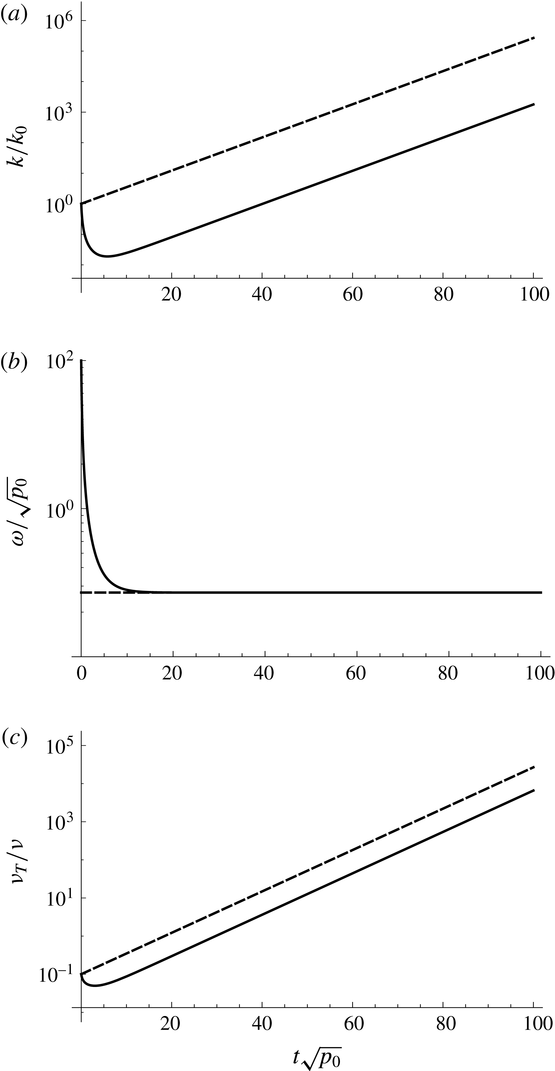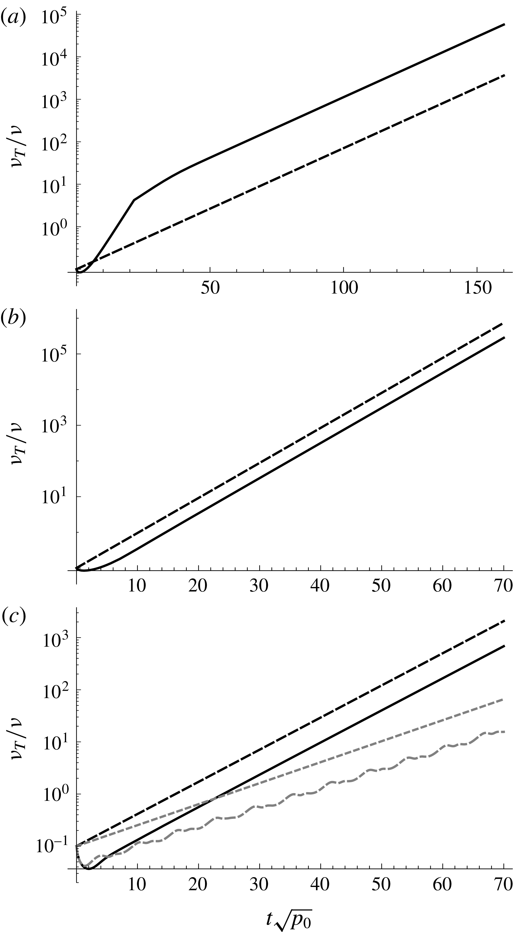Figure 1 shows the simulated temporal development of $k/k_{0}$ , $\unicode[STIX]{x1D714}/\sqrt{p_{0}}$ and $\unicode[STIX]{x1D708}_{T}/\unicode[STIX]{x1D708}$ . Included in the figure as the dashed lines are the predicted asymptotic exponential growth rates for $k$ and $\unicode[STIX]{x1D708}_{T}$ from the above analysis, as well as the predicted asymptotic value $\unicode[STIX]{x1D714}_{\infty }$ . As can be seen $\unicode[STIX]{x1D714}$ quickly tends towards $\unicode[STIX]{x1D714}_{\infty }$ , and once this occurs $k$ and $\unicode[STIX]{x1D708}_{T}$ (which were initially declining) start growing exponentially at precisely the growth rate $\unicode[STIX]{x1D6E4}_{\infty }$ predicted above.

Figure 1.

Simulated development (full lines) of (a) $k/k_{0}$ , (b) $\unicode[STIX]{x1D714}/\sqrt{p_{0}}$ and (c) $\unicode[STIX]{x1D708}_{T}/\unicode[STIX]{x1D708}$ for the Wilcox (Reference Wilcox1988) closure model. Dashed lines indicate predicted asymptotic exponential growth rates in (a) $k$ and (c) $\unicode[STIX]{x1D708}_{T}$ , as well as (b) the predicted asymptotic value $\unicode[STIX]{x1D714}=\unicode[STIX]{x1D714}_{\infty }$ .

2.4 Analysis of the modified Mayer & Madsen (Reference Mayer and Madsen2000) $k$ – $\unicode[STIX]{x1D714}$ model

In an effort to combat the unphysical growth of turbulence in their CFD simulation of breaking waves, Mayer & Madsen (Reference Mayer and Madsen2000) made an ad hoc modification of their production terms ( $P_{k}$ and $P_{\unicode[STIX]{x1D714}}$ , though they did not modify the eddy viscosity outside these terms) such that they were based on the vorticity, rather than the strain rate. They did not formally analyse the resulting turbulence closure model for stability, and this will therefore be investigated here. In the context of our simplified analysis, this ad hoc modification is equivalent to setting

(2.23) $$\begin{eqnarray}\displaystyle \tilde{\unicode[STIX]{x1D714}}=\tilde{\tilde{\unicode[STIX]{x1D714}}}=\frac{p_{0}}{p_{\unicode[STIX]{x1D6FA}}}\unicode[STIX]{x1D714} & & \displaystyle\end{eqnarray}$$

whence (2.15) and (2.16) become

(2.24) $$\begin{eqnarray}\displaystyle & \displaystyle \frac{\unicode[STIX]{x2202}k}{\unicode[STIX]{x2202}t}=\frac{k}{\unicode[STIX]{x1D714}}p_{\unicode[STIX]{x1D6FA}}-\unicode[STIX]{x1D6FD}^{\ast }\unicode[STIX]{x1D714}k, & \displaystyle\end{eqnarray}$$

(2.25) $$\begin{eqnarray}\displaystyle & \displaystyle \frac{\unicode[STIX]{x2202}\unicode[STIX]{x1D714}}{\unicode[STIX]{x2202}t}=\unicode[STIX]{x1D6FC}p_{\unicode[STIX]{x1D6FA}}-\unicode[STIX]{x1D6FD}\unicode[STIX]{x1D714}^{2}. & \displaystyle\end{eqnarray}$$

These are identical to (2.17) and (2.18), but with $p_{0}$ now replaced by $p_{\unicode[STIX]{x1D6FA}}$ . Hence, without requiring further analysis, it is evident that in this model $\unicode[STIX]{x1D714}$ will tend asymptotically to

(2.26) $$\begin{eqnarray}\displaystyle \unicode[STIX]{x1D714}_{\infty }=\sqrt{\frac{p_{\unicode[STIX]{x1D6FA}}\unicode[STIX]{x1D6FC}}{\unicode[STIX]{x1D6FD}}}\approx 2.71\sqrt{p_{\unicode[STIX]{x1D6FA}}} & & \displaystyle\end{eqnarray}$$

at which point the unstable growth rate for $k$ and $\unicode[STIX]{x1D708}_{T}$ will be

(2.27) $$\begin{eqnarray}\displaystyle \unicode[STIX]{x1D6E4}_{\infty }=(\unicode[STIX]{x1D6FD}-\unicode[STIX]{x1D6FC}\unicode[STIX]{x1D6FD}^{\ast })\sqrt{\frac{p_{\unicode[STIX]{x1D6FA}}}{\unicode[STIX]{x1D6FC}\unicode[STIX]{x1D6FD}}}\approx 0.125\sqrt{p_{\unicode[STIX]{x1D6FA}}}. & & \displaystyle\end{eqnarray}$$

Thus, even with this alteration, since the vorticity would never be exactly zero in a CFD model involving surface waves (due to both numerical error and/or imposed boundary conditions) the resulting model is still formally unconditionally unstable, although the asymptotic growth rate would be significantly reduced compared to the standard $k$ – $\unicode[STIX]{x1D714}$ model, since it is assumed that $p_{\unicode[STIX]{x1D6FA}}\ll p_{0}$ .

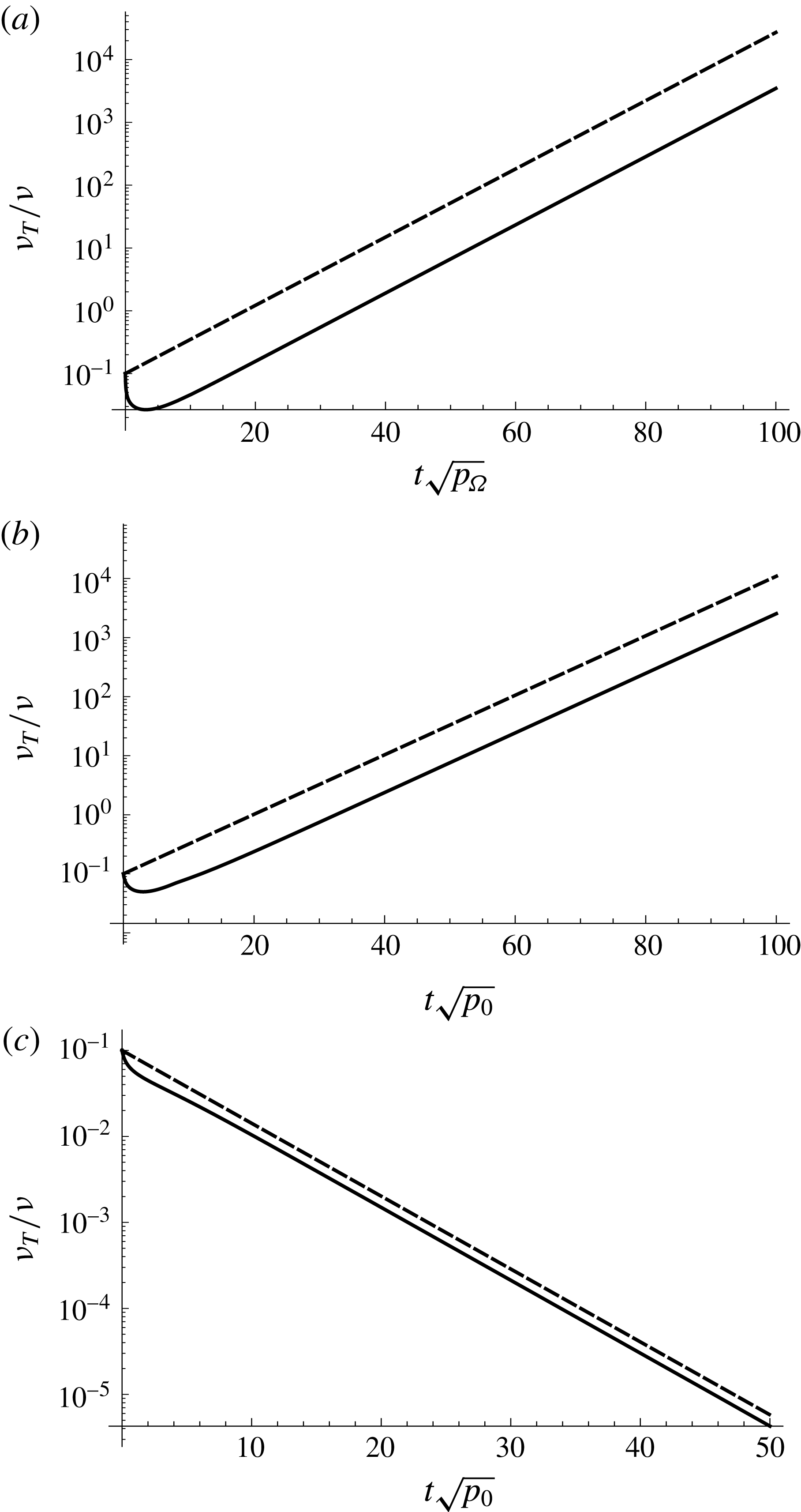
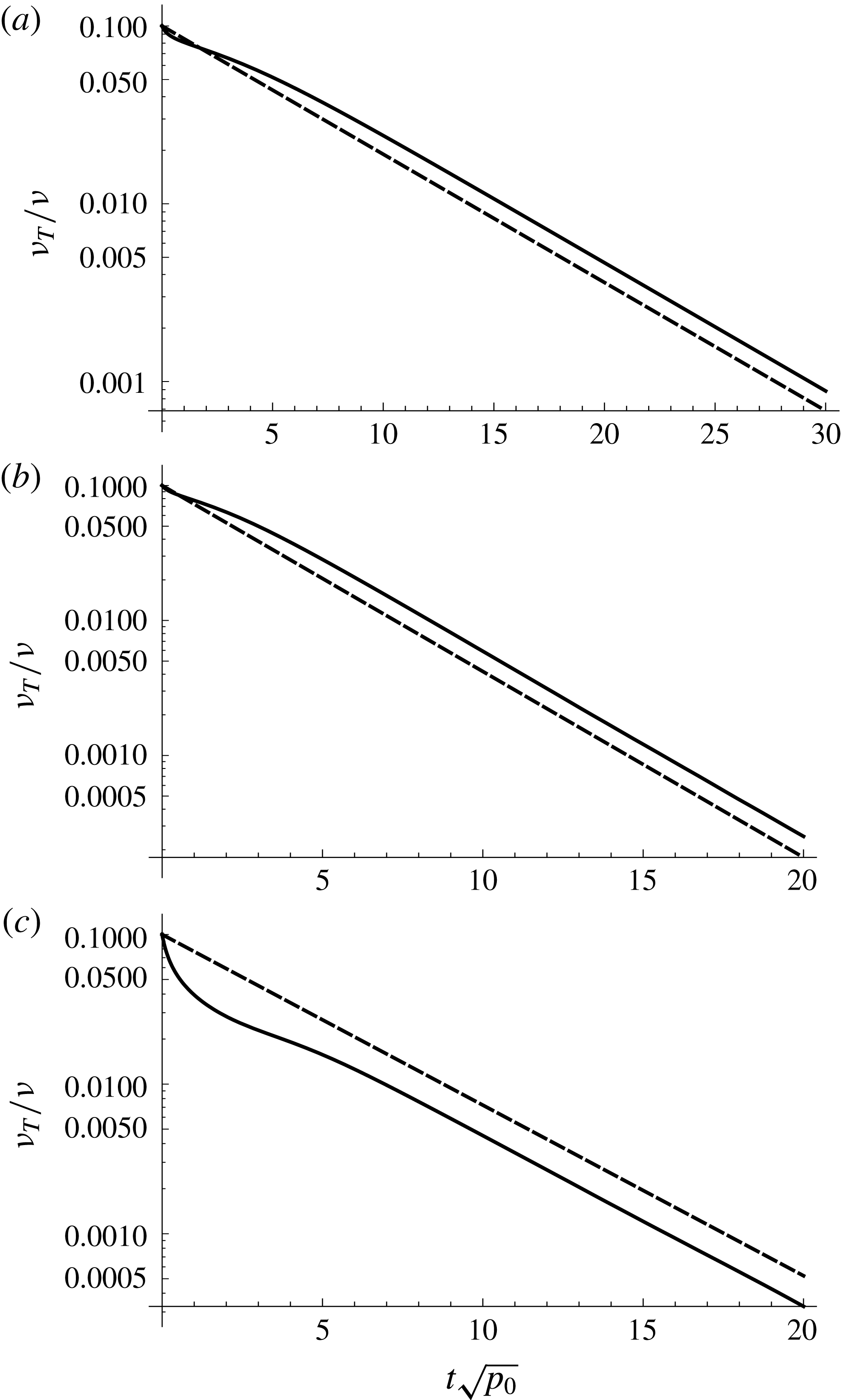
Independent confirmation of the analysis above is provided via numerical solution of the reduced governing equations, maintaining the same initial conditions as before and now with $p_{\unicode[STIX]{x1D6FA}}/p_{0}=0.01$ . The resulting evolution of the eddy viscosity is depicted in figure 2(a). Again this first declines, before ultimately growing exponentially at precisely the asymptotic rate predicted above.

Figure 2.

Simulated development of $\unicode[STIX]{x1D708}_{T}/\unicode[STIX]{x1D708}$ (full lines) compared to the predicted asymptotic exponential growth (dashed lines) for the (a) Mayer & Madsen (Reference Mayer and Madsen2000)  $k$ – $\unicode[STIX]{x1D714}$ closure, (b) Wilcox (Reference Wilcox2006)  $k$ – $\unicode[STIX]{x1D714}$ closure and (c) present $k$ – $\unicode[STIX]{x1D714}$ closure with $\unicode[STIX]{x1D706}_{1}=0$ and $\unicode[STIX]{x1D706}_{2}=0.05$ .

The ad hoc modification used by Mayer & Madsen (Reference Mayer and Madsen2000) represents an interesting first attempt to control the instability that they identified, and which was expanded upon in the preceding sub-section. Nevertheless, it cannot be considered a fundamentally viable solution for several reasons. First, although weaker, the model is still formally unconditionally unstable, as proved above. Second, Mayer & Madsen (Reference Mayer and Madsen2000) effectively utilized different $\tilde{\unicode[STIX]{x1D714}}$ in the production terms and in the eddy viscosity outside of these terms, which is in direct violation of the Boussinesq approximation (2.3); this is equivalent to simultaneously utilizing two different definitions of the Reynolds stress tensor $\unicode[STIX]{x1D70F}_{ij}$ . Third, it is again emphasized that the turbulence production term is theoretical in nature (derived directly from Reynolds averaging), and hence rightly ought to be based on the strain rate rather than the vorticity, at least if the standard Boussinesq approximation is utilized. While in simple uniform boundary layer flows these may be equal, in more complex flows they can be quite different. (For example, in the forthcoming simulation of spilling breaking waves we have found that they can differ by a factor of 1–10 in most of the surf zone.) Hence, in the context of surface waves this modification must be considered intrusive, resulting in a significantly altered turbulence production term that is applied globally i.e. even in sheared flow regions of primary interest (e.g. the surf zone), where the original model should be maintained. This is evidenced directly by the work of Jacobsen et al. (Reference Jacobsen, Fuhrman and Fredsøe2012), who utilized the modified production terms of Mayer & Madsen (Reference Mayer and Madsen2000) to simulate spilling breaking waves, and found that it was necessary to alter one of the fundamental closure coefficients in isolation (from $\unicode[STIX]{x1D6FC}=0.52$ to 0.4) to obtain reasonable undertow profiles. This is likewise problematic, since as shown e.g. in Wilcox (Reference Wilcox2006), the closure coefficients are carefully tuned, and are, among other things, related to the von Kármán constant $\unicode[STIX]{x1D705}$ according to

(2.28) $$\begin{eqnarray}\displaystyle \unicode[STIX]{x1D6FC}=\frac{\unicode[STIX]{x1D6FD}}{\unicode[STIX]{x1D6FD}^{\ast }}-\unicode[STIX]{x1D70E}\frac{\unicode[STIX]{x1D705}^{2}}{\sqrt{\unicode[STIX]{x1D6FD}^{\ast }}}. & & \displaystyle\end{eqnarray}$$

Hence, the alteration just mentioned corresponds to a model yielding $\unicode[STIX]{x1D705}\approx 0.482$ rather than the accepted $\unicode[STIX]{x1D705}\approx 0.4$ , and will therefore be inaccurate for simple steady uniform boundary layer flows. Indeed, it must be pointed out that (likely in recognition of some of the concerns presented above) Mayer & Madsen (Reference Mayer and Madsen2000) rightly concluded that ‘at this stage we do not recommend this modification as generally applicable and instead some new fundamental analysis and development seems necessary’, largely inspiring the present work.

2.5 Analysis of the Wilcox (Reference Wilcox2006) $k$ – $\unicode[STIX]{x1D714}$ model

As a third alternative, let us now similarly consider the stability of the Wilcox (Reference Wilcox2006) $k$ – $\unicode[STIX]{x1D714}$ closure model. In this closure model Wilcox (Reference Wilcox2006) added, among other things, a stress-limiting feature, such that

(2.29) $$\begin{eqnarray}\displaystyle \tilde{\unicode[STIX]{x1D714}}=\tilde{\tilde{\unicode[STIX]{x1D714}}}=\max \left[\unicode[STIX]{x1D714},\unicode[STIX]{x1D706}_{1}\sqrt{\frac{p_{0}}{\unicode[STIX]{x1D6FD}^{\ast }}}\right], & & \displaystyle\end{eqnarray}$$

where he suggested $\unicode[STIX]{x1D706}_{1}=7/8=0.875$ . This feature essentially limits the resulting eddy viscosity in regions where turbulence production exceeds the dissipation, and has been shown to result in larger separation bubbles and greatly improve incompressible and transonic flow predictions relative to models without this feature.

If the first argument in the limiter (2.29) dominates, then $\tilde{\unicode[STIX]{x1D714}}=\tilde{\tilde{\unicode[STIX]{x1D714}}}=\unicode[STIX]{x1D714}$ and the model becomes identical to that analysed in § 2.3, which was already proven to be unconditionally unstable in a nearly potential flow with finite $p_{0}$ . Alternatively, if the second (stress limiting) argument dominates, then (2.15) and (2.16) become

(2.30) $$\begin{eqnarray}\displaystyle & \displaystyle \frac{\unicode[STIX]{x2202}k}{\unicode[STIX]{x2202}t}=\frac{k}{\unicode[STIX]{x1D706}_{1}}\sqrt{\unicode[STIX]{x1D6FD}^{\ast }p_{0}}-\unicode[STIX]{x1D6FD}^{\ast }\unicode[STIX]{x1D714}k, & \displaystyle\end{eqnarray}$$

(2.31) $$\begin{eqnarray}\displaystyle & \displaystyle \frac{\unicode[STIX]{x2202}\unicode[STIX]{x1D714}}{\unicode[STIX]{x2202}t}=\frac{\unicode[STIX]{x1D6FC}\unicode[STIX]{x1D714}}{\unicode[STIX]{x1D706}_{1}}\sqrt{\unicode[STIX]{x1D6FD}^{\ast }p_{0}}-\unicode[STIX]{x1D6FD}\unicode[STIX]{x1D714}^{2}. & \displaystyle\end{eqnarray}$$

As before, setting the right-hand side of (2.31) equal to zero, we now find that $\unicode[STIX]{x1D714}$ will tend to the asymptotic value

(2.32) $$\begin{eqnarray}\displaystyle \unicode[STIX]{x1D714}_{\infty }=\frac{\unicode[STIX]{x1D6FC}}{\unicode[STIX]{x1D706}_{1}\unicode[STIX]{x1D6FD}}\sqrt{\unicode[STIX]{x1D6FD}^{\ast }p_{0}}\approx 2.52\sqrt{p_{0}}. & & \displaystyle\end{eqnarray}$$

Inserting this value for $\unicode[STIX]{x1D714}$ back into (2.30) then leads directly to linearized expressions of the form (2.21), where the unstable growth rate is

(2.33) $$\begin{eqnarray}\displaystyle \unicode[STIX]{x1D6E4}_{\infty }=\frac{(\unicode[STIX]{x1D6FD}-\unicode[STIX]{x1D6FC}\unicode[STIX]{x1D6FD}^{\ast })}{\unicode[STIX]{x1D706}_{1}\unicode[STIX]{x1D6FD}}\sqrt{\unicode[STIX]{x1D6FD}^{\ast }p_{0}}\approx 0.116\sqrt{p_{0}}. & & \displaystyle\end{eqnarray}$$

Hence, this model is likewise formally unconditionally unstable in the situation considered, although the stress limiter notably reduces the unstable growth rate slightly relative to the standard $k$ – $\unicode[STIX]{x1D714}$ model.

Independent confirmation of the analysis above is provided via numerical solution of (2.15) and (2.16) while invoking (2.29), maintaining the same initial conditions for $\unicode[STIX]{x1D714}$ and $\unicode[STIX]{x1D708}_{T}$ as before. The resulting evolution of the eddy viscosity is depicted in figure 2(b). As before, following the initial decline, the eddy viscosity grows exponentially at the rate predicted above.

2.6 Analysis of a new stabilized closure

In this section an elegant and simple solution to the instability considered above, which seems to widely plague most existing two-equation closure options (all that the authors have analysed), will be presented. We seek a solution to this long-standing problem that will be otherwise unintrusive i.e. such that the resulting model will default to an existing closure in sheared flow regions, while still formally curing the instability in regions of nearly potential flow. At the same time the solution should remain true to the theoretically based terms in the $k$ equation, maintain full consistency with the Boussinesq approximation, and not require alteration of any fundamental closure coefficients. We further aim for the solution to be readily adaptable to similarly stabilize other two-equation closures in wide use.

As just shown in § 2.5, the stress-limiting feature in the Wilcox (Reference Wilcox2006) model reduces the unstable growth rate, relative to the standard $k$ – $\unicode[STIX]{x1D714}$ model. Working within this established feature is therefore a natural place to attempt to remedy this problem. To both formally stabilize the model and generally improve the CFD simulation of surface waves with RANS models, we propose the following modifications to the stress-limiting features. First, we propose to generalize $\tilde{\tilde{\unicode[STIX]{x1D714}}}$ slightly such that:

(2.34) $$\begin{eqnarray}\displaystyle \tilde{\tilde{\unicode[STIX]{x1D714}}}=\max \left[\unicode[STIX]{x1D714},\unicode[STIX]{x1D706}_{1}\sqrt{\frac{p_{0}-p_{b}}{\unicode[STIX]{x1D6FD}^{\ast }}}\,\right], & & \displaystyle\end{eqnarray}$$

where we have included buoyancy production for potential two-phase (air and water) flow applications, for the sake of full consistency with (2.1). Obviously, this will not affect the formal stability of the model, as constant density (hence $p_{b}=0$ ) is assumed in the analysis. Second (and much more importantly in the present context), to formally stabilize the instability considered at length above, we propose the following modification to $\tilde{\unicode[STIX]{x1D714}}$ :

(2.35) $$\begin{eqnarray}\displaystyle \tilde{\unicode[STIX]{x1D714}}=\text{max}\left[\tilde{\tilde{\unicode[STIX]{x1D714}}},\unicode[STIX]{x1D706}_{2}\frac{\unicode[STIX]{x1D6FD}}{\unicode[STIX]{x1D6FD}^{\ast }\unicode[STIX]{x1D6FC}}\frac{p_{0}}{p_{\unicode[STIX]{x1D6FA}}}\unicode[STIX]{x1D714}\right], & & \displaystyle\end{eqnarray}$$

where $\unicode[STIX]{x1D706}_{2}\ll 1$ is an additional stress limiter coefficient, the physical meaning of which will be made explicitly clear in what follows. Note that the new addition to the limiter in (2.35) is, by design, unintrusive, as it will become active only in a region of nearly potential flow where $p_{0}\gg p_{\unicode[STIX]{x1D6FA}}$ . Moreover, note that (for single-phase incompressible flows) if $\unicode[STIX]{x1D706}_{2}=0$ the model becomes equivalent to the Wilcox (Reference Wilcox2006) model, whereas if $\unicode[STIX]{x1D706}_{1}=\unicode[STIX]{x1D706}_{2}=0$ this model becomes equivalent to the standard $k$ – $\unicode[STIX]{x1D714}$ model of Wilcox (Reference Wilcox1988). It is hence fully compatible with the other standard closures that have been specifically considered. (Note that to avoid any possibility of dividing by zero, the denominator in (2.35) can be implemented numerically as $p_{\unicode[STIX]{x1D6FA}}+\unicode[STIX]{x1D709}$ , where $\unicode[STIX]{x1D709}$ is a small number near machine precision, although we strictly analyse the form above for the sake of elegance.)

To demonstrate the formal asymptotic stability of the proposed new model, let us first repeat the above analysis of the standard Wilcox (Reference Wilcox1988) model (momentarily setting $\unicode[STIX]{x1D706}_{1}=0$ , hence $\tilde{\tilde{\unicode[STIX]{x1D714}}}=\unicode[STIX]{x1D714}$ ), but now with the new limiter active in $\tilde{\unicode[STIX]{x1D714}}$ . In this case, the $k$ equation (2.15) becomes

(2.36) $$\begin{eqnarray}\displaystyle \frac{\unicode[STIX]{x2202}k}{\unicode[STIX]{x2202}t}=\frac{\unicode[STIX]{x1D6FC}\unicode[STIX]{x1D6FD}^{\ast }}{\unicode[STIX]{x1D706}_{2}\unicode[STIX]{x1D6FD}}\frac{kp_{\unicode[STIX]{x1D6FA}}}{\unicode[STIX]{x1D714}}-\unicode[STIX]{x1D6FD}^{\ast }\unicode[STIX]{x1D714}k, & & \displaystyle\end{eqnarray}$$

whereas the $\unicode[STIX]{x1D714}$ equation from (2.16) remains equivalent to (2.18), and hence $\unicode[STIX]{x1D714}$ will ultimately evolve to $\unicode[STIX]{x1D714}_{\infty }$ from (2.20). Inserting this value into (2.36) leads to linearized expressions of the form (2.21), where the exponential growth rate is

(2.37) $$\begin{eqnarray}\displaystyle \unicode[STIX]{x1D6E4}_{\infty }=\sqrt{\frac{p_{0}\unicode[STIX]{x1D6FC}}{\unicode[STIX]{x1D6FD}}}\unicode[STIX]{x1D6FD}^{\ast }\left(\frac{p_{\unicode[STIX]{x1D6FA}}}{\unicode[STIX]{x1D706}_{2}p_{0}}-1\right). & & \displaystyle\end{eqnarray}$$

From this it can be seen that the new turbulence closure model will be formally stable (i.e.  $\unicode[STIX]{x1D6E4}_{\infty }\leqslant 0$ ) provided that

(2.38) $$\begin{eqnarray}\displaystyle \frac{p_{\unicode[STIX]{x1D6FA}}}{p_{0}}\leqslant \unicode[STIX]{x1D706}_{2}. & & \displaystyle\end{eqnarray}$$

This hence provides a clear physical meaning for the added stress limiter coefficient $\unicode[STIX]{x1D706}_{2}$ , as it defines the threshold of $p_{\unicode[STIX]{x1D6FA}}/p_{0}$ identifying a region as effectively potential flow. Note also that at the pure potential flow limit where $p_{\unicode[STIX]{x1D6FA}}=0$ , the growth rate is $\unicode[STIX]{x1D6E4}_{\infty }=-\unicode[STIX]{x1D6FD}^{\ast }\sqrt{p_{0}\unicode[STIX]{x1D6FC}/\unicode[STIX]{x1D6FD}}=-\unicode[STIX]{x1D6FD}^{\ast }\unicode[STIX]{x1D714}_{\infty }\approx -0.244\sqrt{p_{0}}$ , and any turbulent kinetic energy will decay similar to how it would in a quiescent fluid.

If instead, we repeat the analysis of the Wilcox (Reference Wilcox2006) model (now retaining $\unicode[STIX]{x1D706}_{1}$ ), then the $k$ equation will remain equivalent to (2.36), whereas the $\unicode[STIX]{x1D714}$ equation will be equivalent to (2.31), and hence $\unicode[STIX]{x1D714}$ will tend towards $\unicode[STIX]{x1D714}_{\infty }$ in (2.32). Inserting this value as a constant within (2.36) then similarly leads to linearized expressions of the form (2.21), where the unstable growth rate is

(2.39) $$\begin{eqnarray}\displaystyle \unicode[STIX]{x1D6E4}_{\infty }=\sqrt{p_{0}}\unicode[STIX]{x1D6FD}^{\ast }\left(\frac{p_{\unicode[STIX]{x1D6FA}}\unicode[STIX]{x1D706}_{1}}{p_{0}\unicode[STIX]{x1D706}_{2}\sqrt{\unicode[STIX]{x1D6FD}^{\ast }}}-\frac{\unicode[STIX]{x1D6FC}\sqrt{\unicode[STIX]{x1D6FD}^{\ast }}}{\unicode[STIX]{x1D706}_{1}\unicode[STIX]{x1D6FD}}\right). & & \displaystyle\end{eqnarray}$$

This will thus be stable provided that

(2.40) $$\begin{eqnarray}\displaystyle \frac{p_{\unicode[STIX]{x1D6FA}}}{p_{0}}\leqslant \unicode[STIX]{x1D706}_{2}\frac{\unicode[STIX]{x1D6FC}\unicode[STIX]{x1D6FD}^{\ast }}{\unicode[STIX]{x1D706}_{1}^{2}\unicode[STIX]{x1D6FD}}\approx 0.863\unicode[STIX]{x1D706}_{2}, & & \displaystyle\end{eqnarray}$$

where the standard coefficient values have been inserted. As the lead coefficient is near unity, it is seen that this further generalization does not greatly affect the previously mentioned physical interpretation of $\unicode[STIX]{x1D706}_{2}$ . Note also that once $\unicode[STIX]{x1D714}=\unicode[STIX]{x1D714}_{\infty }$ if $\unicode[STIX]{x1D706}_{1}<\sqrt{\unicode[STIX]{x1D6FC}\unicode[STIX]{x1D6FD}^{\ast }/\unicode[STIX]{x1D6FD}}\approx 0.813$ then the first argument will inevitably dominate in (2.34), and the threshold for stability will again be given by (2.38).

It should be noted that in uniform boundary layer flows $p_{0}=p_{\unicode[STIX]{x1D6FA}}$ , and thus the new limiter will be completely inactive. Moreover, in other more complicated sheared flow regions (e.g. both in the surf zone and the surface boundary layer region near the air–water interface) $p_{\unicode[STIX]{x1D6FA}}$ and $p_{0}$ will typically be the same order of magnitude, and the new limiter will similarly remain inactive. Hence, the new closure will, by design, effectively reduce to a standard closure, except in a region of nearly potential flow (clearly defined by the choice of $\unicode[STIX]{x1D706}_{2}$ ), where such existing standard methods are inherently unconditionally unstable. The value of $\unicode[STIX]{x1D706}_{2}$ should naturally be small, but also large enough to work for practical applications since $p_{\unicode[STIX]{x1D6FA}}$ can always be expected to have a small, but finite, value in the discretized world. Throughout this work $\unicode[STIX]{x1D706}_{2}=0.05$ is used to achieve such a balance.

The stabilization of the new model presented above has been confirmed via numerical simulation of (2.15) and (2.16) while invoking (2.34) and (2.35), maintaining the same initial conditions as before. An example (with $\unicode[STIX]{x1D706}_{1}=0$ and $\unicode[STIX]{x1D706}_{2}=0.05$ ) depicting the temporal evolution of the eddy viscosity is provided in figure 2(c). Consistent with the analysis above, exponential decay, rather than growth, is now observed. Thus, the new closure model should remain stable in a region of nearly potential flow with finite strain, in contrast to all of the other models considered previously.

2.7 Analysis of other existing closure models

The formal asymptotic stability of several other widely utilized two-equation turbulence closure models is similarly considered in appendix A. 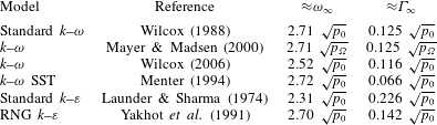These include: the $k$ – $\unicode[STIX]{x1D714}$ SST model originally formulated by Menter (Reference Menter1994), the standard $k$ – $\unicode[STIX]{x1D700}$ model of Launder & Sharma (Reference Launder and Sharma1974) and the RNG $k$ – $\unicode[STIX]{x1D700}$ model developed by Yakhot et al. (Reference Yakhot, Thangam, Speziale, Orszag and Gatski1991). It turns out that all of these basic two-equation models are similarly unconditionally unstable for the same conditions as analysed above. This is demonstrated analytically, as well as via independent numerical simulations of the reduced governing equations. 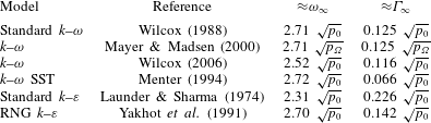The resulting asymptotic values for $\unicode[STIX]{x1D714}_{\infty }$ and the unstable growth rates $\unicode[STIX]{x1D6E4}_{\infty }$ for each of the pre-existing closure models analysed in the present work are summarized in table 1.

Table 1.

Summary of asymptotic $\unicode[STIX]{x1D714}$ values ( $\unicode[STIX]{x1D714}_{\infty }$ ) and unstable exponential growth rates ( $\unicode[STIX]{x1D6E4}_{\infty }$ ) for analysed existing two-equation turbulence closures.

Fortunately, and in line with the goals set forth above, these other widely utilized closure models can also be formally stabilized via simple modifications to their stress-limiting features, in a similar manner as presented in the preceding sub-section. The necessary modifications to stabilize each model are described in full detail in appendix A. With these modifications, asymptotic exponential decay (rather than growth) in the turbulent kinetic energy and eddy viscosity is proved analytically, as well as independently demonstrated through numerical simulation of the reduced modified model equations, similar to the above.

To avoid the potential for excessive and unphysical over-production of turbulence in nearly potential flow regions, it is recommended that these (or otherwise formally stabilized and unintrusive) modified closure models be utilized in any future CFD simulations of surface waves with two-equation RANS closure models, the significant and fundamental benefits of which will be demonstrated in the next section.

3.1 Model description

For the purposes of CFD simulation, surface water waves will be considered in the context of two-phase (air and water) flow. For this purpose the turbulence model defined by (2.1) and (2.2) will be used to close a CFD model solving incompressible RANS equations

(3.1) $$\begin{eqnarray}\displaystyle \frac{\unicode[STIX]{x2202}\unicode[STIX]{x1D70C}u_{i}}{\unicode[STIX]{x2202}t}+u_{j}\frac{\unicode[STIX]{x2202}\unicode[STIX]{x1D70C}u_{i}}{\unicode[STIX]{x2202}x_{j}}=-\frac{\unicode[STIX]{x2202}p^{\ast }}{\unicode[STIX]{x2202}x_{i}}-g_{j}x_{j}\frac{\unicode[STIX]{x2202}\unicode[STIX]{x1D70C}}{\unicode[STIX]{x2202}x_{i}}+\frac{\unicode[STIX]{x2202}}{\unicode[STIX]{x2202}x_{j}}(2\unicode[STIX]{x1D707}S_{ji}+\unicode[STIX]{x1D70F}_{ij}), & & \displaystyle\end{eqnarray}$$

and the local continuity equation

(3.2) $$\begin{eqnarray}\displaystyle \frac{\unicode[STIX]{x2202}u_{i}}{\unicode[STIX]{x2202}x_{i}}=0. & & \displaystyle\end{eqnarray}$$

In the above $p^{\ast }$ is the pressure in excess of hydrostatic. A scalar field $\unicode[STIX]{x1D6FE}$ is used to track the two fluids, where $\unicode[STIX]{x1D6FE}=0$ represents pure air and $\unicode[STIX]{x1D6FE}=1$ pure water, with any intermediate value representing a mixture. The distribution of $\unicode[STIX]{x1D6FE}$ is governed by an advection equation

(3.3) $$\begin{eqnarray}\displaystyle \frac{\unicode[STIX]{x2202}\unicode[STIX]{x1D6FE}}{\unicode[STIX]{x2202}t}+u_{j}\frac{\unicode[STIX]{x2202}u_{i}\unicode[STIX]{x1D6FE}}{\unicode[STIX]{x2202}x_{j}}+u_{j}^{r}\frac{\unicode[STIX]{x2202}u_{i}^{r}\unicode[STIX]{x1D6FE}(1-\unicode[STIX]{x1D6FE})}{\unicode[STIX]{x2202}u_{j}^{r}}=0, & & \displaystyle\end{eqnarray}$$

where $u_{j}^{r}$ is a relative velocity used to compress the interface, as documented in Berberovic et al. (Reference Berberovic, van Hinsberg, Jakirlic, Roisman and Tropea2009). Any fluid property $\unicode[STIX]{x1D6F7}$ in the flow is assumed to be given by

(3.4) $$\begin{eqnarray}\displaystyle \unicode[STIX]{x1D6F7}=\unicode[STIX]{x1D6FE}\unicode[STIX]{x1D6F7}_{water}+(1-\unicode[STIX]{x1D6FE})\unicode[STIX]{x1D6F7}_{air}. & & \displaystyle\end{eqnarray}$$

The governing equations are solved within the open-source CFD environment OpenFOAM (version foam-extend 3.1), making use of the waves2FOAM toolbox developed by Jacobsen et al. (Reference Jacobsen, Fuhrman and Fredsøe2012) for wave generation/absorption or specification of initial conditions. This toolbox is built upon the widely used interFoam solver, which utilizes the volume of fluid method (VOF). Unless stated otherwise, in both the RANS (3.1), the advection of $\unicode[STIX]{x1D6FE}$ (3.3) and the turbulence model equations (2.1) and (2.2) time derivatives are discretized using a first-order implicit Euler scheme. Convection terms are discretized using a blend of central difference and upwind schemes, depending on the ratio of successive gradients. Remaining schemes are second-order accurate central difference schemes. For further details on this solver the interested reader is referred to Deshpande, Anumolu & Trujillo (Reference Deshpande, Anumolu and Trujillo2012). In all forthcoming cases the time step has been adjusted such that a maximum Courant number $Co=|u_{i}|\unicode[STIX]{x0394}t/\unicode[STIX]{x0394}x_{i}=0.05$ is maintained at all times. Such a low Courant number is not typical but this ensures accurate velocity kinematics and enables nearly constant form propagation of wave trains for long durations, as shown by Larsen, Fuhrman & Roenby (Reference Larsen, Fuhrman and Roenby2018b ). Boundary conditions will be clarified on a case-by-case basis in what follows.

3.2 Simulation of a simple progressive wave train

In this section computed results will be presented for the long-term propagation of a periodic surface wave train. This is perhaps the simplest of computational wave problems, and is a test that should ideally be passed by CFD models prior to their application on more complicated problems. As an initial condition, a numerically exact streamfunction wave (potential flow) solution of Fenton (Reference Fenton1988) is specified, with no net volume flux, and with period $T=2$  s, wave height $H=0.125$  m and water depth $h=0.4$  m (hence $k_{w}h=0.664$ and $k_{w}H=0.207$ ). It should be noted that this wave is the same as that generated for the forthcoming simulation of the Ting & Kirby (Reference Ting and Kirby1994) spilling breaker experiments. Being intermediately deep and moderately nonlinear, these wave conditions are indeed well suited for generic study.

The computational domain is discretized into regular cells having horizontal and vertical size $\unicode[STIX]{x0394}x=\unicode[STIX]{x0394}z=0.01$  m (corresponding to $H/\unicode[STIX]{x0394}z=12.5$ cells per wave height). This resolution has been experienced to be sufficient for the accurate propagation of this specific wave in a laminar set-up. This mesh also maintains an aspect ratio $\unicode[STIX]{x0394}x/\unicode[STIX]{x0394}z=1$ , which can be important for accuracy, as noted by Jacobsen et al. (Reference Jacobsen, Fuhrman and Fredsøe2012), Jacobsen et al. (Reference Jacobsen, Fredsøe and Jensen2014) and Roenby et al. (Reference Roenby, Larsen, Bredmose and Jasak2017). The computational domain spans a single wavelength, making use of periodic lateral boundaries. At the bottom boundary a slip condition is applied. This is primarily for canonical demonstration purposes, making the computational situation as close to potential flow as possible, such that a turbulence closure model should ideally not influence the physics of the wave propagation.

To demonstrate the performance of the proposed new turbulence closure relative to standard approaches, we will compare computed results from the standard Wilcox (Reference Wilcox1988) $k$ – $\unicode[STIX]{x1D714}$ model (with the buoyancy production term also included in (2.1), henceforth taken as granted) with those from our new closure with $\unicode[STIX]{x1D706}_{1}=0$ and $\unicode[STIX]{x1D706}_{2}=0.05$ . All other model settings are kept identical. We initially set $\unicode[STIX]{x1D714}=\unicode[STIX]{x1D714}_{\infty }=2.71\sqrt{p_{0}}$ , where $p_{0}=0.66~\text{s}^{-2}$ is the depth- and period-averaged value computed from the initial conditions, and with $k=k_{0}=\unicode[STIX]{x1D714}_{\infty }\unicode[STIX]{x1D708}$ to initially yield $\unicode[STIX]{x1D708}_{T}/\unicode[STIX]{x1D708}=1$ . This is intended as a direct test of the preceding simplified analysis in an actual surface wave computation, where the standard closure should exhibit unstable behaviour from the outset, whereas the proposed new closure should remain stable indefinitely. We consider the initial condition for $\unicode[STIX]{x1D714}$ above to be most sensible in the present context, since as shown previously, it will always tend to approximately this value in the potential flow region beneath waves.

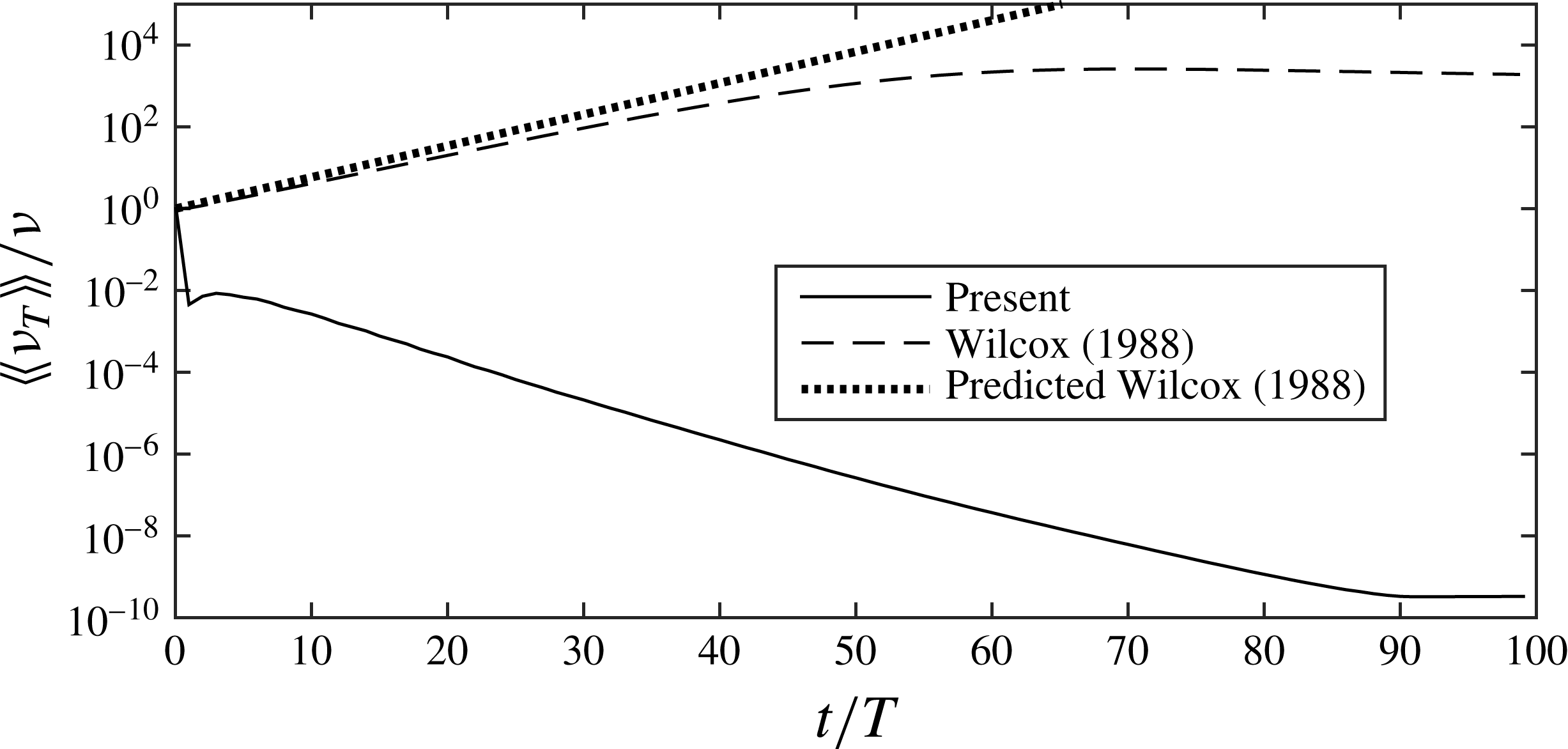
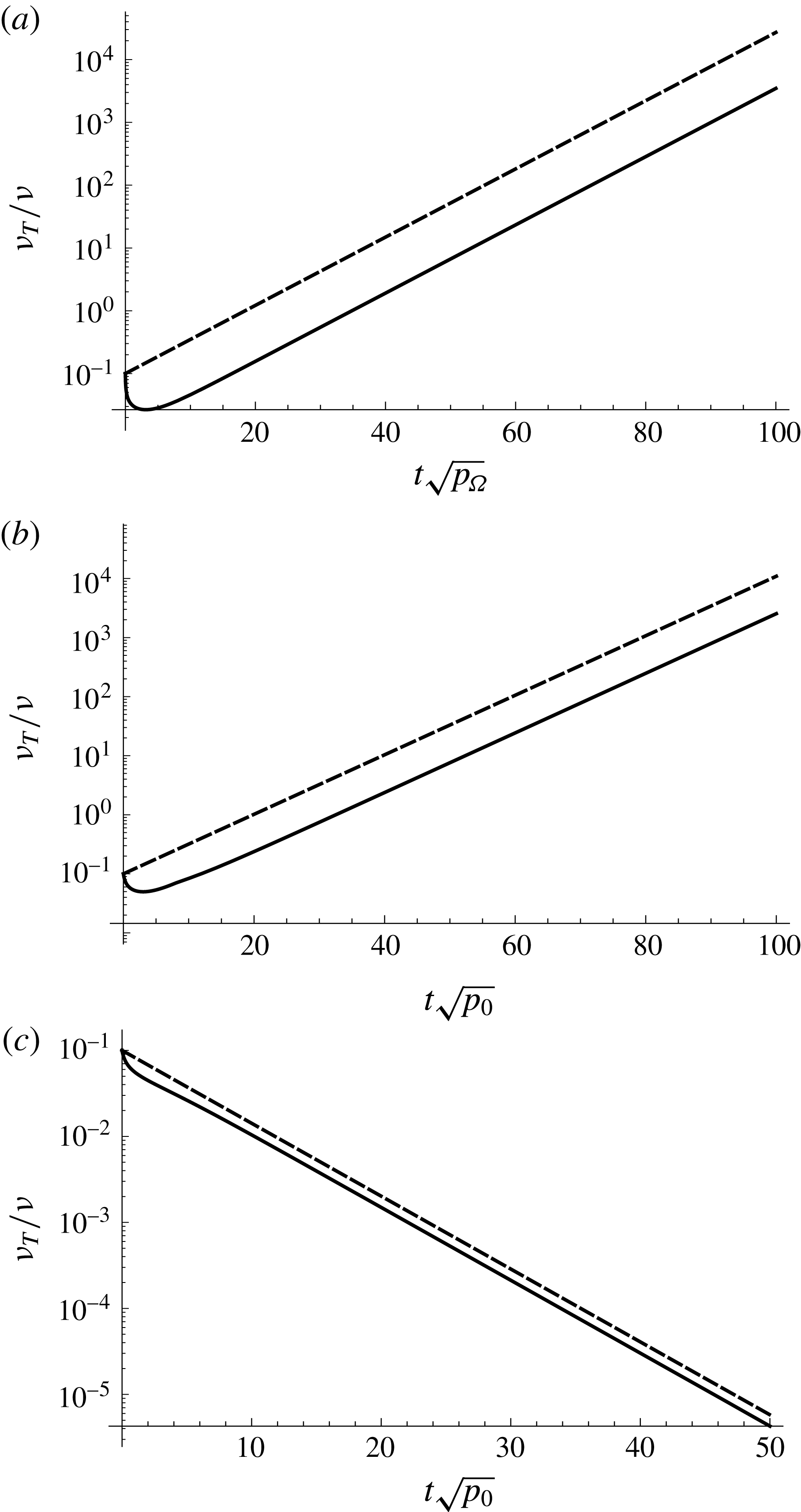
Figure 3 shows the computed temporal development of the (depth- and period-averaged) non-dimensional eddy viscosity $\langle \langle \unicode[STIX]{x1D708}_{T}\rangle \rangle /\unicode[STIX]{x1D708}$ with both closure models considered. Included in the figure (dashed line) is also the predicted development of $\langle \langle \unicode[STIX]{x1D708}_{T}\rangle \rangle /\unicode[STIX]{x1D708}=\exp (\unicode[STIX]{x1D6E4}_{\infty }t)$ with the growth rate from (2.22). Figure 3 clearly shows that the Wilcox (Reference Wilcox1988) $k$ – $\unicode[STIX]{x1D714}$ model is indeed initially unstable, resulting in an exponentially growing eddy viscosity (hence also $k$ ) that ultimately becomes several orders of magnitude larger than the kinematic viscosity, before eventually levelling off. The computed exponential growth rate is near that expected based on the simplified analysis, which has neglected several terms. It is emphasized that the growth of turbulence does not come from the bottom boundary layer, which is non-existent as a slip condition has again been used. Nor does it stem from the free surface, where the buoyancy production term in (2.7) suppresses turbulent kinetic energy in this region. Rather, it is due to the instability of the potential flow region, as confirmed via the close match with the theoretical growth rate. In contrast, also consistent with the preceding analysis, our new modified closure remains stable, with the eddy viscosity quickly decaying to physically insignificant levels.

Figure 3.

Computed temporal development of the depth- and period-averaged eddy viscosity beneath a periodic wave train using the present $k$ – $\unicode[STIX]{x1D714}$ closure model with $\unicode[STIX]{x1D706}_{1}=0$ and $\unicode[STIX]{x1D706}_{2}=0.05$ (full line), the Wilcox (Reference Wilcox1988)  $k$ – $\unicode[STIX]{x1D714}$ model (dashed line) as well as the predicted development from (2.22) (dotted line).

Figure 4.

Computed time series of surface elevations in the simulation of a periodic wave train using (a) the standard Wilcox (Reference Wilcox1988)  $k$ – $\unicode[STIX]{x1D714}$ model and (b) the proposed new closure model with $\unicode[STIX]{x1D706}_{1}=0$ and $\unicode[STIX]{x1D706}_{2}=0.05$ . The horizontal dashed lines represent the crest and trough levels of the initial wave, for comparison. (These results use a ‘diffusive balance’ in the schemes, as detailed in Larsen et al. Reference Larsen, Fuhrman and Roenby2018b .)

The eventual levelling off of the eddy viscosity with the standard $k$ – $\unicode[STIX]{x1D714}$ of Wilcox (Reference Wilcox1988) can be explained as due to declining wave heights, which are a direct consequence of the unphysical growth of the turbulent kinetic energy and eddy viscosity. These eventually reach levels that are sufficiently high to cause unphysical turbulent diffusion of the wave, with energy thus being extracted from the mean flow. 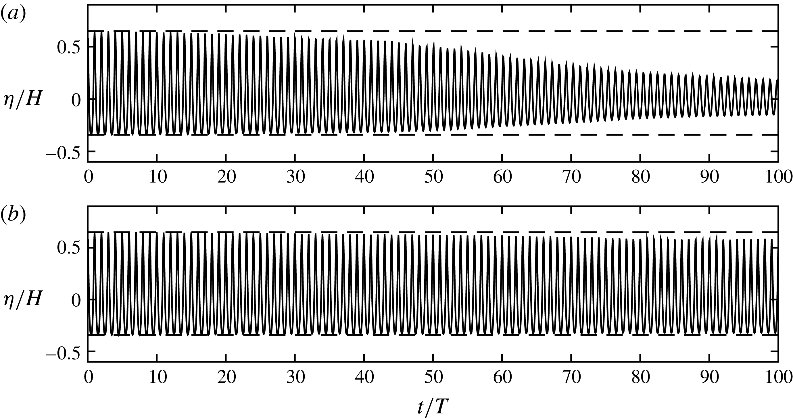As a result of the decreased wave height the turbulence production quantity $p_{0}$ is likewise reduced. This can be seen from the surface elevation time series depicted in figure 4(a), where the waves begin to decline after only $t\approx 20T$ . The decay in wave height is similar to what was shown by Mayer & Madsen (Reference Mayer and Madsen2000) and Devolder et al. (Reference Devolder, Rauwoens and Troch2017). In contrast, the wave evolution computed with the new stabilized closure maintains a nearly constant wave height, as seen from figure 4(b). The slight decay seen is clearly due to minor numerical diffusion associated with the numerical scheme, and not in any way related to the new turbulence closure, as it has effectively switched itself off. This is clear from the previously mentioned extremely small eddy viscosity in figure 3, as well as through comparison with an additional (otherwise identical) simulation with the turbulence model switched off entirely, which results in visually identical behaviour (not directly shown here for the sake of brevity). Note that we have also made other, similar, simulations as above, with $0.02\leqslant \unicode[STIX]{x1D706}_{2}\leqslant 0.1$ , which result in similar surface elevations as in figure 4(b).

This example demonstrates how the instability identified by Mayer & Madsen (Reference Mayer and Madsen2000), and which is inherent in standard two-equation turbulence closure models as shown herein, can manifest in their rather spectacular failure in even the simplest of surface wave computations. The comparison above likewise demonstrates that such failure can be avoided entirely by employing the simple new (stabilized) closure proposed herein.

3.3 Simulation of spilling breaking waves

As a follow-up to the preceding example, let us now consider simulations of the spilling breaking wave experiment of Ting & Kirby (Reference Ting and Kirby1994), to demonstrate the performance of the new model in a more physically complex situation. We focus here exclusively on their spilling, rather than plunging, case as it is these incoming wave conditions where the over-production of turbulence has consistently been observed in prior studies. Quantitatively the reason for this can be explained by equation (2.13) which yields $\langle \langle p_{0}\rangle \rangle =0.55~\text{s}^{-2}$ and $\langle \langle p_{0}\rangle \rangle =0.08~\text{s}^{-2}$ for their spilling and plunging cases respectively, i.e. a much lower turbulence production and hence unstable growth rate for the plunging case. It is emphasized that the strength of the instability does not strictly depend on the breaker type (which also depends on the slope encountered), but rather only on the characteristics of the incoming waves. (Note that the interested reader can find results from similar simulations utilizing our stabilized closure on the plunging breaking case in the PhD thesis of Larsen Reference Larsen2018.)

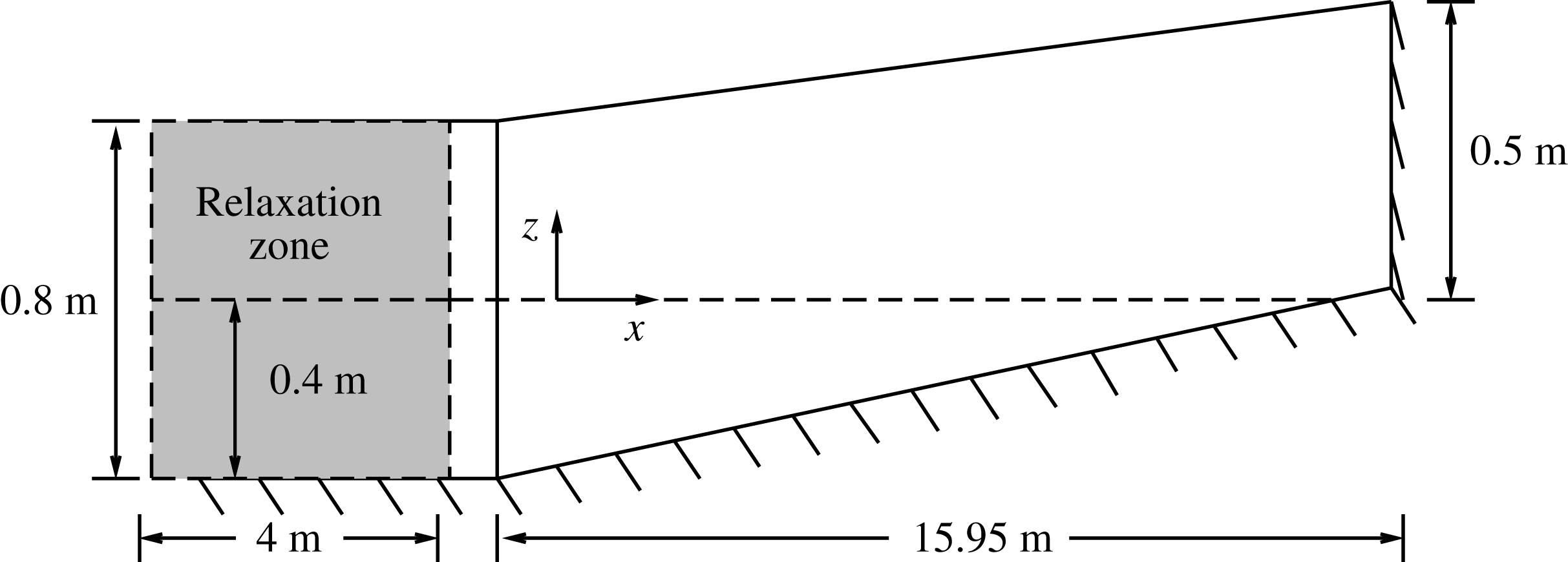
The model domain for these simulations consists of a flat region having water depth $h=0.4$  m, connected to a region having constant 1:35 slope. For these simulations, the same waves as considered previously ( $T=2$  s and $H=0.125$  m with zero net volume flux; $k_{w}h=0.664$ and $k_{w}H=0.207$ ) are generated on the horizontal bed. At the left inlet boundary a relaxation zone of 4 m is used, which serves to absorb any waves reflected by the slope, thus the incoming waves do not change over time. In figure 5 a layout of the computational domain is seen. For the purposes of consistent comparison, the origin is positioned at the same depth ( $h=0.38$  m) as in the experiments. No roughness was indicated in the experiment, but it was stated that the bed was made of plywood, and therefore the model bed is assigned a Nikuradse equivalent sand roughness $k_{s}=10^{-4}$  m.

Figure 5.

Layout of the computational domain for the simulation of the spilling breaking wave experiments of Ting & Kirby (Reference Ting and Kirby1994).

The initial condition for $\unicode[STIX]{x1D714}$ is again taken as $\unicode[STIX]{x1D714}=\unicode[STIX]{x1D714}_{\infty }=2.71\sqrt{p_{0}}$ , with $p_{0}$ calculated from (2.13) and with $k=k_{0}=0.1\unicode[STIX]{x1D714}_{\infty }\unicode[STIX]{x1D708}$ such that $\unicode[STIX]{x1D708}_{T}/\unicode[STIX]{x1D708}=0.1$ (this is one order of magnitude below that used in the previous progressive wave train test case in § 3.2). In contrast to the previous idealized simulation in § 3.2, a no-slip boundary condition is imposed at the bottom, meaning that a wave boundary layer will now develop near the bed, as in reality. Turbulence quantities in the first cell near the bottom are prescribed using the generalized wall functions presented in Fuhrman et al. (Reference Fuhrman, Baykal, Sumer, Jacobsen and Fredsoe2014), which build upon the generalized van Driest profile of Cebeci & Chang (Reference Cebeci and Chang1978). These wall functions have been used successfully in the simulation of various scour processes, see e.g. Baykal et al. (Reference Baykal, Sumer, Fuhrman, Jacobsen and Fredsøe2015), Bayraktar et al. (Reference Bayraktar, Ahmad, Larsen, Carstensen and Fuhrman2016), Larsen, Fuhrman & Sumer (Reference Larsen, Fuhrman and Sumer2016), Larsen et al. (Reference Larsen, Fuhrman, Baykal and Sumer2017) and Larsen et al. (Reference Larsen, Arbøll, Frigaard, Carstensen and Fuhrman2018a ), and allow for near-bed cells to lie in either the logarithmic or viscous sub-layer. On the flat region the domain is discretized into cells with $\unicode[STIX]{x0394}x=\unicode[STIX]{x0394}z=0.01$  m, and on the slope the mesh is gradually refined towards the shore while keeping a constant aspect ratio of unity. At the right end of the domain the cells have a size $\unicode[STIX]{x0394}x=\unicode[STIX]{x0394}z=0.0063$  m. Near the bed, layers of cells are refined in the vertical direction with near-bed cells having height $\unicode[STIX]{x0394}z=7.5\times 10^{-4}$  m. This ensures that $\unicode[STIX]{x0394}z^{+}=\unicode[STIX]{x0394}zU_{f}/\unicode[STIX]{x1D708}<30$ during the simulation, with $U_{f}$ being the friction velocity.

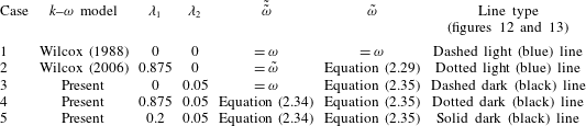
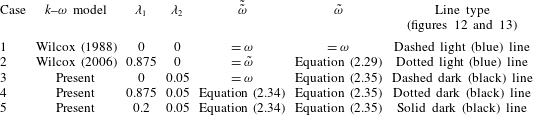
For the sake of systematic comparison, simulations of these experiments will be considered using five different turbulence closure variants. These correspond to: (Case 1) the standard Wilcox (Reference Wilcox1988) $k$ – $\unicode[STIX]{x1D714}$ model, (Case 2) the Wilcox (Reference Wilcox2006) $k$ – $\unicode[STIX]{x1D714}$ model, as well as three variants of the proposed modified $k$ – $\unicode[STIX]{x1D714}$ closure with fixed $\unicode[STIX]{x1D706}_{2}=0.05$ and: (Case 3) $\unicode[STIX]{x1D706}_{1}=0$ , (Case 4) $\unicode[STIX]{x1D706}_{1}=0.875$ and (Case 5) $\unicode[STIX]{x1D706}_{1}=0.2$ . The $\unicode[STIX]{x1D706}_{1}$ values in Cases 3 and 4 correspond to those associated with the models of Wilcox (Reference Wilcox1988) and Wilcox (Reference Wilcox2006) (thus allowing direct comparison) i.e. Cases 3 and 4 correspond to stabilized versions of Cases 1 and 2, respectively. Case 5 utilizes an intermediate value for $\unicode[STIX]{x1D706}_{1}$ , more in line with equation (9) of Durbin (Reference Durbin2009) (corresponding to $\unicode[STIX]{x1D706}_{1}=0.26$ ). For ultimate clarity, the parameter settings used in these five cases are listed in table 2. We shall henceforth refer to these simulations by their case number, as indicated in table 2 and in the text immediately above.

Table 2.

Summary of parameters used in the five different simulations of the Ting & Kirby (Reference Ting and Kirby1994) spilling breaking wave experiment.

Figure 6.

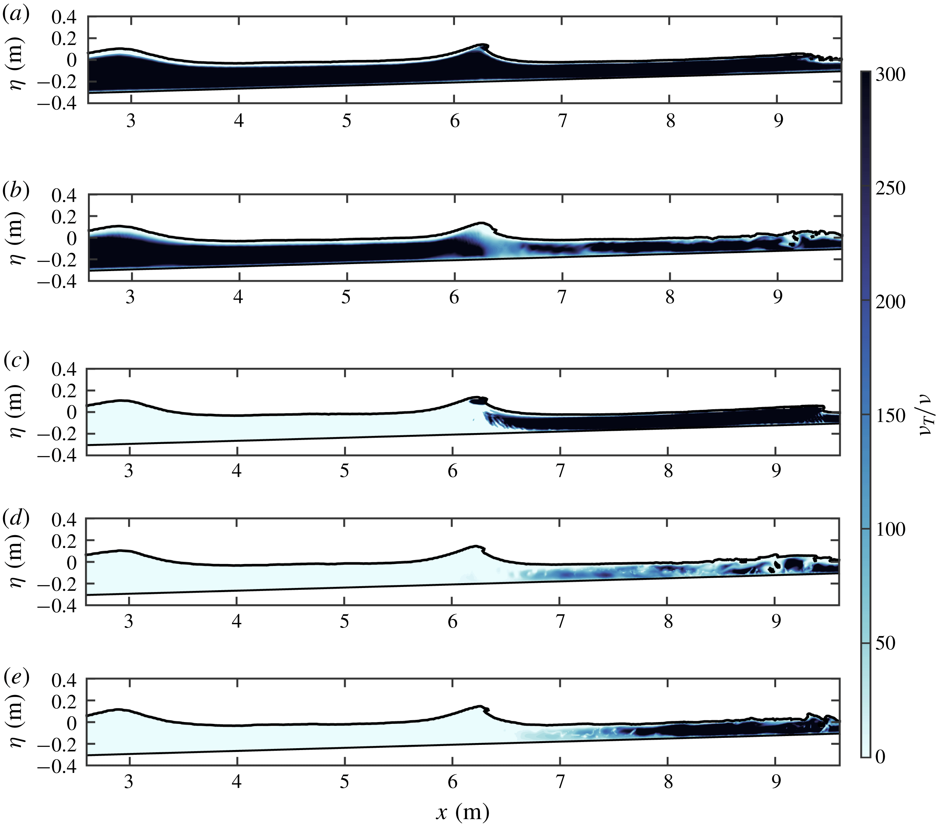
Snapshots of $\unicode[STIX]{x1D708}_{T}/\unicode[STIX]{x1D708}$ at $t/T=100$ with the wave right at breaking computed with the (a) standard Wilcox (Reference Wilcox1988) $k$ – $\unicode[STIX]{x1D714}$ model (Case 1), (b) Wilcox (Reference Wilcox2006)  $k$ – $\unicode[STIX]{x1D714}$ model (Case 2) and (c–e) present stabilized $k$ – $\unicode[STIX]{x1D714}$ closure model (respectively, Cases 3–5), where parameters for each case are indicated in table 2. The free surface and bottom are marked by solid lines.

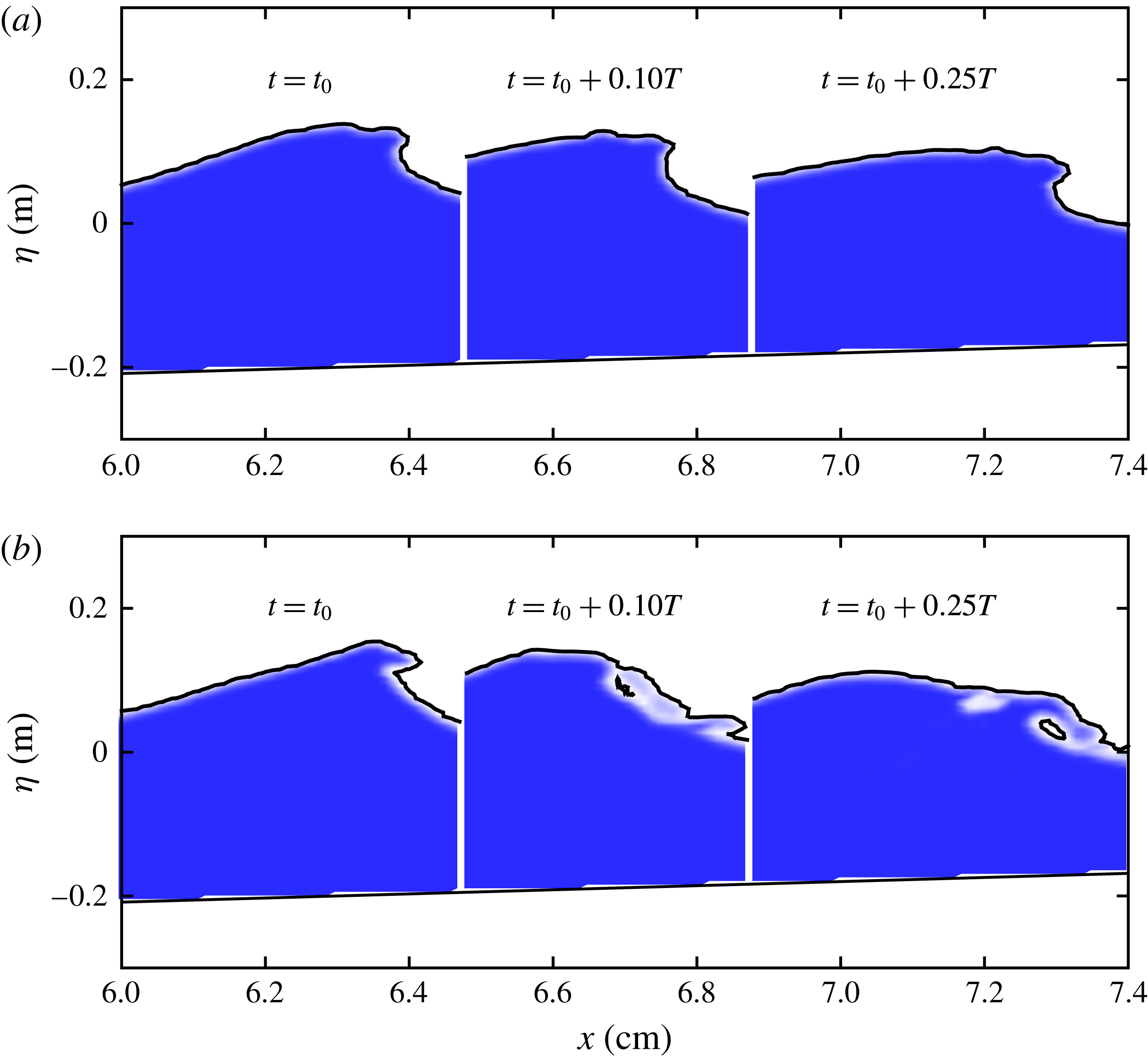
Figure 6 shows computed snapshots depicting the surface and non-dimensional eddy viscosity $\unicode[STIX]{x1D708}_{T}/\unicode[STIX]{x1D708}$ from each of the five model variants mentioned above, following a long simulation time of 100 periods, such that steady (repeatable) conditions have effectively been reached. (As an indication of simulation time, each run requires approximately three weeks when simulated in parallel on eight modern processors.) Each plot is frozen at an instant where the wave is very close to breaking, such that the location of the surf zone is evident (beginning approximately at $x=x_{b}=6.4$  m). As can be seen, both the standard Wilcox (Reference Wilcox1988) (Case 1, figure 6 a) and the Wilcox (Reference Wilcox2006) $k$ – $\unicode[STIX]{x1D714}$ models (Case 2, figure 6 b) result in uniformly high eddy viscosity (orders of magnitude larger than $\unicode[STIX]{x1D708}$ ), even in the pre-breaking region. These high values are in no way physical, as in real waves significant turbulence should not be expected prior to breaking, see e.g. the measured turbulence levels from Ting & Kirby (Reference Ting and Kirby1994) and van der A et al. (Reference van der A, van der Zanden, O’Donoghue, Hurther, Caceres, McLelland and Ribberink2017), the particle image velocimetry (PIV) experiments of Chang & Liu (Reference Chang and Liu1998), Grue & Jensen (Reference Grue and Jensen2006), Kimmoun & Branger (Reference Kimmoun and Branger2007) and Belden & Techet (Reference Belden and Techet2011) or the dye experiment of Duncan et al. (Reference Duncan, Qiao, Philomin and Wenz1999). Rather, these high values are again an artefact related to the inherent instability of these models in the nearly potential flow regions which are prevalent leading up to the surf zone. Conversely, regardless of the value of $\unicode[STIX]{x1D706}_{1}$ , the three results using the proposed new stabilized closure (figure 6 c–e corresponding to Cases 3–5) predict negligible eddy viscosity in the bulk region beneath the waves prior to breaking; significant eddy viscosity with these stabilized models is rightly confined to the near-bed boundary layer and surf zone, demonstrating a clear and qualitative correction over existing models. Figure 6 is hence a clear demonstration of how, due to their inherent instability, existing standard turbulence closure models in wide use can result in severely polluted results prior to wave breaking, often the very phenomenon of interest in CFD studies where such models are employed. This figure likewise definitively demonstrates that the new stabilized closure model proposed herein eliminates this problem altogether.

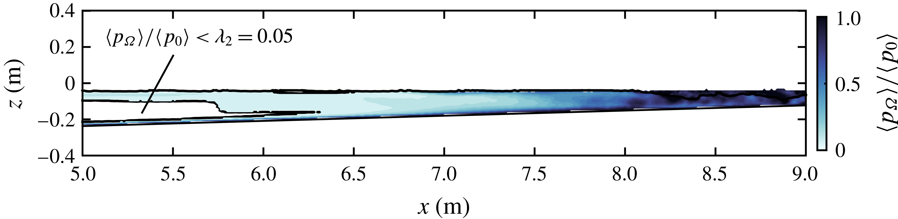
To provide further details on the computed vorticity-to-strain ratios found in the present simulations, figure 7 depicts $\langle p_{\unicode[STIX]{x1D6FA}}\rangle /\langle p_{0}\rangle$ beneath trough level, averaged over $60<t/T<120$ for Case 5 (as an example of our stabilized approach). The colour scheme in this figure has been chosen such that the white region corresponds to nearly potential flow i.e. where $\langle p_{\unicode[STIX]{x1D6FA}}\rangle /\langle p_{0}\rangle <\unicode[STIX]{x1D706}_{2}=0.05$ , and the new stabilizing limiter would thus be (on average) active. Conversely, coloured (shaded) regions correspond to sheared flow where this threshold value is exceeded, and the new limiter would essentially be off. It is seen that the location where the nearly potential flow region ends closely coincides to the beginning of the surf zone (again, beginning approximately at $x=x_{b}=6.4$  m), as should be expected. Prior to breaking the proposed limiter is typically active only in the nearly potential flow core region in the middle of the water column, whereas it is inactive in the sheared regions below and above, respectively corresponding to boundary layer regions which form where the water interacts with the bed and air (note that $\langle p_{\unicode[STIX]{x1D6FA}}\rangle$ and $\langle p_{0}\rangle$ are the same order of magnitude in these regions). This figure also clearly shows that in the surf zone $\langle p_{\unicode[STIX]{x1D6FA}}\rangle$ and $\langle p_{0}\rangle$ are generally within an order of magnitude of one another, although they are often far from equal. In the inner surf zone they are even more similar and are typically within a factor of two. This figure, in conjunction with the eddy viscosity plots in figure 6, thus further confirms that (as designed) the new limiter is primarily only active in the nearly potential flow region prior to breaking, while essentially remaining passive in the surf zone and other sheared regions.

Figure 7.

Computed $\langle p_{\unicode[STIX]{x1D6FA}}\rangle /\langle p_{0}\rangle$ below trough level for Case 5. The region where $\langle p_{\unicode[STIX]{x1D6FA}}\rangle /\langle p_{0}\rangle <\unicode[STIX]{x1D706}_{2}=0.05$ is indicated in white.

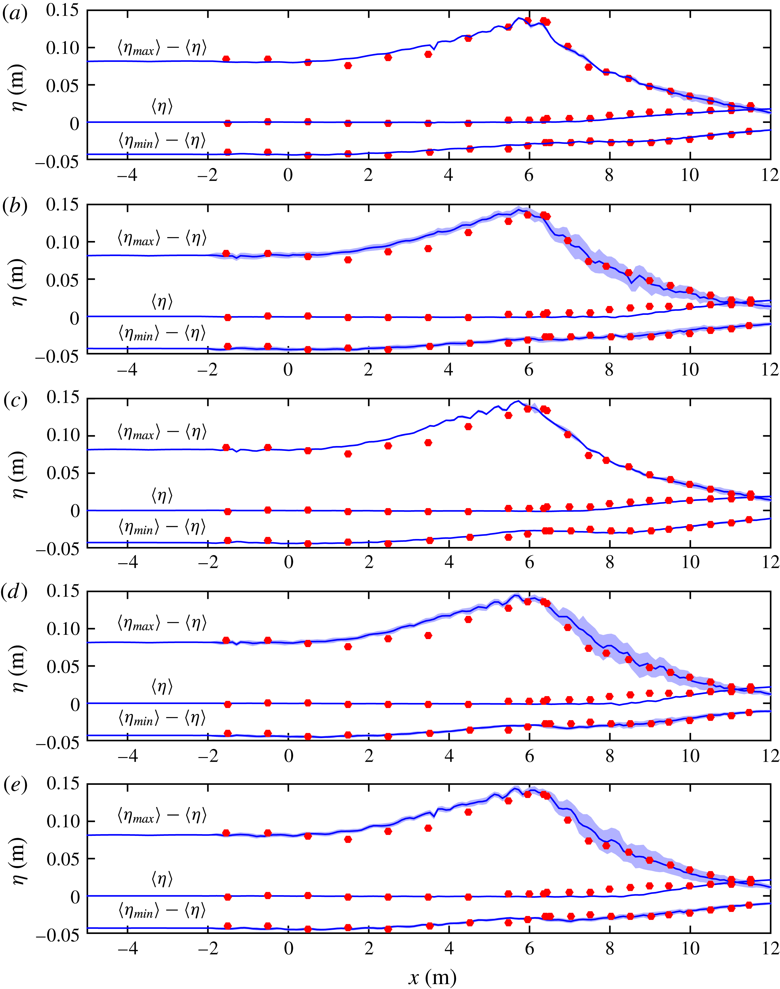
We will now further demonstrate the differences between results computed with standard (unstable) and new closure models via further quantitative comparison against the spilling breaker data set of Ting & Kirby (Reference Ting and Kirby1994). To make proper comparisons, as in the experiments, a relatively long warm up period is needed to establish stable conditions in the computational flume. Before extracting data, models have therefore been run for 60 periods. Such a long warm up period has not been common in most previous numerical studies of the Ting & Kirby (Reference Ting and Kirby1994) experiments. Jacobsen et al. (Reference Jacobsen, Fuhrman and Fredsøe2012) demonstrated, however, that at least 40 periods were necessary in order to reach a constant volume of water in their domain. We have similarly found that an additional 20 periods were necessary to achieve a convincing quasi-steady situation. For comparison, it can be noted that the warm up length in the experiments was 600 periods. Furthermore, in order to achieve stable mean values, the results presented in the following have been obtained by averaging over an additional 60 periods following the warm up (i.e. simulations have been run for a total of 120 periods). For comparison, in the original experiments the results were averaged over a comparable duration corresponding to 102 periods.

Figure 8.

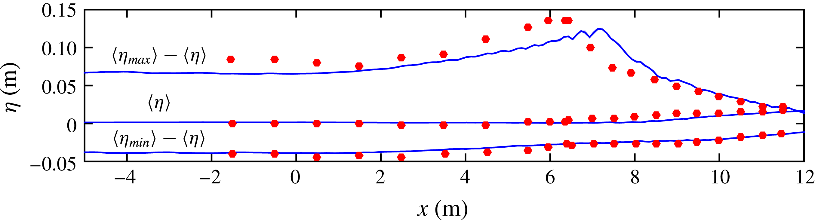
Comparison of modelled (lines) and measured (circles, from Ting & Kirby Reference Ting and Kirby1994) surface elevation envelopes (top and bottom lines) and mean water levels (middle lines). Results in (a–e) correspond to Cases 1–5, respectively. Solid lines represents the mean surface elevation and the shaded area represents plus and minus one standard deviation.

Figure 8 shows comparison of the computed and experimental surface elevation envelopes as well as the mean water levels for the five models mentioned above. The solid lines represent the mean (ensemble averaged) values, whereas the shaded area represents plus or minus one standard deviation, to give an indication of wave-to-wave variability. It can be seen that all five models, in general, capture the evolution of the mean surface elevations well. The horizontal position of the breaking point and surface elevation at breaking is well captured, as is the subsequent decay in wave heights in the surf zone. These results compare well with surface elevations presented in other numerical studies of these experiments, see e.g. Hieu et al. (Reference Hieu, Katsutohi and Ca2004), Jacobsen et al. (Reference Jacobsen, Fuhrman and Fredsøe2012), Xie (Reference Xie2013) and Brown et al. (Reference Brown, Greaves, Magar and Conley2016). The most notable difference between the models is the standard deviation in the surface elevations in the surf zone. As seen, those results sharing $\unicode[STIX]{x1D706}_{1}=0$ (i.e. the Wilcox (Reference Wilcox1988) model, Case 1 shown in figure 8(a) and our stabilized version of this model, Case 3 shown in figure 8 c) demonstrate little wave-to-wave variability. Conversely, the three results with the Wilcox (Reference Wilcox2006) limiter active ( $\unicode[STIX]{x1D706}_{1}>0$ , Cases 2, 4 and 5, respectively depicted in figure 8 b,d,e) result in significant wave-to-wave variability during the breaking process. Such variability is much more in line with the experiments (see e.g. figure 3 of Ting & Kirby Reference Ting and Kirby1994).

Figure 9.

Snapshots of the breaking process computed in (a) Case 3 ( $\unicode[STIX]{x1D706}_{1}=0$ , $\unicode[STIX]{x1D706}_{2}=0.05$ ) and (b) Case 4 ( $\unicode[STIX]{x1D706}_{1}=0.875$ , $\unicode[STIX]{x1D706}_{2}=0.05$ ), beginning at $t=t_{0}=110T$ . Here dark represents water, white represents air and light shades represent air–water mixtures. The wave shown in (a) never actually spills.

Further inspection has revealed that this lack in wave-to-wave variability computed with $\unicode[STIX]{x1D706}_{1}=0$ is due to the waves not breaking properly. This is due to large eddy viscosity computed in the crest (see figure 6 a,c), leading to turbulent dissipation of the wave rather than a convincing sequence of spilling breaking. This is illustrated in figure 9, where snapshots of typical waves computed during the breaking process are compared for Cases 3 ( $\unicode[STIX]{x1D706}_{1}=0$ ) and 4 ( $\unicode[STIX]{x1D706}_{1}=0.875$ ) i.e. two variants of the present stabilized model having different $\unicode[STIX]{x1D706}_{1}$ , but being otherwise identical. As a result of this failure of the waves to properly spill with $\unicode[STIX]{x1D706}_{1}=0$ , there is little deviation in the surface elevations experienced in successive waves in the surf zone. In contrast, the cases computed with $\unicode[STIX]{x1D706}_{1}>0$ , figure 8(b,d,e), spilling breaking occurs, leading to a much more dynamic surf zone. These results indicate that using a Wilcox (Reference Wilcox2006)-type limiter in the turbulent production is necessary to qualitatively capture the spilling breaking process. In the authors’ opinion, while at first glance the five results in figure 8 may appear similar, the inability of the $k$ – $\unicode[STIX]{x1D714}$ models with $\unicode[STIX]{x1D706}_{1}=0$ (figure 8 a,c corresponding to Cases 1 and 3) to predict proper spilling breakers (and corresponding wave-to-wave variability) can be regarded as an important qualitative shortcoming. We emphasize that the features discussed above (nature of breaking and subsequent wave-to-wave variability) are primarily dependent on the Wilcox (Reference Wilcox2006)-type limiter ( $\unicode[STIX]{x1D706}_{1}$ ), and have little to do with the new stabilizing limiter ( $\unicode[STIX]{x1D706}_{2}$ ) introduced in (2.35).

Figure 10.

Comparison of modelled (lines) and measured (circles) phase-averaged surface elevations at (a) $x=7.275$  m ( $\tilde{x}=(x-x_{b})/h_{b}=4.397$ ), (b) $x=7.885$  m ( $\tilde{x}=7.462$ ), (c) $x=8.495$  m ( $\tilde{x}=10.528$ ) and (d) $x=9.11$  m ( $\tilde{x}=13.618$ ).

To further illustrate the difference between cases with $\unicode[STIX]{x1D706}_{1}=0$ and $\unicode[STIX]{x1D706}_{1}>0$ , figure 10 shows a comparison between the experimental and computed phase-averaged surface elevations for Cases 3 and 5 at four different post-breaking cross-shore positions. In general the phase-averaged surface elevations match well for both cases, but there are two noteworthy features. First, in figure 10(a–c) the increase in surface elevation in Case 3 is more rapid than in Case 5. This can again be explained by the wave not properly breaking in Case 3 at these positions (as just shown in figure 9) resulting in a maintained steeper wave front. Second, in figure 10(d) Case 5 is significantly leading the experiments, indicating that the surface roller is apparently travelling too fast in the inner surf zone. The implications of this on the wave kinematics will be discussed later in this section.

Returning back to figure 8, considering the previous example from § 3.2, it may be somewhat surprising that the Wilcox (Reference Wilcox1988) and Wilcox (Reference Wilcox2006) models perform at all reasonably in terms of the mean surface elevations (figure 8 a,b). One might have expected that the large eddy viscosity would cause the waves to decay even prior to breaking, as was seen in the previous demonstration involving a propagating wave train (figure 4 a). This is, in fact, a real possibility, and the reason why this did not occur in the previous examples is merely due to the short propagation distance (in this case only a few wave lengths) allotted prior to the onset of breaking, which limits the extent of the turbulence over-production problem. Such pre-breaking wave decay would most certainly occur if the pre-slope distance was extended sufficiently further. To show this we have performed one additional simulation, but with the flat region now being 40 m instead of 4.7 m. The resulting surface elevations using the Wilcox (Reference Wilcox1988) model are shown in figure 11. Here it can be seen that the unstable growth in the eddy viscosity has caused the incoming wave to decline significantly, and as a consequence the horizontal position of the breaking point has shifted to be further onshore. Importantly, this recognition implies that previously computed results of breaking waves with non-stabilized closure models (prevalent in the literature) are not unique, instead being heavily dependent on both the initial conditions and the allotted propagation distance prior to shoaling and breaking. Results computed with the new stabilized closure, on the other hand, will be fundamentally insensitive to these issues.

Figure 11.

Comparison of computed (lines) and measured (Ting & Kirby Reference Ting and Kirby1994, circles) surface elevation envelopes and mean water levels using the Wilcox (Reference Wilcox1988) model with a long (40 m) flat region. This plot can be compared directly with figure 8(a), which depicts results computed with the same model, but where the flat region is only 4.7 m.

As further comparison, figure 12 presents computed and measured (Ting & Kirby Reference Ting and Kirby1994) averaged turbulent kinetic energy $k$ profiles at a total of eight positions, corresponding to two pre-breaking positions (figure 12 a,b), as well as six in the surf zone (figure 12 c–h). In the experiments only two components of the velocity were measured, so $k$ was approximated by $k\approx 1.33/2(\overline{u^{\prime 2}}+\overline{w^{\prime 2}})$ . This approximation was also used by Stive & Wind (Reference Stive and Wind1982) and Svendsen (Reference Svendsen1987), and comes from the results of a plane wake from Townsend (Reference Townsend1976). However more recent results from Scott et al. (Reference Scott, Cox, Maddux and Long2005) indicate that

(3.5) $$\begin{eqnarray}\displaystyle k\approx 0.75(\overline{u^{\prime 2}}+\overline{w^{\prime 2}}) & & \displaystyle\end{eqnarray}$$

in the surf zone, and this approximation has been used in what follows. Ting & Kirby (Reference Ting and Kirby1994) did not provide approximate $k$ -profiles in the two pre-breaking positions and the first post-breaking position (figure 12 a–c) as well as the top three measurement positions, but did provide profiles of the single component $\overline{u^{\prime 2}}$ . At these positions we have alternatively utilized the approximation

(3.6) $$\begin{eqnarray}\displaystyle k\approx 1.25\overline{u^{\prime 2}}, & & \displaystyle\end{eqnarray}$$

again based on the measurements of Scott et al. (Reference Scott, Cox, Maddux and Long2005). It is thus emphasized that the experimental $k$ -profiles must all be regarded as approximate, but are still likely reasonably indicative. For further discussions or indications on the uncertainties of such approximations see e.g. Ting & Kirby (Reference Ting and Kirby1996) and Scott et al. (Reference Scott, Cox, Maddux and Long2005).

Figure 12.

Comparison of modelled (lines) and measured (empty circles: from (3.5), filled circles: from (3.6)) turbulent kinetic energy $k$ profiles at (a) $x=-1.265$  m ( $\tilde{x}=(x-x_{b})/h_{b}=-38.518$ ), (b) $x=5.945$  m ( $\tilde{x}=-2.286$ ), (c) $x=6.665$  m ( $\tilde{x}=1.332$ ), (d) $x=7.275$  m ( $\tilde{x}=4.397$ ), (e) $x=7.885$  m ( $\tilde{x}=7.462$ ), (f) $x=8.495$  m ( $\tilde{x}=10.528$ ), (g) $x=9.11$  m ( $\tilde{x}=13.618$ ) and (h) $x=9.725$  m ( $\tilde{x}=16.709$ ).

To ease comparison the computed results in figure 12 are organized such that results with light shaded (blue) lines correspond to non-stabilized closures ( $\unicode[STIX]{x1D706}_{2}=0$ , Cases 1 and 2), whereas dark (black) lines correspond to formally stabilized models ( $\unicode[STIX]{x1D706}_{2}=0.05$ , Cases 3–5). Moreover, results having the same line type share common $\unicode[STIX]{x1D706}_{1}$ values, see again table 2. As might by now be expected, the standard Wilcox (Reference Wilcox1988) (Case 1) and Wilcox (Reference Wilcox2006) (Case 2) $k$ – $\unicode[STIX]{x1D714}$ models severely over-predict the turbulence pre-breaking (light shaded/blue lines in figure 12 a,b), which may again be regarded as a direct consequence of the instability of these models. The depicted over-production of turbulence using the Wilcox (Reference Wilcox1988) and Wilcox (Reference Wilcox2006) models is typical of previous studies. In contrast, the new stabilized closure models (Cases 3–5) predict low turbulent kinetic energy pre-breaking (dark black lines in figure 12 a,b, see also again figure 6), much more in line with the experiments. The improvement seen with the new stabilized closures in figure 12(a,b), and related effects further shoreward, can be regarded as the principal achievement of the present work: only waves computed with the new stabilized closure arrive at the surf zone, and hence begin the simulated breaking process, unpolluted. To most clearly see the isolated effect of the stabilizing limiter $\unicode[STIX]{x1D706}_{2}$ , Cases 1 and 2 can be respectively compared with Cases 3 and 4.

The over-production of turbulence prior to breaking using the non-stabilized models also has an effect on the post-breaking turbulence. As can be seen, both the Wilcox (Reference Wilcox1988) and Wilcox (Reference Wilcox2006) models (Cases 1 and 2) predict higher turbulence levels than their stabilized counterparts (respectively, Cases 3 and 4) during the initial breaking process (figure 12 c–e). This demonstrates that the unphysically high levels of pre-breaking turbulence predicted by the non-stabilized models can indeed pollute results extending well into the outer surf zone. Once the inner surf zone is reached (figure 12 f–h) the differences between the stabilized (dark black lines) and standard (light shaded/blue lines) turbulence models become smaller. Rather, the results in the inner surf zone are more governed by the value of the Wilcox (Reference Wilcox2006) stress limiter coefficient $\unicode[STIX]{x1D706}_{1}$ and have relatively little to do with $\unicode[STIX]{x1D706}_{2}$ . This can be clearly seen in figure 12, where the results having the same line type i.e. Cases 1 and 3 (dashed lines), and Cases 2 and 4 (dotted lines), which were initially quite different in figure 12(a–c), have become quite similar in figure 12(f–h). Thus, the stabilization of the closure models achieved by utilizing $\unicode[STIX]{x1D706}_{2}>0$ , as introduced herein, plays an important role both prior to breaking and in the outer surf zone, while expectedly becoming less important in the inner surf zone. This behaviour is as intended, as it has again been the aim of the present work to produce a formally stabilized closure model in potential flow regions, which defaults to a desired existing closure in sheared regions (i.e. the surf zone in the present context). The results in figure 12, as a whole, demonstrate that this has indeed been achieved.

Figure 13.

Comparison of modelled (lines) and measured (circles) undertow velocity profiles at (a) $x=-1.265$  m ( $\tilde{x}=(x-x_{b})/h_{b}=-38.518$ ), (b) $x=5.945$  m ( $\tilde{x}=-2.286$ ), (c) $x=6.665$  m ( $\tilde{x}=1.332$ ), (d) $x=7.275$  m ( $\tilde{x}=4.397$ ), (e) $x=7.885$  m ( $\tilde{x}=7.462$ ), (f) $x=8.495$  m ( $\tilde{x}=10.528$ ), (g) $x=9.11$  m ( $\tilde{x}=13.618$ ) and (h) $x=9.725$  m ( $\tilde{x}=16.709$ ).

To demonstrate the consequences directly on the flow properties, the computed and measured averaged undertow velocity profiles $\langle u(z)\rangle$ are finally compared in figure 13, at the same eight positions as in figure 12. Figure 13(a,b) clearly illustrates the adverse effects associated with the pre-breaking over-production of turbulence inherent within the standard Wilcox (Reference Wilcox1988) and Wilcox (Reference Wilcox2006) models (Cases 1 and 2, respectively). The negative peaks in the computed undertow with these models are consistently near the sea bed, whereas the measurements show these to be much higher up. This qualitative difference is important and can be explained by the artificially high $\unicode[STIX]{x1D708}_{T}$ in the upper part of the wave increasing the flow resistance, thus resulting in the strongest undertow near the bottom (similar to those profiles measured deeper into the surf zone). In contrast, in the experiments, as well as with the proposed new stabilized closure models (dark lines, Cases 3–5), the flow resistance is largest near the bed at these positions, and hence the undertow is strongest in the upper part of the flow.

The effects of over-produced turbulence in the outer surf zone are also clearly visible, with the two models having $\unicode[STIX]{x1D706}_{1}=0$ (Cases 1 and 3, dashed lines) maintaining an erroneous undertow structure (figure 13 c,d) while the cases with $\unicode[STIX]{x1D706}_{1}>0$ (Cases 2, 4 and 5) show a better evolution of the undertow structure at these positions. These results thus, again, highlight the positive influence of the Wilcox (Reference Wilcox2006) stress limiter, which was previously found essential to obtain properly spilling waves (figure 9). The model which best matches the evolution of the measured undertow structure from pre-breaking and throughout the outer surf zone (figure 13 a–e, corresponding to $-$ 1.265 m ${\leqslant}x\leqslant$ 7.885 m) is Case 5, corresponding to the present stabilized ( $\unicode[STIX]{x1D706}_{2}=0.05$ ) closure with the intermediate value $\unicode[STIX]{x1D706}_{1}=0.2$ . Notably, this transition from shoaling to the outer surf zone is a physically important and complex region of great interest, as the physics associated with the pre-to-post breaking transformation are related e.g. to the formation and dynamics of near-shore breaker bars, which play an important role in coastal protection.

Consistent with the trends seen previously in the computed turbulent kinetic energy, the results in the inner surf zone become grouped largely based on the value of $\unicode[STIX]{x1D706}_{1}$ utilized (figure 13 f–h) i.e. the results using (otherwise identical) formally stabilized or non-stabilized models are essentially similar in this region. The velocity profiles computed with $\unicode[STIX]{x1D706}_{1}>0$ (Cases 2, 4 and 5) remain qualitatively correct in structure, but become exaggerated by a factor of approximately two relative to those measured. It can be noted that very similar results for the undertow in the inner surf zone have been shown with various RANS closure models in Brown et al. (Reference Brown, Greaves, Magar and Conley2016), as well as with a LES model in Christensen (Reference Christensen2006). In contrast, the models using $\unicode[STIX]{x1D706}_{1}=0$ (Cases 1 and 3, dashed lines) actually result in more accurate undertow profiles in the inner surf zone. These results are certainly interesting, although in the authors’ opinion they should likely be regarded as fortuitous, given that these models did not result in (i) properly spilling waves or (ii) correct turbulence/undertow structure at many positions leading up to the inner surf i.e. a correct qualitative description of the breaking process is lacking with these models. (We again emphasize that the undertow in the inner surf zone is primarily dependent on the value of the Wilcox (Reference Wilcox2006)-type limiter $\unicode[STIX]{x1D706}_{1}$ , and has little to do with the new stabilizing $\unicode[STIX]{x1D706}_{2}$ -limiter introduced in (2.35).)

Upon further inspection of the present results, the quantitative differences in the undertow in the inner surf zone achieved with $\unicode[STIX]{x1D706}_{1}=0$ (Cases 1 and 3, dashed lines) and the other models are believed to be related to the waves computed with $\unicode[STIX]{x1D706}_{1}>0$ (Cases 2, 4 and 5) apparently travelling too fast once the inner surf zone is reached (see again figure 10 c). A surface roller travelling too fast, as is apparently the case with $\unicode[STIX]{x1D706}_{1}>0$ as exemplified with Case 5 in figure 10(c), will result in increased flow near the surface. This must be compensated by an increased undertow, hence promoting the exaggerations seen in figure 13(f–h) with $\unicode[STIX]{x1D706}_{1}>0$ .

The reason for the slower surface roller in Cases 1 and 3 (sharing $\unicode[STIX]{x1D706}_{1}=0$ ) relative to the other models is believed to be related to their increased eddy viscosity (hence flow resistance) in the upper part of the flow once in the inner surf zone. Such differences in the eddy viscosity are demonstrated in figure 14, where the average eddy viscosity profiles for Cases 3–5 at the two inner-most positions of the surf zone are shown. The higher eddy viscosity in Case 3 in the upper part of the flow extracts energy from the mean flow, slowing the breaking wave down compared to Case 5, as again shown in figure 10. Based on the locally improved undertow prediction, it seems that Case 3 apparently yields the ‘correct’ eddy viscosity in the inner surf zone. However, this model also clearly over-estimates $k$ in the upper part of the flow, as shown in figure 12(g,h) (seemingly a remnant of even more severe over-predictions further offshore). In the inner surf zone $\unicode[STIX]{x1D708}_{T}\approx k/\unicode[STIX]{x1D714}$ . The implication must then logically be that in Case 3 (similarly, Case 1) both $k$ and $\unicode[STIX]{x1D714}$ are locally erroneous, but by approximately the same factor, hence combining to produce an eddy viscosity that is more or less correct. In contrast, the models with $\unicode[STIX]{x1D706}_{1}>0$ (Cases 2, 4 and 5) yield quite reasonable $k$ -profiles in the inner surf zone (figure 12(g,h) implying that only $\unicode[STIX]{x1D714}$ is locally erroneous. How to obtain an accurate eddy viscosity in the upper part of flow in the inner surf zone, while still maintaining a proper description of the breaking process leading up to this region, remains an open question meriting further research.

Figure 14.

Comparison of modelled eddy viscosity profiles at (a) $x=9.11$  m ( $\tilde{x}=(x-x_{b})/h_{b}=13.618$ ) and (b) $x=9.725$  m ( $\tilde{x}=16.709$ ).

In summary, of utmost importance, the present case definitively demonstrates that the new stabilized closure proposed herein avoids entirely the important problem of non-physical over-production of turbulence prior to breaking, a long-standing problem in the CFD simulation of surface waves and the primary aim of the present paper. This, in turn, significantly improves both the prediction of turbulent kinetic energy and the evolution of the undertow as waves progress from the shoaling region to the outer surf zone. Conversely, due to their inherent instability, surface waves propagated with existing standard closure models can arrive at the surf zone already polluted, adversely affecting their results locally and extending into the outer surf zone. As intended, results with otherwise identical non-stabilized and stabilized closures become similar once the inner surf zone is reached. Of the five model variations tested, no single model has resulted in the best performance in all measured quantities at all positions, with the undertow in the inner surf zone proving the most elusive for the models which seem to give the best description leading up to this region. Nevertheless, having CFD models which begin the breaking process unpolluted by unphysical background turbulence is obviously important in studying the breaking process as a whole. Given that the instability addressed in the present work is inherent within the nearly potential flow region beneath waves, it is thus recommended that formally stabilized closure models, such as those presented herein, be utilized in future studies involving the RANS-based CFD study of surface waves.