


1. Introduction
Closed-loop control strategies such as linear optimal control (Anderson & Moore Reference Anderson and Moore1990) are commonly used in engineering and industrial applications, fluid dynamics being only one example of such. In the present paper we consider linear feedback control as a means to stabilise exact nonlinear solutions of the Navier–Stokes equations, or, exact coherent structures (ECS). The ECS have been instrumental in the explanation of the subcritical transition to turbulence. In many shear flows the transition to turbulence occurs despite the linear stability of the laminar profile. In pipe and plane Couette flow, for instance, the laminar profile is linearly stable at all Reynolds numbers. Plane Poiseuille flow becomes linearly unstable at a Reynolds number of  $5772.22$ (Orszag Reference Orszag1971a); however, when subjected to finite-amplitude perturbations the flow transitions much earlier. Exact coherent structures and their stability properties are not only of interest to studies concerned with transitional flows. There is ample evidence supporting the concept whereby the turbulent region of the state space of a wall-bounded, parallel shear flow includes many unstable ECS (Nagata Reference Nagata1990; Hof et al. Reference Hof, van Doorne, Westerweel, Nieuwstadt, Faisst, Eckhardt, Wedin, Kerswell and Waleffe2004, Reference Hof, van Doorne, Westerweel and Nieuwstadt2005; Eckhardt et al. Reference Eckhardt, Schneider, Hof and Westerweel2007; Duguet, Pringle & Kerswell Reference Duguet, Pringle and Kerswell2008a; Duguet, Willis & Kerswell Reference Duguet, Willis and Kerswell2008b; Kawahara, Uhlmann & van Veen Reference Kawahara, Uhlmann and van Veen2012; Cvitanović Reference Cvitanović2013; Willis, Short & Cvitanović Reference Willis, Short and Cvitanović2016; Budanur et al. Reference Budanur, Short, Farazmand, Willis and Cvitanović2017; Suri et al. Reference Suri, Tithof, Grigoriev and Schatz2017; Reetz, Kreilos & Schneider Reference Reetz, Kreilos and Schneider2019; Reetz & Schneider Reference Reetz and Schneider2020; Reetz, Subramanian & Schneider Reference Reetz, Subramanian and Schneider2020), with turbulence corresponding to a state-space trajectory travelling along the ECS’ stable and unstable manifolds resulting in frequent close passes to different ECS. Once the state-space trajectory is in close vicinity of an ECS, the properties of the turbulent state approximate those of that ECS. Exact solutions of the Navier–Stokes equations can differ considerably in their global and local properties, such as drag, mean profile or turbulence intensity. The application of a feedback control procedure can be a useful strategy to avoid states with undesirable properties such as high drag by altering their stability properties, thus preventing state-space trajectories from remaining close to certain ECS or confining the dynamics to certain state-space volumes. A dynamic feedback procedure based on adjustments of the Richardson number succeeded in temporal stabilisation of otherwise transient turbulent spots and stripes in stratified plane Couette flow (Taylor etal. Reference Taylor, Deusebio, Caulfield and Kerswell2016).
A further potential application for feedback control in the context of ECS lies in the determination of so-called edge states, relative attractors on the edge of chaos, a codimension-1 manifold in state space that distinguishes between initial conditions resulting in laminar or turbulent flow. The concept of edge states and edge manifolds is intrinsically connected to the transition to turbulence in many wall-bounded shear flows such as pipe, plane Couette and channel flows (Itano & Toh Reference Itano and Toh2001; Skufca, Yorke & Eckhardt Reference Skufca, Yorke and Eckhardt2006; Eckhardt et al. Reference Eckhardt, Schneider, Hof and Westerweel2007). Depending on the extent of the domain, edge states may be invariant solutions of the Navier–Stokes equations or have chaotic dynamics and contain invariant solutions (Budanur & Hof Reference Budanur and Hof2018). Edge states, or the invariant solutions contained therein, have by definition one unstable direction transverse to the edge (Schneider, Eckhardt & Yorke Reference Schneider, Eckhardt and Yorke2007; Duguet et al. Reference Duguet, Willis and Kerswell2008b), such that the dynamics will not remain confined to it. The latter makes the determination of edge states, or invariant solutions therein, difficult. Bisection-based numerical methods (Itano & Toh Reference Itano and Toh2001; Skufca et al. Reference Skufca, Yorke and Eckhardt2006; Schneider et al. Reference Schneider, Eckhardt and Yorke2007) are available, but they are costly due to slow convergence and high computational effort. Edge states can also be probed by minimal seed methods (Pringle & Kerswell Reference Pringle and Kerswell2010; Pringle, Willis & Kerswell Reference Pringle, Willis and Kerswell2012, Reference Pringle, Willis and Kerswell2015), as the smallest perturbation triggering turbulence, the minimal seed, is located infinitesimally close to the edge. It evolves along the edge, passes close to the edge state and eventually enters the turbulent region of state space.
In small simulation domains or in symmetry-invariant subspaces edge states are part of an unstable lower branch of ECS that appear in a saddle-node bifurcation. In large domains, when edge states are chaotic and can contain ECS (Budanur & Hof Reference Budanur and Hof2018), lower-branch ECS can be found within the edge state. This suggests that low-dimensional feedback stabilisation methods could be used to remove the effect of the unstable directions, such that the edge state, or an invariant solution therein, is stabilised. In pipe flow, a simple feedback control strategy, where the Reynolds number is adjusted in response to an observable connected with deviations from laminar flow, indeed stabilises the dynamics to remain on the edge (Willis et al. Reference Willis, Duguet, Omel'chenko and Wolfrum2017). Forward integration of the controlled system converged to previously unknown edge states in the form of travelling waves. For more complicated edge states, such as relative periodic orbits or those with chaotic dynamics, the controlled simulations converged to objects in the vicinity of ECS of the uncontrolled system.
Here, we focus on feedback strategies in channel flow at Reynolds numbers below the linear stability threshold, as an example system showing a subcritical transition to turbulence. In order to highlight and discuss the challenges that arise in the application of linear feedback control for the stabilisation of exact coherent structures, we attempt to stabilise some of simplest invariant solutions in minimal flow units, that is, edge states in form of travelling waves. Unlike Willis et al. (Reference Willis, Duguet, Omel'chenko and Wolfrum2017) we aim to stabilise known invariant solutions. To do so, we construct simple linear feedback procedures that are either (i) pressure based and thus one step closer to experimental conditions, or (ii) adjoint based and act on the single unstable direction by construction. In the first case, we monitor the controller's effect on global observables such as turbulent kinetic energy and skin friction coefficient, and we find that the controlled dynamics approaches values of these observables that correspond to the target states; however, the target states themselves are not stabilised. The reason lies in the occurrence of a new instability that is induced by the coupling of the control procedure to the edge states’ stable directions. The second method removes such secondary instabilities by construction; however, care must be taken in its application in terms of the type of target state and the choice of global observable. Here, only a highly symmetric de-localised travelling wave has been successfully stabilised with this method, which illustrates the limitations of global 1-D feedback.
We begin with an introduction to the concept of linear feedback control in § 2 in the context of invariant solutions, where the procedure is explained and its effect is illustrated in low-dimensional examples. In § 3 we use the general formalism outlined in § 2 to develop the control strategies. Before applying the control procedures to the aforementioned edge states in direct numerical simulations of channel flow, we summarise the numerical details and describe the target states in § 4. Section 5 contains the main investigation into stabilisation of edge states including the effect of the feedback control on the stable directions. We summarise our results in § 6 alongside a discussion of the challenges that need to be overcome in the design of successful control strategies in the context of simple invariant solutions of the Navier–Stokes equations.
2. Stabilisation and control
Consider a system with two variables, a positive observable  $A$ and a control variable
 $R$. In fluid dynamics,
 $A$ could be the result of a global measurement such as the skin friction factor or a local measurement such as the magnitude of the turbulent fluctuations, and
 $R$ the Reynolds number, which is here interpreted as a means to determine the pressure gradient as the control input. We assume that the uncontrolled system has stationary solutions that appear in a saddle-node bifurcation at
 $(A^*, R^*)$ with an unstable lower branch
 $A_{LB}(R)$. The aim is to stabilise an operating point
 $(A_0,R_0)$ on the lower branch (Sieber, Omel'chenko & Wolfrum Reference Sieber, Omel'chenko and Wolfrum2014; Willis et al. Reference Willis, Duguet, Omel'chenko and Wolfrum2017). Without loss of generality we further assume that the uncontrolled dynamics is such that the observable grows if it exceeds the lower-branch value
 $A_{LB}(R)$,
 \begin{equation} \dot{A} = \lambda (A-A_{LB}(R)), \end{equation}
with  $\lambda > 0$ being the Lyapunov exponent, which we assume to be independent, or a slowly varying function, of
 $R$. To control and avoid the exponential instability, the control variable must be repeatedly adjusted such that the ensuing dynamics of the system results in convergence to the operating point, for example through an iteration procedure where the lower branch is crossed at each adjustment of the control variable as schematically illustrated in figure 1. For the uncontrolled dynamics as in (2.1), this can be achieved by adjusting the control variable according to
 \begin{equation} \dot{R} ={-} \gamma \left(R - R_0\right) - \gamma \mu (A-A_0), \end{equation}
where  $A_0=A(R_0)=A_{LB}(R_0)$ is the value of the observable at the reference point and
 $\gamma > 0$ and
 $\mu > 0$ are adjustable parameters. The signs are for the cases that
 $A_{LB}(R)$ decreases with
 $R$, i.e.
 \begin{equation} \left. \frac{\textrm{d} A_{LB}(R)}{\textrm{d}R} \right|_{R_0} ={-} \alpha, \end{equation}
with  $\alpha >0$. With
 $r=R-R_0$ and
 $a = A-A_0$ we can write
 \begin{equation} A- A_{LB}(R) = A - A_{LB}(R_0+r) \approx a + \alpha r, \end{equation}
so that (2.1) and (2.2) become
 \begin{equation} \frac{\textrm{d}}{\textrm{d}t} \begin{pmatrix} a \\ r \end{pmatrix} = \begin{pmatrix} \lambda & \lambda \alpha \\ - \gamma \mu & - \gamma \end{pmatrix} \begin{pmatrix} a \\ r \end{pmatrix} . \end{equation}
For the operating point  $(A_0,R_0)$ to be stable, the matrix on the right-hand side of (2.5) must have eigenvalues with negative real parts. The conditions for such eigenvalues are that the trace of the matrix, as the sum of the eigenvalues, has to be negative, and the determinant, the product of the eigenvalues, has to be positive. With the trace
 \begin{equation} \text{Tr}= \lambda - \gamma, \end{equation}
and the determinant
 \begin{equation} \text{det}={-} \lambda \gamma + \lambda \gamma \alpha \mu, \end{equation}
the conditions for stability become
 \begin{gather} \gamma > \lambda, \end{gather}
 \begin{gather} \alpha\mu > 1 . \end{gather}
The conditions are such that the adjustment in  $R$ (related to the parameter
 $\gamma$) has to be faster than the escape (as measured by
 $\lambda$). Similarly, the amplitude of the change in the control variable with the deviation in the observable has to be larger than the inverse of
 $\alpha$, so that the changes in
 $R$ outrun the changes in
 $A$. For what follows it will be useful to visualise the stability condition (2.9) geometrically: since
 $\alpha$ is the slope of the tangent to the lower branch at
 $(A_0,R_0)$, the inequality (2.9) results in a control line through
 $(A_0,R_0)$ with a slope
 $1/\mu < \alpha$ which is shallower than that of the tangent at the operating point. The feedback control procedure applied by Willis et al. (Reference Willis, Duguet, Omel'chenko and Wolfrum2017) corresponds in this context to an immediate adjustment of
 $R$, i.e. to
 $\gamma \to \infty$.
Schematic dynamics of the controlled system. The unstable lower branch (dashed line) is curved towards smaller values of the observable for increasing control variable. The red (grey) dot on the lower branch corresponds to an operating point. For an initial state below the lower branch indicated by the light green (light grey) dot, the uncontrolled dynamics is such that the value of the observable decreases, resulting in intermediate states further below the lower branch as indicated by the green (dark grey) dot. The feedback control increases the control variable until the lower branch is crossed, such that the uncontrolled dynamics now results in a growing observable. The feedback control now decreases the value of the control variable until the lower branch is crossed again to enter the region where the observable will decay. Iteration of this procedure will eventually result in convergence towards the operating point.

Before proceeding to numerical results, we briefly highlight the connection between the present formulation of the linear control law given in (2.5) and linear feedback control. If we combine the observable  $a$ and the control variable
 $r$ into one state vector
 $\boldsymbol {x}$, then the uncontrolled linearised dynamics, where
 $r = 0$ and
 $\dot {r} = 0$, is given by
 \begin{equation} \underbrace{\begin{pmatrix} \dot{a} \\ \dot{r} \end{pmatrix}}_{\dot{\boldsymbol{x}}} = \underbrace{\begin{pmatrix} \lambda & 0 \\ 0 & 0 \end{pmatrix}}_{\mathcal{A}} \underbrace{\begin{pmatrix} a \\ r \end{pmatrix}}_{\boldsymbol{x}}, \end{equation}
with Jacobian  $\mathcal {A}$. The control law given in (2.2) makes
 $r$ time dependent such that (2.5) can be written in classical control-theoretic form as closed-loop feedback control
 \begin{equation} \dot{\boldsymbol{x}} = \mathcal{A} {\boldsymbol{x}} - \mathcal{BK} {\boldsymbol{x}}, \end{equation}
where  $\mathcal {B}$ is the control matrix and, for stabilisation according to linear optimal control or full state feedback, the matrix
 $\mathcal {K}$ must be chosen such that
 \[ \mathcal{A} - \mathcal{BK} = \begin{pmatrix} \lambda & \lambda \alpha \\ - \gamma \mu & - \gamma \end{pmatrix} \]
has only eigenvalues with negative real part, see e.g. Anderson & Moore (Reference Anderson and Moore1990), Sontag (Reference Sontag1998) and Burl (Reference Burl1999).
2.1. Two-dimensional linear model
Before applying the feedback control to a high-dimensional dynamical system such as channel flow, we consider the dynamics of the linearised two-dimensional (2-D) system given by (2.5), with Lyapunov exponent  $\lambda = 0.01$, and lower-branch slope
 $\alpha = 1.5 \times 10^{-5}$. These values correspond to measurements of
 $\alpha$ and
 $\lambda$ for an edge state in direct numerical simulations of channel flow, which will be discussed in further detail in § 4. Figure 2 presents phase-space trajectories of this system for
 $\gamma = 1$ and two different values of the control strength
 $\mu$, i.e.
 $\mu = 2 \times 10^5$ and
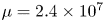 $\mu = 2.4 \times 10^7$. The tangent line as indicated in orange (light grey) has a steeper slope than the control line (blue/dark grey) in both cases, as required by (2.9), and both lines cross at the operating point. The time evolution follows the green/grey curve, beginning at the red/grey points located in the top right quadrants of the two panels, and it ends at the operating point. That is, in both cases the operating point has been stabilised.
Stabilisation of the linear model system given by (2.5). The (linear) lower branch is indicated by the dashed line, it crosses the control line (solid black) at the operating point. The time evolution of the system follows the red (grey) curve starting at the blue (dark grey) square. ( $a$) Monotonic relaxation for
 $\mu = 2 \times 10^5$ corresponding to negative real eigenvalues. (
 $b$) Oscillatory relaxation for
 $\mu = 2.4 \times 10^7$ corresponding to complex eigenvalues with negative real parts.

In both cases the instability has been removed, leading to eigenvalues of the matrix in (2.5) that have negative real parts. The eigenvalues do not only yield information on the stability of an equilibrium in the controlled system, they also determine the dynamic relaxation process. For real eigenvalues we expect monotonic exponential relaxation, while complex eigenvalues with non-zero imaginary part lead to an oscillatory approach to the stabilised equilibrium. In the present linear 2-D model system, the eigenvalues are real for  $\mu = 2 \times 10^5$ and complex for
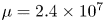 $\mu = 2.4 \times 10^7$, and the relaxation towards the equilibrium does indeed proceed differently for the two values of the control strength. For
 $\mu = 2 \times 10^5$ the relaxation proceeds monotonically along the control line as shown in figure 2(a), while
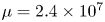 $\mu = 2.4 \times 10^7$ results in oscillatory relaxation as shown in figure 2(b). The latter is reminiscent of the schematic behaviour illustrated in figure 1.
2.2. Effect on the stable directions
Equilibria in higher-dimensional systems can have several stable and unstable directions. Even if we assume that only one direction is unstable, as is generally the case for edge states in canonical wall-bounded parallel shear flows, a 1-D control procedure may not only have the desired influence on the unstable direction, it may also couple to the stable directions. This effect is known in control theory, where its mitigation is essential in the design of successful controllers (Barbagallo, Sipp & Schmid Reference Barbagallo, Sipp and Schmid2009). In order to illustrate what the consequences of such a coupling can be, we consider a three-dimensional (3-D) extension of the 2-D model given in linearised form in (2.5):
 \begin{equation}
\frac{\textrm{d}}{\textrm{d}t} \left( \begin{matrix} r \\
a_1 \\ a_2 \end{matrix} \right) = \left(
\begin{matrix} - \gamma & - \gamma \mu_1 & -\gamma \mu_2 \\
\lambda_1 \alpha_1 & \lambda_1 & 0 \\ -\lambda_2 \alpha_2 &
0 & -\lambda_2 \end{matrix} \right) \left( \begin{matrix} r
\\ a_1 \\ a_2 \end{matrix} \right),
\end{equation}
where  $a_1$ corresponds to the unstable and
 $a_2$ to the stable direction with
 $\lambda _1 > 0$ and
 $\lambda _2 > 0$. The dynamics is coupled to the control procedure through
 $\mu _1$ and
 $\mu _2$, respectively. For simplicity, we assume that the stable and unstable directions decouple. For
 $a_1 = a$,
 $\lambda _1 = \lambda$ and
 $\alpha _1 = \alpha$ as in figure 2, we construct arbitrary stable directions by randomly choosing
 $a_2 > 0$,
 $\lambda _2 > 0$ and
 $\alpha _2 > 0$ to avoid a specific configuration. Subsequently and for fixed values of
 $a_2 > 0$,
 $\lambda _2 > 0$ and
 $\alpha _2 > 0$, we calculate the number of eigenvalues of the matrix on the right-hand side of (2.12) that have a positive real part as a function of
 $\mu _1$ and
 $\mu _2$. An example of the results obtained from such a calculation is shown in figure 3. If the control is weakly coupled to the dynamical system, we find one eigenvalue with positive real part, as expected for a system with one stable and one unstable direction. Increasing
 $\mu _1$ for small
 $\mu _2$ eventually stabilises the operating point, which can also be expected from the results in the 1-D case. However, we find a large part of parameter space where one or two eigenvalues have a positive real part, hence the control is not able to stabilise the operating point if it overlaps significantly with the stable direction.
Destabilisation of a stable direction for the 3-D model system given by (2.12). The colour coding represents the number of eigenvalues of the matrix on the right-hand side of (2.12) that have positive real parts. The coupling of the control to the unstable and stable directions is parametrised by  $\mu _1$ and
 $\mu _2$, respectively.

In summary, the success of the control strategy in higher-dimensional systems depends on how the dynamics along the stable directions couples to the control. Stabilisation of the operating point then requires a control strategy that acts on a hyperplane orthogonal to all stable directions. Such a strategy can be constructed in numerical simulations only, and we will come back to this point in § 5.2. In practice, the control is more likely to destabilise stable directions with a small negative real part, which suggests that it may be sufficient to design the control to be orthogonal to the least stable directions in order to achieve stabilisation. Similar procedures are indeed sometimes applied in control theory in the context of model reduction (Åkervik et al. Reference Åkervik, Hœpffner, Ehrenstein and Henningson2007) and will be successful provided the chosen modes are observable and controllable (Barbagallo et al. Reference Barbagallo, Sipp and Schmid2009).
3. Linear feedback control for the Navier–Stokes equations
Having introduced a general 1-D feedback control strategy and discussed its properties in low-dimensional model systems, we now turn to its application to wall-bounded shear flows, whose dynamics is governed by the incompressible Navier–Stokes equations
 \begin{gather} \partial_t \boldsymbol{u} + \boldsymbol{u} \boldsymbol{\cdot} \boldsymbol{\nabla} \boldsymbol{u} ={-}\boldsymbol{\nabla} p + \nu{\rm \Delta} \boldsymbol{u} + \frac{1}{\rho}\boldsymbol{f}, \end{gather}
 \begin{gather} \boldsymbol{\nabla} \boldsymbol{\cdot} \boldsymbol{u} = 0, \end{gather}
where  $\boldsymbol {u}$ is the velocity field,
 $p$ the pressure divided by the constant density
 $\rho$,
 $\nu$ the kinematic viscosity and
 $\boldsymbol {f}$ a force that drives the flow. The implementation of the feedback procedure introduced in § 2 requires a choice of observable and control variable. Here, care must be taken in the non-dimensionalisation of (3.1), as the choice of control variable may result in the usual characteristic scales becoming time dependent. Furthermore, (3.1) must be supplemented with an auxiliary equation that describes the time evolution of the control variable as a function of the observable. The feedback loop is then closed by coupling the control variable to (3.1).
In principle, there are two conceptual choices for the control variable, one that results in a modulation of the flow and one that results in an adjustment of  $\boldsymbol {f}$. Since (3.1) is usually made dimensionless using a characteristic length scale
 $h$ and a reference velocity
 $U_0$, the choice of control variable must be such that
 $U_0$ and
 $h$ remain time independent. Otherwise the dimensionless form of (3.1) is not applicable any longer because the time derivative does not commute with the now time-dependent reference velocity
 $U_0(t)$. This occurs if the feedback is implemented through a modulation of the flow. Therefore, we focus here on the second possibility, that of an adjustment of
 $\boldsymbol {f}$ in response to a control variable. Assuming that
 $\boldsymbol {f}(t)$ fluctuates around a reference state
 $\boldsymbol {f}_0$, the velocity scale
 $U_0$ that is associated with that particular value of the force is used to rescale (3.1). Specifically, the forcing is made dimensionless in units of
 $h/U_0^2$, and variations in the force can be measured in the same units. In what follows,
 $U_0$ is the laminar centreline velocity and
 $h$ the half-height of the channel.
3.1. A pressure-based control strategy
For pressure-driven pipe or channel flow, the control input  $\boldsymbol {f}$ can be identified with a time-dependent streamwise pressure gradient
 $\textrm {d}P/\textrm {d}x(t)\boldsymbol {e}_x$ that fluctuates around a reference value
 $(\textrm {d}P/\textrm {d}x)_0 \boldsymbol {e}_x$. The controlled system in non-dimensionalised form then reads
 \begin{gather} \partial_t \boldsymbol{u} + \boldsymbol{u} \boldsymbol{\cdot} \boldsymbol{\nabla} \boldsymbol{u} +\boldsymbol{\nabla} p - \frac{1}{Re}{\rm \Delta} \boldsymbol{u} + \left(\frac{\textrm{d}P}{\textrm{d}x}\right)_0 \boldsymbol{e}_x ={-}\frac{\textrm{d}P}{\textrm{d}x}(t)\boldsymbol{e}_x, \end{gather}
 \begin{gather} \boldsymbol{\nabla} \boldsymbol{\cdot} \boldsymbol{u} = 0, \end{gather}
 \begin{gather} \dot{R} ={-} \gamma \left(R - R_0\right) - \gamma \mu (A-A_0), \end{gather}
 \begin{gather} \frac{\textrm{d}P}{\textrm{d}x}(t) ={-}\frac{2}{R_0}\left(\frac{R(t)}{R_0}-1\right), \end{gather}
with  $A$ being an observable,
 $R$ the control variable with
 $(R_0, A_0)$ defining the operating point. Equation (3.6), which implements the feedback, is based on
 $R$ representing a Reynolds number such that
 $R = R_0 = Re$ results in no control input and the reference pressure gradient is recovered. The time-dependent Reynolds number that is used by Willis et al. (Reference Willis, Duguet, Omel'chenko and Wolfrum2017) cannot be realised with a change in the pressure gradient or similar, since that would give a different velocity scale, as discussed above. As it stands, a modulation in Reynolds number can only be obtained as a consequence of variations in viscosity, which is difficult to achieve in experiments.
In order to stabilise the operating point, the control must overlap with the expanding directions of the operating point's tangent space. Since the linear operator representing the linearised Navier–Stokes dynamics close to the operating point is non-normal, its eigenvectors are not orthogonal. That is, it is in principle possible to stabilise an operating point with a 1-D control procedure, provided that all unstable directions overlap. Here, the proposed feedback control acts in the streamwise direction only and it is translationally invariant in both streamwise and spanwise directions. That is, it can only stabilise unstable directions that have a streamwise component with a non-zero streamwise and spanwise mean. Periodic instabilities, for instance, cannot be stabilised. This is an example of a more general effect that symmetries, translational invariance being an example thereof, have on controllability and observability in linear feedback control (Grigoriev Reference Grigoriev2000). Formally speaking, an  $n$-dimensional system is controllable if the vectors
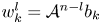 $w_k^l = \mathcal {A}^{n-l}b_k$ for
 $1 \leq k \leq n$ and
 $1 \leq l \leq m$, where
 $\mathcal {A}$ is the Jacobian governing the linearised dynamics and
 $b_k$ denotes the
 $k$th column vector of the control matrix
 $\mathcal {B} = (b_1, \ldots, b_m)$, form a basis of the tangent space at the operating point. An equivalent formulation is that each eigenmode must have non-zero overlap with at least one column vector of
 $\mathcal {B}$. Symmetries may lead to eigenspaces of the linear operator
 $\mathcal {A}$ of dimension larger than one, and hence basis vectors of such eigenspaces exist which are orthogonal to all
 $b_k$ (Grigoriev & Cross Reference Grigoriev and Cross1998; Grigoriev Reference Grigoriev2000). Similar issues also concern, in principle, the question of observability; however, such complications do not arise in the present context as we have access to the full state of the system at any point in time.
3.2. Adjoint-based control
The potentially destabilising effect of the control given by (3.3)–(3.6) calls for a strategy that acts on the unstable direction only. In what follows we construct a control that acts on a hyperplane orthogonal to the stable subspace of the ECS's tangent space and hence cannot couple and destabilise the contracting directions. Similar approaches are used in controlling linear, infinite-horizon problems. There, the optimal control strategy is of feedback type and proceeds by projection of the state vector onto its unstable eigenspace and an appropriate choice of coupling coefficients such that the linear operator representing the controlled system has only stable eigenmodes (Anderson & Moore Reference Anderson and Moore1990; Burl Reference Burl1999).
We consider a general  $n$-dimensional dynamical system
 \begin{equation} \dot{\xi} = F(\xi), \end{equation}
where  $F$ is a differentiable function that governs the time evolution of
 $\xi$. In the present application
 $\xi$ represents the Galerkin-truncated velocity field and
 $F$ the time evolution given by the appropriately truncated version of (3.1) in terms of a finite number of coupled ordinary differential equations. Let
 $\xi _0$ correspond to the operating point, then the linearised dynamics close to
 $\xi _0$ are given by
 \begin{equation} \dot{\delta} \xi = J_F\delta \xi, \end{equation}
where  $J_F=J_F(\xi _0)$ is the Jacobian of
 $F$ at
 $\xi _0$. The tangent space at
 $\xi _0$ is then spanned by the right eigenvectors
 $\{v_i\}_{(i = 1, \ldots, n)}$ of
 $J_F$. Since
 $J_F$ is in general non-normal, the
 $\{v_i\}$ are not mutually orthogonal, i.e.
 $(v_i,v_j) \neq \delta _{ij}$, with
 $(\cdot, \cdot )$ being an inner product on the tangent space at
 $\xi _0$. Hence, a control procedure that overlaps with the unstable directions may also overlap with the stable and the marginal ones. However, the dual basis
 $\{v_i^*\}$, defined as the set of linear maps from the tangent space at
 $\xi _0$ to
 $\mathbb {C}$ satisfying
 $v_i^*(v_j) = \delta _{ij}$ satisfies the desired bi-orthogonality constraints by definition
 $(v_i,v_j^*) := v_i^*(v_j) = \delta _{ij}$. If we have
 $k<n$ unstable directions,
 $v_1,\ldots,v_k$, a control that is constructed as a linear combination of the duals
 $v_1^*,\ldots,v_k^*$ will be orthogonal to all stable and marginal directions. More specifically, the purpose of a feedback control with control input
 $f(\xi )$ is to stabilise
 $\xi _0$, that is, to ensure that all eigenvalues of
 $J_{F} + J_f$, where
 $J_f=J_f(\xi _0)$ is the Jacobian of
 $f$ at
 $\xi _0$, have negative or zero real parts. For reasons of clarity and conciseness, we assume from now on that
 $J_{F}$ has one expanding direction
 $v_e$, as the generalisation to more unstable directions is straightforward. If we construct
 $f$ to act along
 $v_e^*$ such that the controlled dynamical system is given by
 \begin{equation} \dot{\xi} = F(\xi) + f(\xi) = F(\xi) + \kappa(\xi)v_e^*, \end{equation}
where  $\kappa$ is a function of
 $\xi$ implementing the feedback, then the controlled linearised system is
 \begin{equation} \dot{\delta} \xi = \left(J_F + J_f \right)\delta \xi = \left(J_F + v_e \otimes \boldsymbol{\nabla}\kappa \right)\delta \xi, \end{equation}
where  $\boldsymbol {\nabla } \kappa$ denotes the gradient of
 $\kappa$ at
 $\xi _0$ and we use tensor product notation for
 $J_f$, that is
 $(a \otimes b)_{ij} := a_i b_j$ for two generic vectors
 $a$ and
 $b$. Since the dimension of the tangent space at any point equals that of the underlying manifold, we can expand
 $\delta \xi$ at any point in time in terms of the basis
 $v_i$
 \begin{equation} \delta \xi(t) = \sum_i a_i(t)v_i, \end{equation}
where  $a_i$ are time-dependent coefficients. Equation (3.10) becomes
 \begin{align} \sum_i \dot{a}_i(t)v_i & = \left(J_F + v_e \otimes \boldsymbol{\nabla}\kappa \right) \sum_i a_i(t)v_i = \sum_{i} \left(\lambda_i+ \sum_jk_j v_e \otimes v_j \right)a_i(t)v_i \nonumber\\ & = \sum_{i} \lambda_i a_i(t)v_i + \sum_{i,j}a_i(t)k_j (v_j^*, v_i) v_e \nonumber\\ & = \sum_{i} \lambda_i a_i(t)v_i + \sum_{i,j}a_i(t)k_j \delta_{ij} v_e \nonumber\\ & = \sum_{i \neq e} \lambda_i a_i(t)v_i + \left(\lambda_e a_e(t)+ \left(\sum_i k_i a_i(t) \right) \right)v_e, \end{align}
where  $\lambda _i$ are the eigenvalues of
 $J_F$ and
 $k_j = (\boldsymbol {\nabla } \kappa ^*, v_j)$. By taking the inner product of both sides of this equation with
 $v_e^*$ it can be seen that
 $\xi _0$ is stabilised if
 $k_i = 0$ for
 $i \neq e$ and if
 \begin{equation} \lambda_e + k_e \leq 0, \end{equation}
that is, the gradient of the feedback function  $\kappa$ at the operating point must be colinear with the unstable direction. In the present example of channel flow, the control input
 $\kappa$ is determined by the choice of observable. An observable that is quadratic in the velocity field will result in
 $\boldsymbol {\nabla } \kappa$ being colinear with the operating point. If the latter then has a significant overlap with the unstable direction, the choice of observable may work well. Close inspection of the unstable direction can yield further information, for example if the instability is mostly in span- or wall-normal directions, the cross-flow energy is a good observable.
For time-independent operating points, i.e. equilibria of (3.7), with one unstable eigenmode, the implementation of such a control procedure results in replacing the unit vector  $\boldsymbol {e}_x$ on the right-hand side of (3.3) with the dual of the solution'sunstable eigenmode,
 $v^*_e$, which has been normalised to be a unit vector. The generalisation to more unstable directions is straightforward. For travelling-wave or periodic solutions, the implementation is slightly more complicated as the time dependence of the target state has to be accounted for. For a wave travelling in the streamwise direction with speed
 $c$ the adjoint-based control strategy is given by (3.4)–(3.5), with (3.3) replaced by
 \begin{equation} \partial_t \boldsymbol{u} + \boldsymbol{u} \boldsymbol{\cdot} \boldsymbol{\nabla} \boldsymbol{u} +\boldsymbol{\nabla} p - \frac{1}{Re}{\rm \Delta} \boldsymbol{u} + \left(\frac{\textrm{d}P}{\textrm{d}x}\right)_0 \boldsymbol{e}_x = \frac{2}{R_0}\left(\frac{R(t)}{R_0}-1\right)\sigma_c(t)(v^*_e), \end{equation}
where  $\sigma _c$ is the shift operator in the streamwise direction
 \begin{equation} \sigma_c(t): \boldsymbol{u}(x,y,z) \mapsto \boldsymbol{u}(x+ct,y,z) . \end{equation}
Shifts in spanwise direction can be accounted for analogously.
Projections onto bi-orthogonal bases, stable and unstable eigenmodes used in the feedback strategy proposed here being only one example thereof, are used in controlling high-dimensional systems where the algorithm requires a reduction of the number of degrees of freedom to become viable (Antoulas, Sorensen & Gugercin Reference Antoulas, Sorensen and Gugercin2001; Lauga & Bewley Reference Lauga and Bewley2003, Reference Lauga and Bewley2004; Åkervik et al. Reference Åkervik, Hœpffner, Ehrenstein and Henningson2007; Ehrenstein & Gallaire Reference Ehrenstein and Gallaire2008; Henningson & Åkervik Reference Henningson and Åkervik2008; Barbagallo et al. Reference Barbagallo, Sipp and Schmid2009). There, a high-dimensional system is modelled by projection onto a lower-dimensional subspace spanned by an appropriately chosen set of basis modes, and a control strategy for the reduced system is calculated. In order for this control strategy to work on the full system, the subspace must, of course, include all unstable eigenmodes, but more importantly also the set of stable eigenmodes that are triggered by the control. Ehrenstein & Gallaire (Reference Ehrenstein and Gallaire2008) successfully stabilised an unstable flow by projection onto a subset of stable eigenmodes; however, this is not a strategy that works generically, and sometimes other bases such as proper orthogonal decomposition modes constitute a better choice (Rowley Reference Rowley2005; Rowley & Dawson Reference Rowley and Dawson2017).
We point out that the method defined in (3.14) is in general not experimentally applicable. First, it requires information on the invariant solution and its stable and unstable directions, which is usually not attainable in experiments. Second, the applied forcing cannot be realised in practise, as it will need to act on the entire flow field and at all scales. Here, we introduce this method as a simple and clear means to discuss the limitations of global 1-D feedback control in general and to specifically emphasise (i) what in principle needs to be done in order to stabilise an invariant solution, (ii) what difficulties arise, in particular concerning the choice of observable, (iii) which obstacles need to be overcome when considering to devise feedback control methods aimed at finding and continuing invariant solutions in parameter space. Before proceeding to use these methods to stabilise simple invariant solutions and a subsequent discussion of general issues concerning the application of linear feedback control in this context, we briefly outline the numerical method and then describe the target states.
4. Datasets and numerical details
Direct numerical simulations (DNS) of channel flow have been carried out using the pseudospectral open-source code channelflow2.0 (Gibson Reference Gibson2014; Gibson et al. Reference Gibson, Reetz, Azimi, Ferraro, Kreilos, Schrobsdorff, Farano, Yesil, Schütz and Culpo2019). The code numerically solves the incompressible Navier–Stokes equations (3.1) in a rectangular domain with periodic boundary conditions in the streamwise and spanwise  $(x,z)$ directions, and no-slip boundary conditions in the wall-normal (
 $y$) direction. The spatial discretisation is obtained through Fourier expansions in
 $x$- and
 $z$-directions using
 $N_x$ and
 $N_z$ collocation points, respectively, and a Chebyshev expansion in the
 $y$-direction on
 $N_y$ points. Aliasing errors in the periodic directions are removed by
 $2/3$-Galerkin truncation (Orszag Reference Orszag1971b). A third-order semi-implicit Adams–Bashforth scheme is used for the temporal discretisation. The code has been adapted to run the controlled simulations as the core dynamical system in order to make use of the methods for numerical stability analysis provided in channelflow2.0. As discussed in the Introduction, the aim here is to stabilise the simplest invariant solutions with one unstable direction, that is, travelling-wave-type edge states in minimal flow units. For this reason all simulations in this study are carried out in a short computational domains of size
 $L_x/h \times L_y/h \times L_z/h = 2 {\rm \pi}\times 2 \times 2{\rm \pi}$ and
 $L_x/h \times L_y/h \times L_z/h = 2 {\rm \pi}\times 2 \times {\rm \pi}$. Further details of all simulations are summarised in table 1.
Simulation parameters and observables. The Reynolds number is 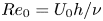 $Re_0 = U_0 h/\nu$, where
 $U_0$ is the laminar centreline velocity,
 $h = L_y/2$ half the domain height,
 $\nu$ the kinematic viscosity,
 $\mu$ the control strength as in (3.5) and
 $\delta \boldsymbol {u}$ the perturbation about the respective operating point
 $\boldsymbol {u}^*$. The adjustment rate in (3.5) is
 $\gamma = 1$ in all cases. The control type
 $\textrm {d}P/\textrm {d}x$ refers to the pressure-based control given in (3.3)–(3.6), while that labelled
 $v_e^*$ refers to the control along the dual vector of the unstable direction implemented according to (3.5), (3.6) and (3.14). The number of Fourier modes in the
 $x$ and
 $z$-directions,
 $N_x$ and
 $N_z$, contain the dealiased modes.

The construction of the adjoint feedback procedure requires access to the stable, neutral and unstable subspaces of the uncontrolled system. The corresponding eigenmodes of the Jacobian of the uncontrolled system were calculated by Arnoldi iteration and marginal and stable eigenmodes were subsequently used to construct the dual basis. Stability analyses of the pressure-controlled system were also carried out using the Arnoldi method.
4.1. Operating points: travelling waves in channel flow
The invariant solutions we wish to stabilise are travelling waves with one unstable direction, they are edge states in minimal flow units, which have been obtained by means of edge tracking in simulations with constant pressure gradient. In general, constant-flux simulations with variable pressure gradient are closer to experimental conditions, especially in small domains. For travelling-wave solutions this issue is mitigated as they are relative fixed points and thus have no dynamics. As such, travelling-wave solutions obtained with the constant-flux constraint result in a constant pressure gradient.
The structures differ in their spatial localisation and their degree of symmetry. The first one, TW1, has been calculated at  $Re_0 = 1394$ in a domain of size
 $L_x/h \times L_y/h \times L_z/h = 2 {\rm \pi}\times 2 \times 2{\rm \pi}$ (Zammert & Eckhardt Reference Zammert and Eckhardt2014) and is an edge state in the full space. It is localised in the spanwise direction, with two low-speed streaks accompanied by four vortices and is mirror symmetric about the midplane. The second one, TW-sym, has been obtained by a Newton–Krylov search at
 $Re_0 = 1010$ from an ECS in the domain
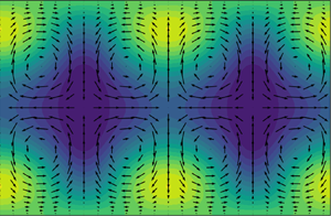
 $L_x/h \times L_y/h \times L_z/h = 2 {\rm \pi}\times 2 \times {\rm \pi}$ that had originally been calculated with constant flow rate (Zammert & Eckhardt Reference Zammert and Eckhardt2015). It consists of two high-speed streaks, four low-speed streaks and eight vortices and is not localised in the spanwise direction. Visualisations of the streamwise-averaged structures and their respective leading unstable eigenmode are presented in figures 4 and 5, respectively, where the colour coding represents the streamwise velocity component and the superimposed arrows the cross-flow.
Visualisation of the edge states showing the deviation of the streamwise average of the streamwise velocity component,  $\langle u \rangle _x$ from the laminar profile. The cross-flow
 $(v,w)$ is indicated by the superimposed arrows. (
 $a$) Edge state at
 $Re_0 = 1394$, (
 $b$) edge state at
 $Re_0 = 1010$ calculated in its symmetry-invariant subspace.

Visualisation of the unstable eigenmodes of TW1 ( $a$) and TW-sym (
 $b$) showing the deviation of the streamwise average of the streamwise velocity component,
 $\langle u \rangle _x$ from the laminar profile. The cross-flow
 $(v,w)$ is indicated by the arrows.

TW-sym is an edge state in a symmetry-invariant subspace, that is, a subspace invariant under the action of a symmetry group, only. Calculations of TW-sym are therefore carried out in a subspace that enforces mirror symmetry about the midplane ( $y=0$) and in the spanwise direction about the plane
 $z = {\rm \pi}/2$
 \begin{gather} s_y\left((u,v,w)^t(x,y,z)\right) = (u,-v,w)^t(x,-y,z), \end{gather}
 \begin{gather} s_z\left((u,v,w)^t(x,y,z)\right) = (u,v,-w)^t(x,y,-z), \end{gather}
where the superscript denotes the transpose. Invariant solutions obtained in symmetry-invariant subspaces are also solutions with respect to the unrestricted dynamics, where the number of unstable directions is usually higher (Duguet et al. Reference Duguet, Willis and Kerswell2008b; Kreilos & Eckhardt Reference Kreilos and Eckhardt2012; Avila et al. Reference Avila, Mellibovsky, Roland and Hof2013). In this context it is therefore of interest to assess the effect of symmetry-invariant calculations on feedback stabilisation. For this reason, we also carried out controlled simulations of TW1 within its symmetry-invariant subspace. More precisely, the symmetry-invariant subspaces here are subspaces of the full domain invariant under the transformations defined in (4.1) and (4.2) for TW-sym or, in case of TW1, in (4.1) only.
5. Stabilisation
5.1. Pressure-based control
Figure 6 presents phase-space trajectories of the controlled system for perturbations about TW1 and TW-sym with  $\|\boldsymbol {u}\|_2$, the friction factor
 $C_f = 2\tau _w/(\rho U_0^2)$, where
 $\tau _w$ is the shear stress at the bottom wall, and the cross-flow energy
 \begin{equation} Ecf(t) = \frac{1}{L_xL_yL_z}\int_0^{L_x} \int_{{-}L_y/2}^{L_y/2} \int_0^{L_z}\,\textrm{d}x\,\textrm{d}y\,\textrm{d}z \ \left(v^2(x,y,z,t) + w^2(x,y,z,t)\right), \end{equation}
as functions of the control parameter  $R$, i.e. series TW1-A, TW1-B, TW-sym-A and TW-sym-B in table 1. Figures 6(a) and 6(b) correspond to results for series TW1-A and TW1-B, respectively and figures 6(c) and 6(d) for TW-sym-A and TW-sym-B, respectively. Figures 6(a)–6(d) contain datasets from simulations carried out with different values of the control strength
 $\mu$ indicated by the colour gradient, where darker colours correspond to higher values of
 $\mu$ and hence stronger control. The corresponding control lines, which must intersect at the operating point, are shown in black. As can be seen from the data shown in the two panels, the feedback control results in phase-space trajectories where the perturbed edge state is driven towards the operating point for all observables. In the case of TW1-A, the trajectories resemble those from the model system discussed in § 3.1 and shown in figure 2. For the friction factor (TW1-B), the trajectories first approach intermediate states on the control line and subsequently follow the control line towards the operating point. For TW-sym-A the trajectories show large excursions and eventually return to the operating point, while for TW-sym-B the dynamics evolves along the control lines. We note that the trajectory passing through the point
 $R=0$ as in figure 6(
 $a$) does not necessarily result in laminar flow. At this point the control input cancels the reference pressure gradient, resulting in an instantaneously vanishing production term for the deviations of the laminar profile. However, deviations from the laminar profile can still be present in the flow. Relaminarisation may occur if the time scale at which the control acts is much larger than the time scale for the free decay of the cross-flow.
Phase-space trajectories for three different values of the control strength  $\mu$ according to table 1 and different observables obtained from controlled DNSs according to (3.3)–(3.6). (
 $a$) TW1,
 $L_2$-norm; (
 $b$) TW1, friction factor
 $C_f$; (
 $c$) TW-sym,
 $L_2$-norm; (
 $d$) TW-sym, cross-flow energy
 $Ecf$. All calculations targeting TW-sym have been carried out in the symmetry-invariant subspace introduced in § 4.

The simulations shown in figure 6 reached close vicinity of the operating point after very short simulation times (approximately  $20$ time units for norm-controlled simulations and approximately
 $50$ time units for friction-controlled simulations) of both TW1 and TW-sym. However, if the controlled system is evolved for very long times, the trajectories leave the operating point again. This is demonstrated by the time evolution of
 $\|\boldsymbol {u}\|_2$ shown in red (light grey) and
 $C_f$ shown in blue (dark grey) in figure 7(
 $a$) for the operating point TW1. A deviation of
 $\|\boldsymbol {u}\|_2$ from the reference value is visible after approximately 1000 time units, while
 $C_f$ appears to remain constant. Figure 7(
 $b$) presents the time evolution of the cross-flow energy with
 $v$ and
 $w$ being the wall-normal and spanwise components of
 $\boldsymbol {u} = (u,v,w)$. The control is unable to prevent the dynamics from escaping from the operating point towards the laminar fixed point. Interestingly, this happens on a much shorter time scale compared to the departure of the control observables from their target values. Similar observations can be made for the dynamics of TW1 controlled with respect to
 $C_f$, for TW-sym and for controlled simulations of TW1 carried out in its symmetry-invariant subspace (not shown).
Time evolution of the control observables ( $a$) and the cross-flow energy (
 $b$) for the pressure-controlled simulations with target state TW1. Dynamics controlled with respect to the
 $L_2$-norm with
 $\mu = 10^6$ and with respect to
 $C_f$ with
 $\mu = 3 \times 10^6$ shown in red (grey) and blue (dark grey), respectively.

The results shown in figure 7 suggest the presence of a residual instability in the controlled simulations. According to the discussion in § 2.2, an instability in the controlled system could result from the control being too weak to completely remove the original instability, from the control being orthogonal to the unstable direction as would be the case for strictly periodic instabilities or from an undesired destabilising effect of the control on the stable directions. The first possibility can be ruled out by an exhaustive parameter scan. The second possibility does not apply either, as the unstable directions have non-zero streamwise mean as discussed in § 4.1 and thus overlap with the control. In what follows we therefore investigate in detail how the control alters the tangent space structure of the chosen invariant solutions.
5.1.1. Effect of the control on stable and unstable directions
In order to quantify the effect of the control on the tangent space of the invariant solutions investigated here, stability analyses of TW1 with respect to the coupled system consisting of DNS and feedback control as in (3.3)–(3.6) have been carried out, see series TW1-A-stab listed in table 1. Figure 8 shows the eigenvalues of the Jacobian at TW1 for the free dynamics and for the  $L_2$-norm controlled system for different values of the control strength
 $\mu$. As can be seen, the free dynamics is such that TW1 has one unstable direction as expected for an edge state. For low values of
 $\mu$ the corresponding single positive real eigenvalue decreases with increasing
 $\mu$. At the same time, a pair of complex conjugate eigenvalues with negative real part move closer to the line where the latter vanishes. Eventually, their real part becomes positive, indicating the presence of a new unstable direction. For a small set of parameters, both old and new unstable directions are present. That is, even though the original unstable direction is removed for large enough
 $\mu$, the control indeed destabilises stable directions of the uncontrolled system. The neutral directions associated with continuous shift symmetries remain unaffected, as can be seen by considering the eigenvalues with zero real parts in figure 8.
Spectrum of the Jacobian at TW1 for the combined system DNS with feedback control according to (3.3)–(3.6) as a function of the control strength  $\mu$. The thick black dots correspond to the uncontrolled system and the decreasing colour gradient indicates increasing values of
 $\mu$. The positive real eigenvalue corresponding to the original instability decreases with increasing
 $\mu$ and eventually changes sign by jumping from 0.005 to
 $-$0.0025 on the real axis. With increasing
 $\mu$ a new feedback-induced instability occurs, represented by the complex eigenvalues with positive real parts.

Willis et al. (Reference Willis, Duguet, Omel'chenko and Wolfrum2017) also calculated eigenvalues and Floquet exponents for their successfully stabilised invariant solutions. In both cases there are stable eigenvalues whose real parts move closer to zero in the controlled system, see figure 3( $a$) of Willis et al. (Reference Willis, Duguet, Omel'chenko and Wolfrum2017) for the spectrum of a travelling wave, and figure 4(
 $c$) for the Floquet exponents of a stabilised periodic orbit. In summary, a simple 1-D feedback control can have adverse effects on the stable directions, whereby the real parts of the stable eigenvalues tend to zero and may even become positive, as shown here. This precludes the application of the pressure-based feedback control to the search for new invariant solutions in channel flow following the procedure proposed by Willis et al. (Reference Willis, Duguet, Omel'chenko and Wolfrum2017) for pipe flow, as without any information about eventual overlaps between the control and the stable directions it is difficult to know a priori if such a feedback-induced instability indeed occurs. Hence a black-box application of such feedback strategies without good knowledge of the coefficients is not guaranteed to work. Before returning to this point in more detail in the following section, we briefly discuss the experimental applicability of this method in terms of turbulence control.
5.1.2. Potential experimental applicability
Although the feedback control does not stabilise the operating point, it is able to find global target observables connected with the streamwise component of the flow, which do not require knowledge of all velocity components and are thus easier accessible experimentally. This suggests that the proposed pressure-based feedback control can be used to confine turbulent dynamics to a region of phase space selected by a given value of e.g. the friction factor and to prevent large fluctuations in kinetic energy or drag. Preliminary results for a wall-suction-based feedback control for plane Couette flow (Linkmann & Eckhardt Reference Linkmann and Eckhardt2019) show that this is indeed the case, at least in small domains. This suggests that further research into the effect of pressure-based linear feedback on the global properties of a flow may be worthwhile pursuing. In order to fully assess the potential experimental viability of such an approach, it is of paramount importance to carry out numerical simulations in domains with large streamwise extent, far beyond the minimal flow units used in the present study.
5.2. Adjoint control
Figure 9 shows phase-space trajectories with respect to the  $L_2$-norm and the cross-flow energy and time series of the latter obtained with the control implemented according to (3.14) and (3.4)–(3.6) for TW1, i.e. series TW1-C and TW1-D summarised in table1. Figures 9(a) and 9(c) correspond to DNS controlled with respect to
 $L_2$-norm and figures9(b) and 9(d) to controlled runs with respect to the cross-flow energy. As can be seen from the phase-space trajectories in figures 9(a) and 9(b), all controlled simulations approach the targeted values of the chosen observables, as has been the case for the streamwise-invariant control discussed in the beginning of § 5. The timeevolution of the cross-flow energy (figures 9c and 9d) indicates that the controlled system now also approaches the actual operating point and stays in its vicinity for approximately 200 time units for the
 $L_2$-norm control and for over 300 time units for cross-flow control. However, eventually the state-space trajectory leaves the operating point again, as can be seen in the time evolution shown in figure 9(c), for instance. The reason for this is most likely due to the choice of observable and thus with the control input. According to § 3.2, the gradient of the input function
 $\kappa$ at the operating point must be colinear with the unstable direction to achieve stabilisation. The results here suggest the presence of small overlaps. We will come back to this point later.
TW1: phase-space trajectories ( $a{,}b$) and corresponding evolution of the cross-flow energy (
 $c{,}d$) for two different values of the control strength
 $\mu$ for the adjoint-based control procedure given by (3.14) and (3.4)–(3.6) with respect to the
 $L_2$-norm (
 $a{,}c$, series TW1-C) and the cross-flow energy (
 $b{,}d$, series TW1-D). The control lines are indicated in black.

Results from controlled simulations targeting TW-sym, all of which have been carried out in the symmetry-invariant subspace introduced in § 4, that is, series TW-sym-C in table 1, are presented in figure 10. Here, stabilisation has been achieved using the  $L_2$-norm as an observable, as can be seen from the phase-space trajectories of runs TW-sym-C3, TW-sym-C4 and TW-sym-C5 in figure 10(
 $a$) and the corresponding evolution of the cross-flow energy in figure 10(
 $c$). Compared with the controlled dynamics targeting TW1 carried out in the full space and shown in figure 9, the approach to the operating point is much slower, but the stabilisation is complete. For low values of the control strength
 $\mu$, i.e. for runs TW-sym-C1 and TW-sym-C2, the controlled dynamics gets trapped into new invariant tori, where the mean values of the
 $L_2$-norm and the cross-flow energy depend on
 $\mu$ as shown by the phase-space plots and the time evolution of the cross-flow energy in figures 10(c) and 10(d). In all cases the phase-space trajectories shown in figure 10 remain in the vicinity of the control lines, that is, the control procedure confines the dynamics to regions phase space close to the chosen control lines.
TW-sym: phase-space trajectories ( $a{,}b$) and corresponding evolution of the cross-flow energy (
 $c{,}d$) for different values of the control strength
 $\mu$ for the adjoint-based control procedure given by (3.14) and (3.4)–(3.6) with respect to the
 $L_2$-norm ((
 $a{,}c$) TW-sym-C3-C5, (
 $b{,}d$) TW-sym-C1-C2 of table 1). The green ellipsoids in (
 $b$) shows new limit cycles/invariant tori in the controlled dynamics of TW-sym-C1 and TW-sym-C2. These are also shown in the insets in energy input (
 $I$) – dissipation (
 $D$) coordinates. The control lines are indicated in black. All calculations have been carried out in the symmetry-invariant subspace introduced in § 4.

According to the discussion in § 3.2, the success of the adjoint method depends on the choice of feedback function  $\kappa$, which in turn depends on the choice of observable. Concerning the choice of observable, several observations can be made from a comparison of the visualisations of the ECS in figure 4 and those of their respective unstable directions shown in figure 5. For both structures we note that the cross-flow varies very little between the ECS and its unstable direction, while clear differences are visible in the streamwise velocity component at least for TW1. This suggests that the cross-flow energy should work better than the
 $L_2$-norm as a control observable for TW1, which is indeed the case, as can be seen by comparison between figures 9(
 $c$) and 9(
 $d$). For TW-sym the
 $L_2$-norm worked well. Finally, we note that stabilisation through the adjoint-based feedback strategy could not be achieved using the friction factor
 $C_f$ as an observable. Since
 $C_f$ is linear in the velocity field, its gradient at the operating point is a constant vector and its dual hence not orthogonal to all stable directions. The high degree of symmetry enforced by the calculations in the symmetry-invariant subspace facilitates stabilisation, as it only allows instabilities that are shift-and-reflect symmetric, as is the target state itself. As such, an overlap between the gradient of
 $\kappa$ at the operating point and the unstable direction is much easier to achieve, as they share the same symmetries. This sensitivity highlights some of the limitations of global 1-D feedback control to stabilise exact coherent structures.
A few words on the performance limits, convergence and robustness of the control protocol are in order. Firstly, as the control procedure is based upon the linearised Navier–Stokes equations, it is designed to work in a neighbourhood of the operating point. In order to assess the performance limit of the proposed controller, we carried out a parameter scan varying the magnitude of the random perturbation  $\delta \boldsymbol {u}$ at a fixed value of
 $\mu$. We found that the control protocol was successful for
 $\| \delta \boldsymbol {u}\|_2 / \| \boldsymbol {u}^*\|_2 < 0.25$, where
 $\boldsymbol {u}^*$ denotes the operating point (not shown). Second, the dual unit vectors
 $v_e^*$ used in the calculations have been obtained approximatively by calculating the dual basis of a subspace spanned by the unstable eigenmode, the neutral eigenmodes and the first 40 stable eigenmodes, ordered by decreasing Lyapunov exponent. For a smaller number of unstable eigenmodes, the controlled dynamics did not recover edge state. Instead, it resembles that obtained for weak values of the control strength shown in figures10(b) and 10(d), i.e. stable oscillatory solutions of the dynamical system given by (3.14) and (3.4)–(3.6) were obtained. Using a larger number of stable modes results in faster stabilisation as shown in figure 11 for example calculations of TW-sym-C3 using dual bases calculated with respect to 40, 50 and 60 stable eigenmodes. Third, calculations on finer grids require a more accurate calculation of the dual basis, i.e. with respect to a higher-dimensional approximation of the solution's stable subspace. For instance, increasing the resolution from 48 to 64 Fourier modes in the homogeneous directions required the dual basis to be calculated with respect to at least 80 stable directions to stabilise TW-sym (not shown).
Phase-space trajectories ( $a$) and corresponding evolution of the cross-flow energy(
 $b$) for TW-sym-C3 using the control procedure given by (3.14) and (3.4)–(3.6) with respect to the
 $L_2$-norm. The dual basis used in the control law has been calculated with respect to 40 (black), 50 (blue/dark grey) or 60 (red/light grey) stable eigenmodes.

6. Discussion and conclusions
In this paper we considered the application of linear feedback control as a strategy to stabilise invariant solutions of the Navier–Stokes equations. As an example of a canonical shear flow with a subcritical transition to turbulence, we considered channel flow at Reynolds numbers below the onset of linear instability at  $Re = 5772.22$. We focussed on the simplest possible problem, the stabilisation of edge states in minimal flow units, here, travelling waves with one unstable direction. Using explicitly constructed feedback strategies, the aim of the study was to point out and discuss the issues that arise when applying linear feedback control in attempts to stabilise exact coherent structures. We devised two feedback control procedures. The first one is pressure based, and thus in principle experimentally viable. The second one is constructed to remain orthogonal to the contracting and neutral subspaces of the target state's tangent space. As it cannot be implemented in the laboratory, it mainly serves to highlight the complications that arise, in particular in comparison with the pressure-based method. Simulations of the controlled systems were carried out for two target states that differ in their respective degrees of spanwise localisation. In case of the de-localised state, all calculations were carried out in its symmetry-invariant subspace.
The pressure-based control strategy was inspired by the work of Willis et al. (Reference Willis, Duguet, Omel'chenko and Wolfrum2017) on feedback stabilisation of edge states in pipe flow, where the viscosity was adjusted as a function of energy-type observables. In order to obtain a control procedure that, in principle, can be carried out experimentally, we proposed to adjust the pressure gradient instead of the viscosity as a function of either energy-type observables or the friction factor. Even though the control resulted in the dynamics approaching the respective target values of the observables used in the control strategy, the actual edge states were not stabilised as the control procedure has a destabilising effect on some of the structures’ contracting directions. This highlights that the success of similar methods such as that proposed by Willis et al. (Reference Willis, Duguet, Omel'chenko and Wolfrum2017) strongly depends on the system parameters and cannot be guaranteed to work in general. Stabilisation can be achieved if the control acts along the dual vector of the original unstable direction, that is, on a hyperplane orthogonal to all stable and neutral directions. Here, it was found that care must be taken in the choice of observable, because the latter results in different control input terms whose gradients may or may not overlap with the stable directions. However, we found that for standard energy-type observables such as the  $L_2$-norm or the energy of the transverse fluctuations, only the de-localised and highly symmetric target state was stabilised, while for the spanwise localised target states the state-space trajectory of the controlled system remained very close to the target state for an extended time interval. This emphasises the limitations of global 1-D feedback in the present context.
Apart from the observations summarised above, a few further issues deserve further attention in this context as they present obstacles that need to be addressed when designing linear closed-loop control strategies for the stabilisation of exact coherent structures.
First, domains with periodic directions allow continuous symmetries in form of shifts along these directions, resulting in neutral modes with zero mean given by the derivatives of the target state in these directions, see e.g. Wolfe & Samelson (Reference Wolfe and Samelson2006). For the specific pressure-driven feedback this complication does not occur as the pressure gradient is constant in both streamwise and spanwise directions and therefore orthogonal to all modes with zero mean. However, generally speaking, this issue needs to be taken into account in the design of linear control strategies applied to systems with continuous symmetries, in particular as neutral modes can be quickly destabilised by the control. It may arise, for instance, in control strategies that directly modulate the flow. The adjoint-based method takes care of this problem by construction, with the important drawback that they can only be used in numerical simulations. This raises the general question as to how to design a practically relevant control strategy in systems with continuous symmetries that either leaves the neutral subspace unaffected or stabilises also the neutral modes of the uncontrolled system.
Second, a successful control strategy should in principle be applicable for a range of Reynolds numbers. Considering specifically the stabilisation of edge states in the wider context of turbulence control, the fact that edge states in plane Poiseuille flow disappear at Reynolds numbers above the laminar stability threshold limits the applicability of the methods proposed here to unsteady, but not turbulent, channel flow at subcritical Reynolds numbers. However, similar complications arise also for shear flows like pipe or plane Couette flow where the laminar profile is linearly stable at all  $Re$. An important challenge for the application of linear closed-loop control to stabilise invariant solutions is connected with the contraction of the basins of attraction. In pipe or plane Couette flow, the basin of attraction of the laminar profile contracts with increasing
 $Re$. A similar effect occurs for a stabilised exact coherent structure, its basin of attraction will contract with increasing
 $Re$ and domain size. For the controlled system, the situation is even more challenging as the increasing degree of instability requires higher feedback gain, resulting potentially in a further contraction of the basin of attraction of the invariant solution.
Third, flow control is ultimately focussed on questions of practical relevance. In the present context, this includes the combination of feedback control with classical methods for finding and continuing invariant solutions. For linear control to be practically relevant, two conditions have to be satisfied: (i) the target state has to lie in the ergodic region of state space, i.e. it should be approached closely by turbulent trajectories of the open-loop flow and (ii) turbulent trajectories of open-loop flow should approach the target state to within a distance smaller than the size of its region of attraction for closed-loop flow on practically accessible time scales.
Having discussed the challenges and limitations of global 1-D feedback in the context of invariant solutions, we now briefly mention applications where such strategies would (i) either be applicable as they are or with minor modifications, or (ii) where stabilisation of specific invariant solutions would be very useful.
Even though the pressure-based method fails as a means to stabilise invariant solutions, it is shown to target set values of the  $L_2$-norm, the cross-flow energy or the friction factor. As such, pressure-based dynamic feedback may be a useful tool to accelerate or prevent relaminarisation events. Since feedback strategies alter the stability of an exact solution to the Navier–Stokes equations, they cannot only be used to stabilise an operating point, but also to further destabilise it, if so desired, or to confine the dynamics to a certain region in phase space. This may be useful in systems where there is an interest in avoiding certain flow states, e.g. those with enhanced drag. Here, the issues discussed earlier are mitigated by the fact that the controller only needs to be efficient when the state-space trajectory approaches a small neighbourhood of the undesired state.
Recent results from numerical simulations of channel flow suggest that extreme fluctuations in the streamwise component of the wall shear stress are less likely if the flow is maintained by prescription of a constant flow rate compared with forcing through a constant pressure drop or a fixed energy input (Quadrio, Frohnapfel & Hasegawa Reference Quadrio, Frohnapfel and Hasegawa2016); however, the differences concerned rare events. Dynamic feedback could be a possibility to avoid extreme fluctuations more effectively. In particular for shear flows with a pair of exact coherent structures born in a saddle-node bifurcation, typical extreme events should correspond to the state-space trajectory following the heteroclinic connection from the lower to the upper branch. Stabilising states on the lower branch is an efficient way to suppress such extreme events. Farazmand & Sapsis (Reference Farazmand and Sapsis2019) showed that extreme events in 2-D Kolmogorov flow can be avoided by dynamically regulating the dynamics of certain Fourier modes at the driving scale. Preliminary results show that a variant of the pressure-based feedback strategy proposed here can be applied to damp transverse fluctuations in plane Couette flow through adjustable wall suction (Linkmann & Eckhardt Reference Linkmann and Eckhardt2019). This calls for further investigations using in particular the pressure-based control strategy.
Acknowledgements
With great sadness we report that B. Eckhardt passed away shortly before finalisation of this manuscript. We thank him for his astute scientific insight and thoughtful guidance. M.L. thanks Y. Duguet for very helpful discussions and the anonymous referees for their constructive feedback that has significantly improved the quality of the manuscript.
Declaration of interests
The authors report no conflict of interest.



