1 Introduction
Perhaps the simplest way to produce a thin liquid film is to deposit a layer of liquid onto a substrate via withdrawal from a liquid pool. The physics of the process is known as the drag-out problem or the Landau–Levich problem, after pioneering studies by Landau & Levich (Reference Landau and Levich1942). The corresponding prototypical dip coating flow is popular not only in laboratory experiments (Scriven Reference Scriven1988) but also in industry (Schunk, Hurd & Brinker Reference Schunk, Hurd and Brinker1997) because of its simplicity. Dip coating and related methods are sufficiently flexible to produce films on different geometries (Bretherton Reference Bretherton1961; Wilson Reference Wilson1982; Park & Homsy Reference Park and Homsy1984; de Ryck & Quéré Reference de Ryck and Quéré1996) and can be applied to fluids with various properties (Krechetnikov & Homsy Reference Krechetnikov and Homsy2005, Reference Krechetnikov and Homsy2006; Afanasiev, Münch & Wagner Reference Afanasiev, Münch and Wagner2007; Dixit & Homsy Reference Dixit and Homsy2013a ,Reference Dixit and Homsy b ; Javidi, Pope & Hrymak Reference Javidi, Pope and Hrymak2016; Maillard et al. Reference Maillard, Bleyer, Andrieux, Boujlel and Coussot2016). The study of Landau & Levich (Reference Landau and Levich1942) can be also extended to related systems such as the formation of Marangoni-driven films on a heated substrate partially immersed in a liquid pool (Münch Reference Münch2002; Münch & Evans Reference Münch and Evans2005, Reference Münch and Evans2006).
In dip coating, the constant film thickness
 $h_{\infty }^{\ast }$
is determined by the balance between the viscous drag, surface tension, gravity and inertia; and characterised as a function of the capillary number
 $Ca$
defined as
 $\unicode[STIX]{x1D707}u_{s}/\unicode[STIX]{x1D70E}$
, where
 $\unicode[STIX]{x1D707}$
is the fluid viscosity,
 $u_{s}$
is the substrate speed and
 $\unicode[STIX]{x1D70E}$
is the surface tension. For Newtonian fluids, Landau & Levich (Reference Landau and Levich1942) determined
 $h_{\infty }^{\ast }$
for low
 $Ca$
at which gravitational drainage can be negligible. A number of authors extended the study of Landau & Levich (Reference Landau and Levich1942) by including gravitational drainage (White & Tallmadge Reference White and Tallmadge1965; Spiers, Subbaraman & Wilkinson Reference Spiers, Subbaraman and Wilkinson1974; Wilson Reference Wilson1982), inertia (Kheshgi, Kistler & Scriven Reference Kheshgi, Kistler and Scriven1992; de Ryck & Quéré Reference de Ryck and Quéré1998) or the normal viscous stress at the meniscus (Spiers et al.
Reference Spiers, Subbaraman and Wilkinson1974; Esmail & Hummel Reference Esmail and Hummel1975b
) in their studies.
Numerical analyses (e.g. finite element (FE) or finite volume computations) have also been commonly used to determine
 $h_{\infty }^{\ast }$
because no simple film-thickness-predicting equation covers low to high
 $Ca$
and to extend the study to complex fluids (Réglat, Labrie & Tanguy Reference Réglat, Labrie and Tanguy1993; Jin, Acrivos & Münch Reference Jin, Acrivos and Münch2005; Jenny & Souhar Reference Jenny and Souhar2009; Campana et al.
Reference Campana, Ubal, Giavedoni and Saita2010; Abedijaberi et al.
Reference Abedijaberi, Bhatara, Shaqfeh and Khomami2011; Filali, Khezzar & Mitsoulis Reference Filali, Khezzar and Mitsoulis2013).
Most of the previous studies on dip coating, including those referred to earlier, have considered withdrawal of a substrate in the direction opposite to gravity from an sufficiently large pool. In this unconfined dip coating system, most of the pool remains virtually static, except in the small region near the moving substrate, where the flow can be recognised inside the extremely curved meniscus viewed in the far field (Krechetnikov & Homsy Reference Krechetnikov and Homsy2006). However, the results of those studies cannot be directly applied to many practical situations in which the pool is confined, such as a coating on fibre (Quéré Reference Quéré1999) or laboratory experiments (Ahn et al. Reference Ahn, Kim, Kim and Nam2015). Although Kheshgi et al. (Reference Kheshgi, Kistler and Scriven1992) considered a confined pool in the dip coating problem, his study considered a meniscus distortion due to an obstacle near the static meniscus.
In the present study, we define the confined pool as a pool where the stationary container wall parallel to the substrate has an effect on the film thickness and forms a channel with the substrate. There are, however, no limitations along the withdrawal direction, as in the usual unconfined dip coating. In a confined dip coating system, two clearly distinct flow regimes appear depending on the capillary number
 $Ca$
: the meniscus-controlled regime for low
 $Ca$
and the channel-controlled regime for high
 $Ca$
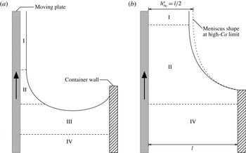
. Typical dip coating flows under these regimes are shown schematically in figure 1. The film thickness is dominantly controlled by the meniscus shape in the meniscus-controlled regime and by the channel width, which is defined as the distance between the substrate and the stationary wall, in the channel-controlled regime. Both regimes exhibit distinct scaling behaviours. We analysed these behaviours theoretically and numerically. The results of the present study can be used to predict the film thickness entrained from a confined pool that can be encountered in thin-film productions in industry or laboratory experiments.
Schematic of confined dip coating system for (a) meniscus-controlled regime and (b) channel-controlled regime. (a) For the flow in the meniscus-controlled regime, i.e. the region excluding the regions close to the moving plate (I and II), the liquid is virtually stationary (III and IV). (b) For the channel-controlled regime, the static pool disappears, and the dynamic meniscus region (II) fills the channel. The dotted line represents the meniscus shape at the high-
 $Ca$
limit. See appendix A for a discussion of region IV.

2 Formulation of problem
In dip coating problems, the flow can be divided into three regions: the film entrainment region (region I), the dynamic meniscus region (region II) and the static meniscus region (region III), as shown in figure 1. In the film entrainment region, the deposited liquid film translates along the moving plate. The characteristic length
 $l_{f}$
for this region can be easily determined by considering the balance between the viscous and gravitational forces. In the static meniscus region, the meniscus shape in that region is determined by the balance between the capillary and gravitational forces. A simple force balance analysis also yields the characteristic length
 $l_{c}$
, known as the capillary length. The aforementioned two regions are connected by the dynamic meniscus region where the dynamic effects due to liquid in motion should be considered. In this region, the meniscus shape is set by the balance between the viscous drag, surface tension and gravity, provided inertia is absent. The meniscus profile along the moving plate determines the constant film thickness
 $h_{\infty }^{\ast }$
. In addition to the aforementioned three regions, when a pool is confined, the channel region (region IV) appears far below the meniscus, and the characteristic length of this region is the channel width
 $l$
. The flow in this region is fully developed as described in appendix A.
For unconfined dip coating, Landau & Levich (Reference Landau and Levich1942) determined
 $h_{\infty }^{\ast }$
at a low capillary number
 $Ca$
, under which gravitational drainage is negligible, as
 $$\begin{eqnarray}h_{\infty }^{\ast }=0.9458l_{c}Ca^{2/3}=0.9458l_{f}Ca^{1/6}.\end{eqnarray}$$
 $l_{c}\equiv \sqrt{\unicode[STIX]{x1D70E}/\unicode[STIX]{x1D70C}g}$
or
 $l_{f}\equiv \sqrt{\unicode[STIX]{x1D707}u_{s}/\unicode[STIX]{x1D70C}g}$
has been employed as the characteristic length of the flow, where
 $\unicode[STIX]{x1D70C}$
is the liquid density and
 $g$
is the gravitational acceleration. These characteristic lengths imply that gravity has a significant influence on unconfined dip coating flows. The power-law dependence on
 $Ca$
varies depending on the choice of characteristic length. Several authors have chosen
 $l_{c}$
as the characteristic length (Campana et al.
Reference Campana, Ubal, Giavedoni and Saita2010; Dixit & Homsy Reference Dixit and Homsy2013a
), whereas others have employed
 $l_{f}$
(White & Tallmadge Reference White and Tallmadge1965; Esmail & Hummel Reference Esmail and Hummel1975b
; Weinstein & Ruschak Reference Weinstein and Ruschak2001; Jin et al.
Reference Jin, Acrivos and Münch2005; Benilov & Zubkov Reference Benilov and Zubkov2008), depending on convenience for relevant analyses. However, we show that the channel width
 $l$
is the appropriate characteristic length for confined dip coating flows.
2.1 Dimensionless numbers
The fundamental problem of a confined dip coating system is determining the dependence of the film thickness
 $h_{\infty }^{\ast }$
on the system parameters (
 $l$
,
 $u_{s}$
and
 $g$
), and the physical properties of the fluid (
 $\unicode[STIX]{x1D70C}$
,
 $\unicode[STIX]{x1D707}$
and
 $\unicode[STIX]{x1D70E}$
). In the present study, it is assumed that a substrate is a flat plate and the coating liquid is a pure Newtonian fluid (i.e. there are no surfactants or particles) that wets the plate completely. For the flow where the foregoing assumptions are valid, the Buckingham
 $\unicode[STIX]{x03C0}$
theorem yields four dimensionless numbers describing the flow system uniquely. The numbers are the dimensionless thickness
 $T$
, the dimensionless channel width
 $L$
, the capillary number
 $Ca$
and the material number
 $m$
:
 $$\begin{eqnarray}T\equiv \frac{h_{\infty }^{\ast }}{l},\quad L\equiv \frac{l}{\sqrt{\unicode[STIX]{x1D70E}/\unicode[STIX]{x1D70C}g}},\quad Ca\equiv \frac{\unicode[STIX]{x1D707}u_{s}}{\unicode[STIX]{x1D70E}},\quad m\equiv \sqrt{\frac{\unicode[STIX]{x1D70C}\unicode[STIX]{x1D70E}^{3}}{g\unicode[STIX]{x1D707}^{4}}}.\end{eqnarray}$$
Note that three dimensionless numbers are required to define an unconfined dip coating flow uniquely (Tallmadge & Soroka Reference Tallmadge and Soroka1969); however, the newly introduced parameter, the channel width
 $l$
, generates the additional dimensionless number
 $L$
. Another important number, the Reynolds number
 $Re$
, can be obtained by the combination of the other numbers (2.2):
 $$\begin{eqnarray}Re\equiv \unicode[STIX]{x1D70C}u_{s}h_{\infty }^{\ast }/\unicode[STIX]{x1D707}=mTLCa.\end{eqnarray}$$
Here, we limit our study to a Stokes flow (
 $Re\ll 1$
);
 $T$
is solely determined by
 $Ca$
and
 $L$
. Accordingly, we set the value of
 $m$
to
 $10^{-5}$
in FE computations. Under this condition, we can assume a confined dip coating flow to be a Stokes flow because we explore the range in
 $Ca$
up to
 $10^{2}$
such that
 $Re\simeq mCa$
.
2.2 Governing equations and boundary conditions
We consider a steady flow in a confined dip coating system where the flat plate moves vertically with a constant velocity
 $\boldsymbol{v}_{s}^{\ast }$
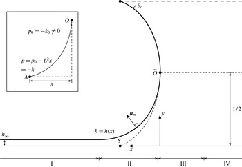
(the asterisk denotes the corresponding dimensional variables throughout the present paper), as shown in figure 2, and only the part of the meniscus closer to the moving plate is examined in the present study. When the inertia is negligible, the flow is governed by the Stokes equations:
 $$\begin{eqnarray}\displaystyle & \unicode[STIX]{x1D735}^{\ast }\boldsymbol{\cdot }\boldsymbol{v}^{\ast }=0, & \displaystyle\end{eqnarray}$$
 $$\begin{eqnarray}\displaystyle & \unicode[STIX]{x1D735}^{\ast }\boldsymbol{\cdot }\unicode[STIX]{x1D64F}^{\ast }+\unicode[STIX]{x1D70C}\,\boldsymbol{g}=\mathbf{0}, & \displaystyle\end{eqnarray}$$
where
 $\boldsymbol{v}^{\ast }$
is the velocity,
 $\unicode[STIX]{x1D64F}^{\ast }$
is the total stress tensor and
 $\boldsymbol{g}$
is the gravitational field. The no-slip conditions at the moving plate and stationary wall are
 $$\begin{eqnarray}\displaystyle & \boldsymbol{v}^{\ast }=\boldsymbol{v}_{s}^{\ast }\quad \text{at}\;y^{\ast }=0, & \displaystyle\end{eqnarray}$$
 $$\begin{eqnarray}\displaystyle & \boldsymbol{v}^{\ast }=\mathbf{0}\quad \text{at}\;y^{\ast }=l. & \displaystyle\end{eqnarray}$$
The stress balance and the kinematic condition at the meniscus are
 $$\begin{eqnarray}\displaystyle & \boldsymbol{n}_{m}\boldsymbol{\cdot }\unicode[STIX]{x1D64F}^{\ast }=\unicode[STIX]{x1D70E}\unicode[STIX]{x1D705}_{}^{\ast }\boldsymbol{n}_{m}\quad \text{at}\;y^{\ast }=h^{\ast }(x^{\ast }), & \displaystyle\end{eqnarray}$$
 $$\begin{eqnarray}\displaystyle & \boldsymbol{n}_{m}\boldsymbol{\cdot }\boldsymbol{v}^{\ast }=0\quad \text{at}\;y^{\ast }=h^{\ast }(x^{\ast }), & \displaystyle\end{eqnarray}$$
where
 $\boldsymbol{n}_{m}$
is the outward unit normal vector and is given by
 $$\begin{eqnarray}\boldsymbol{n}_{m}=\left.\left(-\frac{\text{d}^{}h^{\ast }}{\text{d}^{}x^{\ast }}\boldsymbol{i}+\boldsymbol{j}\right)\right/\left[1+\left(\frac{\text{d}^{}h^{\ast }}{\text{d}^{}x^{\ast }}\right)^{2}\right]^{1/2},\end{eqnarray}$$
where
 $\boldsymbol{i}$
,
 $\boldsymbol{j}$
are the unit vectors in the positive directions of the axes; and
 $\unicode[STIX]{x1D705}_{}^{\ast }$
is the curvature of meniscus:
 $$\begin{eqnarray}\unicode[STIX]{x1D705}_{}^{\ast }=-\unicode[STIX]{x1D735}^{\ast }\boldsymbol{\cdot }\boldsymbol{n}_{m}.\end{eqnarray}$$
Here, we set the pressure on the gas side to zero. Finally, the stress tensor
 $\unicode[STIX]{x1D64F}^{\ast }$
of a pure Newtonian fluid is given by
 $$\begin{eqnarray}\unicode[STIX]{x1D64F}^{\ast }=-p^{\ast }\unicode[STIX]{x1D644}+\unicode[STIX]{x1D707}[\unicode[STIX]{x1D735}^{\ast }\boldsymbol{v}^{\ast }+(\unicode[STIX]{x1D735}^{\ast }\boldsymbol{v}^{\ast })^{\text{T}}],\end{eqnarray}$$
where
 $p^{\ast }$
is the pressure and
 $\unicode[STIX]{x1D644}$
is the identity tensor.
Formulation of the problem. All variables are scaled for the static meniscus region. A meniscus profile
 $h$
is represented as a function of the
 $x$
coordinate. The dotted curve represents an imaginary static meniscus with a contact angle
 $\unicode[STIX]{x1D703}_{c}$
in the absence of flow. The solid line represents the meniscus shape due to the flow. The meniscus shape deviates from the shape of the static meniscus in the dynamic meniscus region (region II). In the inset,
 $\unicode[STIX]{x1D705}_{0}$
is the curvature at the centre of the imaginary static meniscus and is discussed in § 3.

2.3 Dynamic meniscus region
In this region, the balance among the viscous drag, surface tension and gravity is important, and the scaling for variables need to be chosen appropriately to examine the balance. Following Park & Homsy (Reference Park and Homsy1984), we non-dimensionalise the Stokes equations and boundary conditions by the following scales:
 $$\begin{eqnarray}(x^{\ast },y^{\ast })\sim (lCa^{1/3},lCa^{2/3}),\quad (u^{\ast },v^{\ast })\sim (u_{s},u_{s}Ca^{1/3}),\quad p^{\ast }\sim \frac{\unicode[STIX]{x1D70E}}{l},\quad h^{\ast }\sim lCa^{2/3}.\end{eqnarray}$$
The variables in these scales are denoted by overbars, and the equations and conditions in the component form become
 $$\begin{eqnarray}\displaystyle & \displaystyle \frac{\unicode[STIX]{x2202}\overline{u}}{\unicode[STIX]{x2202}\overline{x}}+\frac{\unicode[STIX]{x2202}\overline{v}}{\unicode[STIX]{x2202}\overline{y}}=0, & \displaystyle\end{eqnarray}$$
 $$\begin{eqnarray}\displaystyle & \left.\begin{array}{@{}c@{}}\displaystyle Ca^{2/3}\frac{\unicode[STIX]{x2202}^{2}\overline{u}}{\unicode[STIX]{x2202}\overline{x}^{2}}+\frac{\unicode[STIX]{x2202}^{2}\overline{u}}{\unicode[STIX]{x2202}\overline{y}^{2}}-\frac{\unicode[STIX]{x2202}\overline{p}}{\unicode[STIX]{x2202}\overline{x}}-Ca^{1/3}L^{2}=0,\\ \displaystyle Ca^{4/3}\frac{\unicode[STIX]{x2202}^{2}\overline{v}}{\unicode[STIX]{x2202}\overline{x}^{2}}+Ca^{2/3}\frac{\unicode[STIX]{x2202}^{2}\overline{v}}{\unicode[STIX]{x2202}\overline{y}^{2}}-\frac{\unicode[STIX]{x2202}\overline{p}}{\unicode[STIX]{x2202}\overline{y}}=0,\end{array}\right\} & \displaystyle\end{eqnarray}$$
 $$\begin{eqnarray}\overline{u}=1,\quad \overline{v}=0\quad \text{at}\;\overline{y}=0,\end{eqnarray}$$
 $$\begin{eqnarray}\displaystyle & & \displaystyle \left.\begin{array}{@{}c@{}}\displaystyle 2Ca^{2/3}\frac{\text{d}^{}\overline{h}}{\text{d}^{}\overline{x}}\left(\frac{\unicode[STIX]{x2202}\overline{u}}{\unicode[STIX]{x2202}\overline{x}}-\frac{\unicode[STIX]{x2202}\overline{v}}{\unicode[STIX]{x2202}\overline{y}}\right)+\left[Ca^{2/3}\left(\frac{\text{d}^{}\overline{h}}{\text{d}^{}\overline{x}}\right)^{2}-1\right]\left(\frac{\unicode[STIX]{x2202}\overline{u}}{\unicode[STIX]{x2202}\overline{y}}+Ca^{2/3}\frac{\unicode[STIX]{x2202}\overline{v}}{\unicode[STIX]{x2202}\overline{x}}\right)=0,\\ \displaystyle \overline{p}+\frac{\text{d}^{}\overline{h}}{\text{d}^{}\overline{x}}\left(Ca^{2/3}\frac{\unicode[STIX]{x2202}\overline{u}}{\unicode[STIX]{x2202}\overline{y}}+Ca^{4/3}\frac{\unicode[STIX]{x2202}\overline{v}}{\unicode[STIX]{x2202}\overline{x}}\right)-2Ca^{2/3}\frac{\unicode[STIX]{x2202}\overline{v}}{\unicode[STIX]{x2202}\overline{y}}=-\frac{\text{d}^{2}\overline{h}}{\text{d}^{}\overline{x}^{2}}\left[1+Ca^{2/3}\left(\frac{\text{d}^{}\overline{h}}{\text{d}^{}\overline{x}}\right)^{2}\right]^{-3/2}\end{array}\right\}\nonumber\\ \displaystyle & & \displaystyle \quad \text{at}\;\overline{y}=\overline{h}(\overline{x}),\end{eqnarray}$$
 $$\begin{eqnarray}\displaystyle \overline{u}\frac{\text{d}^{}\overline{h}}{\text{d}^{}\overline{x}}=\overline{v}\quad \text{at}\;\overline{y}=\overline{h}(\overline{x}). & & \displaystyle\end{eqnarray}$$
The importance of gravity in the dynamic meniscus region is represented by
 $$\begin{eqnarray}G_{d}\equiv Ca^{1/3}L^{2},\end{eqnarray}$$
which appears in the first equation of (2.15).
2.4 Static meniscus region
In this region, when the viscous force is negligible, the meniscus shape is determined by the balance between gravity and surface tension. Again, following Park & Homsy (Reference Park and Homsy1984), we use the following scales:
 $$\begin{eqnarray}(x^{\ast },y^{\ast })\sim (l,l),\quad (u^{\ast },v^{\ast })\sim (u_{s},u_{s}),\quad p^{\ast }\sim \frac{\unicode[STIX]{x1D70E}}{l},\quad h^{\ast }\sim l.\end{eqnarray}$$
The variables in these scales are denoted by dropping the asterisks and the Stokes equations and boundary conditions are non-dimensionalised:
 $$\begin{eqnarray}\displaystyle & \displaystyle \frac{\unicode[STIX]{x2202}u}{\unicode[STIX]{x2202}x}+\frac{\unicode[STIX]{x2202}v}{\unicode[STIX]{x2202}y}=0, & \displaystyle\end{eqnarray}$$
 $$\begin{eqnarray}\displaystyle & \left.\begin{array}{@{}c@{}}\displaystyle Ca\left(\frac{\unicode[STIX]{x2202}^{2}u}{\unicode[STIX]{x2202}x^{2}}+\frac{\unicode[STIX]{x2202}^{2}u}{\unicode[STIX]{x2202}y^{2}}\right)-\frac{\unicode[STIX]{x2202}p}{\unicode[STIX]{x2202}x}-L^{2}=0,\\ \displaystyle Ca\left(\frac{\unicode[STIX]{x2202}^{2}v}{\unicode[STIX]{x2202}x^{2}}+\frac{\unicode[STIX]{x2202}^{2}v}{\unicode[STIX]{x2202}y^{2}}\right)-\frac{\unicode[STIX]{x2202}p}{\unicode[STIX]{x2202}y}=0,\end{array}\right\} & \displaystyle\end{eqnarray}$$
 $$\begin{eqnarray}\displaystyle u=1,\quad v=0\quad \text{at}\;y=0, & & \displaystyle\end{eqnarray}$$
 $$\begin{eqnarray}\displaystyle \left.\begin{array}{@{}c@{}}\displaystyle 2\,\frac{\text{d}^{}h}{\text{d}^{}x}\left(\frac{\unicode[STIX]{x2202}u}{\unicode[STIX]{x2202}x}-\frac{\unicode[STIX]{x2202}v}{\unicode[STIX]{x2202}y}\right)+\left[\left(\frac{\text{d}^{}h}{\text{d}^{}x}\right)^{2}-1\right]\left(\frac{\unicode[STIX]{x2202}u}{\unicode[STIX]{x2202}y}+\frac{\unicode[STIX]{x2202}v}{\unicode[STIX]{x2202}x}\right)=0,\\ \displaystyle p+Ca\frac{\text{d}^{}h}{\text{d}^{}x}\left(\frac{\unicode[STIX]{x2202}u}{\unicode[STIX]{x2202}y}+\frac{\unicode[STIX]{x2202}v}{\unicode[STIX]{x2202}x}\right)-2Ca\frac{\unicode[STIX]{x2202}v}{\unicode[STIX]{x2202}y}=-\frac{\text{d}^{2}h}{\text{d}^{}x^{2}}\left[1+\left(\frac{\text{d}^{}h}{\text{d}^{}x}\right)^{2}\right]^{-3/2}\end{array}\right\}\quad \text{at}\;y=h(x), & & \displaystyle \nonumber\\ \displaystyle & & \displaystyle\end{eqnarray}$$
 $$\begin{eqnarray}\displaystyle u\frac{\text{d}^{}h}{\text{d}^{}x}=v\quad \text{at}\;y=h(x). & & \displaystyle\end{eqnarray}$$
2.5 Channel region
In a confined pool, the flow inside the parallel channel between the moving plate and the stationary wall becomes significant especially during fast withdrawal. In this channel region, the pressure gradient is mainly balanced by the viscous drag. Therefore, the characteristic viscous stress is an appropriate scale for the pressure, and the remaining variables have the same scales for the static meniscus region:
 $$\begin{eqnarray}(x^{\ast },y^{\ast })\sim (l,l),\quad (u^{\ast },v^{\ast })\sim (u_{s},u_{s}),\quad p^{\ast }\sim \frac{\unicode[STIX]{x1D707}u_{s}}{l}.\end{eqnarray}$$
The Stokes equations and boundary conditions are then non-dimensionalised as
 $$\begin{eqnarray}\displaystyle & \displaystyle \frac{\unicode[STIX]{x2202}u}{\unicode[STIX]{x2202}x}+\frac{\unicode[STIX]{x2202}v}{\unicode[STIX]{x2202}y}=0, & \displaystyle\end{eqnarray}$$
 $$\begin{eqnarray}\displaystyle & \left.\begin{array}{@{}c@{}}\displaystyle \left(\frac{\unicode[STIX]{x2202}^{2}u}{\unicode[STIX]{x2202}x^{2}}+\frac{\unicode[STIX]{x2202}^{2}u}{\unicode[STIX]{x2202}y^{2}}\right)-\frac{\unicode[STIX]{x2202}p_{c}}{\unicode[STIX]{x2202}x}-{\displaystyle \frac{L^{2}}{Ca}}=0,\\ \displaystyle \left(\frac{\unicode[STIX]{x2202}^{2}v}{\unicode[STIX]{x2202}x^{2}}+\frac{\unicode[STIX]{x2202}^{2}v}{\unicode[STIX]{x2202}y^{2}}\right)-\frac{\unicode[STIX]{x2202}p_{c}}{\unicode[STIX]{x2202}y}=0,\end{array}\right\} & \displaystyle\end{eqnarray}$$
 $$\begin{eqnarray}u=1,\quad v=0\quad \text{at}\;y=0,\end{eqnarray}$$
 $$\begin{eqnarray}u=0,\quad v=0\quad \text{at}\;y=1.\end{eqnarray}$$
The subscript
 $c$
is added to
 $p$
to distinguish it from that for the static meniscus region. Similar to the dynamic meniscus region, the term associated with gravity appears in the momentum balance equation (2.28):
 $$\begin{eqnarray}G_{c}\equiv \frac{L^{2}}{Ca}.\end{eqnarray}$$
3 Meniscus-controlled regime
For a low capillary number
 $Ca$
, the dynamic meniscus region connects the film entrainment and the static meniscus regions. In this low-
 $Ca$
regime, the flow rate through the film entrainment region is determined by the force balance in the dynamic meniscus region. The meniscus in a confined pool is more curved than that in an unconfined pool, and the increase in curvature changes the capillarity and hence affects the force balance in the dynamic meniscus region. Therefore, the film thickness
 $h_{\infty }^{\ast }$
deviates from that of the unconfined dip coating case.
The radius of curvature of the meniscus is comparable to half the channel width
 $l$
in the static meniscus region. Following Krechetnikov & Homsy (Reference Krechetnikov and Homsy2006), a simple scaling analysis can be performed with
 $l$
instead of the capillary length
 $l_{c}$
in the dynamic meniscus region:
 $$\begin{eqnarray}\unicode[STIX]{x1D707}\frac{u_{s}}{h_{\infty }^{\ast 2}}\sim \frac{\unicode[STIX]{x1D70E}/(l/2)}{l_{d}},\quad \frac{h_{\infty }^{\ast }}{l_{d}^{2}}\sim l^{-1},\end{eqnarray}$$
where
 $l_{d}$
is the extent of the dynamic meniscus region. Rearranging these expressions yields
 $$\begin{eqnarray}T\sim Ca^{2/3}.\end{eqnarray}$$
In what follows, the prefactor of
 $Ca$
can be determined.
3.1 Simple model for meniscus-controlled regime
In the low-
 $Ca$
regime (
 $Ca^{1/3}\ll 1$
), the entrained film is extremely thin, and hence
 $l_{d}\sim (h_{\infty }^{\ast }l)^{1/2}$
is small. Therefore, the meniscus remains static except for the dynamic meniscus region.
In this regime, the gravitational drainage
 $G_{d}$
is negligible, and the velocity field can be determined by solving (2.14)–(2.17):
 $$\begin{eqnarray}\overline{u}=\left(\frac{\overline{y}^{2}}{2}-\overline{h}\overline{y}\right)\frac{\text{d}^{3}\overline{h}}{\text{d}^{}\overline{x}^{3}}+1.\end{eqnarray}$$
Knowing the velocity field, from the kinematic condition (2.18), the mass conservation for the dynamic meniscus region can be obtained:
 $$\begin{eqnarray}\frac{\unicode[STIX]{x2202}}{\unicode[STIX]{x2202}\overline{x}}\left(\frac{\overline{h}^{3}}{3}\frac{\text{d}^{3}\overline{h}}{\text{d}^{}\overline{x}^{3}}+\overline{h}\right)=0.\end{eqnarray}$$
The term inside the parentheses of the preceding equation is the flow rate through the dynamic meniscus region. This flow rate is constant with respect to
 $\overline{x}$
and should be equal to that through the film entrainment region
 $\overline{h}_{\infty }$
. This flow-rate-matching condition yields a third-order ordinary differential equation of the meniscus profile in the dynamic meniscus region:
 $$\begin{eqnarray}\frac{\text{d}^{3}\overline{h}}{\text{d}^{}\overline{x}^{3}}=3\frac{\overline{h}_{\infty }-\overline{h}}{\overline{h}^{3}}.\end{eqnarray}$$
In addition,
 $\overline{h}$
in the limit to the film entrainment region is the film thickness
 $\overline{h}_{\infty }$
:
 $$\begin{eqnarray}\overline{h}\rightarrow \overline{h}_{\infty }\quad \text{as}\;\overline{x}\rightarrow \infty .\end{eqnarray}$$
It becomes the boundary condition for (3.5), and the equation can be transformed into the universal form (Bretherton Reference Bretherton1961). The second derivative of the meniscus profile
 $\overline{h}$
in the limit to the static pool region can be obtained via numerical integration of the transformed equation:
 $$\begin{eqnarray}\frac{\text{d}^{2}\overline{h}}{\text{d}^{}\overline{x}^{2}}\rightarrow 1.3376\overline{h}_{\infty }\quad \text{as}\;\overline{x}\rightarrow -\infty .\end{eqnarray}$$
Under the same condition (
 $Ca^{1/3}\ll 1$
), the viscous force is negligible in the static meniscus region. Therefore, the Stokes equations and boundary conditions (2.22)–(2.25) for that region can be greatly simplified as
 $$\begin{eqnarray}\frac{\text{d}}{\text{d}x}\frac{\text{d}^{2}h}{\text{d}x^{2}}\left[1+\left(\frac{\text{d}h}{\text{d}x}\right)^{2}\right]^{-3/2}=L^{2},\end{eqnarray}$$
and the integration of the foregoing equation yields
 $$\begin{eqnarray}\frac{\text{d}^{2}h}{\text{d}^{}x^{2}}\left[1+\left(\frac{\text{d}^{}h}{\text{d}^{}x}\right)^{2}\right]^{-3/2}=L^{2}x+C,\end{eqnarray}$$
where
 $C$
is an integration constant. Again, we consider only the part of the meniscus along which
 $\text{d}^{2}h/\text{d}x^{2}>0$
. For an unconfined pool,
 $C$
vanishes in our coordinate system. However, for a confined pool,
 $C$
has a finite value because the dimensionless curvature of a static meniscus does not vanish except for
 $\unicode[STIX]{x1D703}_{c}=\unicode[STIX]{x03C0}/2$
, as shown in figure 2.
 $C$
is determined by the pressure profile along the meniscus. The liquid-side pressure
 $p_{0}$
at the centre point
 $\widetilde{O}$
of the static meniscus is selected as the pressure datum and is equivalent to
 $-\unicode[STIX]{x1D705}_{0}$
, where
 $\unicode[STIX]{x1D705}_{0}$
is the curvature at point
 $\widetilde{O}$
. The liquid-side pressure at any point
 $A$
on the meniscus in the inset of figure 2 can be obtained by considering either the hydrostatic pressure at
 $A$
or the capillary pressure jump across the curved meniscus at that point. Both should be identical, and hence
 $C=\unicode[STIX]{x1D705}_{0}$
. Equation (3.9) then becomes
 $$\begin{eqnarray}\frac{\text{d}^{2}h}{\text{d}^{}x^{2}}\left[1+\left(\frac{\text{d}^{}h}{\text{d}^{}x}\right)^{2}\right]^{-3/2}=L^{2}x+\unicode[STIX]{x1D705}_{0}.\end{eqnarray}$$
Following the idea of Landau & Levich (Reference Landau and Levich1942), we also use the classical curvature-matching condition to determine the dimensionless film thickness
 $T$
, i.e. the curvature of the static meniscus at the ‘upper’ boundary is matched to that of the dynamic meniscus at the ‘lower’ boundary. For the static meniscus, the slope of the meniscus vanishes at the matching point:
 $$\begin{eqnarray}\frac{\text{d}^{}h}{\text{d}^{}x}\rightarrow 0\quad \text{as}\;h\rightarrow h_{\infty }.\end{eqnarray}$$
This gives the curvature at that point:
 $$\begin{eqnarray}\left.\frac{\text{d}^{2}h}{\text{d}^{}x^{2}}\right|_{h\rightarrow h_{\infty }}^{\mathit{ static}}=L\sqrt{2+(\unicode[STIX]{x1D705}_{0}/L)^{2}}.\end{eqnarray}$$
For the dynamic meniscus, equation (3.7) can be rewritten using the variables for the static meniscus region:
 $$\begin{eqnarray}\left.\frac{\text{d}^{2}h}{\text{d}^{}x^{2}}\right|_{h\rightarrow \infty }^{\mathit{dynamic}}=1.3376\frac{Ca^{2/3}}{T}.\end{eqnarray}$$
Finally, from the matching between the curvatures (3.12) and (3.13),
 $T$
is given by
 $$\begin{eqnarray}T=\frac{1}{\sqrt{1+(\unicode[STIX]{x1D705}_{0}/L)^{2}/2}}\frac{0.9458}{L}Ca^{2/3}.\end{eqnarray}$$
We define the term involving the curvature
 $\unicode[STIX]{x1D705}_{0}$
in the preceding equation as
 $$\begin{eqnarray}C_{c}\equiv \frac{1}{\sqrt{1+(\unicode[STIX]{x1D705}_{0}/L)^{2}/2}}.\end{eqnarray}$$
Using
 $C_{c}$
, the dimensional film thickness
 $h_{\infty }^{\ast }$
is expressed as
 $$\begin{eqnarray}h_{\infty }^{\ast }=C_{c}l_{c}(0.9458Ca^{2/3})\quad \text{or}\quad h_{\infty }^{\ast }=C_{c}l_{f}(0.9458Ca^{1/6}).\end{eqnarray}$$
The expressions inside the parentheses are identical to (2.1) with the corresponding characteristic lengths. This identity implies that the previous result of Landau & Levich (Reference Landau and Levich1942) can be corrected by introducing
 $C_{c}$
for confined dip coating. Therefore, we call
 $C_{c}$
the confinement-correction factor for the meniscus-controlled regime.
The value of
 $\unicode[STIX]{x1D705}_{0}$
is required to determine
 $C_{c}$
and the complete equation (3.14). Equation (3.10) can be integrated and rearranged as
 $$\begin{eqnarray}\frac{\text{d}^{}h}{\text{d}^{}x}=\frac{L^{2}x^{2}/2+\unicode[STIX]{x1D705}_{0}x-1}{\sqrt{1-(L^{2}x^{2}/2+\unicode[STIX]{x1D705}_{0}x-1)^{2}}}.\end{eqnarray}$$
The integration of (3.17) from
 $\widetilde{O}$
to
 $S$
(see figure 2) yields the implicit equation,
 $$\begin{eqnarray}\frac{2-k^{2}}{k}\left[F\left(\frac{\unicode[STIX]{x03C0}}{2},k\right)-F(\unicode[STIX]{x1D719},k)\right]-\frac{2}{k}\left[E\left(\frac{\unicode[STIX]{x03C0}}{2},k\right)-E(\unicode[STIX]{x1D719},k)\right]-\frac{L}{2}=0,\end{eqnarray}$$
where
 $$\begin{eqnarray}k=\frac{2L}{\sqrt{\unicode[STIX]{x1D705}_{0}^{2}+4L^{2}}}\quad \text{(elliptic modulus)},\quad \unicode[STIX]{x1D719}=\frac{\unicode[STIX]{x03C0}+2\unicode[STIX]{x1D703}_{c}}{4},\end{eqnarray}$$
and
 $F$
and
 $E$
are the elliptic integrals of the first and second kind, respectively. For a given
 $L$
,
 $k$
can be evaluated from (3.18), and then we can obtain
 $C_{c}$
directly instead of
 $\unicode[STIX]{x1D705}_{0}$
.
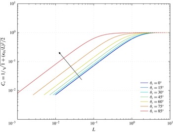
Figure 3 shows the confinement-correction factor
 $C_{c}$
as a function of the dimensionless channel width
 $L$
for different contact angles
 $\unicode[STIX]{x1D703}_{c}$
, and
 $C_{c}$
exhibits small- and large-
 $L$
limiting behaviours clearly. In the small-
 $L$
limit, a more confined pool (smaller
 $L$
) yields a meniscus with a smaller
 $C_{c}$
at a given
 $\unicode[STIX]{x1D703}_{c}$
. In the large-
 $L$
limit,
 $C_{c}$
approaches unity, which implies that confinement effects disappear, i.e. equation (2.1) is recovered from (3.16). A detailed examination of these two limits can be found in appendix C.
Confinement-correction factor
 $C_{c}$
as a function of dimensionless channel width
 $L$
. The values are computed from (3.18). The arrow denotes the direction of increasing
 $\unicode[STIX]{x1D703}_{c}$
. The value of
 $C_{c}$
decreases as the liquid wets the container wall, i.e. for lower
 $\unicode[STIX]{x1D703}_{c}$
.

Interestingly, the power-law dependence of
 $C_{c}$
on
 $L$
is independent of
 $\unicode[STIX]{x1D703}_{c}$
at small
 $L$
, and hence
 $\unicode[STIX]{x1D705}_{0}$
depends only on
 $\unicode[STIX]{x1D703}_{c}$
. It is related to the influence of gravity on the meniscus shape and is discussed in § 6.
It is particularly interesting to analyse (3.14) in the small-
 $L$
limit. In this limit,
 $C_{c}\rightarrow L/\sqrt{2}\cos \unicode[STIX]{x1D703}_{c}$
, as explained in § C.1. The resulting equation becomes independent of
 $L$
and exhibits the power-law behaviour
 $O(Ca^{2/3})$
:
 $$\begin{eqnarray}T=\frac{0.9458}{\sqrt{2}\cos \unicode[STIX]{x1D703}_{c}}Ca^{2/3}.\end{eqnarray}$$
Therefore, the prefactor of (3.2) depends only on
 $\unicode[STIX]{x1D703}_{c}$
in the small-
 $L$
limit. When the coating liquid wets the wall almost completely (small
 $\unicode[STIX]{x1D703}_{c}$
), the meniscus is distorted further, and a thinner film is entrained. Similar results can be found in the inclined unconfined dip coating problem (Wilson Reference Wilson1982); the thinner film is located on the side where the meniscus shape is concave.
The matching condition of Landau & Levich (Reference Landau and Levich1942) that yields (3.14) appears to be irrational. However, matched asymptotic expansions show that this condition is valid for
 $Ca^{1/3}\ll 1$
(Wilson Reference Wilson1982; Park & Homsy Reference Park and Homsy1984; Münch Reference Münch2002). Equation (3.14) is equivalent to the leading-order approximation of the asymptotic expansion in
 $Ca^{1/3}$
. Hence, the error behaviour of the equation can be predicted by investigating the previous study of Wilson (Reference Wilson1982), in which unconfined dip coating is discussed. In his study, when the inclination angle
 $\unicode[STIX]{x1D6FC}=0$
(vertical withdrawal),
 $C_{2}$
in (30) corresponds to our
 $C$
in (3.9) and (3.14) becomes the leading-order term of his equation (39). In terms of our characteristic length, the first correction is
 $O(Ca)$
(note that the first correction is
 $O(Ca^{1/2})$
in his study because of the different characteristic length from the present study). Therefore, one might expect the error behaviour of (3.14) to be
 $O(Ca)$
for low
 $Ca$
. However, Wilson (Reference Wilson1982) also discussed the non-uniformity in his asymptotic series that arises from
 $\unicode[STIX]{x1D6FC}$
. We, therefore, can predict the non-uniformity arising from the contact angle
 $\unicode[STIX]{x1D703}_{c}$
, which changes the meniscus profile at the given
 $Ca$
and
 $L$
, in confined dip coating. The error behaviour is briefly discussed in § 5.3.
The approach that leads to (3.14) can also be easily extended to other film-thickness-predicting equations on the basis of the curvature matching for unconfined dip coating such as that of White & Tallmadge (Reference White and Tallmadge1965) and Spiers et al. (Reference Spiers, Subbaraman and Wilkinson1974). See appendix B for details.
4 Channel-controlled regime
At high
 $Ca$
, it is expected that the viscous force transferred from the moving plate is sufficiently large to set the contact line on the stationary wall in motion (i.e. the contact line may move upwards along the wall) as with the forced wetting (Blake & Ruschak Reference Blake and Ruschak1979); there is no steady-state flow as long as the contact line moves. However, the contact line would eventually cease to move and be pinned on a wall that has received special treatments such as an application of surface roughening or at the sharp corner of a wall that the moving contact line reaches (Oliver, Huh & Mason Reference Oliver, Huh and Mason1977), as shown in figure 1(b). In what follows, we consider a steady-state flow with the pinned contact line.
4.1 Limiting behaviour of film thickness in channel-controlled regime
The flow in the channel region is fully developed, as mentioned in § 2, and hence the Stokes equations with boundary conditions (2.27)–(2.30) can be greatly simplified to give a velocity field
 $$\begin{eqnarray}u=1+\frac{1}{2}\left(\frac{L^{2}}{Ca}+\frac{\text{d}^{}p_{c}}{\text{d}^{}x}\right)(y^{2}-y)-y.\end{eqnarray}$$
We can obtain the flow rate in units of
 $u_{s}\,l$
through the channel from the velocity field:
 $$\begin{eqnarray}q_{c}=\frac{1}{2}-\frac{1}{12}\frac{\text{d}}{\text{d}x}(p_{c}+G_{c}x).\end{eqnarray}$$
The flow rate
 $q_{c}$
should be equal to that through the film entrainment region. It has been given by Van Rossum (Reference Van Rossum1958) as
 $$\begin{eqnarray}q_{f}=T\left(1-{\textstyle \frac{1}{3}}G_{c}T^{2}\right).\end{eqnarray}$$
The term involving
 $G_{c}$
represents the gravitational drainage in the film entrainment region. The drainage is negligible at high
 $Ca$
 $\gg L^{2}$
because
 $G_{c}T^{2}<L^{2}/Ca$
in confined dip coating, where the film thickness is expected to be smaller than the channel width; i.e.
 $T<1$
. Therefore, the dimensionless thickness
 $T$
is given by
 $$\begin{eqnarray}T=\frac{1}{2}-\frac{1}{12}\frac{\text{d}^{}p_{c}}{\text{d}^{}x}.\end{eqnarray}$$
This result means that
 $T$
can be determined by considering only the pressure gradient inside the channel.
Besides, the flow inside the channel at high
 $Ca$
resembles the coating flow under a knife or blade. The well-developed theory for knife coatings shows that the film thickness is half the coating gap for a blade parallel to a moving plate under negligible surface tension (Ruschak Reference Ruschak1985; Coyle Reference Coyle1997). Here, the gap is the distance between the moving plate and the blade face, which is essentially identical to the channel width
 $l$
in confined dip coating. We can therefore expect that
 $\text{d}p_{c}/\text{d}x$
will eventually vanish in the high-
 $Ca$
limit, from knife coating theory. As a result, the flow becomes an almost pure Couette flow, and
 $T$
tends to
 $1/2$
when
 $Ca$
approaches infinity:
 $$\begin{eqnarray}T\rightarrow {\textstyle \frac{1}{2}}\quad \text{as}\;Ca\rightarrow \infty .\end{eqnarray}$$
This result appears to be similar to that of unconfined dip coating:
 $h_{\infty }^{\ast }/l_{f}$
becomes independent of
 $Ca$
in the high-
 $Ca$
limit in the absence of inertia and surfactants (Esmail & Hummel Reference Esmail and Hummel1975b
; Weinstein & Ruschak Reference Weinstein and Ruschak2001; Jin et al.
Reference Jin, Acrivos and Münch2005). However, the film thickness
 $h_{\infty }^{\ast }$
itself increases without bound with
 $Ca$
in unconfined dip coating, whereas
 $h_{\infty }^{\ast }$
is bounded in confined dip coating.
5 Numerical computations
5.1 Finite element model
To solve the Stokes equations with the Galerkin finite element method (G/FEM), we need more boundary conditions, in addition to conditions (2.6)–(2.9). These boundary conditions are represented in the following.
A stationary wall with the no-slip condition should be included in the analysis to incorporate the confinement effects. Such a wall can be found in early numerical models for unconfined dip coating (Jenny & Souhar Reference Jenny and Souhar2009; Filali et al. Reference Filali, Khezzar and Mitsoulis2013); however, there is also an inlet feed port to compensate for the mass loss at the outflow boundary in those models. The reliability of a numerical model with such an inlet feed would depend on the location of the feed; the flow through a feed that is not far enough from the meniscus affects the film thickness when a pool is confined. Besides, the numerical models with sufficient distance between the meniscus and the feed may be more computationally expensive than our FE model explained in the following.
The meniscus contacts the stationary wall at an angle
 $\unicode[STIX]{x1D703}_{}$
on the contact line:
 $$\begin{eqnarray}\boldsymbol{n}_{m}\boldsymbol{\cdot }\boldsymbol{n}_{w}=-\cos \unicode[STIX]{x1D703}_{},\end{eqnarray}$$
where
 $\boldsymbol{n}_{m}$
and
 $\boldsymbol{n}_{w}$
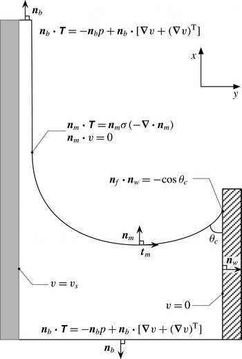
are the outward normal unit vectors on the meniscus and the wall, respectively. The definitions of the normal and tangent vectors and a contact angle in our FE model are shown in figure 4. When the coating liquid near the stationary wall remains in static equilibrium, the static contact angle
 $\unicode[STIX]{x1D703}_{c}$
is used instead of
 $\unicode[STIX]{x1D703}_{}$
.
Numerical flow domain and corresponding boundary conditions. All boundary conditions, unit vectors and a contact angle are represented. The free boundary condition is applied to both the inflow (bottom) and outflow (top) boundaries. The velocity profile is not prescribed.

Dip coating is a self-metered method in that the flow rate is determined by the force balance inside the coating flow (Weinstein & Ruschak Reference Weinstein and Ruschak2001). Therefore, a velocity profile should not be prescribed at the inflow or outflow boundary a priori; such a prescribed velocity profile presets the film thickness
 $h_{\infty }^{\ast }$
.
In this regard, the FEM has an advantage over other methods, because of the free boundary condition (Papanastasiou, Malamataris & Ellwood Reference Papanastasiou, Malamataris and Ellwood1992). The FEM can extend the validity of the weak form of the governing equations to synthetic boundaries (inflow and outflow boundaries), instead of replacing them with unknown essential or natural boundary conditions, such that
 $$\begin{eqnarray}\boldsymbol{n}_{b}\boldsymbol{\cdot }\unicode[STIX]{x1D64F}^{\ast }=-\boldsymbol{n}_{b}\,p^{\ast }+\boldsymbol{n}_{b}\boldsymbol{\cdot }\unicode[STIX]{x1D707}[\unicode[STIX]{x1D735}^{\ast }\boldsymbol{v}^{\ast }+(\unicode[STIX]{x1D735}^{\ast }\boldsymbol{v}^{\ast })^{\text{T}}],\end{eqnarray}$$
where
 $\boldsymbol{n}_{b}$
is the outward unit normal vector at either the inflow or outflow boundary. The free boundary condition (5.2), which is typically used for an outflow boundary, appears not to impose any boundary condition at all; however, it provides an effective boundary condition (Renardy Reference Renardy1997).
We apply the free boundary condition (5.2) not only to the outflow boundary but also to the inflow boundary. To the best of the authors’ knowledge, this has never been attempted before. In our FE model, both the inflow and outflow boundaries are located sufficiently far from each other so that the velocity fields and the gradient of the pressure fields are expected to approach asymptotic limits at both ends. This asymptotic state includes ‘fully developed’ flows (Renardy Reference Renardy1997). Applying the free boundary condition to the inflow boundary allows the pressure to take any value at the boundary. It yields the undetermined position of the contact line with the contact angle prescribed by (5.1). However, at a given
 $Ca$
and
 $L$
, both the position of the contact line and the contact angle should be fixed to have a unique solution in the frame of reference for our model, but it is impossible to impose them as boundary conditions in our FE framework simultaneously. Therefore, an additional condition or constraint is required to find the unique solution. It would seem that the mesh configuration of the physical domain of interest provides the additional condition required to determine the position of the contact line implicitly. When the mesh generation equation (explained in the following) is solved with (2.4) and (2.5) simultaneously, we can find the unique (steady-state) solution. However, the detailed mechanism of how the mesh configuration fixes the position of the contact line is not clear.
As discussed earlier, the physical domain of interest of the confined dip coating flow should be surrounded by three physical boundaries (the meniscus, the stationary wall and the moving plate) and two synthetic boundaries (the inflow and outflow planes). All the boundary conditions are summarised in figure 4.
To find the meniscus shape via standard techniques for boundary value problems, the set of differential equations and boundary conditions on the unknown, deformable ‘physical’ region
 $R$
in the
 $x^{\ast }y^{\ast }$
-plane should be transformed one to one into an equivalent set on the known, fixed ‘computational’ region
 $G$
in the
 $\unicode[STIX]{x1D709}\unicode[STIX]{x1D702}$
-plane. Here
 $R$
and the set on it are transformed by an equation of the form
 $\boldsymbol{x}^{\ast }=\boldsymbol{M}(\unicode[STIX]{x1D743})$
, where
 $\boldsymbol{x}^{\ast }=(x^{\ast },y^{\ast })$
and
 $\unicode[STIX]{x1D743}=(\unicode[STIX]{x1D709},\unicode[STIX]{x1D702})$
. Any function
 $f(\boldsymbol{x}^{\ast })$
defined on
 $R$
can be thought of as a function
 $f(\boldsymbol{x}^{\ast }(\unicode[STIX]{x1D743}))$
defined on
 $G$
as well. The image
 $\unicode[STIX]{x1D743}$
of
 $\boldsymbol{x}^{\ast }$
under the inverse transformation
 $\boldsymbol{M}^{-1}$
is a solution to elliptic partial differential equations, which is similar to that for the diffusional mass transport for the dilute regime,
 $$\begin{eqnarray}\unicode[STIX]{x1D735}^{\ast }\boldsymbol{\cdot }(D_{\unicode[STIX]{x1D709}}\unicode[STIX]{x1D735}^{\ast }\unicode[STIX]{x1D709})=0,\quad \unicode[STIX]{x1D735}^{\ast }\boldsymbol{\cdot }(D_{\unicode[STIX]{x1D702}}\unicode[STIX]{x1D735}^{\ast }\unicode[STIX]{x1D702})=0,\end{eqnarray}$$
where
 $D_{\unicode[STIX]{x1D709}}$
and
 $D_{\unicode[STIX]{x1D702}}$
are mesh diffusivities, which determine the gradients of the coordinate potentials
 $\unicode[STIX]{x1D709}$
and
 $\unicode[STIX]{x1D702}$
adjusting the nodal distribution inside the ‘physical’ region
 $R$
. The nodal distribution at the boundaries, prescribed by the functions defining their geometries, is specified by a stretching function (Vinokur Reference Vinokur1983). The iso-contour curves of
 $\unicode[STIX]{x1D709}$
and
 $\unicode[STIX]{x1D702}$
define the boundaries of the quadrilateral elements used to tessellate
 $R$
, and the intersection points of these curves determine the nodal positions. The meniscus shape is implicitly determined by the kinematic condition (2.8). Equations (5.3) have been called the elliptic mesh generation equations, and they have been discussed in detail by de Santos (Reference de Santos1991).
5.2 Solution using the finite element model
The field variables, such as the velocity, pressure and nodal position, are approximated by a linear combination of the polynomial basis functions. The velocity and nodal position are approximated by a Lagrangian biquadratic function
 $\unicode[STIX]{x1D719}_{i}^{}(\unicode[STIX]{x1D709},\unicode[STIX]{x1D702})$
, and the pressure is approximated by a linear discontinuous function
 $\unicode[STIX]{x1D713}_{k}^{}(\unicode[STIX]{x1D709},\unicode[STIX]{x1D702})$
:
 $$\begin{eqnarray}\boldsymbol{x}^{\ast }=\mathop{\sum }_{i=1}^{n}\boldsymbol{x}_{i}^{\ast }\unicode[STIX]{x1D719}_{i}^{}(\unicode[STIX]{x1D709},\unicode[STIX]{x1D702}),\quad \boldsymbol{v}^{\ast }=\mathop{\sum }_{i=1}^{n}\boldsymbol{v}_{i}^{\ast }\unicode[STIX]{x1D719}_{i}^{}(\unicode[STIX]{x1D709},\unicode[STIX]{x1D702}),\quad p^{\ast }=\mathop{\sum }_{i=1}^{m}p_{i}^{\ast }\unicode[STIX]{x1D713}_{i}^{}(\unicode[STIX]{x1D709},\unicode[STIX]{x1D702}),\end{eqnarray}$$
where
 $n$
is the number of nodes used for the nodal position and velocity and
 $m$
is the number of nodes used for the pressure, and the coefficients
 $\boldsymbol{x}_{i}^{\ast }$
,
 $\boldsymbol{v}_{i}^{\ast }$
and
 $p_{i}^{\ast }$
are unknown values to be determined at each node.
The weak forms of (2.4), (2.5) and (5.3) are obtained by multiplying them by the weighting functions and then integrating over the ‘physical’ region
 $R$
. The essential boundary conditions are implemented by replacing the corresponding weighted residual equation with the desired velocity or node specification. The natural boundary conditions are implemented through the boundary integrals, which follow from the divergence theorem. Note that the free boundary condition (5.2) is treated as the natural boundary condition.
The G/FEM reduces the Stokes and mesh generation equations (2.4), (2.5) and (5.3) to a set of nonlinear algebraic equations with respect to the basis function coefficients,
 $$\begin{eqnarray}\boldsymbol{R}(\boldsymbol{z},\unicode[STIX]{x1D740})=\mathbf{0},\end{eqnarray}$$
where
 $\boldsymbol{z}$
is the solution vector consisting of the FE coefficients of
 $\boldsymbol{x}_{i}^{\ast }$
,
 $\boldsymbol{v}_{i}^{\ast }$
and
 $p_{i}^{\ast }$
; and
 $\unicode[STIX]{x1D740}$
is the parameter vector containing the parameters for the dip coating flow, such as
 $l$
,
 $u_{s}$
,
 $\unicode[STIX]{x1D703}_{c}$
,
 $\unicode[STIX]{x1D70C}$
and
 $\unicode[STIX]{x1D70E}$
. The system of nonlinear equations (5.5) is solved using Newton’s method:
 $$\begin{eqnarray}\left.\begin{array}{@{}c@{}}\unicode[STIX]{x1D645}_{\boldsymbol{R}}(\boldsymbol{z}^{i}|\unicode[STIX]{x1D740})\unicode[STIX]{x1D6FF}\boldsymbol{z}^{i}=-\boldsymbol{R}(\boldsymbol{z}^{i},\unicode[STIX]{x1D740}),\\ \boldsymbol{z}^{i+1}=\boldsymbol{z}^{i}+\unicode[STIX]{x1D6FF}\boldsymbol{z}^{i},\end{array}\right\}\end{eqnarray}$$
where
 $\unicode[STIX]{x1D645}_{\boldsymbol{R}}(\boldsymbol{z})$
is the Jacobian matrix of
 $\boldsymbol{R}$
. The solution vector
 $\boldsymbol{z}$
is accepted as the solution to the problem when
 $\Vert \boldsymbol{R}(\boldsymbol{z}^{i})\Vert _{2}<5\times 10^{-9}$
. The typical value of the solution update
 $\Vert \unicode[STIX]{x1D6FF}\boldsymbol{z}^{i}\Vert _{2}$
is of the order of
 $10^{-5}$
at convergence.
We use a direct numerical solver based on the frontal algorithm (Duff, Erisman & Reid Reference Duff, Erisman and Reid1989). It appears that there is no zero pivot during the matrix decomposition step; thus, we can safely conclude that the free boundary condition (5.2) at both the inflow and outflow boundaries does not yield an ill-posed problem in the resulting discrete-level matrix system (5.6).
The initial guess was obtained by replacing the unknown meniscus shape with a known arc of a circle and substituting the stress balance condition (2.8) with the kinematic condition (2.9) and Navier’s slip condition with a large slip coefficient
 $\unicode[STIX]{x1D6FD}=10^{8}$
along the meniscus,
 $\unicode[STIX]{x1D6FD}(\boldsymbol{t}_{m}\boldsymbol{n}_{m}\boldsymbol{ : }\unicode[STIX]{x1D64F}^{\ast })=\boldsymbol{t}_{m}\boldsymbol{\cdot }\boldsymbol{v}^{\ast }$
. Nodal positions were not included in the unknowns because the normal and tangential unit vectors at the meniscus were known at this stage; Navier’s slip condition and the kinematic condition (2.9) were applied to the
 $x^{\ast }$
- and
 $y^{\ast }$
-components of the momentum equation (2.5), respectively. The base solution at
 $Ca=0.01$
,
 $L=5$
and
 $\unicode[STIX]{x1D703}_{c}=30^{\circ }$
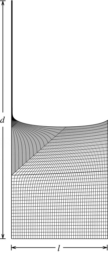
was computed using the initial guess. Figure 5 illustrates the mesh configuration of the base solution. Along the meniscus, a total of 125 elements and 251 nodes were used to resolve the meniscus shape.
Mesh configuration at
 $Ca=0.01$
,
 $L=5$
and
 $\unicode[STIX]{x1D703}_{c}=30^{\circ }$
. 2775 quadrilateral elements are tessellated into the physical domain. A total of 125 elements and 251 nodes is used to resolve the curved meniscus shape. The aspect ratio of the mesh configuration is adjusted for visualisation (
 $d=6\,l$
).

The solutions for different values of the capillary number
 $Ca$
and the dimensionless channel width
 $L$
were computed by using the pseudo-arc-length continuation (Bolstad & Keller Reference Bolstad and Keller1986), starting from the base solution.
 $u_{s}$
and
 $l$
were chosen as the continuation parameters to adjust
 $Ca$
and
 $L$
, respectively. During the continuation in
 $l$
, the distance
 $d$
between the inflow and outflow boundaries should be adjusted simultaneously to ensure a fully developed flow at the inflow and outflow boundaries. When the inflow is not fully developed, the accuracy of the flow rate through the flow domain could be compromised, and hence the film thickness
 $h_{\infty }^{\ast }$
. Unlike other numerical models (Jin et al.
Reference Jin, Acrivos and Münch2005; Campana et al.
Reference Campana, Ubal, Giavedoni and Saita2013), we did not restrict the shape of the free surface at the corner of the element where the outflow boundary and the free surface are placed. Hence, the free surface slope with respect to the moving plate is a major indicator of fully developed flow. When the outflow is not fully developed, the thickness being measured from the moving plate to the free surface along the outflow boundary is larger than the film thickness
 $h_{\infty }^{\ast }$
. According to our numerical tests, it turns out that
 $d/l=6$
ensures a virtually parabolic velocity profile and a zero slope of the free surface at the corner at the outflow boundary. We therefore maintained
 $d/l=6$
during the continuation.
Steady-state solutions are obtained within 3–5 iterations except for the base solution obtained using the initial guess. To guarantee a high accuracy for
 $h_{\infty }^{\ast }$
, we verified that the mesh configuration near the highly curved meniscus is properly resolved for every solution.
5.3 Numerical results
We validated our FE model by comparison with results from other models and experiments on unconfined dip coating. See appendix D for details.
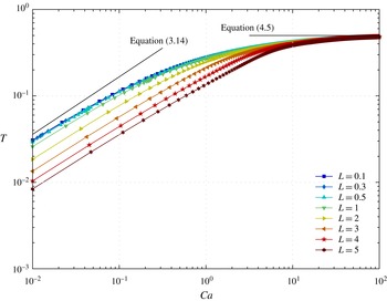
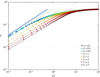
The results of the FE computations confirm that (3.20) and (4.5) represent the meniscus- and channel-controlled regimes, respectively. The curves computed at the dimensionless channel width
 $L<0.5$
overlap and are virtually indistinguishable, as shown in figure 6. The overlapped curve exhibits power-law dependence and is independent of
 $L$
in the low-
 $Ca$
regime. This dependence is already predicted by (3.20).
Dimensionless film thickness
 $T$
versus capillary number
 $Ca$
for
 $\unicode[STIX]{x1D703}_{c}=30^{\circ }$
and various
 $L$
. The curves of
 $T$
overlap at
 $L<0.5$
.

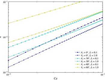
Figure 7 shows the difference between the analytical and numerical results. Interestingly, the error behaviours are distinct at different contact angles. The error follows a power-law behaviour
 $\unicode[STIX]{x1D716}=O(Ca^{m})$
, where
 $m$
is unity for
 $\unicode[STIX]{x1D703}_{c}=30^{\circ }$
, but changes to
 $m\simeq 0.75$
for
 $\unicode[STIX]{x1D703}_{c}=60^{\circ }$
. This distinction appears to be due to the non-uniformity mentioned in § 3.1. A full asymptotic analysis is required to investigate the non-uniformity; however, it is beyond the scope of the present study.
Error
 $\unicode[STIX]{x1D716}$
behaviour. The error is defined as the difference between the analytical and numerical results. The dimensionless film thickness
 $T$
is predicted by (3.14) and (3.20) for
 $L=1$
and
 $L=0.1$
, respectively. The plot shows the errors of
 $O(Ca)$
at
 $\unicode[STIX]{x1D703}_{c}=30^{\circ }$
and
 $O(Ca^{4/3})$
at
 $\unicode[STIX]{x1D703}_{c}=0^{\circ }$
, as indicated by Wilson (Reference Wilson1982) and Park & Homsy (Reference Park and Homsy1984), respectively.

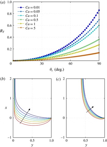
Figure 8 shows the effect of the contact angle
 $\unicode[STIX]{x1D703}_{c}$
on the dimensionless thickness
 $T$
.
 $T$
increases with
 $\unicode[STIX]{x1D703}_{c}$
as can be seen in (3.20). However, the dependence of
 $T$
on
 $\unicode[STIX]{x1D703}_{c}$
decreases as
 $Ca$
increases, as shown in figure 8(a). This is because the meniscus shape becomes less sensitive to
 $\unicode[STIX]{x1D703}_{c}$
for high
 $Ca$
, as can be seen from a comparison of figures 8(b) (
 $Ca=0.01$
) and (c) (
 $Ca=5$
). The results clearly show that the capillary effect is crucial in the meniscus-controlled regime discussed in § 3, and the pressure gradient inside the channel region is crucial in the channel-controlled regime discussed in § 4.
Influence of container wall wetting on film thickness and meniscus shape for
 $L=0.1$
and various
 $Ca$
. (a) Plot of
 $R_{T}\equiv (T-T_{0})/T_{0}$
, where
 $T_{0}$
is the value at
 $\unicode[STIX]{x1D703}_{c}=0$
. The effect of the wall wetting on the film thickness diminishes as
 $Ca$
increases. (b,c) The coordinates are scaled with
 $l$
. The arrows denote the direction of increasing
 $\unicode[STIX]{x1D703}_{c}$
. The meniscus shape changes significantly for
 $Ca=0.01$
, whereas it changes slightly for
 $Ca=5$
.

In the high-
 $Ca$
regime, the pressure gradient
 $\text{d}p_{c}/\text{d}x$
at the inflow boundary and the gravity
 $G_{c}$
monotonically decrease as
 $Ca$
increases, but
 $G_{c}$
decreases faster than
 $\text{d}p_{c}/\text{d}x$
(
 $G_{c}=o(\text{d}p_{c}/\text{d}x)$
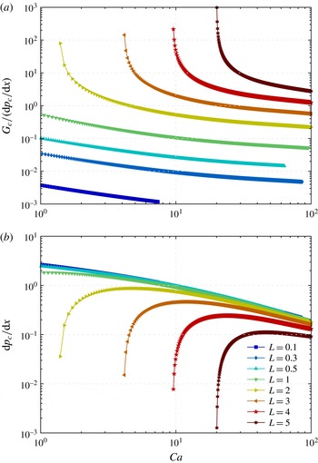
), as shown in figure 9(a). Note that
 $\text{d}p_{c}/\text{d}x$
does not rapidly vanish as
 $Ca$
increases, as shown in figure 9(b). However, we can expect that
 $\text{d}p_{c}/\text{d}x$
will vanish eventually in the high-
 $Ca$
limit, and the flow will become a Couette flow (see appendix A for details). The numerical results are consistent with the discussion in § 4.1. Interestingly,
 $\text{d}p_{c}/\text{d}x$
is independent of
 $L$
at small
 $L$
(
 ${<}0.5$
) for high
 $Ca$
, as shown in figure 9(b), and hence
 $T$
is also independent of
 $L$
. This independence is identical to that found in the low-
 $Ca$
regime with small
 $L$
. Finally, all the numerical results show that
 $l$
is the critical parameter for both regimes.
(a) The ratio of gravitational force
 $G_{c}$
to pressure force
 $\text{d}p_{c}/\text{d}x$
and (b)
 $\text{d}p_{c}/\text{d}x$
as a function of capillary number
 $Ca$
for different
 $L$
at
 $\unicode[STIX]{x1D703}_{c}=30^{\circ }$
. (a)
 $G_{c}$
decays faster than
 $\text{d}p_{c}/\text{d}x$
as
 $Ca$
increases. (b) When the pool is sufficiently confined (
 $L<0.5$
),
 $\text{d}p_{c}/\text{d}x$
becomes independent of
 $L$
. Although
 $\text{d}p_{c}/\text{d}x$
does not vanish completely, even at an extremely high
 $Ca$
of up to
 $10^{2}$
, it clearly decreases monotonically.

6 Characteristic length transition: vanishing gravitational effect
In confined dip coating, the dimensionless thickness
 $T$
becomes independent of the dimensionless channel width
 $L$
for two limit cases: low
 $Ca$
(meniscus-controlled regime with small
 $L$
, § 3), and high
 $Ca\gg L^{2}$
(channel-controlled regime, § 4). For both limit cases, the gravitational force is overwhelmed by either the capillary or the viscous force. A comparison of gravity with the surface tension or viscous drag can aid understanding of these limits.
In the meniscus-controlled regime, the local relative importance of the gravitational and capillary forces in the dynamic meniscus region can be measured by
 $\unicode[STIX]{x1D70C}gh^{\ast }/(\unicode[STIX]{x1D70E}/l)$
. However, we utilise a more relevant quantity, defined in (2.19):
 $$\begin{eqnarray}G_{d}\equiv Ca^{1/3}L^{2}.\end{eqnarray}$$
Note that
 $G_{d}$
is an upper bound of
 $\unicode[STIX]{x1D70C}gh^{\ast }/(\unicode[STIX]{x1D70E}/l)$
.
 $G_{d}$
vanishes when the channel is confined further (
 $L<0.5$
), which reinforces the capillary force due to the highly curved meniscus. For small
 $L$
, gravity is negligible in the Stokes equations (2.15) and (2.22), and
 $T$
becomes independent of
 $L$
as shown in (3.20). This means that the effect of gravity diminishes not only in the dynamic meniscus region but also in the static meniscus region. It is already signalled in
 $\unicode[STIX]{x1D705}_{0}$
. For low
 $L$
,
 $\unicode[STIX]{x1D705}_{0}$
depends only on
 $\unicode[STIX]{x1D703}_{c}$
as mentioned in § 3.1 and becomes
 $\unicode[STIX]{x1D705}_{0}=2\cos \unicode[STIX]{x1D703}_{c}$
; therefore, the meniscus shape becomes an arc of a circle in the low-
 $Ca$
limit.
The resulting Stokes equations (without gravity) can also be found in the Bretherton problem in Hele-Shaw cells, where gravity is also insignificant (Park & Homsy Reference Park and Homsy1984). Furthermore, equation (3.20) with a zero contact angle becomes the leading-order approximation for the problem. Note that this contact angle stands for a two-sided coating on the walls of the cells. The Bretherton problem in Hele-Shaw cells, therefore, can be regarded as the limiting case of the confined dip coating problem, and the error behaviour is consistent with
 $O(Ca^{4/3})$
as indicated by Park & Homsy (Reference Park and Homsy1984), as shown in figure 7. See appendix E for a comparison between confined dip coating and the Bretherton problems.
In the channel-controlled regime, similar to the meniscus-controlled regime, the competition between the gravitational and viscous forces can be measured by
 $$\begin{eqnarray}G_{c}\equiv \frac{L^{2}}{Ca}=\frac{\unicode[STIX]{x1D70C}gl}{\unicode[STIX]{x1D707}u_{s}/l}.\end{eqnarray}$$
 $G_{c}$
vanishes when the plate withdraws rapidly or when the channel is highly confined (
 $Ca\gg L^{2}$
), which enhances the viscous force inside the channel. In the high-
 $Ca$
limit,
 $T$
becomes independent of
 $L$
. This corresponds to the vanishing of the gravitational effect.
The independence of
 $T$
from
 $L$
for both low- and high-
 $Ca$
regimes reveals a change in the number of dimensionless numbers required to describe the confined dip coating flow uniquely. As discussed in § 2.1, for withdrawal of a flat substrate from a pool of a pure Newtonian fluid, unconfined dip coating flows require three dimensionless numbers (or two for inertialess flows:
 $h_{\infty }^{\ast }/l_{c}$
and
 $Ca$
). Adding the channel width
 $l$
to the dimensional analysis increases the number of dimensionless numbers to four (or three for inertialess flows:
 $T$
,
 $Ca$
and
 $L$
). However, when the gravitational effect vanishes, the number becomes three again (or two for inertialess flows:
 $T$
and
 $Ca$
). Note that the definitions of
 $T$
and
 $Ca$
are independent of
 $g$
. According to the FE computations, these vanishing gravitational effects occur over the entire range of
 $Ca$
when
 $L$
is sufficiently small; e.g.
 $L<0.5$
according to our numerical results, as shown in figure 6.
The change in the number of dimensionless numbers for the system implies a transition of the system’s characteristic length. The length of the unconfined pool is the capillary length
 $l_{c}$
. When the pool is confined, the newly introduced
 $l$
competes with
 $l_{c}$
, and this competition is parameterised by
 $L=l/l_{c}$
. When the gravitational effect vanishes,
 $l_{c}$
is no longer effective, and
 $l$
becomes the only characteristic length for confined dip coating flows.
7 Concluding remarks
The unconfined pool assumption is valid only in the absence of a stationary wall influencing the film thickness
 $h_{\infty }^{\ast }$
. In such a pool,
 $h_{\infty }^{\ast }$
should be independent of the channel width
 $l$
; i.e.
 $T$
is inversely proportional to
 $L$
, regardless of
 $Ca$
. This criterion for an unconfined pool can be expressed as
 $$\begin{eqnarray}\frac{\unicode[STIX]{x2202}(LT)}{\unicode[STIX]{x2202}L}=0.\end{eqnarray}$$
Otherwise, a pool is confined. It should be emphasised that the pool can be confined either via small
 $L$
or via high
 $Ca$
, and hence it is possible for an unconfined pool to become confined as
 $Ca$
increases. In a confined pool,
 $l$
becomes the appropriate characteristic length of the system, and two major changes occur: an increase in the curvature of the meniscus and an intensification in the viscous stress inside the channel. The increased curvature enhances the capillarity and affects the force balance in the dynamic meniscus region. The intensified viscous stress dominates the (dimensional) pressure gradient in the channel region. These changes affect the flow rate and hence the film thickness
 $h_{\infty }^{\ast }$
, and we call them the confinement effects in dip coating.
In confined dip coating, the role of gravity in the force balance diminishes when
 $Ca^{1/3}\ll 1$
and
 $L<0.5$
; or
 $Ca\gg L^{2}$
. Consequently, the characteristic length is no longer determined by the material properties but by the channel width
 $l$
. The confinement effects for a dip coating flow are strongly associated with the vanishing gravitational effect and the increasing importance of the newly introduced characteristic length
 $l$
.
The dynamic and channel regions are important as they determine the flow rate and hence the film thickness at low and high
 $Ca$
, respectively. The thickness-determining mechanisms in each region correspond to the two regimes of confined dip coating flows, i.e. the meniscus- and channel-controlled regimes. The criteria for both regimes cannot be explicitly determined because the threshold
 $Ca$
of both regimes depends on the dimensionless channel width
 $L$
, as shown in figure 6. However, when the gravitational effect vanishes (
 $L<0.5$
), the ranges of
 $Ca\lesssim 0.1$
and
 $Ca\gtrsim 10$
can be established for the meniscus- and channel-controlled regimes, respectively.
Between the two regimes, there is a regime where the normal viscous stress becomes comparable with the capillary pressure in the dynamic meniscus region. This regime was also observed in unconfined dip coating (Esmail & Hummel Reference Esmail and Hummel1975a
; Jin et al.
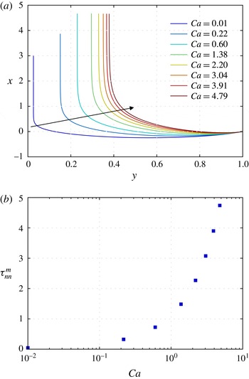
Reference Jin, Acrivos and Münch2005). The meniscus shape changes abruptly in the dynamic meniscus region for low
 $Ca$
, but the magnitude of the change diminishes as
 $Ca$
increases, as shown in figure 10(a). For high
 $Ca>1$
, the shape does not change significantly, and hence the capillary pressure jump. In contrast, the normal viscous stress increases monotonically and dominates the capillary pressure, as shown in figure 10(b). In this regime, the flow is no longer unidirectional, and the strong acceleration along the meniscus generates a non-negligible normal viscous stress in the dynamic meniscus region. Under these conditions, lubrication-type simple models cannot be used, and a nonlinear two-dimensional model must be employed to determine the meniscus shape (Esmail & Hummel Reference Esmail and Hummel1975b
). Analysis of this regime is beyond the scope of the present study but merits further discussion.
Meniscus shape change and maximum normal viscous stress for
 $L=1$
and
 $\unicode[STIX]{x1D703}_{c}=30^{\circ }$
. (a) The coordinates are in units of
 $l$
. The arrow denotes the direction of increasing
 $Ca$
. The meniscus shape changes abruptly in the dynamic meniscus region for low
 $Ca$
, but this change diminishes with increasing
 $Ca$
. (b)
 $\unicode[STIX]{x1D70F}_{nn}^{m}$
is the maximum magnitude of the normal viscous stress on the meniscus.
 $\unicode[STIX]{x1D70F}_{nn}^{m}$
is expressed in units of capillary pressure based on the meniscus shape, which is an arc of a circle with a contact angle of
 $30^{\circ }$
at the wall.
 $\unicode[STIX]{x1D70F}_{nn}^{m}$
increases monotonically with
 $Ca$
. It should be mentioned that the numerical results obtained with quadratic basis functions for the velocity and position variables yield wiggles in the profile of the normal viscous stress on the meniscus. Therefore, the result for the magnitude of
 $\unicode[STIX]{x1D70F}_{nn}^{m}$
may be less accurate than those for other primitive variables, such as the position and velocity.

Inertia was not considered in the present study. The importance of inertia depends on the material number
 $m$
. The inertia begins to surpass the surface tension at a Weber number (
 $We=ReCa$
) close to unity and becomes comparable to the viscous drag (Campana et al.
Reference Campana, Ubal, Giavedoni and Saita2013). For unconfined dip coating, thickening or thinning of the film occurs above a threshold value of
 $Ca$
at large
 $Re$
and low
 $Ca$
(Tallmadge & Stella Reference Tallmadge and Stella1968; de Ryck & Quéré Reference de Ryck and Quéré1998) or at large
 $Re$
and high
 $Ca$
(Esmail & Hummel Reference Esmail and Hummel1975b
), respectively. In both cases, the maximum thickness scaled with
 $l_{f}$
exists. Besides, the meniscus shape in the dynamic meniscus region becomes wavy, and the coating flow becomes unstable (Esmail & Hummel Reference Esmail and Hummel1975b
; Kamotani, Ostrach & Kizito Reference Kamotani, Ostrach and Kizito1999; Jin et al.
Reference Jin, Acrivos and Münch2005). On the basis of these results, it is expected that thickening or thinning of the film can also occur in confined dip coating with inertia, depending on
 $Re$
(or
 $m$
) and
 $Ca$
. However, the maximum thickness occurs at a lower
 $Ca$
than that in unconfined dip coating, because the narrow channel causes further acceleration of the flow near the meniscus at the same
 $Ca$
. Furthermore, the waviness of the meniscus shape and hence the instability of the meniscus are also expected to be suppressed, because of the presence of the stationary container wall. This regime remains to be analysed.
It is important to mention the non-uniqueness of the film thickness. Wilson (Reference Wilson1982) discussed the possibility of multiple uniform film thicknesses in the non-vertical dip coating problem where the inclination angle (from the vertical) is larger than a critical value. Hocking (Reference Hocking2001) explained that this non-uniqueness arises, at a low capillary number
 $Ca$
, from the presence of the three-phase contact line. Münch & Evans (Reference Münch and Evans2005) and Jin et al. (Reference Jin, Acrivos and Münch2005) investigated the non-uniqueness of the film thickness and the meniscus shape systematically by studying the phase space of an ordinary differential equation for the shape. Furthermore, Münch & Evans (Reference Münch and Evans2006) examined the interaction between the meniscus and the advancing front in the context of Marangoni-driven films. In the dip coating problem, multiple solutions were observed experimentally (Snoeijer et al.
Reference Snoeijer, Delon, Fermigier and Andreotti2006, Reference Snoeijer, Ziegler, Andreotti, Fermigier and Eggers2008), calculated asymptotically (Benilov et al.
Reference Benilov, Chapman, Mcleod, Ockendon and Zubkov2010) and computed numerically (Gao et al.
Reference Gao, Li, Feng, Ding and Lu2016).
The present study is limited to complete wetting of the moving plate by the coating liquid, so that the three-phase contact line at the front of the entrained film is meaningless from the standpoint of thickness determination. In confined dip coating, the film thickness
 $h_{\infty }^{\ast }$
for complete wetting is uniquely determined and is thinner than that in unconfined dip coating. However, for partial wetting, the deposited film exhibits complex behaviour; a thick film in comparison with the film for complete wetting can appear at the front of the entrained film in unconfined dip coating. Snoeijer et al. (Reference Snoeijer, Delon, Fermigier and Andreotti2006) and Gao et al. (Reference Gao, Li, Feng, Ding and Lu2016) showed experimental evidence and numerical predictions regarding the appearance of the thick film, respectively. They also reported that the thickness of the thick film is determined solely by the physics of the three-phase contact line; therefore, we speculate that the thick film would not be significantly affected in confined dip coating.
In the present study, there is no restriction on the liquid supply to the channel. Therefore, the meniscus reaches a steady state and fixes to the wall. Note that, if the liquid supply is limited or is unable to keep pace with the removal by the entrained film, the meniscus cannot be fixed to the wall. In the meniscus-controlled regime, the meniscus recedes with constant velocity, which is a function of the size of the container and the flow rate. In the channel-controlled regime, the solution cannot reach a steady state; the pinned meniscus eventually invades the channel along the wall. It is very similar to the low-flow limit phenomena induced by a limited supply of liquid in slot coating flows (Carvalho & Kheshgi Reference Carvalho and Kheshgi2006). They are signalled by an invasion of the channel between the coating die and the moving plate by the downstream meniscus.
Acknowledgements
This research was supported by the Basic Science Research Program (NRF-2016R1D1A1B03931632) and by the Global Frontier R&D Program of the Center for Multiscale Energy Systems (2012M3A6A7054861) funded by the National Research Foundation of Korea (NRF) under the Ministry of Science, ICT and Future Planning, Korea.
Comparison of FE computation results with previously reported values. For the FE model, the liquid pool is sufficiently large (
 $L=70$
) that the film thickness is unaffected by
 $L$
. The solid line represents the prediction given by Wilson (Reference Wilson1982). The numerical results are in reasonable agreement with the reported experimental observations (Lee & Tallmadge Reference Lee and Tallmadge1974) in the intermediate
 $Ca$
range and agree well with the previous numerical results (Jin et al.
Reference Jin, Acrivos and Münch2005) for all examined
 $Ca$
ranges. This agreement supports the validity of the free boundary condition (5.2) at both the inflow and outflow boundaries.

Velocity profiles at inflow boundary for different
 $Ca$
under
 $L=1$
and
 $\unicode[STIX]{x1D703}_{c}=30^{\circ }$
. The solid lines (excluding the line indicated by the arrow) are quadratic functions following equation (4.1), which are fitted to the FE computation results (filled symbols). The line indicated by the arrow represents the velocity profile of a pure Couette flow. As
 $Ca$
increases, the profile approaches that of a pure Couette flow.

Appendix A. Fully developed flow inside channel
In dip coating, when the plate is dragged from the container, the liquid near the plate is entrained as a result of liquid viscosity. The thickness of this boundary layer
 $\unicode[STIX]{x1D6FF}$
is approximately
 $$\begin{eqnarray}\unicode[STIX]{x1D6FF}\sim \left(\frac{\unicode[STIX]{x1D707}D}{\unicode[STIX]{x1D70C}u_{s}}\right)^{1/2},\end{eqnarray}$$
where
 $D$
is the distance from the starting point of the boundary layer, as discussed by de Ryck & Quéré (Reference de Ryck and Quéré1996). When
 $D$
is sufficiently long, the flow becomes fully developed under the meniscus. This means that
 $\unicode[STIX]{x1D6FF}$
approaches and even surpasses
 $l$
; i.e. the viscous stress from the moving plate reaches the container wall. Therefore, for confined dip coating, a small channel width is sufficient to ensure a fully developed flow. Within this flow, the viscous force is balanced by the pressure and the gravitational force.
The value of
 $\text{d}p_{c}/\text{d}x$
at the inflow boundary can be evaluated from the velocity profile at that boundary. When the flow is fully developed, the velocity profile is given by (4.1):
 $$\begin{eqnarray}u=1+\frac{1}{2}\left(\frac{L^{2}}{Ca}+\frac{\text{d}^{}p_{c}}{\text{d}^{}x}\right)(y^{2}-y)-y.\end{eqnarray}$$
Note that the velocity profiles at the inflow boundary from the FE computations are virtually parabolic and are almost perfectly fitted to (4.1), as shown in figure 12. This strongly suggests that all the computed flows at the inflow boundary are fully developed. The pressure gradient is directly obtained from the fitted equation.
Appendix B. White–Tallmadge model for confined dip coating in meniscus-controlled regime
Following White & Tallmadge (Reference White and Tallmadge1965), equation (3.7) can be augmented by the gravitational drainage:
 $$\begin{eqnarray}\left.\frac{\text{d}^{2}h}{\text{d}^{}x^{2}}\right|_{h\rightarrow \infty }^{\mathit{dynamic}}=1.3376\frac{(Ca-T^{2}L^{2})^{2/3}}{T}.\end{eqnarray}$$
The modified White–Tallmadge model for confined dip coating flow can be obtained in a manner similar to that described in § 3.1:
 $$\begin{eqnarray}T=C_{c}\frac{0.9458}{L}(Ca-T^{2}L^{2})^{2/3}.\end{eqnarray}$$
As shown in figure 13, the corrected equation (B 2) satisfactorily predicts
 $T$
in the low-
 $Ca$
regime. In the thin-film limit, i.e. an extremely low-
 $Ca$
flow, equation (B 2) reduces to (3.14) because the gravitational effect vanishes.
Appendix C. Two limits of confinement-correction factor
C.1 Small-
 $L$
limit

A power series expansion for (3.18) about the point
 $k=0$
of order one in
 $k$
is
 $$\begin{eqnarray}L=k\cos \unicode[STIX]{x1D703}_{c}+O(k^{3})\quad \text{as}\;k\rightarrow 0,\end{eqnarray}$$
and with the relation
 $(\unicode[STIX]{x1D705}_{0}/L)^{2}=4/k^{2}-4$
, the expansion for the confinement-correction factor about the point
 $k=0$
of order one in
 $k$
is
 $$\begin{eqnarray}C_{c}=\frac{k}{\sqrt{2}}+O(k^{3})\quad \text{as}\;k\rightarrow 0.\end{eqnarray}$$
From (C 1) and (C 2), the confinement-correction factor can be expressed as
 $$\begin{eqnarray}C_{c}=\frac{L}{\sqrt{2}\cos \unicode[STIX]{x1D703}_{c}}+O(L^{3},L^{2}k^{3})\quad \text{as}~L\rightarrow 0~\text{and}~k\rightarrow 0.\end{eqnarray}$$
Dimensionless thickness
 $T$
obtained from FE computation results (filled symbols) and confinement-corrected White–Tallmadge equation (B 2) (solid lines) at
 $\unicode[STIX]{x1D703}_{c}=30^{\circ }$
. The corrected equation predicts
 $T$
in the low-
 $Ca$
regime reasonably well; however, the predictions deviate as
 $Ca$
increases.

For small
 $L$
,
 $C_{c}$
is a linear function of
 $L$
, as shown in figure 3. In addition, the elliptic modulus
 $k$
approaches
 $2L/\unicode[STIX]{x1D705}_{0}$
and is also a linear function of
 $L$
, which implies that
 $k\rightarrow 0$
as
 $L\rightarrow 0$
.
C.2 Large-L limit
For large
 $L$
, equation (3.18) can also be approximated by the Taylor series expansion at
 $\unicode[STIX]{x1D705}_{0}=0$
 $$\begin{eqnarray}L=4(\sin \unicode[STIX]{x1D719}-1)-2\left(\ln \unicode[STIX]{x1D705}_{0}\frac{1+\sin \unicode[STIX]{x1D719}}{8\cos \unicode[STIX]{x1D719}}\right).\end{eqnarray}$$
Equation (C 4) can be rearranged to give
 $$\begin{eqnarray}\unicode[STIX]{x1D705}_{0}=8\unicode[STIX]{x1D6FD}(\unicode[STIX]{x1D719})\exp (-L/2),\end{eqnarray}$$
where
 $\unicode[STIX]{x1D6FD}(\unicode[STIX]{x1D719})=\exp [2(\sin \unicode[STIX]{x1D719}-1)]\cos \unicode[STIX]{x1D719}/(1+\sin \unicode[STIX]{x1D719})$
. The confinement-correction factor can then be approximated as
 $$\begin{eqnarray}\frac{1}{\sqrt{1+32\unicode[STIX]{x1D6FD}^{2}\exp (-L)}}.\end{eqnarray}$$
Equation (C 6) becomes unity for large
 $L$
, because of the vanishing confinement effects.
Appendix D. Validation of FE model
The proposed numerical model was tested for the case of large
 $L$
, for comparison with the previously reported results for the range
 $L\rightarrow \infty$
, i.e. an unconfined pool. To select an appropriate
 $L$
value, we performed an arc-length continuation with respect to
 $l$
to verify the variation in the
 $h_{\infty }^{\ast }$
value below six significant digits. From the test,
 $L=70$
was chosen. On the other side, the contact angle at the container wall was set to
 $\unicode[STIX]{x03C0}/2$
to emphasise an unconfined pool. However, the film thickness should be independent of the contact angle in an unconfined pool; indeed, a different selection of the contact angle produces a negligible difference in the film thickness in our FE model.
Figure 11 shows a comparison between the results from our FE model with
 $L=70$
and other unconfined pool models and experiments. Our predictions exhibit excellent agreement with the results from Jin et al. (Reference Jin, Acrivos and Münch2005), which are regarded as the best high-accuracy results for inertialess dip coating flow.
Appendix E. Comparison of confined dip coating problem with Bretherton problem in Hele-Shaw cells at low
$Ca$

For low
 $Ca$
, confined dip coating flow appears to be similar to that of the Bretherton problem in Hele-Shaw cells. The flow is caused by a receding meniscus inside the cell, which is due to two sandwiching walls at a certain gap; hence, thin layers are coated onto both walls (Park & Homsy Reference Park and Homsy1984). For an infinitesimal depth-to-gap aspect ratio, the coated film thickness
 $h_{\infty }^{\ast }$
is given by
 $$\begin{eqnarray}\frac{h_{\infty }^{\ast }}{l/2}=1.3376Ca^{2/3}.\end{eqnarray}$$
Note that the gap size is the same as
 $l$
. In contrast to the confined dip coating problem, the static meniscus shape in the cells is approximated as an arc of a circle with a constant curvature of
 $2/l$
to leading order
 $O(1)$
(see Park & Homsy Reference Park and Homsy1984, equations (4.6) and (4.25a)). Furthermore, the flow in the Hele-Shaw cell has plane symmetry, but the flow in confined dip coating does not. These discrepancies produce differences in the prefactors between equations (3.20) and (E 1), except for low
 $L$
and a zero contact angle. This exceptional case is discussed in the main text.