1 Introduction
Ocean fronts are common and dynamically important features of the ocean surface mixed layer. A front is a region of large horizontal density gradient where the cross-front (in the direction of the density gradient) length scale is much smaller than the along-front scale. Large-scale fronts in the ocean are often close to a state of thermal wind balance, i.e. the balance between a pressure gradient in hydrostatic balance with changes in density and the Coriolis force associated with an along-front jet (Rudnick & Luyten Reference Rudnick and Luyten1996; Holton & Hakim Reference Holton and Hakim2012). When a balanced front is disturbed (for example by turbulent mixing, large-scale flow or surface stress), the dynamic response results in a secondary circulation with flow in the cross-front and vertical directions (Eliassen Reference Eliassen1962; Hoskins & Bretherton Reference Hoskins and Bretherton1972; Orlanski & Ross Reference Orlanski and Ross1977). This secondary circulation can act to enhance the vertical transport of tracers such as heat and nutrients (Garrett & Loder Reference Garrett and Loder1981; Ferrari Reference Ferrari2011).
Many previous theoretical studies have assumed that the flow is inviscid and adiabatic (e.g. Hoskins & Bretherton (Reference Hoskins and Bretherton1972), Blumen (Reference Blumen2000) and Shakespeare & Taylor (Reference Shakespeare and Taylor2013)). However, the effects of turbulent mixing have been considered in recent studies, although the primary focus has been the sharpening of frontal gradients and the subsequent arrest of frontogenesis. For example, the evolution of a front in response to frictional forcing was considered by Thompson (Reference Thompson2000) using a two-dimensional semi-geostrophic model modified to include a viscosity-like vertical mixing. A cross-front ageostrophic flow proportional to the horizontal buoyancy gradient led to a slumping of the frontal region and the formation of a sharp surface buoyancy gradient. More recently, McWilliams (Reference McWilliams2017) constructed a diagnostic framework to analyse the frontogenetic tendency and secondary circulation for fronts and filaments. By diagnosing the time tendency, McWilliams (Reference McWilliams2017) showed that the ageostrophic secondary circulation associated with turbulent thermal wind (TTW) balance could drive frontogenesis.
Sullivan & McWilliams (Reference Sullivan and McWilliams2018) used large-eddy simulations (LES) to consider the effects of small-scale turbulence on the time evolution of a cold filament forced by surface wind stresses and surface cooling. They considered the initial evolution of the filament and found that rapid frontogenesis occurs before being arrested by the turbulence generated through small-scale shear instabilities. The filament was subsequently seen to decay with the initial frontogenetic phase lasting less than a day.
In Crowe & Taylor (Reference Crowe and Taylor2018) we described a simple analytic model of a density front in a rotating reference frame subject to vertical mixing. We used an asymptotic expansion in small Rossby number (
 $Ro\ll 1$
) and introduced fast and slow time scales. The
 $O(1)$
velocity fields consist of a thermal wind component and a cross-front flow resulting from the coupling of the along-front and cross-front velocities through vertical mixing. The shear associated with the cross-velocity drives a slumping of the buoyancy field at
 $O(Ro)$
. Ultimately, a balance is reached between cross-front advection and vertical diffusion. Initial transients occur on the fast time scale as this balanced state is approached.
Using the
 $O(1)$
velocity,
 $\boldsymbol{u}_{0}$
and the
 $O(Ro)$
buoyancy,
 $b_{1}$
, we can express the depth-averaged
 $O(Ro^{2})$
buoyancy equation purely in terms of the
 $O(1)$
buoyancy,
 $b_{0}$
. The resulting equation, known as the Erdogan–Chatwin equation (Erdogan & Chatwin Reference Erdogan and Chatwin1967; Smith Reference Smith1982), describes nonlinear diffusion over the slow time scale and can be solved using a similarity solution. Physically, this represents shear dispersion; the vertical diffusion is projected into the horizontal direction by the vertically sheared horizontal velocity, resulting in a horizontal spreading that occurs much faster than would be predicted by horizontal diffusion alone. The similarity solution consists of an approximately constant horizontal buoyancy gradient in the centre of the front and regions of high curvature at the edges of the front. These regions with high curvature in the cross-front buoyancy profile coincide with bands of strong vertical velocity.
Here we consider an idealised model of an isolated front and focus mainly on the long-time evolution. We use two-dimensional simulations with a large turbulent Ekman number as a simple parametrisation for boundary layer turbulence. Our aim is to examine the validity of the asymptotic results in Crowe & Taylor (Reference Crowe and Taylor2018) for a range of Rossby numbers by comparing them with full nonlinear numerical simulations of the Boussinesq equations.
In all simulations the front spreads on long time scales and we begin by comparing the spreading rate with the analytic predictions from Crowe & Taylor (Reference Crowe and Taylor2018). We also compare the form of the buoyancy profiles and the streamfunctions for
 $O(1)$
Rossby numbers in order to determine if our results are valid outside the small Rossby number limit of the theory. The largest deviations from our predictions are observed for small Ekman number. We examine these cases in detail and introduce a modification to the theory in Crowe & Taylor (Reference Crowe and Taylor2018) which improves the agreement between the theory and simulations for
 $Ro=O(1)$
.
Once the front reaches the balanced self-similar phase, the evolution is purely frontolytic. However, we seek to determine if the initial transients or evolution of
 $b_{0}$
towards the similarity solution are frontogenetic by considering the surface buoyancy gradient. Near the edges of the front, the curvature of the cross-front buoyancy profile becomes high and could not be determined analytically as the curvature of the similarity solution diverges in this region. In the numerical simulations, this discontinuity is smoothed by horizontal diffusion. In § 6, we derive a scaling for the vertical velocity which we compare with the numerical simulations.
2 Problem set-up
We consider an idealised frontal geometry consisting of an incompressible fluid bounded from above and below by rigid, horizontal surfaces in a reference frame rotating about the vertical (
 $z$
) axis. We consider a region of high density fluid next to a region of low density fluid with a thin transition region, the front, between them. This geometry is a canonical configuration for studies of frontal dynamics (e.g. Hoskins & Bretherton (Reference Hoskins and Bretherton1972) and Shakespeare & Taylor (Reference Shakespeare and Taylor2013)). The gravitational and rotation vectors will both be aligned with the vertical (
 $z$
) axis.
We assume that density changes can be represented by a single scalar equation, invoking a linear equation of state, and that variations in density,
 $\unicode[STIX]{x1D70C}^{\prime }$
, are small compared to a reference value,
 $\unicode[STIX]{x1D70C}_{0}$
, invoking the Boussinesq approximation. Here
 $b\equiv -g\unicode[STIX]{x1D70C}^{\prime }/\unicode[STIX]{x1D70C}_{0}$
denotes buoyancy and
 $g$
is the gravitational acceleration. With the assumption that variations aligned with the frontal axis (here
 $y$
) are much smaller than cross-front (
 $x$
) variations, we will neglect along-front derivatives, i.e.
 $\unicode[STIX]{x2202}/\unicode[STIX]{x2202}y\ll \unicode[STIX]{x2202}/\unicode[STIX]{x2202}x$
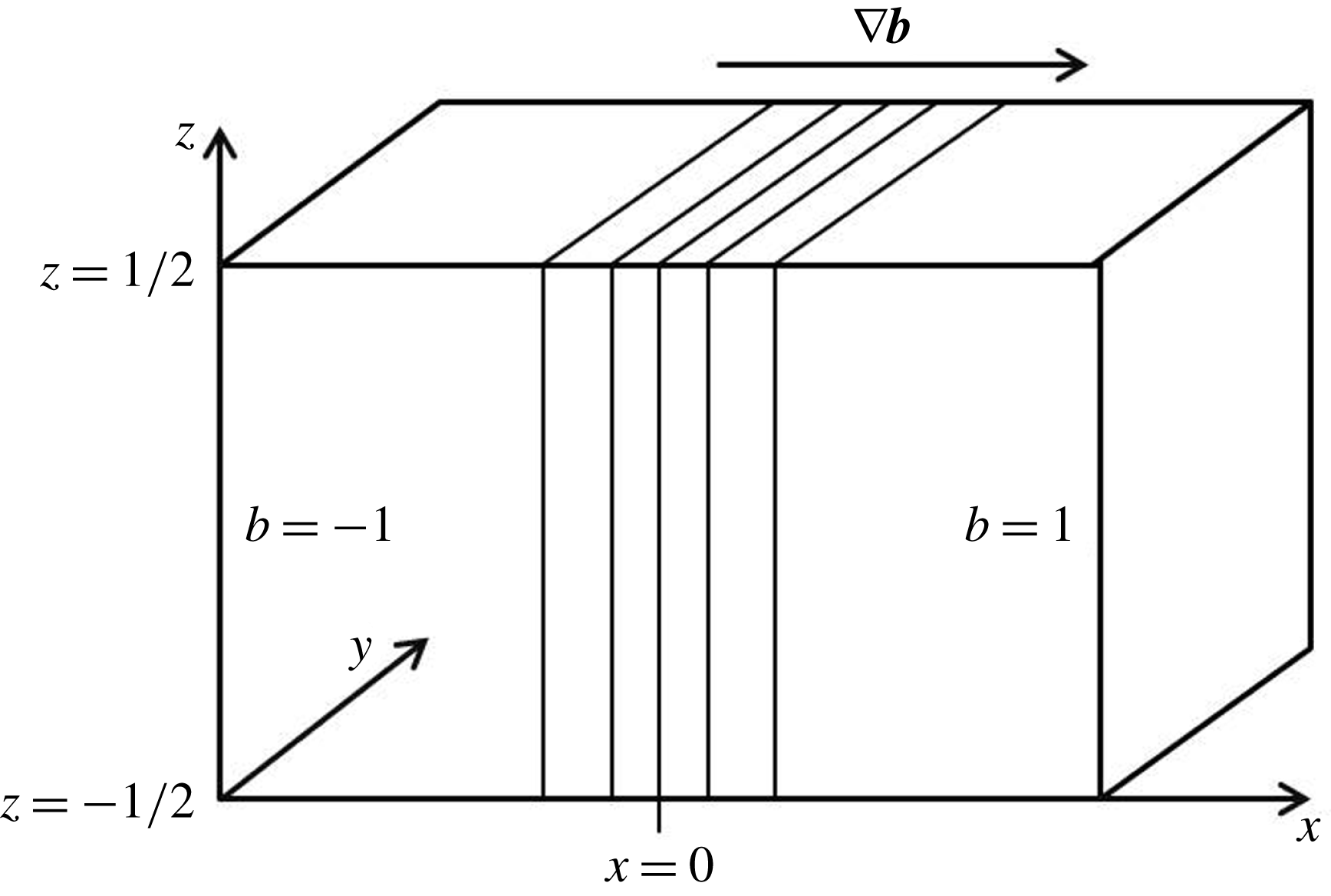
, although we will retain all three components of the velocity vector. We then assume without loss of generality that the front separates low buoyancy fluid on the left from high buoyancy fluid on the right (see figure 1).
Two-dimensional problem set-up. We consider an unbounded
 $x$
domain between two horizontal boundaries at
 $z=\pm 1/2$
with no variations in the along-front,
 $y$
, direction. We non-dimensionalise the horizontal length by
 $L$
, the depth by
 $H$
, horizontal velocity by
 $U$
, vertical velocity by
 $UH/L$
, pressure by
 $fUL$
, buoyancy by
 $fUL/H$
and time by
 $L/U$
. The velocity scale
 $U$
is given by
 $U=\unicode[STIX]{x0394}bH/(fL)$
. Numerically we consider
 $x\in [-L_{x}/2,L_{x}/2]$
and use periodic boundary conditions at the edges on the horizontal domain.

Here, we consider the response of an initially balanced front to an imposed viscosity
 $\unicode[STIX]{x1D708}$
and diffusivity
 $\unicode[STIX]{x1D705}$
which we assume for simplicity are constant. Note that, while
 $\unicode[STIX]{x1D708}$
and
 $\unicode[STIX]{x1D705}$
are assumed to be constant in time, our primary motivation is to study the influence of small-scale turbulence on the evolution of the front. By using a time-independent
 $\unicode[STIX]{x1D708}$
and
 $\unicode[STIX]{x1D705}$
, we are able to isolate the influence of viscosity and diffusion on the evolution of the front without allowing the feedback associated with the front altering the properties of small-scale turbulence. This assumption is very artificial but greatly simplifies the analysis. The set-up can also be viewed as a laboratory-scale analogue with molecular
 $\unicode[STIX]{x1D708}$
and
 $\unicode[STIX]{x1D705}$
. Note that the assumption of constant
 $\unicode[STIX]{x1D708}$
and
 $\unicode[STIX]{x1D705}$
has been used before to study the response of ocean fronts to small-scale turbulence (e.g. Thompson (Reference Thompson2000)).
We can non-dimensionalise the governing equations using a horizontal length scale
 $L$
, vertical length scale
 $H$
and buoyancy scale
 $B$
, with the horizontal velocity scale
 $U=\unicode[STIX]{x0394}bH/(fL)$
, vertical velocity scale
 $W=UH/L=\unicode[STIX]{x0394}bH^{2}/(fL^{2})$
, pressure scale
 $P=fUL=\unicode[STIX]{x0394}bH$
and time scale
 $L/U=fL^{2}/(H\unicode[STIX]{x0394}b)$
for Coriolis parameter
 $f$
. This gives the following non-dimensional equations (Charney Reference Charney1973):
 $$\begin{eqnarray}\displaystyle & \displaystyle Ro\frac{\text{D}u}{\text{D}t}-v=-\frac{\unicode[STIX]{x2202}p}{\unicode[STIX]{x2202}x}+E\,\unicode[STIX]{x1D6FB}_{\unicode[STIX]{x1D716}}^{2}u, & \displaystyle\end{eqnarray}$$
 $$\begin{eqnarray}\displaystyle & \displaystyle Ro\frac{\text{D}v}{\text{D}t}+u=E\,\unicode[STIX]{x1D6FB}_{\unicode[STIX]{x1D716}}^{2}v, & \displaystyle\end{eqnarray}$$
 $$\begin{eqnarray}\displaystyle & \displaystyle Ro\,\unicode[STIX]{x1D716}^{2}\frac{\text{D}w}{\text{D}t}=-\frac{\unicode[STIX]{x2202}p}{\unicode[STIX]{x2202}z}+b+\unicode[STIX]{x1D716}^{2}E\,\unicode[STIX]{x1D6FB}_{\unicode[STIX]{x1D716}}^{2}w, & \displaystyle\end{eqnarray}$$
 $$\begin{eqnarray}\displaystyle & \displaystyle Ro\frac{\text{D}b}{\text{D}t}=\frac{E}{Pr}\,\unicode[STIX]{x1D6FB}_{\unicode[STIX]{x1D716}}^{2}b, & \displaystyle\end{eqnarray}$$
 $$\begin{eqnarray}\displaystyle & \displaystyle \frac{\unicode[STIX]{x2202}u}{\unicode[STIX]{x2202}x}+\frac{\unicode[STIX]{x2202}v}{\unicode[STIX]{x2202}y}+\frac{\unicode[STIX]{x2202}w}{\unicode[STIX]{x2202}z}=0, & \displaystyle\end{eqnarray}$$
 $\text{D}/\text{D}t$
and
 $\unicode[STIX]{x1D6FB}_{\unicode[STIX]{x1D716}}$
are given by
 $$\begin{eqnarray}\displaystyle & \displaystyle \frac{\text{D}}{\text{D}t}=\frac{\unicode[STIX]{x2202}}{\unicode[STIX]{x2202}t}+u\frac{\unicode[STIX]{x2202}}{\unicode[STIX]{x2202}x}+w\frac{\unicode[STIX]{x2202}}{\unicode[STIX]{x2202}z}, & \displaystyle\end{eqnarray}$$
 $$\begin{eqnarray}\displaystyle & \displaystyle \unicode[STIX]{x1D6FB}_{\unicode[STIX]{x1D716}}^{2}=\frac{\unicode[STIX]{x2202}^{2}}{\unicode[STIX]{x2202}z^{2}}+\unicode[STIX]{x1D716}^{2}\frac{\unicode[STIX]{x2202}^{2}}{\unicode[STIX]{x2202}x^{2}}, & \displaystyle\end{eqnarray}$$
 $\unicode[STIX]{x1D716}=H/L$
.
Definitions of the dimensionless parameters and their values for buoyancy difference,
 $\unicode[STIX]{x0394}b$
, Coriolis parameter,
 $f$
, horizontal length scale,
 $L$
, vertical length scale,
 $H$
, and viscosity and diffusivity,
 $\unicode[STIX]{x1D708}$
and
 $\unicode[STIX]{x1D705}$
.

We will take
 $Pr=1$
, use boundary conditions of no vertical shear, vertical velocity or buoyancy flux on the top and bottom boundaries and consider a fluid layer between
 $z=\pm 0.5$
for unbounded
 $x$
. This set-up is a slightly simplified version of the set-up used in Crowe & Taylor (Reference Crowe and Taylor2018) which consisted of a three-dimensional model with arbitrary
 $Pr$
.
3 Numerical simulations
We use numerical simulations to study the time evolution of an initially depth independent front,
 $b|_{t=0}=b(x)$
. The numerical simulations are carried out using DIABLO. Time stepping is performed with a combination of explicit third-order Runge–Kutta and implicit Crank–Nicolson schemes while finite differences are used for derivatives in the vertical direction and discrete Fourier transforms, using the pseudo-spectral method for nonlinear terms, are used for derivatives in the horizontal direction (Taylor Reference Taylor2008).
In order to use periodic boundary conditions in the horizontal direction we subtract a linear profile from the buoyancy and define
 $$\begin{eqnarray}b^{\prime }=b-\frac{2x}{L_{x}},\end{eqnarray}$$
and
 $$\begin{eqnarray}p^{\prime }=p-\frac{2xz}{L_{x}},\end{eqnarray}$$
where
 $L_{x}$
is the horizontal domain width so at
 $x=\pm L_{x}/2$
we have
 $b^{\prime }=0$
. Equation (2.1) becomes
 $$\begin{eqnarray}\displaystyle & \displaystyle Ro\frac{\text{D}u}{\text{D}t}-v=-\frac{\unicode[STIX]{x2202}p^{\prime }}{\unicode[STIX]{x2202}x}-\frac{2z}{L_{x}}+E\,\unicode[STIX]{x1D6FB}_{\unicode[STIX]{x1D716}}^{2}u, & \displaystyle\end{eqnarray}$$
 $$\begin{eqnarray}\displaystyle & \displaystyle Ro\frac{\text{D}v}{\text{D}t}+u=E\,\unicode[STIX]{x1D6FB}_{\unicode[STIX]{x1D716}}^{2}v, & \displaystyle\end{eqnarray}$$
 $$\begin{eqnarray}\displaystyle & \displaystyle Ro\,\unicode[STIX]{x1D716}^{2}\frac{\text{D}w}{\text{D}t}=-\frac{\unicode[STIX]{x2202}p^{\prime }}{\unicode[STIX]{x2202}z}+b^{\prime }+\unicode[STIX]{x1D716}^{2}E\,\unicode[STIX]{x1D6FB}_{\unicode[STIX]{x1D716}}^{2}w, & \displaystyle\end{eqnarray}$$
 $$\begin{eqnarray}\displaystyle & \displaystyle Ro\frac{\text{D}b^{\prime }}{\text{D}t}+\frac{2Ro\,u}{L_{x}}=\frac{E}{Pr}\,\unicode[STIX]{x1D6FB}_{\unicode[STIX]{x1D716}}^{2}b^{\prime }, & \displaystyle\end{eqnarray}$$
 $$\begin{eqnarray}\displaystyle & \displaystyle \frac{\unicode[STIX]{x2202}u}{\unicode[STIX]{x2202}x}+\frac{\unicode[STIX]{x2202}v}{\unicode[STIX]{x2202}y}+\frac{\unicode[STIX]{x2202}w}{\unicode[STIX]{x2202}z}=0, & \displaystyle\end{eqnarray}$$
 $(u,v,w,b^{\prime },p^{\prime })$
with horizontally periodic boundary conditions.
Due to the large Ekman numbers used, the maximum time step is set by the condition that the diffusive length scale per time step is less than the horizontal grid scale. Therefore, the time step,
 $\unicode[STIX]{x0394}t$
is chosen to be
 $$\begin{eqnarray}\unicode[STIX]{x0394}t=C\frac{Ro}{E},\end{eqnarray}$$
where
 $C$
is a constant determined by the grid scale,
 $\unicode[STIX]{x0394}x=L_{x}/N_{x}$
. From Crowe & Taylor (Reference Crowe and Taylor2018) we expect the depth-averaged buoyancy field to evolve on the slow time scale
 $$\begin{eqnarray}T=Ro\,t,\end{eqnarray}$$
so we run each simulation until
 $t_{end}=10^{3}/Ro$
. The required number of time steps is therefore
 $$\begin{eqnarray}N_{t}=\frac{10^{3}E}{C\,Ro^{2}}.\end{eqnarray}$$
We use a grid resolution of
 $N_{x}=256$
and a domain width of
 $L_{x}=10$
which requires a value of
 $C=10^{-3}$
for accuracy.
Finally, we impose the initial condition
 $$\begin{eqnarray}b(x)=\tanh x,\end{eqnarray}$$
and set the initial velocity using the leading-order TTW solution (Gula, Molemaker & McWilliams Reference Gula, Molemaker and McWilliams2014; McWilliams Reference McWilliams2017; Crowe & Taylor Reference Crowe and Taylor2018),
 $$\begin{eqnarray}\displaystyle & \displaystyle u=-\sqrt{E}\,K_{0}^{\prime \prime }(z/\sqrt{E};\unicode[STIX]{x1D701}_{0})\frac{\unicode[STIX]{x2202}b}{\unicode[STIX]{x2202}x}, & \displaystyle\end{eqnarray}$$
 $$\begin{eqnarray}\displaystyle & \displaystyle v=-\sqrt{E}\,K_{0}(z/\sqrt{E};\unicode[STIX]{x1D701}_{0})\frac{\unicode[STIX]{x2202}b}{\unicode[STIX]{x2202}x}, & \displaystyle\end{eqnarray}$$
 $$\begin{eqnarray}\displaystyle & \displaystyle w=E\,K_{0}^{\prime }(z/\sqrt{E};\unicode[STIX]{x1D701}_{0})\frac{\unicode[STIX]{x2202}^{2}b}{\unicode[STIX]{x2202}x^{2}}, & \displaystyle\end{eqnarray}$$
 $$\begin{eqnarray}K_{0}(\unicode[STIX]{x1D701};\unicode[STIX]{x1D701}_{0})=-\unicode[STIX]{x1D701}+C_{+}(\unicode[STIX]{x1D701}_{0})\operatorname{cs}(\unicode[STIX]{x1D701})+C_{-}(\unicode[STIX]{x1D701}_{0})\operatorname{sc}(\unicode[STIX]{x1D701}),\end{eqnarray}$$
for the functions
 $$\begin{eqnarray}\left.\begin{array}{@{}c@{}}\operatorname{cc}(\unicode[STIX]{x1D701})=\cosh (\unicode[STIX]{x1D701}/\sqrt{2})\cos (\unicode[STIX]{x1D701}/\sqrt{2}),\\ \operatorname{cs}(\unicode[STIX]{x1D701})=\cosh (\unicode[STIX]{x1D701}/\sqrt{2})\sin (\unicode[STIX]{x1D701}/\sqrt{2}),\\ \operatorname{ss}(\unicode[STIX]{x1D701})=\sinh (\unicode[STIX]{x1D701}/\sqrt{2})\sin (\unicode[STIX]{x1D701}/\sqrt{2}),\\ \operatorname{sc}(\unicode[STIX]{x1D701})=\sinh (\unicode[STIX]{x1D701}/\sqrt{2})\cos (\unicode[STIX]{x1D701}/\sqrt{2}),\end{array}\right\}\end{eqnarray}$$
and constants
 $$\begin{eqnarray}C_{\pm }(\unicode[STIX]{x1D701}_{0})=\frac{1}{\sqrt{2}}\frac{\operatorname{cc}(\unicode[STIX]{x1D701}_{0})\pm \operatorname{ss}(\unicode[STIX]{x1D701}_{0})}{\operatorname{cc}^{2}(\unicode[STIX]{x1D701}_{0})+\operatorname{ss}^{2}(\unicode[STIX]{x1D701}_{0})},\end{eqnarray}$$
and
 $\unicode[STIX]{x1D701}_{0}=1/\sqrt{4E}$
. See appendix A of Crowe & Taylor (Reference Crowe and Taylor2018) for details. Note that the velocity reduces to the linear ‘thermal wind’ velocity profile,
 $K_{0}(\unicode[STIX]{x1D701})\sim -\unicode[STIX]{x1D701}$
, in the limit of small Ekman number. We expect some initial adjustment as the front slumps and
 $b$
develops a small, order-
 $Ro$
, depth dependence. However, we do not expect significant inertial oscillations since the velocity field is in TTW balance at
 $t-0$
. We perform simulations for 20 different Ekman numbers between
 $E=0.01$
and
 $E=1$
and 9 different Rossby numbers between
 $Ro=0.1$
and
 $Ro=1$
for a total of 180 simulations.
4 Results
We now compare the results of our numerical simulations with our theoretical predictions. We begin by examining the spreading rate of the front and the accuracy of the theory for
 $O(1)$
Rossby numbers. We will then examine frontogenesis during the transient adjustment. Finally, we will derive and test a scaling for the maximum vertical velocity.
4.1 Spreading rate
In Crowe & Taylor (Reference Crowe and Taylor2018) we found that over long times the leading order buoyancy profile,
 $b_{0}$
, becomes self-similar with a form given by
 $$\begin{eqnarray}b_{0}=F\left(\frac{x}{\unicode[STIX]{x1D6FE}(T+T_{0})^{1/4}}\right),\end{eqnarray}$$
where
 $$\begin{eqnarray}F(\unicode[STIX]{x1D702})=\left\{\begin{array}{@{}ll@{}}-1,\quad & \unicode[STIX]{x1D702}<-4/\unicode[STIX]{x03C0},\\ \displaystyle \frac{1}{2}\left[\unicode[STIX]{x1D702}\sqrt{1-\frac{\unicode[STIX]{x03C0}^{2}\unicode[STIX]{x1D702}^{2}}{16}}+\frac{4}{\unicode[STIX]{x03C0}}\arcsin \left(\frac{\unicode[STIX]{x03C0}\unicode[STIX]{x1D702}}{4}\right)\right],\quad & \unicode[STIX]{x1D702}\in \left[-4/\unicode[STIX]{x03C0},4/\unicode[STIX]{x03C0}\right]\\ 1,\quad & \unicode[STIX]{x1D702}>4/\unicode[STIX]{x03C0},\end{array}\right.,\end{eqnarray}$$
where
 $\unicode[STIX]{x1D6FE}$
is the spreading parameter and
 $T_{0}$
describes the time taken for the solution to reach a self-similar state. The spreading parameter can be linked to the frontal width by
 $$\begin{eqnarray}l_{f}(T)=\frac{8\unicode[STIX]{x1D6FE}(T+T_{0})^{1/4}}{\unicode[STIX]{x03C0}}.\end{eqnarray}$$
We now compare the numerically observed spreading with this theoretical prediction. In some simulations fast spreading results in the front reaching the edges of the horizontal domain so we choose a time interval of
 $T\in [100,350]$
for the analysis, during which time the transients have decayed and, for most simulations, the front has not reached the edges of the domain. For this time interval we assume that the front is self-similar with a centreline (
 $z=0$
) buoyancy of the form
 $$\begin{eqnarray}b=F\left(\frac{x}{f(T)}\right).\end{eqnarray}$$
We now fit this prediction to the numerical centreline buoyancy field to determine
 $f(T)$
and finally fit
 $f(T)$
to the curve
 $$\begin{eqnarray}f(T)=\unicode[STIX]{x1D6FE}_{n}(T+T_{0n})^{\unicode[STIX]{x1D6FC}_{n}},\end{eqnarray}$$
to determine the values of
 $(\unicode[STIX]{x1D6FE}_{n},T_{0n},\unicode[STIX]{x1D6FC}_{n})$
for each pair of parameters,
 $(Ro,E)$
. All fitting is done using a least squares method. From Crowe & Taylor (Reference Crowe and Taylor2018) we expect that the predicted spreading rate is valid for
 $$\begin{eqnarray}T\ll T_{max}=\frac{Ro^{4}Pr^{3}Q(E)}{\unicode[STIX]{x1D716}^{4}E^{2}},\end{eqnarray}$$
where
 $$\begin{eqnarray}Q(E)=E\int _{-1/2}^{1/2}(K_{0}^{\prime })^{2}\,\text{d}z\end{eqnarray}$$
and
 $$\begin{eqnarray}Pr\,Q(E)=\frac{4\unicode[STIX]{x1D6FE}^{4}}{3\unicode[STIX]{x03C0}^{2}}\end{eqnarray}$$
is proportional to the effective horizontal diffusivity resulting from shear dispersion. This condition comes from the requirement that shear dispersion dominates horizontal diffusion. Note that horizontal diffusion becomes important sooner when
 $Ro$
is small or
 $E$
is large. When both
 $E$
is large and
 $Ro$
is small, the horizontal diffusion is fast and the front quickly spreads to fill the domain, therefore we do not expect the predicted spreading rate to be accurate in this region.
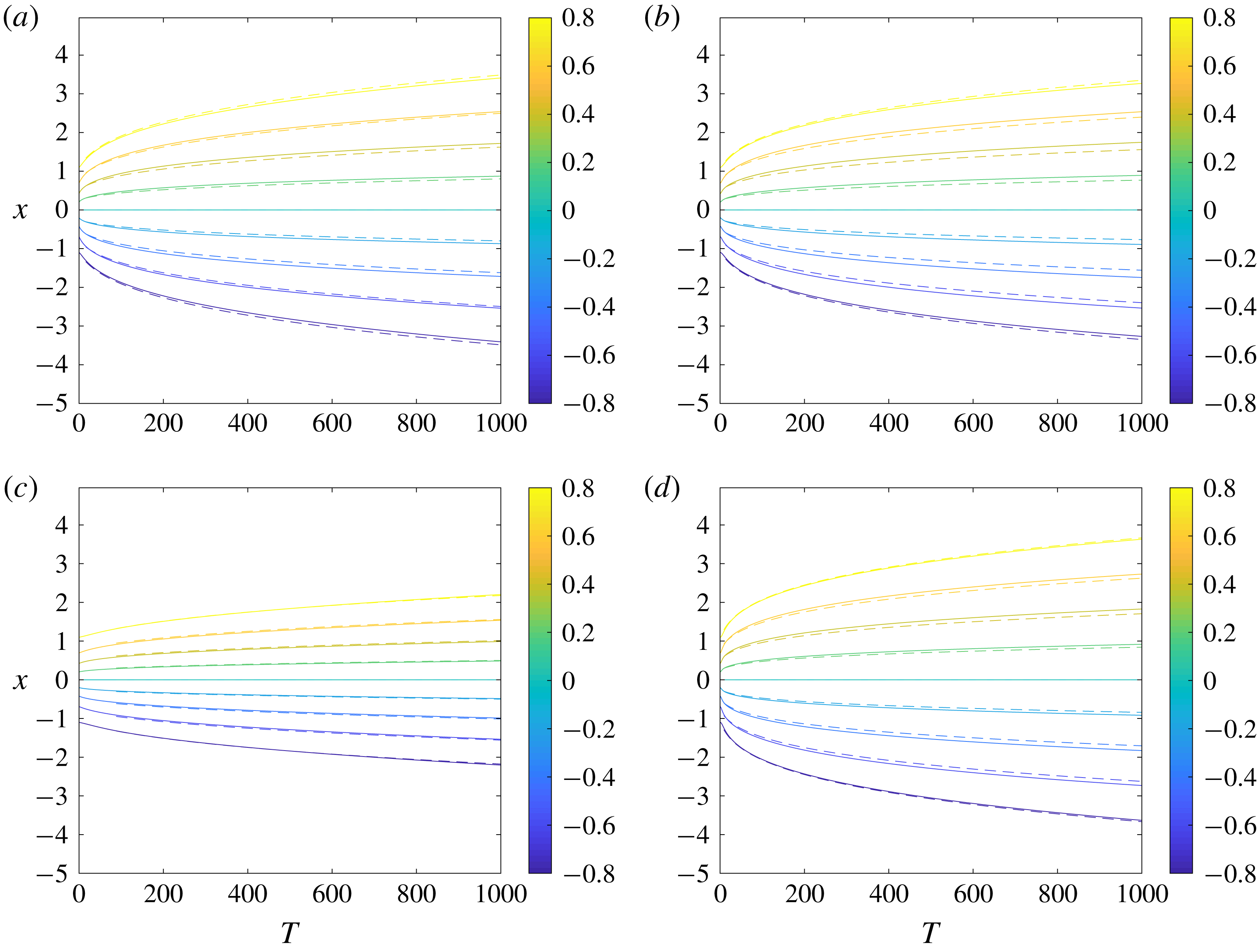
Plots of
 $b(x,z,T)$
at
 $z=0$
for (a)
 $Ro=0.1,E=0.02$
, (b)
 $Ro=0.5,E=0.02$
, (c)
 $Ro=0.5,E=0.3$
and (d)
 $Ro=1,E=0.06$
. The solid contours show our simulation results while the dashed contours show the theoretical predictions using the numerical values of
 $(\unicode[STIX]{x1D6FE}_{n},T_{0n},\unicode[STIX]{x1D6FC}_{n})$
.

Figure 2 shows the centreline (
 $z=0$
) buoyancy fields as functions of
 $x$
and
 $T$
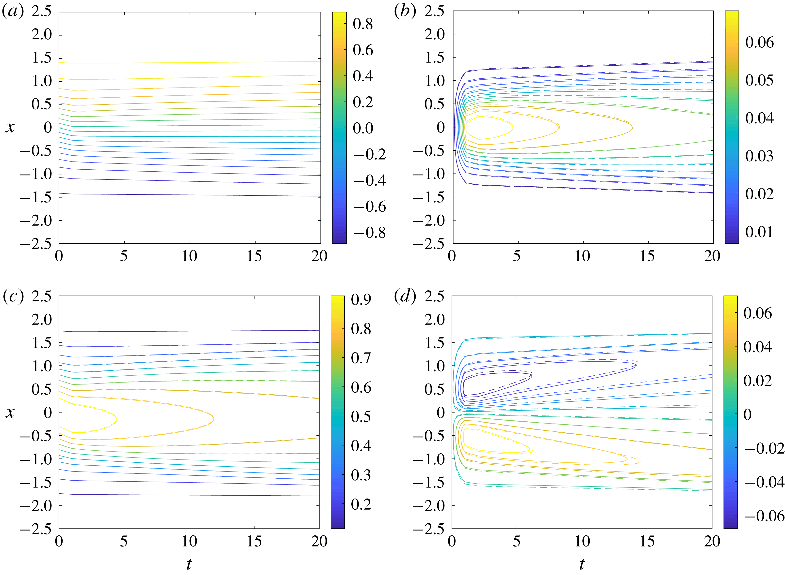
for a variety of Rossby and Ekman numbers. The theoretical predictions are given by the dashed contours. In each case the long term behaviour exhibits frontal spreading. This spreading is well described by the predictions, even for the case of larger Rossby numbers where the theoretical predictions are not asymptotically valid. Figure 2(a,b) shows the centreline buoyancy for
 $E=0.02$
and two different Rossby numbers. The long term spreading is similar in each case when plotted as a function of the slow time scale,
 $T=Rot$
. This is consistent with the theoretical similarity solution which depends on
 $Ro$
only through
 $T$
. Note that the edges of the front appear more diffuse for smaller Rossby numbers; this is expected since horizontal diffusion becomes important at earlier times for smaller Rossby numbers.
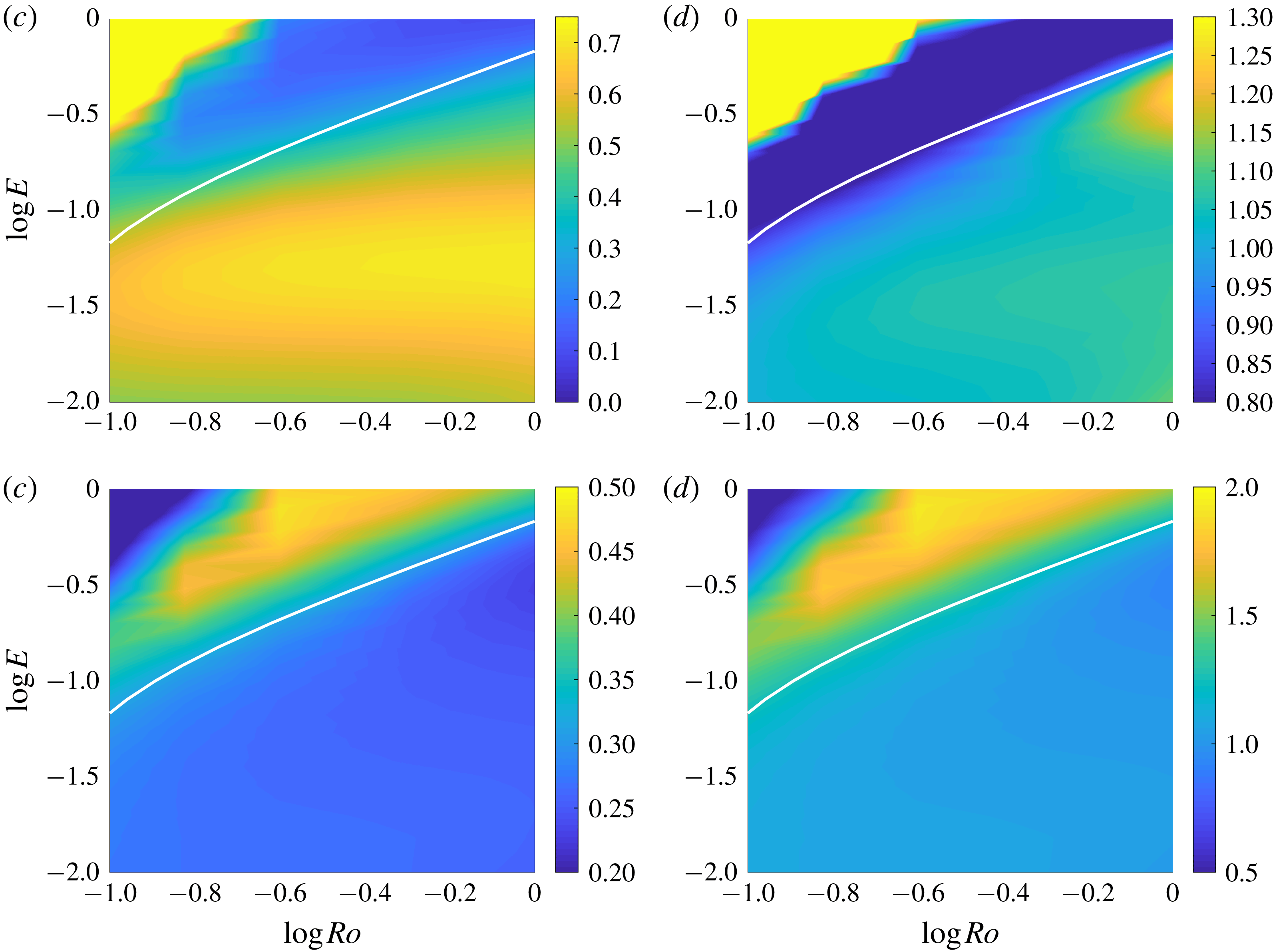
Plots of (a)
 $\unicode[STIX]{x1D6FE}_{n}$
, (b)
 $\unicode[STIX]{x1D6FE}_{n}/\unicode[STIX]{x1D6FE}$
, (c)
 $\unicode[STIX]{x1D6FC}_{n}$
, (d)
 $\unicode[STIX]{x1D6FC}_{n}/\unicode[STIX]{x1D6FC}$
as functions of
 $E$
and
 $Ro$
. We use a time interval of
 $[100,350]$
and also plot the curve
 $T_{max}=3500$
in white.

Figure 3 shows the values of
 $\unicode[STIX]{x1D6FE}_{n}$
and
 $\unicode[STIX]{x1D6FC}_{n}$
calculated over the time interval
 $[100,350]$
and the ratio of these numerical values with the theoretical predictions for
 $\unicode[STIX]{x1D6FE}$
and
 $\unicode[STIX]{x1D6FC}$
. We expect our theory to be valid for
 $T<T_{max}/10$
and plot the curve
 $T_{max}=3500$
in white. The region below this curve is where the theory should be valid. The values of
 $\unicode[STIX]{x1D6FE}_{n}$
and
 $\unicode[STIX]{x1D6FC}_{n}$
match the theoretical predictions within 10 %–20 %. In the region where we expect horizontal diffusion to dominate,
 $\unicode[STIX]{x1D6FC}_{n}\approx 1/2$
, which is consistent with diffusive spreading. The front has filled the computational domain in the cases with large
 $E$
and small
 $Ro$
so the results in the top left regions of each figure are not reflective of the true spreading rate.
From figure 3(a) we can see that the spreading rate,
 $\unicode[STIX]{x1D6FE}_{n}$
, is approximately independent of
 $Ro$
below the curve
 $T_{max}=3500$
. This matches our theoretical prediction where
 $\unicode[STIX]{x1D6FE}$
depends only on
 $E$
and
 $Pr$
though interestingly the prediction is still valid for
 $Ro=O(1)$
. Similarly the prediction of
 $\unicode[STIX]{x1D6FC}=1/4$
is accurate for the case of
 $Ro=O(1)$
which suggests that spreading via shear dispersion is still the dominant mechanism and the theory is valid for order-
 $1$
Rossby numbers despite being derived in the small
 $Ro$
limit. We now consider the
 $Ro=O(1)$
simulations in more detail to see how accurately the theory predicts the form of the velocity and buoyancy fields.
4.2 Accuracy of theory for O(1) Rossby numbers
Since the theoretical predictions in Crowe & Taylor (Reference Crowe and Taylor2018) were made in the limit of small
 $Ro$
, these predictions do not necessarily hold in the case of
 $Ro=O(1)$
where the nonlinear advection terms in the momentum and buoyancy equations are no longer small. Despite this, we have seen above that the spreading rate of the front when
 $Ro=1$
is still accurately captured by the theoretical predictions. We now examine the velocity and buoyancy fields for the
 $Ro=1$
case in more detail to determine how accurately they are described by the linear TTW solution in Crowe & Taylor (Reference Crowe and Taylor2018).
The two-dimensional streamfunction,
 $\unicode[STIX]{x1D713}(x,z,t)$
, describing the circulation around the front is defined by
 $u=\unicode[STIX]{x2202}\unicode[STIX]{x1D713}/\unicode[STIX]{x2202}z$
and
 $w=-\unicode[STIX]{x2202}\unicode[STIX]{x1D713}/\unicode[STIX]{x2202}x$
. We define
 $$\begin{eqnarray}\unicode[STIX]{x1D713}_{n}=\int _{-0.5}^{z}u(x,z^{\prime },t)\,\text{d}z^{\prime },\end{eqnarray}$$
and calculate
 $\unicode[STIX]{x1D713}_{n}$
by numerically integrating the velocity fields from the simulations. We compare
 $\unicode[STIX]{x1D713}_{n}$
to the leading-order analytic prediction
 $$\begin{eqnarray}\unicode[STIX]{x1D713}_{0}=-E\,K_{0}^{\prime }(z/\sqrt{E})\frac{\unicode[STIX]{x2202}b}{\unicode[STIX]{x2202}x},\end{eqnarray}$$
and define the difference between the analytic and numerical values of the streamfunction by
 $$\begin{eqnarray}\unicode[STIX]{x0394}\unicode[STIX]{x1D713}=\unicode[STIX]{x1D713}_{n}-\unicode[STIX]{x1D713}_{0}.\end{eqnarray}$$
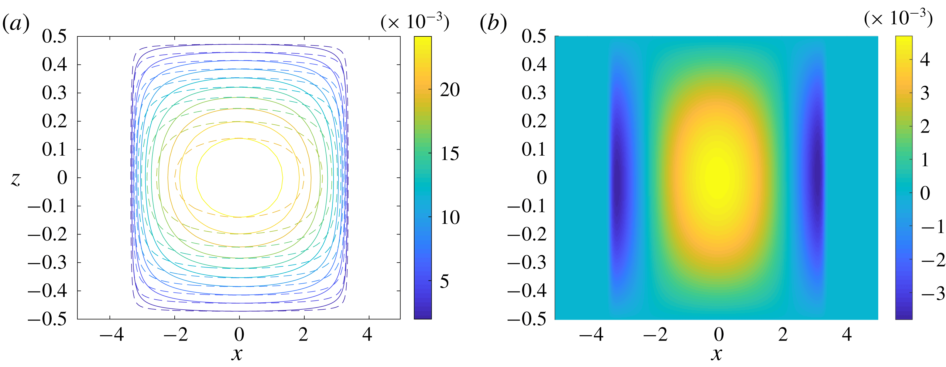
Plots of (a)
 $\unicode[STIX]{x1D713}_{n}$
(solid) and
 $\unicode[STIX]{x1D713}_{0}$
(dashed) (b)
 $\unicode[STIX]{x0394}\unicode[STIX]{x1D713}$
. Results are given for
 $Ro=1$
,
 $E=0.1$
and
 $T=300$
.

Figure 4 shows
 $\unicode[STIX]{x1D713}_{n}$
,
 $\unicode[STIX]{x1D713}_{0}$
and
 $\unicode[STIX]{x0394}\unicode[STIX]{x1D713}$
for
 $Ro=1$
and
 $E=0.1$
at
 $T=300$
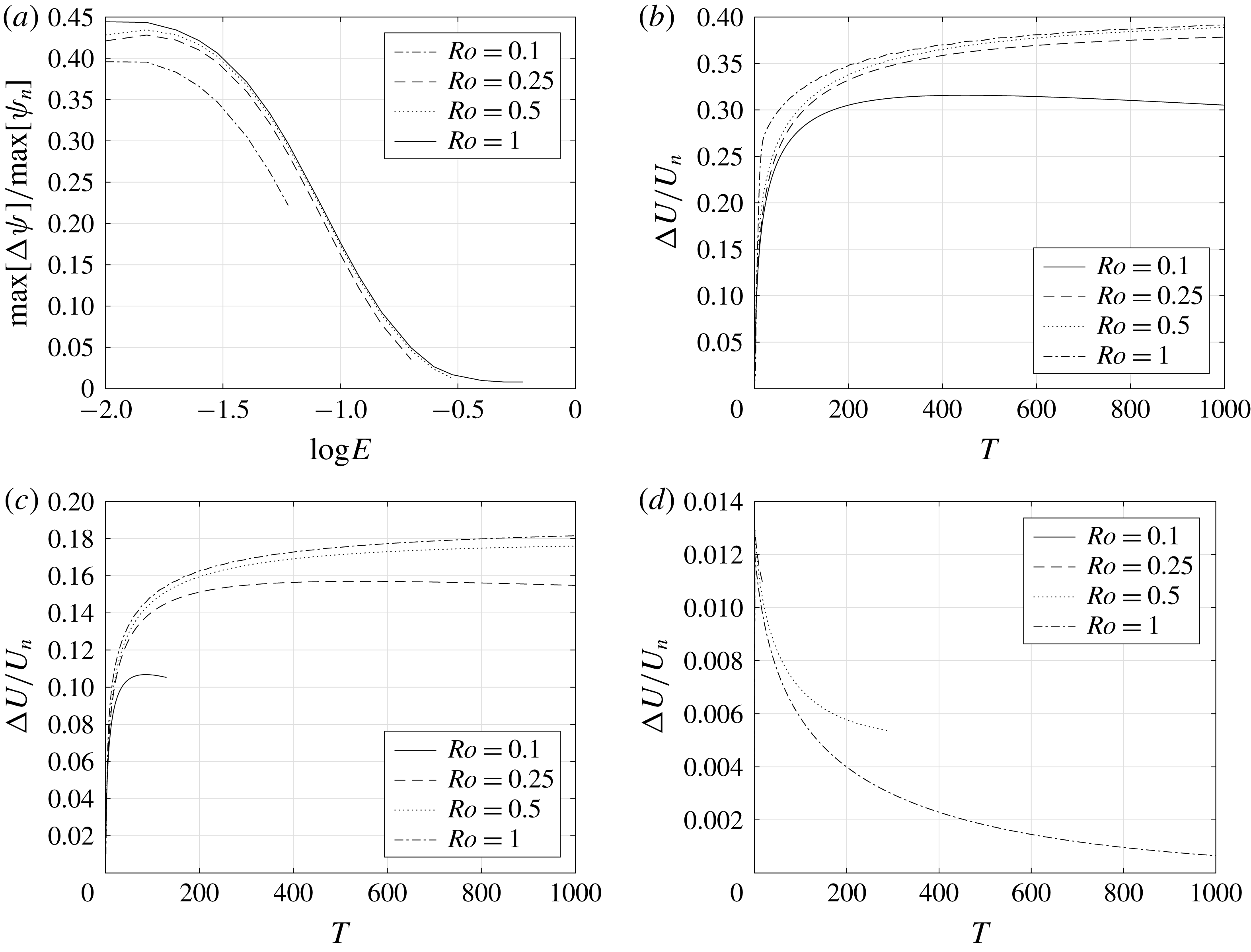
. We can see that the leading order analytic prediction is fairly accurate, with a maximum magnitude within 20 % of the numerical value. The main difference is the shape of the contours with the contours of
 $\unicode[STIX]{x1D713}_{n}$
being more circular than those of
 $\unicode[STIX]{x1D713}_{0}$
.
Figure 5(a) shows the normalised maximum difference between
 $\unicode[STIX]{x1D713}_{0}$
and
 $\unicode[STIX]{x1D713}_{n}$
,
 $\max [\unicode[STIX]{x0394}\unicode[STIX]{x1D713}]/\text{max}[\unicode[STIX]{x1D713}_{n}]$
. Interestingly, we can see that the deviation of
 $\unicode[STIX]{x1D713}$
is more strongly dependent on Ekman number than on Rossby number and the predictions for
 $Ro=1$
are not significantly less accurate than for smaller Rossby numbers while the predictions for large
 $E$
are much more accurate than for small
 $E$
. It is notable that the theoretical prediction performs nearly as well for
 $Ro=1$
compared to smaller Rossby numbers, despite the fact that the theory was derived using an asymptotic expansion valid for
 $Ro\ll 1$
. The relatively poor performance of the theory for small
 $E$
will be examined later.
(a) Value of
 $\max [\unicode[STIX]{x0394}\unicode[STIX]{x1D713}]/\max [\unicode[STIX]{x1D713}_{n}]$
as a function of
 $E$
for
 $T=300$
. Results are shown where
 $T_{max}<3000$
for a range of
 $Ro$
. (b–d) Value of
 $\unicode[STIX]{x0394}U/U_{n}$
as a function of
 $T$
for (b)
 $E=0.02$
, (c)
 $E=0.1$
and (d)
 $E=0.4$
and a range of
 $Ro$
. Results are shown up to
 $T=T_{max}/10$
.

The maximum cross-front velocity,
 $U(t)$
, is given by
 $$\begin{eqnarray}U(t)=\left|\max _{x,z}[u]\right|,\end{eqnarray}$$
and using the leading-order analytic solution, our prediction for the maximum cross-front velocity is
 $$\begin{eqnarray}U_{0}=u_{0}(0,1/2,t)=\sqrt{E}\,K_{0}^{\prime \prime }(1/2\sqrt{E})\left.\frac{\unicode[STIX]{x2202}b}{\unicode[STIX]{x2202}x}\right|_{x,z=0}.\end{eqnarray}$$
From the numerical simulations we define
 $U_{n}(t)$
to be the maximum value of
 $u$
at each time and
 $\unicode[STIX]{x0394}U=|U_{n}-U_{0}|$
to be the difference between the numerical data and the theoretical prediction. Figure 5(b–d) shows the error in the prediction of the maximum cross-front velocity, given by
 $\unicode[STIX]{x0394}U/U_{n}$
, for
 $E=0.02$
,
 $E=0.1$
and
 $E=0.4$
. We can see that the error is largest for small
 $E$
and is not strongly affected by increasing the Rossby number from
 $Ro=0.1$
to
 $Ro=1$
. We might anticipate that over long times the error will decrease as the neglected higher-order terms of
 $u$
should decay faster than the leading-order term
 $u_{0}$
since they depend on higher powers and derivatives of
 $\unicode[STIX]{x2202}b_{0}/\unicode[STIX]{x2202}x$
and hence they depend on higher powers of
 $1/(T+T_{0})^{\unicode[STIX]{x1D6FC}}$
. This interpretation is supported by the numerical data as shown in figure 5(b–d) where the error appears to gradually decrease over long times after an initial increase. Note that the duration of the initial increase may exceed the time window for some parameter ranges. This is most apparent for the cases of lowest
 $Ro$
and highest
 $E$
suggesting that this time scale scales as
 $Ro^{a}/E^{b}$
for positive
 $a$
and
 $b$
. We examine the case of small
 $E$
in detail in § 5.
Comparison of the centreline buoyancy at
 $T=250$
as a function of
 $\unicode[STIX]{x1D702}=x/\unicode[STIX]{x1D6FE}(T+T_{0})^{1/4}$
with the similarity solution,
 $F(\unicode[STIX]{x1D702})$
for (a)
 $Ro=0.5$
,
 $E=0.04$
, (b)
 $Ro=0.5$
,
 $E=0.1$
, (c)
 $Ro=1$
,
 $E=0.04$
and (d)
 $Ro=1$
,
 $E=0.1$
.

From Crowe & Taylor (Reference Crowe and Taylor2018) the theoretical prediction of the centreline, (
 $z=0$
), buoyancy is
 $$\begin{eqnarray}b|_{z=0}=b_{0}+O(Ro^{2}),\end{eqnarray}$$
where
 $b_{0}$
is given by (4.1). Note that the order
 $Ro$
contribution has odd vertical symmetry and hence is zero along the centreline. We now compare this prediction with the numerical results by examining the shape of the cross-front buoyancy profiles from the numerical simulations.
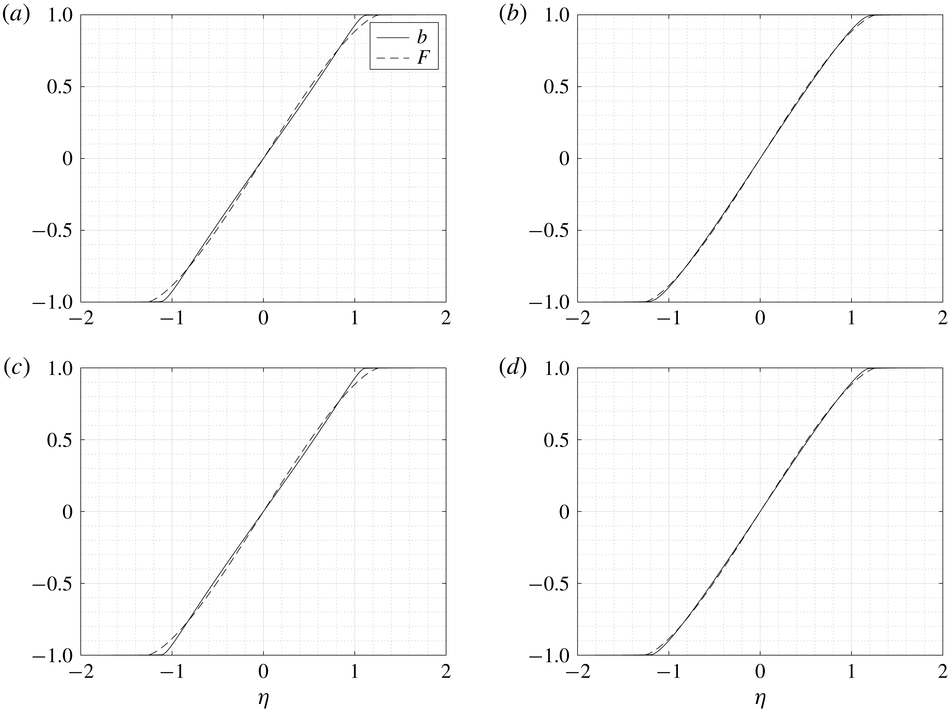
Figure 6 shows the centreline buoyancy profiles as a function of the normalised cross-front distance at
 $T=250$
for a range of Rossby and Ekman numbers. We can see that the profiles are approximately linear in the centre of the horizontal domain and more closely match the similarity solution for larger Ekman numbers. The size of the Rossby number has very little effect on the profile, even when
 $Ro=O(1)$
, though when diffusive effects are large, corresponding to large
 $E$
and small
 $Ro$
, the effects of this diffusion can be seen near the edges of the front which are less sharp and wider.
4.3 Initial frontogenesis
In Crowe & Taylor (Reference Crowe and Taylor2018) we did not observe strong frontogenesis resulting from the evolution of an initially depth-independent front towards a balanced state. We found time-dependent solutions for this evolution, and saw that it was possible for surface gradients to sharpen during the initial adjustment even though the front was spreading in a depth-averaged sense, however this sharpening is an order
 $Ro$
effect. We now consider the numerical simulations where
 $Ro=O(1)$
to determine if these cases exhibit significant frontogenesis.
In Crowe & Taylor (Reference Crowe and Taylor2018) we found that the order-
 $Ro$
buoyancy component,
 $b_{1}$
, is given by
 $$\begin{eqnarray}b_{1}=-\sqrt{E}\left[K_{0}+\mathop{\sum }_{n=0}^{\infty }D_{n}{\mathcal{Z}}_{n}(z)e^{-E\unicode[STIX]{x1D706}_{n}t/Ro}\right]\left|\unicode[STIX]{x1D6FB}_{H}b_{0}\right|^{2},\end{eqnarray}$$
using the initial condition
 $b_{1}=0$
. The
 $D_{n}$
are given by
 $$\begin{eqnarray}D_{n}=-\frac{1}{z_{n}^{2}}\int _{-1/2}^{1/2}K_{0}{\mathcal{Z}}_{n}\,\text{d}z,\end{eqnarray}$$
where the
 ${\mathcal{Z}}_{n}$
are vertical structure functions, the
 $\unicode[STIX]{x1D706}_{n}$
are their corresponding eigenvalues and the
 $z_{n}$
are normalisation constants, see appendix A of Crowe & Taylor (Reference Crowe and Taylor2018) for details. The cross-front buoyancy gradient can now be calculated as
 $$\begin{eqnarray}M^{2}=\frac{\unicode[STIX]{x2202}b_{0}}{\unicode[STIX]{x2202}x}+Ro\frac{\unicode[STIX]{x2202}b_{1}}{\unicode[STIX]{x2202}x}+O(Ro^{2}),\end{eqnarray}$$
and since we have seen that
 $b_{0}$
only spreads throughout the evolution, any sharpening must appear though the
 $O(Ro)$
term assuming that the
 $O(Ro^{2})$
term is small. This analysis is not asymptotically valid for
 $Ro=O(1)$
so we now seek to determine if significant surface frontogenesis occurs for larger Rossby numbers and how closely the behaviour is described by the analytic predictions.
Plots of the maximum surface horizontal buoyancy gradient,
 $\max _{x}[M^{2}(x,1/2,t)]$
as a function of time,
 $t$
, for a range of Rossby numbers and (a)
 $E=0.01$
and (b)
 $E=0.1$
.

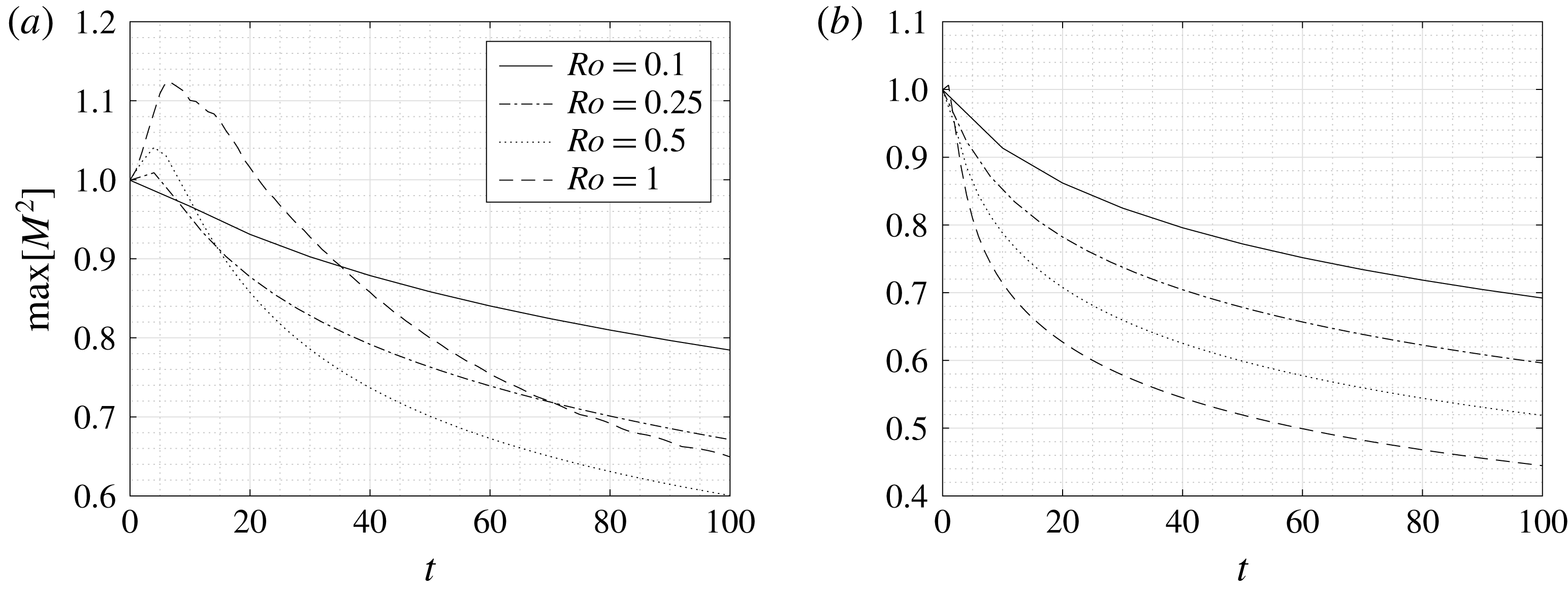
Figure 7 shows the maximum horizontal buoyancy gradient on the top surface for a range of Rossby numbers. We can see that there is some surface sharpening of the front for small Ekman numbers however this effect is relatively small and short lived as once a self-similar state is reached the front will only spread.
Values of (a)
 $b_{0}(x,1/2,t)$
, (b)
 $b_{0}(x,1/2,t)-b_{0}(x,0,t)$
, (c)
 $M^{2}(x,1/2,t)$
and (d)
 $M^{2}(x,1/2,t)-M^{2}(x,0,t)$
for
 $Ro=1$
and
 $E=0.02$
. The solid contours show the numerical results and the dashed contours show the analytic predictions to order
 $O(Ro)$
.

Values of (a)
 $b_{0}(x,1/2,t)$
, (b)
 $b_{0}(x,1/2,t)-b_{0}(x,0,t)$
, (c)
 $M^{2}(x,1/2,t)$
and (d)
 $M^{2}(x,1/2,t)-M^{2}(x,0,t)$
for
 $Ro=1$
and
 $E=0.2$
. The solid contours show the numerical results and the dashed contours show the analytic predictions to order
 $O(Ro)$
.

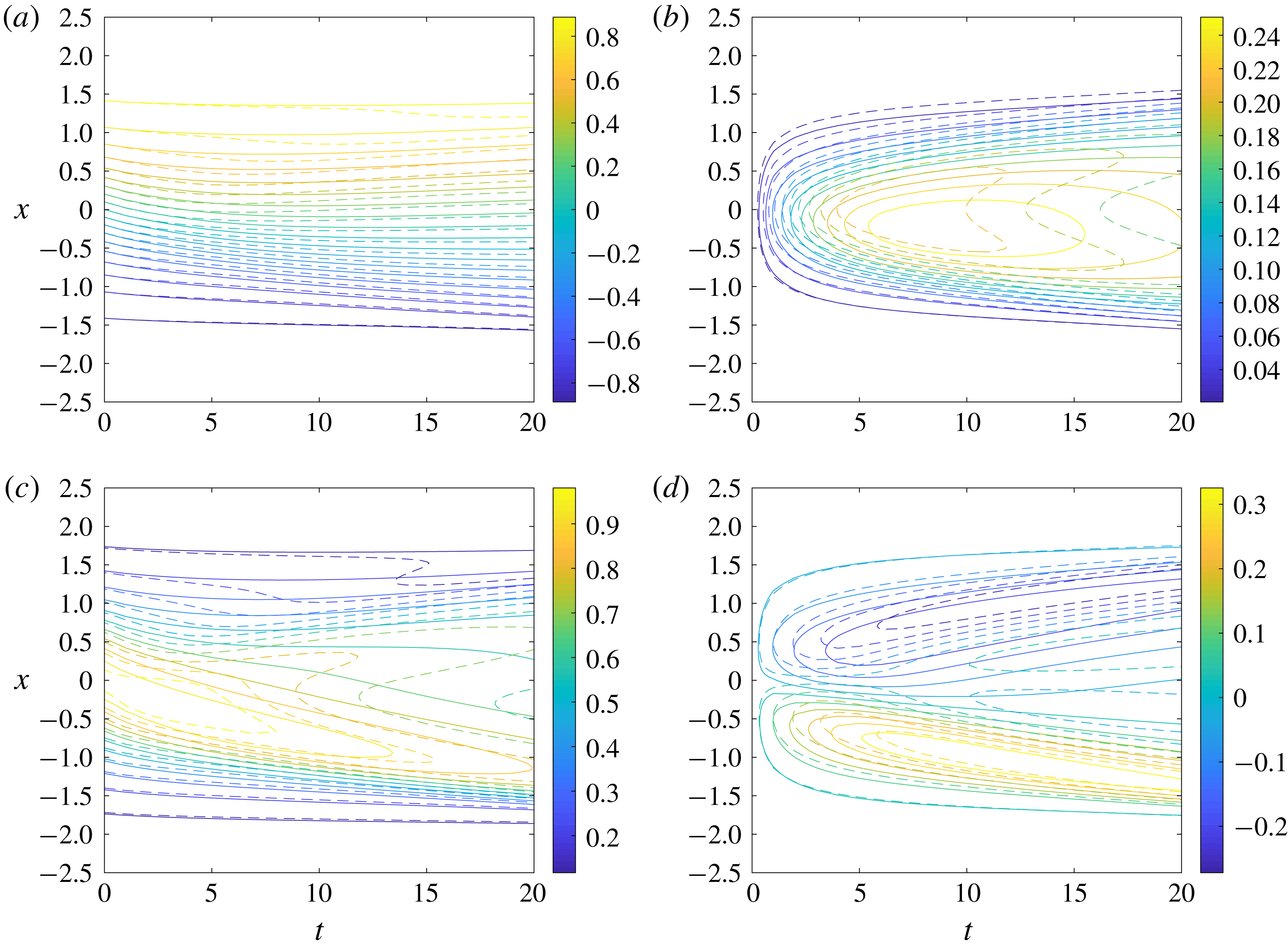
Figures 8 and 9 show the initial evolution of the surface buoyancy,
 $b(x,1/2,t)$
, and the surface buoyancy gradient,
 $M^{2}(x,1/2,t)$
for
 $Ro=1$
and
 $E=0.02,0.2$
. We also show the difference between the surface and centreline values of
 $b_{0}$
and
 $M^{2}$
since to leading order these correspond to
 $Ro\,b_{1}$
and
 $Ro\,\unicode[STIX]{x2202}b_{1}/\unicode[STIX]{x2202}x$
respectively. The analytic predictions to order
 $O(Ro)$
are shown by the dashed contours. We can see that the analytic predictions are fairly accurate for
 $E=0.02$
with a maximum error of approximately 25 % and very accurate for
 $E=0.2$
with a maximum error of approximately 2 %. In both cases the theory accurately predicts the time taken for the depth dependence to develop as well as both the position and the value of the maximum buoyancy gradient despite the Rossby number not being small and only using a prediction correct to first order in
 $Ro$
. If there are additional frontogentic mechanisms, such as an imposed strain flow, the increase in the surface buoyancy gradient can be large and the theory based on the assumption of small Rossby model will likely no longer be valid. In this case a more general model will be required (Shakespeare & Taylor Reference Shakespeare and Taylor2013; McWilliams Reference McWilliams2017; Sullivan & McWilliams Reference Sullivan and McWilliams2018).
5 Theory for
 $O(1)$
Rossby number and small Ekman number

As noted above, the largest differences between the theoretical predictions and numerical simulations occur for large
 $Ro$
and small
 $E$
. In this section we analyse the momentum budget to identify the source of these discrepancies. We then propose a modification to TTW balance that includes the influence of a depth-independent geostrophic flow. We use this to extend the theory in Crowe & Taylor (Reference Crowe and Taylor2018) to
 $O(1)$
Rossby numbers and small Ekman numbers and find that it leads to excellent agreement with the numerical simulations.
Plots of the terms in the horizontal momentum balances for
 $E=0.01$
and
 $Ro=0.1$
(a,b) and
 $Ro=1$
(c,d). Calculations use the data from our numerical simulations at
 $t=100$
and
 $x=0$
.

Figure 10 shows the balances in the horizontal momentum equations for
 $E=0.01$
and
 $Ro=(1,0.1)$
at
 $t=100$
and
 $x=0$
. We can see that the cross-front (
 $x$
) momentum equations in both cases are very close to TTW balance, even for
 $Ro=1$
. However, there are significant deviations in the
 $y$
momentum equation due to a large advection term. We find that
 $\text{D}v/\text{D}t$
is dominated by
 $u\,\unicode[STIX]{x2202}v/\unicode[STIX]{x2202}x$
with the along-front velocity,
 $v$
, developing a large depth-independent component corresponding to two jets of opposite direction as shown in figure 11.
In order to understand the formation of these jets, we can examine the depth-averaged along-front momentum equation. First, define the depth average as
 $$\begin{eqnarray}\overline{(\ast )}=\int _{-1/2}^{1/2}(\ast )\,\text{d}z,\end{eqnarray}$$
and write
 $(\ast )^{\prime }=(\ast )-\overline{(\ast )}$
to denote the deviation from this average. Depth averaging the
 $y$
momentum equation then gives
 $$\begin{eqnarray}Ro\left(\frac{\unicode[STIX]{x2202}\overline{v}}{\unicode[STIX]{x2202}t}+\frac{\unicode[STIX]{x2202}}{\unicode[STIX]{x2202}x}\overline{u^{\prime }v^{\prime }}\right)=\unicode[STIX]{x1D716}^{2}E\,\unicode[STIX]{x1D6FB}_{H}^{2}\overline{v},\end{eqnarray}$$
where we have assumed that
 $\overline{u}=0$
by symmetry (and hence
 $u^{\prime }=u$
). For
 $\unicode[STIX]{x1D716}^{2}E\ll Ro$
we can write
 $$\begin{eqnarray}\frac{\unicode[STIX]{x2202}\overline{v}}{\unicode[STIX]{x2202}t}=-\frac{\unicode[STIX]{x2202}}{\unicode[STIX]{x2202}x}\overline{u^{\prime }v^{\prime }},\end{eqnarray}$$
hence a depth-independent jet forms due to the correlation between the along-front and cross-front velocity fields. The cross-front velocity displaces the along-front thermal wind jets in the cross-front direction. This results in a cross-front flux of along-front momentum which accelerates the along-front flow in regions between the centre (
 $x=0$
) and frontal edges. This component of the along-front flow is mixed vertically on the fast time scale,
 $\unicode[STIX]{x1D70F}$
, leading to the formation of a depth-independent flow. For the initial condition considered here, the depth average of the along-front velocity is exactly zero. However, as the front evolves, this depth-independent flow can become large and acts to disrupt the TTW balance.
(a) Plot of
 $v(x,z)$
at
 $t=100$
. (b) Plot of
 $\overline{v}$
showing the structure of the depth-independent jet,
 $b_{0}$
is included for comparison.

Splitting the along-front velocity into depth-average and deviation quantities, we can write the horizontal momentum equations as
 $$\begin{eqnarray}Ro\frac{\text{D}u}{\text{D}t}-v^{\prime }-\overline{v}=-\frac{\unicode[STIX]{x2202}p}{\unicode[STIX]{x2202}x}+E\unicode[STIX]{x1D6FB}_{\unicode[STIX]{x1D716}}^{2}u\end{eqnarray}$$
and
 $$\begin{eqnarray}Ro\left(\frac{\text{D}v^{\prime }}{\text{D}t}+\frac{\unicode[STIX]{x2202}\overline{v}}{\unicode[STIX]{x2202}t}+u\frac{\unicode[STIX]{x2202}\overline{v}}{\unicode[STIX]{x2202}x}\right)+u=E\unicode[STIX]{x1D6FB}_{\unicode[STIX]{x1D716}}^{2}v.\end{eqnarray}$$
If we depth average equation (5.4) we find that the Coriolis term
 $-\overline{v}$
is balanced by the depth-independent component of the pressure gradient,
 $-\unicode[STIX]{x2202}\overline{p}/\unicode[STIX]{x2202}x$
, i.e. geostrophic balance. Hence
 $$\begin{eqnarray}Ro\frac{\text{D}u}{\text{D}t}-v^{\prime }=-\frac{\unicode[STIX]{x2202}p^{\prime }}{\unicode[STIX]{x2202}x}+E\unicode[STIX]{x1D6FB}_{\unicode[STIX]{x1D716}}^{2}u.\end{eqnarray}$$
Assuming that
 $u$
and
 $v^{\prime }$
remain order-1 fields, we have that
 $\unicode[STIX]{x2202}\overline{v}/\unicode[STIX]{x2202}t=O(1)$
by (5.3). However, we note that over the long time scale,
 $T=Ro\,t$
, we can have
 $\overline{v}=O(1/Ro)$
. Therefore the term
 $Ro\,u\,\unicode[STIX]{x2202}\overline{v}/\unicode[STIX]{x2202}x$
in (5.5) may appear in the leading-order balance.
If we now assume that
 $Ro$
is small, we obtain the leading-order velocity balance
 $$\begin{eqnarray}-v_{0}^{\prime }=-\frac{\unicode[STIX]{x2202}p_{0}^{\prime }}{\unicode[STIX]{x2202}x}+E\frac{\unicode[STIX]{x2202}^{2}u_{0}}{\unicode[STIX]{x2202}z^{2}}\end{eqnarray}$$
and
 $$\begin{eqnarray}\left(Ro\frac{\unicode[STIX]{x2202}\overline{v}}{\unicode[STIX]{x2202}x}+1\right)u_{0}=E\frac{\unicode[STIX]{x2202}^{2}v_{0}^{\prime }}{\unicode[STIX]{x2202}z^{2}},\end{eqnarray}$$
hence
 $\overline{v}$
is a background geostrophic flow which modifies the absolute vorticity of the system. We note that
 $\overline{v}$
will form spontaneously and evolve throughout time in contrast to the imposed geostrophic flow often used in frontal problems (e.g. Thomas & Lee (Reference Thomas and Lee2005)). Equations (5.7) and (5.8) are only asymptotically valid in the limit of small Rossby number, however, examining the momentum balances we find that this approximation is accurate outside the region of initial frontogenesis for all parameter values tested.
Equations (5.7) and (5.8) can be solved to obtain a modified TTW solution for the leading-order velocity
 $$\begin{eqnarray}\displaystyle & \displaystyle u_{0}=-\sqrt{\frac{E_{g}}{Ro\displaystyle \frac{\unicode[STIX]{x2202}\overline{v}}{\unicode[STIX]{x2202}x}+1}}\,K_{0}^{\prime \prime }\left(\frac{z}{\sqrt{E_{g}}};\frac{1}{\sqrt{4E_{g}}}\right)\frac{\unicode[STIX]{x2202}b_{0}}{\unicode[STIX]{x2202}x}, & \displaystyle\end{eqnarray}$$
 $$\begin{eqnarray}\displaystyle & \displaystyle v_{0}^{\prime }=-\sqrt{E_{g}}K_{0}\left(\frac{z}{\sqrt{E_{g}}};\frac{1}{\sqrt{4E_{g}}}\right)\frac{\unicode[STIX]{x2202}b_{0}}{\unicode[STIX]{x2202}x}, & \displaystyle\end{eqnarray}$$
 $E_{g}$
is the Ekman number modified by the geostrophic flow
 $$\begin{eqnarray}E_{g}=\frac{E}{\sqrt{Ro\displaystyle \frac{\unicode[STIX]{x2202}\overline{v}}{\unicode[STIX]{x2202}x}+1}}.\end{eqnarray}$$
The
 $O(Ro)$
buoyancy correction can now be calculated as
 $$\begin{eqnarray}b_{1}=-\frac{\sqrt{E_{g}}\,Pr}{Ro\displaystyle \frac{\unicode[STIX]{x2202}\overline{v}}{\unicode[STIX]{x2202}x}+1}K_{0}\left(\frac{z}{\sqrt{E_{g}}};\frac{1}{\sqrt{4E_{g}}}\right)\left[\frac{\unicode[STIX]{x2202}b_{0}}{\unicode[STIX]{x2202}x}\right]^{2},\end{eqnarray}$$
by the same steps described in Crowe & Taylor (Reference Crowe and Taylor2018). Combining our results, the background buoyancy field satisfies
 $$\begin{eqnarray}\frac{\unicode[STIX]{x2202}b_{0}}{\unicode[STIX]{x2202}T}=\frac{\unicode[STIX]{x2202}}{\unicode[STIX]{x2202}x}\left[\frac{E_{g}\,Pr}{\left(g_{0}+1\right)^{3/2}}\overline{K_{0}^{\prime 2}\left(\frac{z}{\sqrt{E_{g}}};\frac{1}{\sqrt{4E_{g}}}\right)}\left(\frac{\unicode[STIX]{x2202}b_{0}}{\unicode[STIX]{x2202}x}\right)^{3}\right],\end{eqnarray}$$
and from (5.3),
 $$\begin{eqnarray}\frac{\unicode[STIX]{x2202}g_{0}}{\unicode[STIX]{x2202}T}=\frac{\unicode[STIX]{x2202}^{2}}{\unicode[STIX]{x2202}x^{2}}\left[\frac{E_{g}}{\left(g_{0}+1\right)^{1/2}}\overline{K_{0}^{\prime 2}\left(\frac{z}{\sqrt{E_{g}}};\frac{1}{\sqrt{4E_{g}}}\right)}\left(\frac{\unicode[STIX]{x2202}b_{0}}{\unicode[STIX]{x2202}x}\right)^{2}\right],\end{eqnarray}$$
where
 $$\begin{eqnarray}g_{0}=Ro\frac{\unicode[STIX]{x2202}\overline{v}}{\unicode[STIX]{x2202}x}\end{eqnarray}$$
is the vertical vorticity associated with the depth-independent geostrophic flow and
 $E_{g}=E/\sqrt{1+g_{0}}$
. In the absence of a depth-independent flow
 $(\overline{v}=0)$
, equation (5.9) reduces to TTW balance. The expressions in (5.13) and (5.12) can therefore be viewed as a generalisation of the theory described in Crowe & Taylor (Reference Crowe and Taylor2018).
To test these predictions we compare the horizontal velocity fields from a range of simulations with both our original TTW predictions and our modified TTW solution from (5.9). The TTW and modified TTW solutions are calculated using
 $b_{0}$
and
 $g_{0}$
from the simulations. Figure 12 shows a comparison between the numerical cross-front velocity and our two analytic predictions; TTW balance and the modification to this balance given in (5.9). We can see that the modified TTW balance very closely matches the numerical profiles with a difference of less than 1 % in all cases. Since the balance described in (5.7) and (5.8) is found to be accurate, we conclude that the accuracy of our spreading rate predictions depends on how large the geostrophic flow becomes for each pair of parameters,
 $(Ro,E)$
.
Comparison of the cross-front velocity field between numerical simulations, TTW balance and the modified TTW balance (5.9) for (a)
 $Ro=0.1,E=0.01$
, (b)
 $Ro=1,E=0.01$
, (c)
 $Ro=0.1,E=0.1$
and (d)
 $Ro=1,E=0.1$
. The fields are evaluated at
 $x=0$
and
 $T=100$
.

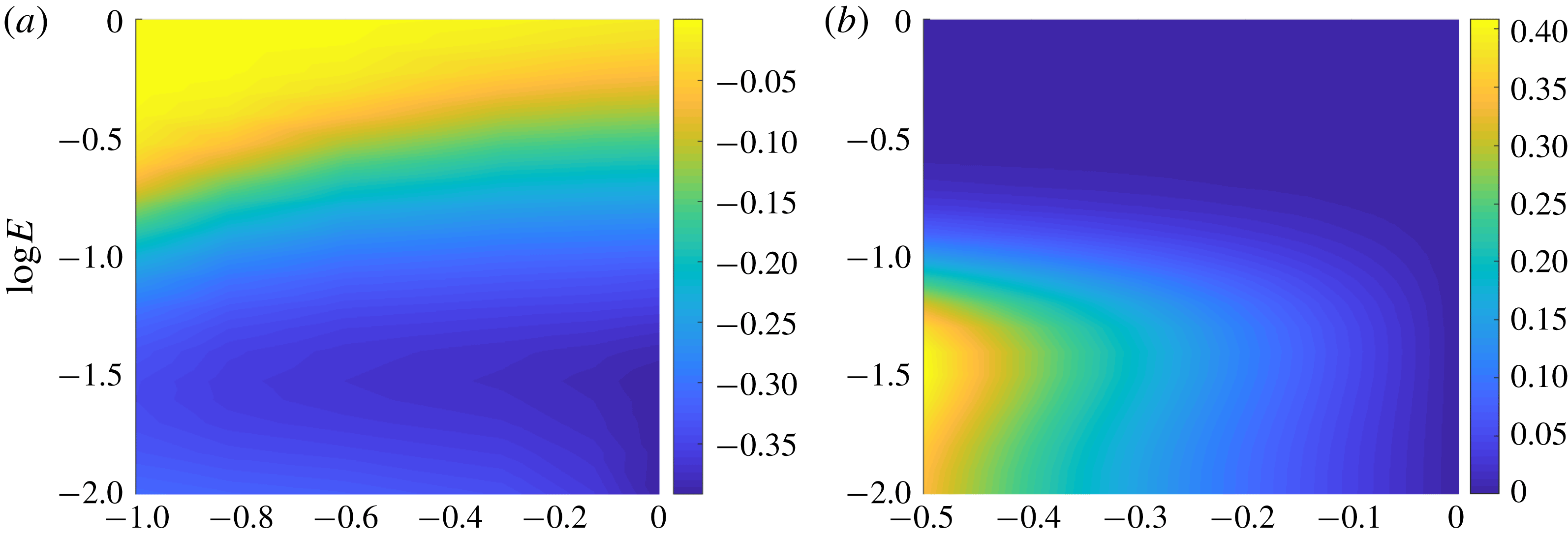
Figure 13(a) shows the magnitude of
 $g_{0}=Ro\,\unicode[STIX]{x2202}\overline{v}/\unicode[STIX]{x2202}x$
from our numerical simulations at
 $x=0$
and
 $T=100$
as a function of
 $E$
and
 $Ro$
. Figure 13(b) shows the maximum relative error between the TTW and modified TTW cross-front velocity (
 $u$
) solutions as a function of
 $E$
and
 $g_{0}$
. From figure 13(a) we can see that
 $g_{0}$
can become large for small values of
 $E$
. Hence, from figure 13(b), the magnitude of the cross-front velocity can change significantly – by approximately 30 % for
 $E<0.05$
. We note that even a large
 $g_{0}$
has very little effect on the cross-front velocity in the case of large
 $E$
. For large
 $E$
, the horizontal momentum balance is controlled by the dominant pressure gradient and vertical diffusion terms. Therefore the effect of changing the relative rotation is less significant than in the case of small
 $E$
where the horizontal momentum balance reduces to thermal wind balance between the pressure gradient and rotation term. Interestingly we do not see much variation with
 $Ro$
since both
 $g_{0}$
and
 $b_{0}$
evolve on the slow time scale
 $T$
and there remains no explicit
 $Ro$
dependence in (5.12) and (5.13). This is consistent with figure 13(a) where any weak
 $Ro$
dependence likely arises through
 $Ro$
dependent processes such as the time taken for the system to equilibrate and begin spreading via shear dispersion and the effects of horizontal diffusion.
(a) Value of
 $g_{0}$
determined from our simulation results at
 $T\,=\,100$
and
 $x\,=\,0$
as a function of
 $E$
and
 $Ro$
. (b) The maximum relative error between the TTW and modified TTW cross-front velocity fields (
 $u$
) as a function of
 $E$
and
 $g_{0}$
.

From (5.12) we can define a refined effective diffusivity function,
 $Q_{g}$
, by
 $$\begin{eqnarray}Q_{g}(x;E)=\frac{E_{g}}{(g_{0}+1)^{3/2}}\overline{K_{0}^{\prime 2}\left(\frac{z}{\sqrt{E_{g}}};\frac{1}{\sqrt{4E_{g}}}\right)},\end{eqnarray}$$
so (5.12) can be written as
 $$\begin{eqnarray}\frac{\unicode[STIX]{x2202}b_{0}}{\unicode[STIX]{x2202}T}=\frac{\unicode[STIX]{x2202}}{\unicode[STIX]{x2202}x}\left[Pr\,Q_{g}(x;E)\left(\frac{\unicode[STIX]{x2202}b_{0}}{\unicode[STIX]{x2202}x}\right)^{3}\right].\end{eqnarray}$$
We note that
 $Q_{g}$
has a complex dependence on
 $x$
and
 $T$
so (5.16) cannot be solved using a similarity solution. Figure 14 shows
 $g_{0}$
and
 $Q_{g}$
calculated from our numerical simulation for
 $E=0.01$
and
 $Ro=1$
. We can see that
 $g_{0}$
is negative throughout the middle of the frontal region corresponding to a higher effective diffusivity. At the frontal edges
 $g_{0}$
is strongly positive resulting in a decrease to the effective diffusivity.
Earlier, in the case of
 $g_{0}=0$
we found that the frontal width scales as
 $x\sim \unicode[STIX]{x1D6FE}T^{1/4}$
where
 $\unicode[STIX]{x1D6FE}\sim Q^{1/4}$
due to the nonlinear nature of the spreading. If we assume that the modified spreading parameter is
 $\unicode[STIX]{x1D6FE}_{g}\sim Q_{g}^{1/4}$
we find that the spreading rate is less sensitive to the effects of a geostrophic flow than the velocity fields due to the
 $1/4$
power dependence. Additionally, the spreading rate increases in the centre of the domain and decreases at the edges, therefore averaging
 $\unicode[STIX]{x1D6FE}_{g}$
across the domain gives a value very similar to the original predicted value of
 $\unicode[STIX]{x1D6FE}$
. Therefore we do not expect significant change in the spreading rate which is consistent with the accuracy of our original predictions in figure 3.
(a) Value of
 $g_{0}$
determined from our simulation results as a function of
 $x$
and
 $T$
for
 $E=0.01$
and
 $Ro=1$
. (b) Value of
 $Q_{g}(x,E)$
as a function of
 $x$
and
 $T$
for
 $E=0.01$
and
 $Ro=1$
;
 $Q_{g}$
is determined using (5.15) and
 $g_{0}$
from our simulations.

6 Scaling for vertical velocity
A distinguishing feature of the circulation around the front is the appearance of large vertical velocities at the edges of the front. This is visible in the streamfunction associated with the simulations and the theory for the case plotted in figure 4 through a bunching of the streamlines near
 $x=\pm 3$
. However, the theory described in Crowe & Taylor (Reference Crowe and Taylor2018) did not provide a prediction for the magnitude of the vertical velocity. In this section we will extend the theory to estimate the magnitude of the vertical velocity and the width of the regions of enhanced up/downwelling and test this prediction using the numerical simulations.
The theoretical prediction for the leading-order vertical velocity is
 $$\begin{eqnarray}w_{0}=E\,K_{0}^{\prime }(z/\sqrt{E})\frac{\unicode[STIX]{x2202}^{2}b_{0}}{\unicode[STIX]{x2202}x^{2}}.\end{eqnarray}$$
However, since our similarity solution for
 $b_{0}$
(4.2) is piecewise with infinite curvature (
 $\unicode[STIX]{x2202}^{2}b_{0}/\unicode[STIX]{x2202}x^{2}$
) at the frontal edges, the theory is unable to predict the strength of the up/down-welling that occurs at the edges of the front. Figure 15 shows the centreline values of the buoyancy and the vertical velocity for two different values of Rossby number. We can see than the maximum vertical velocity occurs at the edge of the front where the curvature is high and when the frontal edges are sharper (i.e. a greater curvature confined to a narrower region), the vertical velocity appears in thin bands of strong up/down-welling which correspond to the high curvature regions. We note that for
 $Ro=1$
these bands become very narrow and may be susceptible to numerical errors.
Plot of the centreline buoyancy (solid line) and centreline vertical velocity (dashed line) for
 $E=0.1$
and (a)
 $Ro=0.25$
, (b)
 $Ro=1$
at
 $T=200$
.

Though we cannot predict the functional form of
 $\unicode[STIX]{x2202}^{2}b_{0}/\unicode[STIX]{x2202}x^{2}$
and hence
 $w_{0}$
near the edges of the front from our analytic solution, we can use the similarity solution to estimate a scaling for the maximum vertical velocity. From Crowe & Taylor (Reference Crowe and Taylor2018) the buoyancy field,
 $b_{0}$
, is determined by the equation
 $$\begin{eqnarray}\frac{\unicode[STIX]{x2202}b_{0}}{\unicode[STIX]{x2202}T}=\frac{\unicode[STIX]{x2202}}{\unicode[STIX]{x2202}x}\left[Pr\,Q\left(\frac{\unicode[STIX]{x2202}b_{0}}{\unicode[STIX]{x2202}x}\right)^{3}+\frac{\unicode[STIX]{x1D716}^{2}E}{Ro^{2}Pr}\frac{\unicode[STIX]{x2202}b_{0}}{\unicode[STIX]{x2202}x}\right],\end{eqnarray}$$
where
 $Q(E)$
is defined in (4.8). The similarity solution arises as the solution of this equation when the second term in brackets is small, corresponding to an approximate balance between time evolution and shear dispersion. Near the edges of the front, where the curvature is high, the term describing horizontal diffusion becomes important and smooths out the singularity in
 $F^{\prime \prime }$
.
We now assume that there are thin regions at the edges of the front where this smoothing occurs. In these regions we assume that the horizontal diffusion term is similar in magnitude to the other two terms and the curvature of the front,
 $\unicode[STIX]{x2202}^{2}b_{0}/\unicode[STIX]{x2202}x^{2}$
, is approximately constant. Using the similarity solution we have that
 $$\begin{eqnarray}Pr\,Q\,\frac{\unicode[STIX]{x2202}}{\unicode[STIX]{x2202}x}\left(\frac{\unicode[STIX]{x2202}b_{0}}{\unicode[STIX]{x2202}x}\right)^{3}\sim -\frac{\unicode[STIX]{x1D702}}{4T}\sqrt{1-\frac{\unicode[STIX]{x03C0}^{2}\unicode[STIX]{x1D702}^{2}}{16}}\end{eqnarray}$$
and
 $$\begin{eqnarray}\frac{\unicode[STIX]{x1D716}^{2}E}{Ro^{2}Pr}\frac{\unicode[STIX]{x2202}^{2}b_{0}}{\unicode[STIX]{x2202}x^{2}}\sim -\frac{\unicode[STIX]{x1D716}^{2}E}{Ro^{2}Pr}\frac{\unicode[STIX]{x03C0}^{2}\unicode[STIX]{x1D702}}{16\unicode[STIX]{x1D6FE}^{2}T^{1/2}}\frac{1}{\sqrt{1-{\displaystyle \frac{\unicode[STIX]{x03C0}^{2}\unicode[STIX]{x1D702}^{2}}{16}}}}.\end{eqnarray}$$
Balancing these two terms gives that
 $$\begin{eqnarray}1-\frac{\unicode[STIX]{x03C0}^{2}\unicode[STIX]{x1D702}^{2}}{16}\sim \frac{\unicode[STIX]{x1D716}^{2}E}{Ro^{2}Pr}\frac{\unicode[STIX]{x03C0}^{2}T^{1/2}}{4\unicode[STIX]{x1D6FE}^{2}},\end{eqnarray}$$
and allows us to estimate the width of the smoothing regions by writing
 $$\begin{eqnarray}\unicode[STIX]{x1D702}=\pm \left(\frac{4}{\unicode[STIX]{x03C0}}-\unicode[STIX]{x1D712}\right)\end{eqnarray}$$
for small region width
 $\unicode[STIX]{x1D712}$
to get
 $$\begin{eqnarray}\unicode[STIX]{x1D712}\sim \frac{\unicode[STIX]{x1D716}^{2}E}{Ro^{2}Pr}\frac{\unicode[STIX]{x03C0}T^{1/2}}{2\unicode[STIX]{x1D6FE}^{2}}.\end{eqnarray}$$
When the edges spread to fill the whole domain we have
 $\unicode[STIX]{x1D712}\sim 1$
and recover the result from (4.6). We can now use (6.5) to estimate the magnitude of the curvature near the frontal edge (
 $\unicode[STIX]{x1D702}\approx \pm 4/\unicode[STIX]{x03C0}$
) as
 $$\begin{eqnarray}\frac{\unicode[STIX]{x2202}^{2}b_{0}}{\unicode[STIX]{x2202}x^{2}}\sim \mp \frac{Ro\sqrt{Pr}}{2\unicode[STIX]{x1D716}\unicode[STIX]{x1D6FE}\sqrt{E}\,T^{3/4}},\end{eqnarray}$$
and since
 $$\begin{eqnarray}w_{0}=E\,K_{0}^{\prime }\frac{\unicode[STIX]{x2202}^{2}b_{0}}{\unicode[STIX]{x2202}x^{2}},\end{eqnarray}$$
the maximum vertical velocity (occurring at
 $z=0$
) scales as
 $$\begin{eqnarray}w_{0}\sim \pm w_{s},\end{eqnarray}$$
where
 $$\begin{eqnarray}w_{s}=\frac{Ro\sqrt{Pr}\,C(E)}{\unicode[STIX]{x1D716}\,T^{3/4}}\end{eqnarray}$$
and
 $$\begin{eqnarray}C(E)=\frac{\sqrt{E}|K_{0}^{\prime }(0)|}{(12\unicode[STIX]{x03C0}^{2}Q)^{1/4}}.\end{eqnarray}$$
We can also predict that the width of the bands of enhanced vertical velocity scales as
 $$\begin{eqnarray}\unicode[STIX]{x1D6FE}\,T^{1/4}\unicode[STIX]{x1D712}\sim \unicode[STIX]{x0394}x_{w}=\frac{\unicode[STIX]{x1D716}^{2}E}{Ro^{2}Pr}\frac{\unicode[STIX]{x03C0}T^{3/4}}{2\unicode[STIX]{x1D6FE}}.\end{eqnarray}$$
Note that
 $T=Ro\,t$
so these results can also be written in terms of the time
 $t$
with a different Rossby number scaling. Using the asymptotic behaviour of
 $K_{0}^{\prime }$
and
 $Q$
shown in Crowe & Taylor (Reference Crowe and Taylor2018) we find that
 $$\begin{eqnarray}C(E)\sim \left\{\begin{array}{@{}ll@{}}E^{1/4},\quad & E\ll 1,\\ E^{-3/4},\quad & E\gg 1,\end{array}\right.\end{eqnarray}$$
so we expect the vertical velocity to be small for both very small and very large values of
 $E$
, assuming that the regions of high vertical velocity are still thin (
 $\unicode[STIX]{x1D712}\ll 1$
).
We now use the numerical results to test these predictions. There are, however, some limitations to the numerical solution due to the resolution. For large
 $Ro$
or small
 $E$
the regions of enhanced vertical velocity can become very narrow and if they are of a scale similar or smaller than the grid size,
 $\unicode[STIX]{x0394}x$
, the vertical velocity will likely not be accurate. We therefore consider the quantity
 $\unicode[STIX]{x0394}x_{w}/\unicode[STIX]{x0394}x$
when examining each simulation to see if the regions of strong vertical velocity are likely to be well resolved.
(a) Value of
 $\log [C(E)]$
as a function of
 $E$
, note that for small
 $E$
,
 $C\sim E^{1/4}$
and for large
 $E$
,
 $C\sim E^{-3/4}$
from (6.14). (b) Value of
 $\log [\unicode[STIX]{x0394}x_{w}/\unicode[STIX]{x0394}x]$
as a function of
 $E$
and
 $Ro$
for
 $T=200$
. The black curve is the contour
 $\unicode[STIX]{x0394}x_{w}/\unicode[STIX]{x0394}x=1$
.

(a) Value of
 $\log [\max w]$
diagnosed from the numerical solutions as a function of
 $E$
and
 $Ro$
at
 $T=200$
. (b) Value of
 $\unicode[STIX]{x1D6FC}_{w}$
as a function of
 $E$
and
 $Ro$
over the time interval
 $T\in [100,350]$
. The curves in white are (a)
 $T_{max}=2000$
and (b)
 $T_{max}=3500$
and the curves in black are contours of
 $\unicode[STIX]{x0394}x_{w}/\unicode[STIX]{x0394}x=1$
at (a)
 $T=200$
and (b)
 $T=100$
. We expect the theoretical predictions to be valid between the two curves.

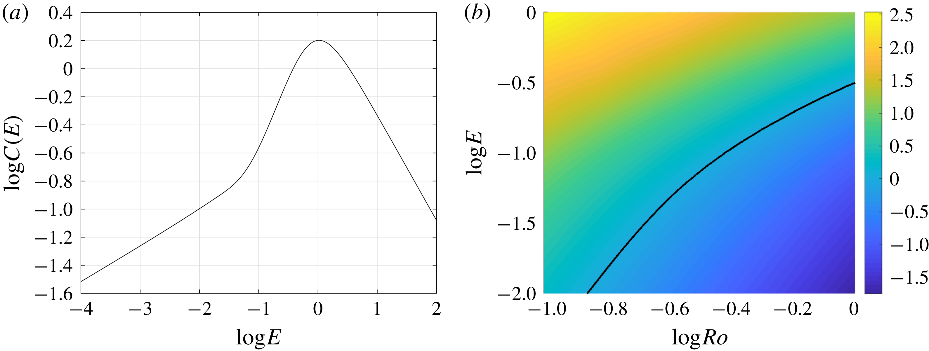
Figure 16(a) shows
 $C(E)$
as a function of the Ekman number,
 $E$
. The coefficient
 $C(E)$
and hence the vertical velocity are maximum for
 $E\simeq 1$
. Figure 16(b) shows the ratio of the predicted width of the region with enhanced vertical velocity to the horizonal grid spacing used in the simulations, i.e.
 $\log [\unicode[STIX]{x0394}x_{w}/\unicode[STIX]{x0394}x]$
. Here
 $\unicode[STIX]{x0394}x_{w}$
is calculated at
 $T=200$
. The black contour indicates
 $\unicode[STIX]{x0394}x_{w}/\unicode[STIX]{x0394}x=1$
. For all cases below this line, the grid spacing will be insufficient to capture the maximum vertical velocity.
Figure 17(a) shows the maximum vertical velocity at
 $T=200$
as diagnosed from the numerical simulations as a function of
 $E$
and
 $Ro$
. The curves in white show the region in which shear dispersion is dominant (the region below the curve) and the curves in black show the region where the regions of high curvature are smaller than the grid scale (the region below the curve). The theoretical prediction can be tested in the region between the white and black curves. The maximum vertical velocity increases with increasing
 $E$
for small
 $E$
and decreases with increasing
 $E$
for large
 $E$
. This is consistent with the predictions made in (6.11) since
 $C$
also has this behaviour. However, the maximum vertical velocity in the simulations is seen at
 $E\simeq 0.1$
while the theory predicts a maximum vertical velocity (and
 $C$
) at
 $E\simeq 1$
. The maximum vertical velocity diagnosed from the simulations increases approximately linearly with increasing
 $Ro$
, which is consistent with the theoretical prediction.
For larger Rossby numbers the effects of the
 $O(Ro)$
vertical velocity component may also become important and based on shape of the streamfunction from figure 4 we expect that the
 $O(Ro)$
vertical velocity will oppose the leading-order component and hence reduce the maximum up/down-welling. Since the leading-order streamfunction is still accurate for large
 $E$
(see figure 5
a), we can conclude that the effects of the
 $O(Ro)$
velocity component will be small for
 $E\gtrsim 0.1$
.
In order to determine the time dependence of the vertical velocity we fit
 $\max [w]$
to the curve
 $$\begin{eqnarray}\max [w]=\frac{\unicode[STIX]{x1D6FE}_{w}}{(T+T_{0})^{\unicode[STIX]{x1D6FC}_{w}}},\end{eqnarray}$$
to determine the value of the exponent,
 $\unicode[STIX]{x1D6FC}_{w}$
. Figure 17(b) shows the numerical values of the exponent calculated over a time interval of
 $T\in [100,350]$
, we can see that
 $\unicode[STIX]{x1D6FC}_{w}\approx 3/4$
in the region between the two curves where we expect the theory to be valid; this is in agreement with the predictions made in (6.11).
7 Conclusions and discussion
We have used fully nonlinear numerical simulations to consider the evolution of a front in the presence of strong vertical mixing, represented here through a large constant viscosity and diffusivity. As predicted in Crowe & Taylor (Reference Crowe and Taylor2018), vertical mixing induces spreading of the front via shear dispersion and the spreading rate diagnosed from the simulations agrees with the theory. The simulated velocity and buoyancy fields generally compare well with the theoretical predictions with a better agreement between the theory and simulations for larger Ekman numbers.
The accuracy of the theory seems to depend only weakly on the Rossby number and the theory is accurate even for
 $O(1)$
Rossby numbers despite the fact that the theory was based on an asymptotic analysis which was valid in the limit of small Rossby numbers. This can be explained by the Rossby number entering primarily through the formation of depth-independent geostrophic jets, the evolution of which do not explicitly depend on Rossby number. Interestingly, for
 $Ro=1,E=0.1$
, the theoretical prediction for the streamfunction is accurate to within 20 %, while the spreading rate is accurate to within about 5 %. It is not immediately apparent why the spreading rate is less sensitive to the formation of geostrophic jets than the velocity field though this may be a consequence of the functional dependence.
Despite the theory being derived for the TTW limit where the Ekman number is assumed to be order 1 and much larger than the Rossby number, we find that it is valid for a much larger range of
 $E$
with significant discrepancies only for
 $E=O(0.01)$
. For example we observe close (within
 $20\,\%$
) agreement between the theory and numerics when
 $Ro$
is one order of magnitude larger than
 $E$
. We have presented a refined theory which, while only asymptotically valid for small
 $Ro$
and large
 $E$
, accurately describes the evolution of the system and the formation of a depth-independent geostrophic jet for small
 $E$
and large
 $Ro$
. For larger Rossby numbers or smaller Ekman numbers the solution is driven away from TTW balance by nonlinear effects such as surface frontogenesis (McWilliams Reference McWilliams2017) and nonlinear Ekman transport (Stern Reference Stern1965; Niiler Reference Niiler1969; Thomas & Lee Reference Thomas and Lee2005). We note that the formation of a geostrophic jet requires frontal edges so only occurs in finite width fronts. Therefore our TTW solution is valid for the Garrett & Loder (Reference Garrett and Loder1981) case of small
 $E$
and
 $Ro$
examined in Crowe & Taylor (Reference Crowe and Taylor2018).
For
 $O(1)$
Rossby numbers and small Ekman numbers the adjustment from an initially depth-independent front can cause surface frontogenesis, although for the parameters considered here the increase in the horizontal buoyancy gradient is modest. In the absence of frictional and diabatic effects, other factors such as a background strain or unbalanced flow have been shown to sharpen fronts towards a discontinuity (Hoskins & Bretherton Reference Hoskins and Bretherton1972; Blumen Reference Blumen2000). It remains unclear whether a discontinuity could develop in response to TTW flow alone. For all Rossby numbers considered here, frontogenesis only occurs during a transient and eventually gives way to frontal spreading as predicted by the theory.
Finally, we derived a new scaling for the vertical velocity. This scaling agrees with the numerical simulations as long as the dominant balance in the buoyancy equation is between time dependence and shear dispersion (the horizontal diffusion is small) and the region of enhanced vertical velocity is sufficiently resolved in the numerical simulation.
A dimensional vertical velocity can be obtained from the theoretical prediction (
 $W=\unicode[STIX]{x0394}bH^{2}/(fL^{2})$
) using typical parameters for upper ocean fronts. For example, with
 $\unicode[STIX]{x0394}b=10^{-3}~\text{m}~\text{s}^{-2}$
,
 $H=100~\text{m}$
,
 $L=3~\text{km}$
and
 $f=10^{-4}~\text{s}^{-1}$
the vertical velocity scale is
 $W\,\approx \,10^{-2}~\text{m}~\text{s}^{-1}$
. Numerically we find that
 $w\sim 10^{-2}$
corresponding to a dimensional vertical velocity of
 $w^{\ast }\,=\,Ww\,\sim \,10^{-4}~\text{m}~\text{s}^{-1}$
or
 $10~\text{m}~\text{day}^{-1}$
. This prediction is of the same order of magnitude as vertical velocity diagnosed from ocean models (e.g. Mahadevan & Tandon (Reference Mahadevan and Tandon2006), Capet et al. (Reference Capet, McWilliams, Molemaker and Shchepetkin2008)), suggesting that the vertical circulation associated with turbulent thermal wind balance could contribute significantly to the vertical velocity at fronts.
The model presented in Crowe & Taylor (Reference Crowe and Taylor2018) and analysed here parameterises turbulent mixing through a depth-dependent viscosity and diffusivity. While this is very useful from a theoretical perspective, turbulence might not be well described by a viscous/diffusive closure. The assumption of a time-independent viscosity and diffusivity effectively decouples the influence of the front on turbulence. For example, in the limit of weak mixing, the slumping of the front can modulate the vertical density gradient, with stable stratification developing in some regions of the flow. This could suppress turbulence and the associated rate of vertical mixing (see e.g. Taylor & Ferrari (Reference Taylor and Ferrari2010)). Large-eddy simulations would be a useful tool to investigate details of the coupling between turbulence and the evolution of the front.
While the theory presented in Crowe & Taylor (Reference Crowe and Taylor2018) allowed for a three-dimensional front (including for example horizontal meanders), it neglects any non-TTW components of the flow. This prevents the development of baroclinic instability. Baroclinic instability and the resulting eddies extract potential energy from the front and cause the front to slump in the cross-front direction (e.g. Fox-Kemper, Ferrari & Hallberg (Reference Fox-Kemper, Ferrari and Hallberg2008)). A recent study by Bachman & Taylor (Reference Bachman and Taylor2016) investigated the combined effects of baroclinic instability and TTW-driven flow on the equilibrium stratification at a front. However, to our knowledge the evolution of an isolated front under the combined effects of baroclinic instability and TTW-driven shear dispersion has not been investigated.
The processes that act to broaden a front, including shear dispersion and baroclinic instability, can balance other processes acting to sharpen the front, ultimately controlling the frontal width. The frontal width (and hence the associated horizontal density gradient) is a crucial parameter for parameterisations of submesoscale processes (Fox-Kemper et al. Reference Fox-Kemper, Danabasoglu, Ferrari, Griffies, Hallberg, Holland, Maltrud, Peacock and Samuels2011; Bachman et al. Reference Bachman, Fox-Kemper, Taylor and Thomas2017). Since many fronts are under-resolved in global ocean and climate models, an improved description of the frontal width could lead to improved parameterisations of submesoscale processes.
Acknowledgements
The authors are grateful to three anonymous referees for helpful comments.