


Introduction
Maize is the most cultivated crop in Nigeria (FAO, 2018). In 2017, about 6.5 million hectares or 32% of the arable land in the country was allocated to maize, making Nigeria the leading African country in production area (FAO, 2018). Despite this large acreage, Nigeria is not the largest producer in Africa and it is not among the top 10 producers in the world (IITA, 2018). The average maize yield in the country is currently 1.8 tonnes ha−1 although yields of 7.5 to 10 tons have been reported in research stations and best farmer fields (NAERLS and FDAE, 2017). This low maize yield has been attributed to several reasons, encompassing edaphic, climatic, economic, and social factors (Badu-Apraku et al., Reference Badu-Apraku, Oyekunle, Obeng-Antwi, Osuman, Ado, Coulibaly, Yallou, Abdulai, Boakyewaa and Didjeira2012). The major factors limiting the yield of maize in Nigeria include the inherently poor soils (Jibrin et al., Reference Jibrin, Kamara and Ekeleme2012), frequent droughts and Striga infestations (Kamara et al., Reference Kamara, Ewansiha and Menkir2014), and low use of improved inputs such as fertilizers and seeds (Badu-Apraku et al., Reference Badu-Apraku, Oyekunle, Obeng-Antwi, Osuman, Ado, Coulibaly, Yallou, Abdulai, Boakyewaa and Didjeira2012). A serious but often overlooked reason is the lack of proper adherence to improved agronomic practices especially with respect to variety, appropriate planting dates, and selection of optimum sowing densities (Shaibu et al., Reference Shaibu, Adnan and Jibrin2016). The dramatic worldwide increase in per hectare grain yield of maize in the past 50 years has been attributed to the development of many specialty types of maize that are highly responsive to good agronomic practices (Mason and D’croz-Mason, Reference Mason and D’croz-Mason2002). Increased sowing density has been reported to be the agronomic practice with the largest contribution to this yield increase (Hashemi et al., Reference Hashemi, Herbert and Putnam2005; Liu and Tollenaar, Reference Liu and Tollenaar2009). Maize varieties currently released in Nigeria are bred and grown under relatively low plant density of 5.3 plants per m2, which is about half the sowing density adopted in countries with the highest maize grain yields per unit of land (NAERLS and FDAE, 2017). Sowing density recommendations for maize in Nigeria are low and most small-scale farmers plant even less than 50% of the recommended density due to lack of access to nitrogen (N) fertilizers (Muoneke et al., Reference Muoneke, Ogwuche and Kalu2007). A study has shown that the recommended sowing density could be increased without necessarily applying N fertilizers beyond the current recommendations (Kamara et al., Reference Kamara, Menkir, Kureh, Omoigui and Ekeleme2006).
Maize grain yields decrease with increasing sowing density beyond the optimum, but modern maize varieties are known to tolerate high densities even with low N application (O’Neill et al., Reference O’Neill, Shanahan, Schepers and Caldwell2004). Finding the best interactive function of adequate sowing density and N fertilizer application has been the focus of various studies (Al-Naggar et al., Reference Al-Naggar, Shabana, Mohamed and Tarek2015; Bhatt, Reference Bhatt2012; Qian et al., Reference Qian, Yang, Xiujie, Yubo, Yang, Zhongliang, Yubo, Liang, Zhenwei and Weijian2016). Stress caused by low N application frequently occurs with high sowing density conditions (Bänziger and Lafitte, Reference Bänziger and Lafitte1997). Because most farms in the maize belts of Nigeria have low inherent soil N contents and smallholder farmers face cash constraints to access expensive N fertilizers, it is important to provide sowing density management decisions for the low input and sub-optimal management conditions that are specific to fields and regional scales. Most studies on elevating maize sowing density in Nigeria report findings from on-station experiments under optimal management (Abubakar and Manga, Reference Abubakar and Manga2017; Kamara et al., Reference Kamara, Menkir, Kureh, Omoigui and Ekeleme2006; Muoneke et al., Reference Muoneke, Ogwuche and Kalu2007; Sani et al., Reference Sani, Oluwasemire and Mohammed2008). There is a need for research on maize sowing density and interaction with other management practices on farmers’ fields and if possible, incorporate the result of actual experiments to crop simulation models in order to have more spatial coverage and make better variety and location-specific recommendations for maize sowing density and N fertilizer recommendations.
Combining results from short-term experiments with robust, well-calibrated, and validated dynamic crop simulation models have been a common strategy for studying the effect of long-term climatic and edaphic variabilities while avoiding costly and time-consuming experiments (Holzworth et al., Reference Holzworth, Huth, deVoil, Zurcher, Herrmann, McLean, Chenu and Erik2014; Rezzoug et al., Reference Rezzoug, Gabreille, Suleiman and Benabdeli2008). The two most widely used models in Sub-Saharan Africa (SSA) are APSIM (Agricultural Production Systems Simulator) (Keating et al., Reference Keating, Carberry, Hammer, Probert, Robertson, Holzworth, Huth, Hargreaves, Meinke, Hochman, McLean, Verburg, Snow, Dimes, Silburn, Wang, Brown, Bristow, Asseng, Chapman, McCown, Freebairn and Smith2003) and DSSAT (Decision Support System for Agrotechnology Transfer) (Jones et al., Reference Jones, Hoogenboom, Porter, Boote, Batchelor, Hunt, Wilkens, Singh, Gijsman and Ritchie2003). The DSSAT suite incorporates different models for crops, soils, water, and climate simulations. CERES-Maize is one of the maize models in the DSSAT suite. It is a dynamic crop simulation model that estimates maize phenology, dry matter production/partitioning, and yield in daily time steps (Jones et al., Reference Jones, Kiniry and Dyke1986). The central core of the model is formed from routines set for estimating phenology and growth under non-limiting moisture and fertility conditions. Important processes simulated by the model include leaf initiation/growth, root/stem growth, light interception, timing of phenological phases, grain initiation and development, soil water extraction, transpiration, soil evaporation and N dynamics (Jones et al., Reference Jones, Hoogenboom, Porter, Boote, Batchelor, Hunt, Wilkens, Singh, Gijsman and Ritchie2003). The application of the CERES-Maize model to the SSA context is increasing. The model has recently been used to evaluate climate-sensitive farm management practices in the Northern Regions of Ghana (MacCarthy et al., Reference MacCarthy, Adiku, Freduah, Gbefo and Kamara2017), to identify appropriate sowing dates and N fertilizer rates in Zambia (Chisanga et al., Reference Chisanga, Phiri, Chizumba and Sichingabula2014), to simulate N and phosphorus (P) uptakes and soil moisture dynamics in West Africa (Amouzou et al., Reference Amouzou, Naab, Lamers and Becker2018), and to provide support for decision making for fertilizer micro-dosing for maize production in Benin (Tovihoudji et al., Reference Tovihoudji, Akponikpè, Agbossou and Bielders2019). Specifically for Nigeria, the model was used to determine the N fertilizer requirements of early maturing maize in the Sudan Savanna and the optimum planting dates in Northern Nigeria (Adnan et al., Reference Adnan, Jibrin, Kamara, Abdulrahman, Shaibu and Garba2017a, Reference Adnan, Jibrin, Kamara, Abdulrahman and Shaibu2017b), and to identify potential zones for maize production in South Western Nigeria (Iyanda et al., Reference Iyanda, Pranuthi, Dubey and Tripathi2014).
The strengths and limitations of the CERES-Maize model, particularly with respect to sowing density effects in Nigeria, have been documented in a seminal study in South-West Nigeria 21 years ago (Jagtap et al., Reference Jagtap, Alabi and Adeleye1998). This study analyzed the response of maize to different row arrangements/densities and tested the ability of the model to simulate the development, growth, and yield of maize over a range of planting densities. The study concluded that the maize variety did not respond to planting density beyond 6.9 plants m−2 and N fertilizer application beyond 75 to 100 kg ha−1 because of the genetic makeup of the variety. The authors also suggested that the use of the CERES-Maize model may show limitations due to the inaccessibility of soil and weather data, but most importantly due to lack of detailed crop data for calibrating the genotype-specific parameters (GSPs) of different varieties. The study opined that upon the development of high yielding varieties with upright leaf orientation and greater response to applied N. Having initially calibrated GSPs of 26 modern maize varieties reported to be tolerant to high sowing density (Adnan et al., Reference Adnan, Diels, Jibrin, Kamara, Craufurd, Shaibu, Mohammed and Tonnang2019), the current research was conducted with the following objectives: (i) calibrate CERES-Maize model using data collected from researcher managed experiments conducted in farmers’ fields with varying management conditions in two contrasting environments; (ii) evaluate the ability of the model to simulate the effect of elevated sowing density on different maize varieties used in Nigeria and sub-Saharan Africa; (iii) use the calibrated and validated model in making recommendations for optimum sowing density and N fertilizer application of maize in two contrasting environments; and (iv) determine the economic profitability of different management scenarios of maize in the SS and NGS.
Materials and Methods
Study locations and experimental set-up for model calibration and evaluation
Field trials were set-up in three Local Governments Areas (LGAs) each in the SS and NGS of the Nigerian maize belt during the rainy seasons of 2016 and 2017. In the SS, the trials were set up in 30 farmers’ fields (10 in each LGA) in Kura (N 11.78427 E 8.51331), Garun Mallam (N 11.66098 E 8.38254), and Bunkure (N 11.68318 E 8.52469). In the NGS, the 30 farmers’ fields were in Doguwa (N 10.72944 E 8.57747), Lere (N 10.52005 E 8.47313), and Ikara (N 11.14017 E 8.23507). In each of these locations, farmers were purposively selected to cover the different farmer groupings used by the Sasakawa Africa Association (SAA) extension programs. SAA farmers are grouped into five distinct classes (A–E) based on how long they have been in the program. Across locations, two farmers were randomly selected from each of these five groups. Class A and B farmers are the best-farmer class where fields are optimal and proper agronomic management decisions are practiced, especially for timely weeding. The remaining farmers are relatively new in the extension program and thus fields are not as optimal as class A and B. The same farmers and fields selected in 2016 were maintained and used in 2017.
The treatments consisted of 10 maize varieties of varying maturity levels (five early and five extra-early varieties in the SS and two early, two intermediate, and six late varieties in the NGS). The results from four varieties, one from each maturity group, were selected and are presented in this study. The varieties were planted at three sowing density levels: the national recommendation (5.33 plants m−2), 50% lower (2.66 plants m−2) and 20% higher (6.66 plants m−2). The density selection was done to capture the reality of sowing densities currently found in farmers’ fields (2.66 and 5.33 plants m−2) and a slight increase (6.66 plants m−2) over the recommendation. The densities were achieved by maintaining the same inter-row spacing (0.75 m) and then varying the intra-row spacing. For 2.66 plants m−2, an intra-row spacing of 0.5 m was used; for 5.33 plants m−2 0.25 m; and for 6.66 plants m−2 0.20 m. For each density, two plants were sown per hole and then thinned to one plant per hole 2 weeks after sowing. Sowing was carried out in each farmer’s field as soon as the rains were established based on the recommended sowing window in each agroecology. In 2016, there was a late establishment of rains and sowings were done on 20th June in Doguwa, 21st June in Ikara, and 24th June in Lere. In 2017, the fields in Doguwa were sown on 31st May while Ikara and Lere were sown on 2nd and 4th June, respectively. Fertilizer application was according to the regional recommendation (120N:60P2O5:60K2O kg ha−1); potassium (K) was applied as muriate of potash, P as single super phosphate, and N was applied as urea. While all the P and K fertilizers were applied at sowing, only half of the N fertilizer was applied at sowing (via incorporated band row placement) and the other half 21 days later. Each farmer field was planted with 10 plots, ensuring that all 10 varieties are sown together with random combinations of the three sowing densities according to the experimental design. The individual plot size was 30 m2 (eight ridges of 0.75 × 5 m length) and the net plot size was 12 m2 (4 × 4 m inner ridges). Data from the best farmer fields (class A and B), the recommended sowing density (5.3 plants m−2) and two recommended varieties (SAMMAZ 32 and SAMMAZ 41 in SS and SAMMAZ 15 and OBA SUPER 9 in NGS) in 2016 and 2017 were used for model calibration. Data from the remaining farmers (class C D and E) and the low and high sowing densities in 2016 and 2017 were used for model evaluation.
Experimental design and statistical analyses
The trials involved a full factorial design of 10 varieties and 3 densities implemented in 30 incomplete blocks. The blocks were the 30 farmers’ fields, that each had 10 experimental plots. The treatment combinations were allocated to the blocks using the design of experiment (DOE) platform of JMP version 13 software (SAS, 2018). The model was designed according to the D-optimality criterion (de Aguiar et al., Reference de Aguiar, Bourguignon, Khots, Massart and Phan-Than-Luu1995) with variety, the experience of a farmer, density, density*density, variety*density and variety*density*density as fixed effects while farmer (=block) and year were random factors. All measured variables were explored with an analysis of variance using a linear mixed model. The random effect of farmers was nested in both LGAs and years in the analyses. Main effects of year, sowing density, and variety together with their second-order interactions were estimated.
Model description
The CSM CERES-Maize model of DSSAT version 4.7.5 (Hoogenboom et al., Reference Hoogenboom, Porter, Boote, Shelia, Wilkens, Singh, White, Asseng, Lizaso, Moreno, Pavan, Ogoshi, Hunt, Tsuji and Jones2019) was used in this study. In the present study, the daily canopy photosynthesis method was used to simulate maize photosynthesis (Jones et al., Reference Jones, Kiniry and Dyke1986); the CENTURY model (Gijsman et al., Reference Gijsman, Hoogenboom, Parton and Kerridge2002) was used to simulate organic C (carbon) and N dynamics; the Priestly and Taylor (Priestly and Taylor, Reference Priestly and Taylor1972) method for evapotranspiration; and the Soil Conservation Service method (USDA-Soil Conservation Service, 1972) was used to simulate soil water infiltration.
Model parametrization
The major physiological processes (photosynthesis, respiration, accumulation, and partitioning of assimilates) in the CERES-Maize model are governed by six genetic coefficients. For the present calibration, GSPs of four already calibrated varieties (two for SS and two for NGS) were collected from Adnan et al. (Reference Adnan, Diels, Jibrin, Kamara, Craufurd, Shaibu, Mohammed and Tonnang2019). Required crop genetic inputs for CERES-Maize are given in Table 1 and they describe the growth, phenology, and yield characteristics according to varietal differences. The GSPs were not re-calibrated for the environments in the current study because the original calibration of the GSPs was done in the same environments.
Calibrated genotype-specific parameters of various maize varieties

P1, Thermal time from seedling emergence to the end of juvenile phase.
P2, Delay in development for each hour that day-length is above 12.5 hours.
P5, Thermal time from silking to time of physiological maturity.
G2, Maximum kernel number per plant.
G3, Kernel growth rate during linear grain filling stage under optimum conditions.
PHINT, Thermal time between successive leaf tip appearance.
In each experimental location before planting, soil pits were dug and soil samples were collected from each layer. The pH, texture, moisture, bulk density, exchangeable potassium (K), organic matter, P, total N, and CEC contents of the soil samples were determined. For the detailed calibration and validation experiments, daily weather data were collected from weather stations (Watchdog 2000 Series, Spectrum Technologies) adjacent to all experimental sites. Daily records of minimum and maximum temperature, total solar radiation, and total rainfall are required for the CERES-Maize model weather initialization. The Weatherman utility in DSSAT was used to create the weather file used by the CERES-Maize model. Soil data tool (SBuild) was used to create the soil database used for general simulations. Name of the country, name of experimental site, site code, site coordinates, soil series, and classification were entered in this utility. The coefficient, SLPF (soil fertility factor), was adjusted to capture the variations due to edaphic differences across locations.
Model calibration
Data on grain yield, biomass at harvest, number of days to maturity, and harvest index from the best farmer fields from the recommended sowing density (5.3 plants m−2) in 2016 and 2017 experiments in the three LGAs for each agroecology (2 farmers’ fields, 2 varieties, 2 years and 3 LGAs) were used for model calibrations. Separate calibrations were done for the SS and NGS agroecological zones. The DSSAT model inputs include cultivar coefficients, weather records (minimum and maximum temperature, rainfall, and relative humidity), initial soil moisture, soil organic C, N and soil inorganic N and P, soil topography/surface information, such as slope, soil color, and crop management details (Jones et al., Reference Jones, Hoogenboom, Porter, Boote, Batchelor, Hunt, Wilkens, Singh, Gijsman and Ritchie2010).
The target of the calibration process was to minimize RMSE (Ritter and Muñoz-Carpena, Reference Ritter and Muñoz-Carpena2013):
 $$RMSE = \sqrt {{{{{\sum\nolimits_{i = 1}^n {\left( {{m_i} - {s_i}} \right)} }^2}} \over n}} $$
and normalized RMSE (RMSEn) (Yang et al., Reference Yang, Yang, Liu and Hoogenboom2014):
 $$RMSEn = {{RMSE \times 100} \over {\overline m }}$$
Where n is the number of observations,
 ${{s_i}}$
is the simulated data,
 ${{m_i}}$
is the measured data, and
 $\overline m $
is the mean of the measured data. RMSE and RMSEn were used to compare simulated and measured values; model accuracy was considered very high if RMSEn was <10%, high if it is between 10 and 20%, moderate when it’s between 20 and 30%, and low when it is >30% as suggested by Jamieson et al. (Reference Jamieson, Porter and Wilson1991).
Model evaluation
The calibrated model was evaluated using data from all tested sowing densities in the remaining calibration exercise, and the evaluation was done separately for SS and NGS. Data for grain yield, harvest biomass, and days to physiological maturity from farmer fields with detailed soil profile data (four farmers out of six) in 2016 and 2017 were used for model evaluation. In addition to RMSE and RMSEn, the modeling efficiency (EF) was calculated using the formula of Yang et al. (Reference Yang, Yang, Liu and Hoogenboom2014):
 $$EF = {{{{\sum\nolimits_{i = 1}^n {\left( {{m_i} - \overline m } \right)} }^2} - {{\sum\nolimits_{i = 1}^n {\left( {{s_i} - \overline m } \right)} }^2}} \over {\sum\nolimits_{i = 1}^n {{{\left( {{m_i} - \overline m } \right)}^2}} }}$$
The modified index of agreement (modified d) was calculated according to Pereira et al. (Reference Pereira, Meschiatti, Matos and Blain2018)
 $$Modified\,d = 1 - {{\sum\nolimits_{i = 1}^n {\left| {{m_i} - {s_i}} \right|} } \over {\sum\nolimits_{i = 1}^n {{{\left( {\left| {{s_i}} \right| + \left| {{m_i}} \right|} \right)}^2}} }}$$
The values of EF range from −∞ to 1 and that of modified d ranges between 0 and 1 (for both, the higher the value the better). EF values between 0 and 1 are acceptable, while values ≤0 show a lack of agreement (Yang et al., Reference Yang, Yang, Liu and Hoogenboom2014). The parameter d is dimensionless and a value of 1 indicates a good agreement between observed and measured data, while 0 indicates no agreement (Moriasi et al., Reference Moriasi, Arnold, Van Liew, Bingner, Harmel and Veith2007). The modified d index was used instead of the actual d index (Willmott et al., Reference Willmott, Ackleson, Davis, Feddema, Legates, O’Donnell and Rowe1985) because in the modified d index, the errors and differences are given their appropriate weighting (Legates and McCabe, Reference Legates and McCabe1999).
A sensitivity analysis to test for the effect of elevated density was conducted after calibrating and evaluating the model. The analyses were done using soils from the best farmer fields in SS and NGS and using observed weather records for the year 2017. Recommended N fertilizers for early/extra early maize (90 kg N ha−1) and intermediate/late (120 kg N ha−1) maturing maize were adopted. The purpose of the sensitivity analyses was to confirm the model calibration and evaluation and check if the model can simulate conditions that were not used in the calibration and evaluation exercise. The early and extra-early varieties were tested in the SS while the intermediate and two late varieties were tested in the NGS. Planting density was increased by two plants m−2 starting from 4 plants to 14 plants m−2. Grain yields were simulated for each variety at the different planting densities.
Model application: Long-term seasonal analyses
The calibrated and evaluated CERES-Maize model was then used to assess the response of maize varieties to different sowing density-based management decisions in the maize belts of Northern Nigeria. Planting density, varietal selection, and N fertilization were simulated. The following set-up was used in the seasonal analyses tool for the long-term simulations:
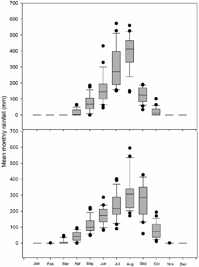
Long-term weather data (1992–2017) were collected from the Nigerian Meteorological Agency (NIMET) for Bunkure (representing Sudan savanna) and Zaria (representing wet savanna). Box plots showing the rainfall data are depicted in Figure 1. Data on rainfall, maximum and minimum temperatures, and solar radiation were used. Data for the selected locations and periods were used because they represent the range of conditions in maize-growing areas in Nigeria. The long-term simulations were done on a Typic Kanhaplustalf from Bunkure representing the SS and a Typic Kandiustalf from Samaru to represent the NGS. N, soil water content, and organic matter content were allowed to be carried over between seasons, thereby not necessitating re-initialization. Following typical farmers’ traditions in the study area, all residues were removed on the 1st of April in each year.
Records of 26 years rainfall data for the Sudan Savanna (upper panel) and Northern Guinea Savanna (lower panel).

For each simulation year, sowing was set to start when a total rainfall exceeding 20 mm occurred within the previous 3 days between June 1 to July 1 in the NGS and between June 10 to July 10 in the SS. The selected periods capture the normal sowing windows for maize in the study area (Kamara et al., Reference Kamara, Ekeleme, Chikoye and Omoigui2009). Four maize varieties, SAMMAZ 41, SAMMAZ 32, SAMMAZ 15 and Oba Super 9, were used which represent the extra-early, early, intermediate, and late maturity groups, respectively. The model was set to harvest when the crop reached harvest maturity.
Twelve standard scenarios were created by combining four sowing densities (2.6, 5.3, 6.6, and 8.8 plants m−2) with three N rates (30, 60, and 90 [120 in NGS] kg N ha−1). In each agroecology, the 12 scenarios (low-density low N [LDLN], low-density medium N [LDMN], low-density high N [LDHM], medium-density low N [MDLN], medium-density medium N [MDMN], medium-density high N [MDHN], high-density low N [HDLN], high-density medium N [HDMN], high-density high N [HDHN], very high-density low N [VHDLN], very high-density medium N [VHDMN], and very high-density high N [VHDHN]) were simulated using the two varieties adapted to that agroecology. For all simulated scenarios, the model was set up to apply N fertilizers in two equal splits, half at sowing and the other half at 3 weeks after sowing (conditions were set to postpone the second dose until the moisture conditions were sufficient in the rainfed scenarios). P and K were assumed to be non-limiting, so P and K sub-models were switched off. The planting densities were done by setting a constant inter-row spacing of 0.75 m and changing the intra-row spacing to meet the different density scenarios. Intra-row spacings of 0.15, 0.20, 0.25, and 0.50 m were adopted to provide the selected sowing densities of 8.8, 6.6, 5.3, and 2.6 plants m−2 respectively. Among the selected densities, 2.6 plants m−2 is used commonly by farmers especially at low fertilization, while 5.3 plants m−2 is the national recommendation. Findings by Kamara et al. (Reference Kamara, Menkir, Kureh, Omoigui and Ekeleme2006) indicate that modern maize cultivars could be planted with higher densities in the Nigerian savannas as long as adequate N fertilizer management is adopted. The irrigation and water management module in the model was set to automatic irrigation when required for the rainfed + supplementary irrigation scenarios.
An economic profitability analysis was performed using the economic and risk analysis tool of DSSAT. To set up the economic analysis requirements, historic market price data (2004–2017) of maize were collected for the SS and NGS from the Famine Early Warning Systems Network (FEWSNET) data repository (USAID, 2019). Input cost data, including labor and base production costs, were collected from 3 years (2015–2017) survey data conducted in the study areas (unpublished, Center for Dryland Agriculture). All nominal price data were adjusted for inflation to real price data by dividing the nominal price of an item (input or output variable) by the consumer price index (CPI). Historical market price data were also compounded to current price levels in order to have a single price of both inputs and outputs across years of simulations in the analyses. Simulated net revenue per unit of land (money ha−1) and per unit of family labor (not including hired labor) for each scenario were calculated. The labor cost per hectare for each household was converted to an adult equivalence scale using the modified OECD scale (Litchfield, Reference Litchfield1999).
Results
Climatic conditions across locations during experimental years
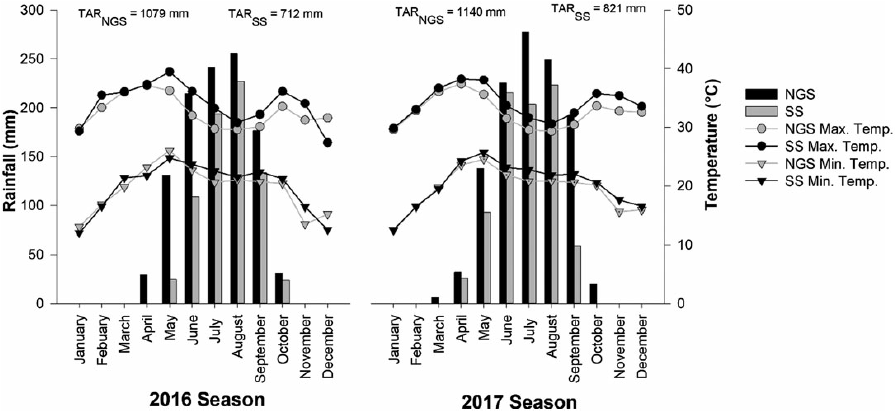
The total monthly rainfall and mean monthly minimum and maximum temperature for the three LGAs in NGS and SS are shown in Figure 2. The amount and distribution of rainfall during the experimental periods were different between the two seasons and the agro-ecologies. Higher rainfall was recorded in 2017 (1140 mm in NGS and 821 mm in SS) than in 2016 (1079 mm in NGS and 712 mm in SS). In 2016, an average of 93 and 68 rainy days was recorded in the three locations across the NGS and SS. In 2017, however, 115 and 82 rainy days were recorded in the NGS and SS respectively. Maximum average daily temperatures of 32.5 and 33.9 °C were recorded in the NGS and SS in 2016. While in 2017, the maximum temperatures were 33.9 and 34.1 °C in the NGS and SS. In the NGS, the average minimum daily temperatures were 19.3 °C in 2016 and 19.4 °C in 2017. In the SS, average minimum daily temperatures of 19.7 and 20.2 °C were recorded in 2016 and 2017.
Records of monthly rainfall (bars) and minimum and maximum temperatures (lines and markers) for the Northern Guinea Savanna (NGS) and the Sudan Savanna (SS) in 2016 and 2017. TAR = Total Annual Rainfall.

Model evaluation
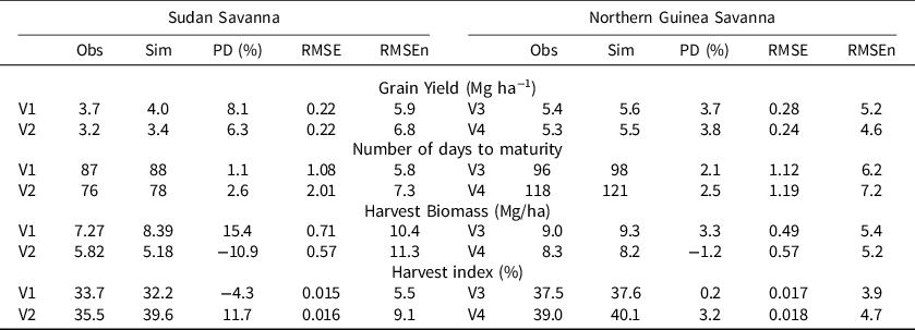
Observed and simulated grain yields, biomass at harvest, number of days to physiological maturity, and harvest index were compared for the different varieties across locations in 2016 and 2017 (Table 2). The GSPs used in the present study are shown in Table 1. The range of GSPs were close to the default generic parameters for very short (SAMMAZ 41), short (SAMMAZ 32), medium (SAMMAZ 15), and long (OBA super 9) season varieties in the DSSAT genotype files. In the SS, the model predicted grain yield and number of days to maturity of both varieties very accurately with prediction deviations (PD) below 7% and RMSEn below 8%. For harvest biomass and harvest index, the model predictions were good for both varieties with prediction deviations (PDs) below 15% and RMSEn below 12% for biomass and below 10% for harvest index. In the NGS, all measured parameters were also predicted very accurately for both varieties as evidenced by PDs below 5% and RMSEn below 8%. In both environments and for all varieties, the model predicted phenology (no of days to physiological maturity) more accurately than grain yield, biomass, and harvest index. The latter had the lowest accuracy.
Comparisons of observed and simulated grain yield, number of days to maturity, harvest biomass and harvest index for model calibrations in the Sudan Savanna and Northern Guinea Savanna

V1 = Sammaz 32, V2 = Sammaz 41, V3 = Sammaz 15, V3 = Oba Super 9.
PD, Prediction Deviations (negative values indicate under-simulation).
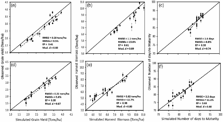
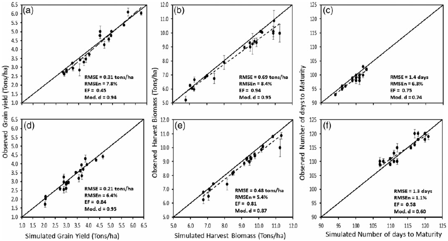
Comparisons between measured and simulated grain yield, biomass at harvest, and number of days to physiological maturity are shown in Figure 3 (A–F) for the SS and Figure 4 (A–F) for the NGS. The model predicted grain yields well for all the varieties in both agro-ecologies with RMSE values ranging between 0.21 and 0.34 tons ha−1, modified d index values ranging between 0.88 and 0.96, model efficiency values ranging between 0.39 and 0.84, and nRMSE values below 10% in all measurements. Evaluation of above-ground biomass at harvest was not as accurate as that of grain yield especially for the two varieties in the SS. For the variety SAMMAZ 32 (Figure 3B), model evaluation statistics were lowest (RMSE = 1.1 tons ha−1, RMSEn = 15%, EF = 0.61, and mod. d = 0.89) among all the evaluations. The variety Oba Super 9 had the best model evaluation statistics for biomass yield with RMSE value of 0.48 tons ha−1, EF of 0.81, modified d index value of 0.87, and RMSEn of 5.4%. Evaluation of the number of days to maturity was highly accurate for the two varieties in the NGS and SAMMAZ 32 in the SS. For SAMMAZ 41 in the SS, the model was just accurate with RMSE values of 2.2 days, EF of 0.53, and RMSEn of 11.1%. Overall, the model evaluation statistics were within acceptable ranges for all varieties across the two agro-ecologies. The model simulations showed no N stress for both years across all treatments. Dry spells were experienced around 38 to 42 and 66 to 73 days after sowing in all three locations of the SS in 2016. The model accurately simulated the observed moisture stress in two of the three locations (data not shown).
Observed vs simulated grain yields, harvest biomass, and number of days to physiological maturity for Sammaz 41 (A, B, and C) and Sammaz 32 (D, E and F) maize varieties for model validation data in the Sudan Savanna.

Observed vs simulate grain yields, harvest biomass, and number of days to physiological maturity for Sammaz 15 (A, B and C) and Oba Super 9 (D, E and F) maize varieties for model validation data in the Northern Guinea Savanna.

Sensitivity analyses
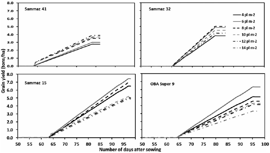
The result of the sensitivity analyses for the four varieties is shown in Figure 5. For SAMMAZ 41, grain yield was very sensitive to the increase in the number of plants m−2. A linear increase in grain yields was recorded with increasing sowing density up to 12 plants m−2 while a further increase to 14 plants m−2 resulted in yield decline. The yield differences between 8, 10, and 12 plants m−2 were negligible. For SAMMAZ 32, however, the highest grain yields were simulated for eight plants m−2 followed by six plants m−2 while four plants m−2 produced the lowest grain yield. The intermediate and late varieties produced higher grain yields with lower planting densities, for both varieties, the highest grain yields were simulated with sowing density of 6 plants m−2; however, for OBA Super 9, sowing density of 6 plants m−2 produced the highest grain yield followed by 4 plants m−2 while the variations between sowing densities of 8, 10, and 12 plants m−2 were not high.
Sensitivity analyses of calibrated and evaluated models for Sammaz 41 and Sammaz 32 (Sudan Savanna) and Sammaz 15 and Oba Super 9 (Northern Guinea Savanna) maize varieties, under different plant densities (4 to 14 plants per m2 [pl m−2]).

Model application
Sowing density scenarios
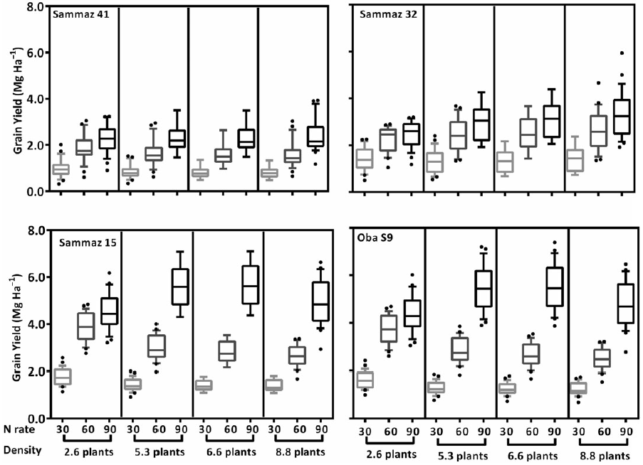
In the SS, consistent yield increases were observed with increasing planting density up to 8.8 and 6.6 plants m−2 for SAMMAZ 41 and SAMMAZ 32, respectively (Figure 6). The yield increase existed only when the increase in density is followed by a subsequent increase in N fertilizer application. The magnitude of yield increase with the addition of N fertilizers was also density-dependent. For instance, looking at SAMMAZ 41, average grain yield increased by 53.4% when N fertilizers were increased from 30 to 60 kg N ha−1 and only to 63.3% when further increased to 90 kg N ha−1 for the lowest sowing density (2.6 plants m−2). For medium sowing density (6.6 plants m−2), a yield increase of 87% was observed when N was increased from 30 to 60 while for high sowing density (8.8 plants m−2), a yield increase of 140% was observed when N was increased from 60 to 90 kg N ha−1. For the varieties in the NGS, consistent yield reductions were observed when sowing density was increased for low (30 kg N ha−1) and medium (60 kg N ha−1) N rates for both varieties. With the application of 120 kg N, an increase in grain yield was observed up to 6.6 plants m−2 while a further increase in sowing density to 8.8 plants m−2 resulted in significant yield decline for both varieties.
Grain yield responses of different maize varieties in the Sudan Savanna (Sammaz 41 and 32) and the Northern Guinea Savanna (Sammaz 15 and Oba Super 9) for different sowing densities (2.6 to 8.8 plants m−2) and nitrogen rates (30 to 90 kg N ha−1).

Economic analyses
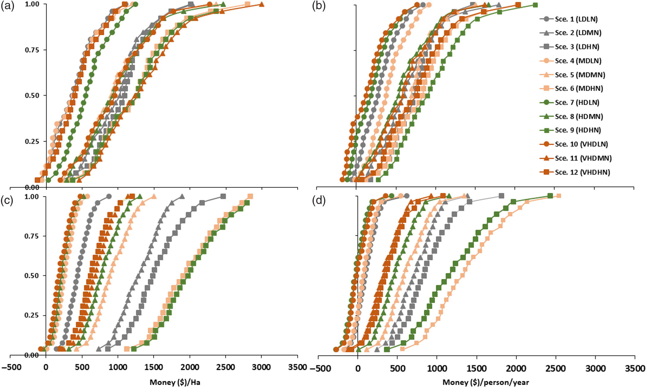
The returns to land and labor measured in US$ per ha per adult male equivalent of family labor are presented in Figure 7 for SAMMAZ 41 (A and B) in the SS and SAMMAZ 15 (C and D) in the NGS. The cumulative distribution function (CDF) plot for SAMMAZ 41 shows that all the LD scenarios will return less than US$500 ha−1 except for scenario 1 (LDLN) where a return of US$600 ha−1 is possible at 50% probability level of non-exceedance. For the same low-intensity scenarios, the probability of getting a return to land above US$1000 ha−1 was only 10% (i.e. only 2.6 out of the 26 years simulated). Increasing sowing density from 2.6 to 5.3 plants m−2 had a 75% probability of producing an increased return to land for at least 40% of N applied. For the low and medium N application scenarios, increased returns to land of 44 and 46% were recorded, while an increase of just 47% was recorded for the high N scenario. For the high (6.6 plants m−2) and very high (8.8 plants m−2) densities scenarios, however, a 75% probability of exceeding a return of over US$1000 ha−1 was possible when the recommended N fertilizers were applied. The lowest returns to land were recorded for the very high-density (VHD) scenarios under low N fertilization.
Cumulative distribution function plot for monetary return per hectare and unit of family labor (A and B = for Sammaz 41) and (C and D = Sammaz 15) for different sowing densities and nitrogen rates.

For the monetary return to labor, however, all the LD scenarios had only a 25% probability of returning less than US$500 per person per season and none of the low-density scenarios returned up to US$1000 per person. The HDHN scenario had the biggest probability of producing higher returns to labor (US$500 to US$700 at 75% probability, above US$1000 at 50% probability, and up to US$2000 with a 5% probability). Negative returns to labor were reported for 4 out of the 26 years for the VHD and low N (VHDLN) scenarios and 2 years for the high-density and low N (HDLN) scenarios. The possibility of negative returns to land was simulated in 3 years for the VHD and high N (VHDHN) applications scenario and only 1 year for the HDHN application scenario. For SAMMAZ 41 in the SS, mean monetary return per ha increased with increasing sowing density for all the low N application scenarios up to the highest sowing density tested. The lowest mean return to land was recorded for scenario 1 (2.6 plants m−2 + 30 kg N ha−1) while the highest was recorded for scenario 10 (8.8 plants m−2 + 30 kg N ha) indicating that elevating sowing density could increase income even at low N application rates. The highest mean return to land (US$1336.1) was recorded for scenario 9 (8.8 plants m−2 + 90 kg N ha−1). For the mean return to labor, however, the lowest amount (US$150.6) was recorded for scenario 10 (8.8 plants m−2 + 90 kg N ha−1). The highest mean return to labor (US$957.7) was also recorded for scenario 9.
In the NGS, higher returns to both land and labor were recorded than in the SS. The mean monetary returns to land were higher at high N applications for the low, medium, and high sowing densities. For the VHD scenario, however, monetary returns per hectare were low even when the highest level of N was applied. All the LD scenarios (scenarios 1, 4, 7, and 10) had only 25% chance of returning at least US$500 per unit hectare, although it is only in 1 of the 26 years simulated (3.8% chance) that a low sowing density could return up to US$1000 per hectare. All the LD scenarios have less than 50% chance of producing above US$500 per hectare and per male adult equivalent person. The scenario with the highest mean monetary return per hectare was scenario 9 (HDHN) although the difference with scenario 6 (medium-density + high N) was only 3.3%. Scenario 6 recorded the highest returns per person followed by scenario 9. Mean negative returns were recorded for scenarios 10 (8.8 plants m−2 + 30 kg N ha−1) and 7 (6.6 plants m−2 + 30 kg N ha−1).
Discussion
Model calibration and evaluation
The model calibrations resulted in the accurate predictions of the field measured phenology and yield parameters with high a degree of confidence as indicated by the model statistics. This close agreement between predicted and observed yield and phenology variables for both calibration and evaluation experiments is an indication that the model can be used to predict the performance of the maize genotypes across different locations and under variable management conditions in the Nigerian Savannas. Phenology (flowering and maturity) is controlled by the coefficients P1 and P5 in CERES-Maize model. The present calibration showed accurate predictions of phenology which is the most important step in the model calibration exercise (Archontoulis et al., Reference Archontoulis, Miguez and Moore2014). According to Robertson et al. (Reference Robertson, Carberry, Huth, Turpin, Probert, Poulton, Bell, Wright, Yeates and Brinsmead2002), accurate calibration of phenology enables models to capture all genotypic variations that affect the leaf area development, biomass production, and grain yield. Very good agreements were observed between observed and simulated grain yields in both calibration and evaluation experiments. This can be attributed to accurate measurements of the coefficients, G2 (sink size) and G3 (sink strength). The accurate capture of seasonal and locational variations is as a result of adjustments made to the coefficients RUE and SLPF. According to Pantazi et al. (Reference Pantazi, Moshou, Alexandridis, Whetton and Mouazen2016), an accurate prediction of yield in crop modeling is the most important step when the overall objective of the modeling exercise is the improvement of crop management. The closeness of fit between observed and predicted parameters in the calibration and evaluation steps is an indication that the model is robust and accurate enough to make wider applications across the environments under study. The results are also in line with previous findings from the same agro-ecologies (Jagtap et al. Reference Jagtap, Alabi and Adeleye1998, Reference Jagtap, Abamu and Kling1999; Jibrin et al. Reference Jibrin, Kamara and Ekeleme2012; Gungula et al. Reference Gungula, Kling and Togun2003).
Sensitivity and scenario analyses
The result of the sensitivity analyses follows expected trends of published data on sowing density with the extra-early and early varieties showing greater response to sowing density increases than the late and intermediate varieties (Edwards et al., Reference Edwards, Purcell and Vories2005; Sangoi et al., Reference Sangoi, Gracietti, Rampazzo and Bianchetti2002; Tollenaar and Lee, Reference Tollenaar and Lee2002). The extra-early variety produced the highest grain yields with sowing density of 10 plants m−2, the early varieties produced the highest grain yields at sowing density of eight plants m−2, while the late and intermediate varieties produced the highest grain yields at sowing density of six plants m−2. Previous reports by Edwards et al. (Reference Edwards, Purcell and Vories2005) show that higher planting densities are required for early maturing varieties than full-season varieties. This is because early varieties usually have smaller leaves, which means more plants are needed per area to reach the same amount of cumulative intercepted radiation (Tollenaar et al., Reference Tollenaar, Deen, Echarte and Liu2006). The particularly low simulated yield for the late-maturing varieties for sowing densities above six plants m−2 could be due to the shading ability and the long grain filling duration of such varieties (Van Roekel and Coulter, Reference Van Roekel and Coulter2011). The fact that the model was able to capture these expected variations is an indication of the robustness of the calibration and evaluation steps.
It is important to understand what best combinations of agronomic practices will optimize yields for smallholder maize growers. Crop models can be used to simulate such practices if properly calibrated and validated. Here, the CERES-Maize model was used to create two different scenarios with various combinations of sowing density and N fertilizer rates. Results of the scenario analyses show that with low N fertilization (30 kg N ha−1), increasing planting density did not increase grain yields. For the extra-early and late varieties, yields stagnated when planting densities were increased with low N applications, while for intermediate and late varieties a linear decline in yield was observed with every increase in planting density at low N application. Similar trends were observed with the application of 60 kg N ha−1 for the late and intermediate varieties, but slight gains in yield were observed for the early varieties where increasing density from 2.6 to 5.3 and 6.6 plants m−2 produced yield increases of 8.8 and 12.3% respectively. This suggests that for early varieties, higher densities could lead to increased grain yields even when low N rates are applied. For high N applications (90 in SS and 120 in NGS), yield gains were observed for every successive increase in planting density up to 8.8 plants m−2 for extra-early and early varieties and 6.6 plants m−2 for intermediate and late varieties. This finding confirms previous claims by Jagtap et al. (Reference Jagtap, Abamu and Kling1999) that increased responses to the sowing density are possible for small, compact varieties with erect leaves in Nigeria. Interestingly, the findings also show that there is a possibility for yield increase when maize is planted above the recommended sowing densities without increasing the recommended fertilizer rates. In fact, for the early varieties, the simulations show that high grain yields are possible with increasing sowing densities even if N applications were 30 kg lower than the current recommendations.
Economic analyses
For smallholder farmers, the economic return and risk associated with the adoption of new technology go beyond mere yield variability. Clearly, any new technology that could increase income per unit of land and/or per laborer is an economic rational opportunity for those farmers. The results of the economic analyses using simulated yields and historical input and output prices show that increasing sowing density leads to economic gains in both agro-ecologies if the sowing-density increases are accompanied by increased N application rates. Traditionally, farmers in the study location choose both sowing densities and N fertilizer rates below the recommendation from extension programs, believing that an additional number of plants per area necessarily implies additional N fertilizer that they cannot or hardly afford. Findings confirm that the sowing density of maize can be increased while maintaining the current N fertilizer recommendations.
The dramatic increase in monetary return per hectare is due to the extra yield from the highest planting density even at low N application. This finding is a clear indication that even under low N application in smallholder farms, sowing density of the extra-early and early varieties could be increased to produce higher yields and higher incomes per hectare. This finding confirms previous claims by (Edwards et al., Reference Edwards, Purcell and Vories2005) that yields of short-season maize varieties are usually maximized at higher planting densities. They stated that increasing the plant population of early varieties will compensate for the reduced grain-fill durations, increase light interception over the entire season, and result in a similar yield potential as full-season varieties.
Mean returns to land and family labor decreased continuously when sowing density was increased in the low N scenarios for SAMMAZ 15 in the NGS. Applying 30 kg N ha−1 and planting 2.6 plants m−2 produced a mean return of US$457.6 ha−1, but when sowing density was increased to 5.3, 6.6, and 8.8 plants m−2, declines in the income of 40.9, 50.1, and 55.9% respectively were recorded. This means that increasing sowing density at low N leads to a huge reduction of economic returns per hectare. The highest returns to land were recorded for the high density + high N (6.6 plants m−2 + 120 kg N ha−1) scenarios, while the highest returns to labor were recorded for the medium density + high N (5.3 plants m−2 + 120 kg N ha−1) scenarios. This result indicates that for the intermediate varieties, VHDs (above 6.6 plants m−2) will lead to reduced income. Very low densities become even less economically optimal at high N application because the yield increase is negligible and does not cover the additional expense of fertilizers and the labor requirements.
Conclusion
In the current study, the CERES-Maize model produced long-term simulations for grain yield and monetary returns per unit of land and unit of labor. Findings from the simulation studies indicate that contrary to most assertions, the sowing density of all the current varietal groups of maize in Nigeria could be increased without applying N fertilizers above the recommended rates in Sudan and Northern Guinea Savannas. For the early and extra-early varieties, the highest grain yields were simulated for sowing density of 8.8 plants m−2 and N rate of 90 kg N ha−1 while for the intermediate and late varieties the highest grain yields were simulated for sowing density of 6.6 plants m−2 and N rate of 120 kg N ha−1. In SS, the extra-early and early varieties could provide more income per unit of land under the intensive systems (8.8 plants m−2 and 90 kg N ha−1), but the largest monetary return to labor can be achieved under the semi-intensive agronomic practice (6.6 plants m−2 and 90 kg N ha−1). In NGS, return to land is maximized under semi-intensive agronomic practices (6.6 plants m−2 and 120 kg N ha−1) and return to labor is maximized when the recommended sowing density of 5.3 plants m−2 is combined with high N (120 kg ha−1) applications.