1. Introduction
One of the central problems of macroeconomic theory is understanding the impact of real shocks on aggregate variables like output and unemployment. Real shocks vary in their granularity from idiosyncratic firm-level productivity shocks to large-scale events like wars, natural disasters, and the COVID lockdowns. Most macroeconomic models used to study the impact of real shocks assume that the economic system perennially remains at equilibrium. This is a problematic assumption when it comes to shocks that prod the economy away from equilibrium. The COVID lockdown is one such shock. The lockdown is in essence a binding quantity constraint with heterogeneous impact across different sectors of the economy. This means that the lockdown would have triggered disequilibrium dynamics particularly as the shock propagated through the buyer–seller relations between firms across different sectors. In this paper, we develop a model capable of exhibiting disequilibrium dynamics to estimate the impact of the COVID lockdown. Notably, our model places special emphasis on the unemployment dynamics that emerge from the propagation of a shock through a network economy.
Our model is built on Gualdi and Mandel’s (Reference Gualdi and Mandel>2016) out-of-equilibrium extension of Acemoglu et al.’s (Reference Acemoglu, Carvalho, Ozdaglar and Tahbaz-Salehi>2012) model of a network economy. Firms are related to each other through a production network. Each firm buys inputs from a subset of firms and sells output to another subset of firms. Each firm produces using a CES production function nested in a Cobb–Douglas function. Intermediate inputs are combined using the CES part, and therefore each firm’s input combination depends on input prices. A representative household buys goods using a Cobb–Douglas utility function and supplies a fixed quantity of labor. Prices are determined by direct agent interactions rather than a tatonnement process. We unbundle the decisions that are assumed to occur simultaneously in standard general equilibrium models. More specifically, pricing and production decisions are not contemporaneous within our model. Firms purchase inputs using cash balances to produce the output that is sold at the next time step. The revenues earned by selling output become cash balances for the purchase of inputs. Firms therefore may be thought of as facing cash-in-advance constraints. Each time step, firms determine prices based on the stock of output carried from the last time step and the nominal demand received this time step. When prices are sticky, each firm charges a price which is a linear combination of last period’s price and current period’s local market clearing price. Price stickiness generates inventory dynamics as firms carry unsold output to the next time step.
Within such a multi-market setting, real shocks generate disequilibrium dynamics. The system goes out of equilibrium because the flows of intermediate inputs are not the equilibrium flows consistent with the primitives that define the economy. Disequilibrium spills over from one market to another disturbing partial equilibrium in all parts of the economy. Such disequilibrium dynamics are capable of generating unemployment. More specifically, within our setting, firms expand and contract in response to changes in the flows of inputs amidst the disequilibrium dynamics generated by a shock. If the labor released by contracting firms is not frictionlessly absorbed by expanding firms, the propagation of a shock will generate disequilibrium unemployment. These dynamics are of theoretical and practical interest. From a theoretical point of view, they are a new source of frictional unemployment. From a practical point of view, such disequilibrium unemployment may aggravate the impact of the shock. We formalize the friction in the movement of labor from one firm to another using a “job-finding rate,” which is the rate at which unemployed labor finds new jobs. Within our model, the job-separation rate is endogenously determined as it depends on the fluctuations in firms’ sizes in the transition from one equilibrium to another. The job-separation rate rises after a real shock because some firms contract their production levels as the shock propagates through the production network. The rise in the job-separation rate, coupled with the exogenously fixed job-finding rate, generates unemployment in the transition from one equilibrium to another. The root cause of disequilibrium unemployment within our network economy is the fluctuations in firm sizes, which themselves arise from the sensitivity of production decisions to current market conditions.
We use the afore-described disequilibrium network economy model to study the impact of the COVID lockdown. Note that the COVID lockdowns are not productivity shocks. In other words, it is not that firms became less efficient at combining inputs. Rather the lockdowns are temporary quantity constraints with heterogeneous limits on different sectors. We estimate the direct impact of the lockdown using Federal Reserve and Census Bureau data on sectoral economic activity for March 2020. We then measure the amplification of the direct shocks by the production network using computational experiments on the US economy calibrated to granular data on buyer–seller relations between firms.
1.1. Related literature
Our paper is related to a growing literature on the macroeconomic impact of the pandemic.Footnote 1 A number of contributions to the literature represent the lockdowns as some kind of productivity shock [Baqaee and Farhi (Reference Baqaee and Farhi>2019) and Fornaro and Wolf (Reference Fornaro and Wolf>2020)]. In this paper, we aim at a more accurate microeconomic representation of the lockdowns in the form of quantity constraints. To do so, we build on a model which we have used in the past to analyze out-of-equilibrium dynamics in numerous settings, including the dynamics of economic growth [Gualdi and Mandel (Reference Gualdi and Mandel>2016, Reference Gualdi and Mandel>2018)] and the dynamics of prices [Mandel et al. (Reference Mandel, Taghawi-Nejad and Veetil>2019) and Mandel and Veetil (Reference Mandel and Veetil>2021)]. In Mandel and Veetil (Reference Mandel and Veetil>2020), we used a variant of the model calibrated to sectoral input–output data to study the impact of the COVID lockdowns. This paper differs from Mandel and Veetil (Reference Mandel and Veetil>2020) in several ways. The first of which is that the version of the model presented in this paper incorporates unemployment. No one has so far studied the interaction between network dynamics and unemployment, particularly in the context of such a large shock to the economy. The second difference is that in our previous work, we calibrated the model to input–output data, while in this paper we present significantly more granular calibration with firm-level data. In some senses, we illustrate the possibility of ultimately calibrating such models to granular data on the complete economy and then using these models as testbeds for experiments before the implementation of policy. The third difference is that in this paper we analyze the intricate relation between price stickiness and the cost of disturbance to a network economy. Notably, price stickiness interacts with the network setting to generate some counterintuitive results with regard to the cost imposed by the propagation of an exogenous shock.
Certain aspects of our approach to understanding the dynamics of a network economy is closely related to that of Pichler and Farmer (Reference Pichler and Farmer>2021) and Pichler et al. (Reference Pichler, Pangallo, del Rio-Chanona, Lafond and Farmer>2022). They emphasize the complexity of the relation between final demand and GDP within a network setting. Curiously enough, within a network setting, a decrease in the final demand relative to intermediate demand can be “beneficial” for the economy as whole in so far as the resources allocated to intermediate use generate final goods in the future. Therefore, the specifics of the allocation and reallocation of goods between intermediate and final use is the primary driver of the aggregate dynamics of a network economy. In fact, such a reallocation of resources is what generates the temporary decline in GDP after the relaxation of the lockdown within our model.
1.2. Organization of the paper
The rest of our paper is organized as follows. Section 2 presents the model. Section 3 calibrates the model to the US production network. Section 3 also estimates firm-wise lockdown shock using data from the Federal Reserve and the Census Bureau. Section 4 presents results from computational experiments in which we implement empirically grounded lockdown shocks on the model calibrated to the US production network. Section 5 discusses the relation between price stickiness and the cost of the lockdown. Section 6 presents concluding thoughts. The Supplementary Appendix contains results from additional experiments and justification for certain model assumptions. Notably, Section 1 of the Supplementary Appendix discusses the problem of accounting for GDP within a network economy particularly when the system is capable of exhibiting disequilibrium dynamics. The model code is available at bitbucket.org/VipinVeetil/networkeconomy.
2. Baseline model
2.1. General equilibrium characteristics
There is a finite set of monopolistically competitive firms and a representative household. We denote the set of firms (which is also the set of goods) by
 $N=\{1,\cdots,n\}$
and the representative household by the index
 $0$
. The representative household supplies a constant quantity of labor
 $l$
(normalized to
 $1$
) and has preferences represented by a Cobb–Douglas utility function of the form:
 \begin{equation} u\!\left(x_{1},\cdots,x_{n}\right)={\prod }_{i=1}^{n}{x}_{i}^{\beta _{i}} \end{equation}
with
 ${\sum }_{i=1}^{n}\beta _{i}=1$
and
 $\beta _{i}\gt 0$
for all
 $i\in N$
.
The firms interact through a production network. This network is characterized by an adjacency matrix
 $M=(m_{ij})_{i,j\in M}$
such that
 $m_{ij}=1$
if
 $j$
is a supplier of
 $i$
and
 $m_{ij}=0$
otherwise.
 $S_{i}(M)\;:\!=\;\{j\in N| m_{ij}=1\}$
denotes the set of suppliers of firm
 $i$
and
 $n_{i}(M)$
its number of suppliers. Each firm
 $i$
uses a Cobb–Douglas production function across labor and intermediate inputs, with a CES aggregator across intermediate inputs. More specifically, each firm
 $i$
’s production function
 $f_{i}\colon {\mathrm{\mathbb{R}}}_{+}^{M}\rightarrow \mathrm{\mathbb{R}}_{+}$
is of the following form:
 \begin{equation} f_{i}\!\left(l_{i},\left(y_{ij}\right)_{j=1,\ldots,{n_{i}}}\right)=k_{i}\!\left(M\right){l}_{i}^{\alpha }\!\left(\sum _{j\in S_{i}(M)}{y}_{ij}^{\sigma }\right)^{\frac{1-\alpha }{\sigma }} \end{equation}
where
 $l_{i}\in \mathrm{\mathbb{R}}_{+}$
is the labor input,
 $y_{ij}\in \mathrm{\mathbb{R}}_{+}$
is the input of good
 $j, \text{and}\, \alpha$
is the Cobb–Douglas exponent.
 $k_{i}(M)$
is a scaling parameter which guarantees that a firm’s productivity does not increase with the number of input sellers:
 \begin{equation} k_{i}\!\left(M\right)=\frac{(1-\sigma )}{\sigma }n_{i}\!\left(M\right)^{\frac{(1-\sigma )}{\sigma }} \end{equation}
Remark 1
(The share of labor and disequilibrium dynamics). The parameter
 $\alpha$
is the share of labor in equilibrium, but it needs not be the share of labor out of equilibrium. More specifically,
 $\alpha$
is the share of labor in nominal income. When the economy is out of equilibrium, the dynamics of relative prices along with nominal income will determine the share of labor in real income. Therefore, when out of equilibrium, the real share of labor will tend to be different from
 $\alpha$
.
The network structure
 $M$
and the elasticity of substitution
 $\sigma$
define a general equilibrium economy
 $\mathrm{\mathcal{E}}(\sigma,M).$
In particular, the limit case corresponding to Cobb–Douglas production functions obtained when
 $\sigma \rightarrow 0$
is denoted by
 $\mathrm{\mathcal{E}}(0,M).$
The standard definition of equilibrium for the class of economies
 $\mathrm{\mathcal{E}}(\sigma,M)$
is as follows.
Definition 1.
A general equilibrium of the economy
 $\mathrm{\mathcal{E}}(\sigma,M)$
is a collection of prices
 $(\overline{p}_{1},\ldots,\overline{p}_{n})\in {\mathrm{\mathbb{R}}}_{+}^{N}$
, wage
 $\overline{p}_{0}\in \mathrm{\mathbb{R}}_{+}$
, production levels
 $(\overline{q}_{1},\ldots,\overline{q}_{n})\in {\mathrm{\mathbb{R}}}_{+}^{N}$
, consumption levels
 $(\overline{x}_{1},\ldots,\overline{x}_{n})\in {\mathrm{\mathbb{R}}}_{+}^{N}$
, labor
 $\{\overline{l}_{i}\}_{i\in N}\in {\mathrm{\mathbb{R}}}_{+}^{N}$
, and commodity flows
 $\{\overline{y}_{ij}\}_{i,j\in N}\in {\mathrm{\mathbb{R}}}_{+}^{N\times N}$
such that:
-
1. Markets clear:
(4) \begin{equation} \forall i\in N,\,\overline{q}_{i}=\overline{x}_{i}+{\sum }_{j=1}^{n}\overline{y}_{ji},\forall i\in N\quad \left(\text{goods} \, \text{market}\right) \end{equation}
(5)
\begin{equation} 1={\sum }_{i=1}^{n}\overline{l}_{i}\quad \left(\text{labor} \, \text{market}\right) \end{equation}
-
2. The representative consumer maximizes utility, that is
$(\overline{x}_{i})_{i\in N}$
is a solution to:(6)
\begin{align} \begin{cases} \max & u(x_{1},\cdots,x_{n})\\[5pt] s.t. & {\sum }_{i=1}^{n}\overline{p}_{i}x_{i}\leq \overline{p}_{0} \end{cases} \end{align}
-
3. Firms maximize profits, that is for all
$i\in N,$
$(\overline{q}_{i},\overline{l}_{i},(\overline{y}_{ij})\in {\mathrm{\mathbb{R}}}_{+}^{N+2}$
is a solution to:(7)
\begin{align} \begin{cases} \max & \overline{p}_{i}q_{i}-\overline{p}_{0}l_{i}-\sum _{j\in N}\overline{p}_{j}y_{ij}\\[5pt] s.t & q_{i}\leq f_{i}(l_{i},(y_{ij})_{j\in N}) \end{cases} \end{align}


It is straightforward to check that the equilibrium of the economy
 $\mathrm{\mathcal{E}}(M)$
is unique (noting in particular that the representative agent has a strictly concave utility function). From a network perspective, the general equilibrium of the economy as well as out-of-equilibrium dynamics induce flows of good across the network
 $M$
. Given production functions with constant returns to scale, these flows can be characterized by a weighted network which extends
 $M$
by specifying the share of spending firm
 $i$
directs to firm
 $j$
. Namely, one has the following definition:
Definition 2.
Given a price vector
 $p\in {\mathrm{\mathbb{R}}}_{+}^{N},$
the network of input shares
 $A_{M}(p)=(a_{ij}(p))_{i,j\in N}$
is defined by solving for each
 $i\in N$
:
 \begin{equation} \begin{array}{cccc} & \max _{a_{i\cdot }\in \mathrm{\mathbb{R}}^{{S_{i}}(M)}} & & f_{i}\!\left(\frac{\alpha }{w},\left(\frac{a_{i1}}{p_{1}},\cdots,\frac{a_{i{n_{i}}(M)}}{p_{{n_{i}}(M)}}\right)\right)\\[5pt] & \mathrm{s}.\mathrm{t}. & & \sum a_{ij}+\alpha =1 \end{array} \end{equation}
which yields the solution:
 \begin{equation} \begin{array}{c} a_{ij}\!\left(p\right)=\frac{1-\alpha }{1+{\sum }_{j\in S_{i}(M)}^{n}\left(\frac{p_{i}}{p_{j}}\right)^{\sigma /(1-\sigma )}} \end{array} \end{equation}
In words,
 $a_{ij}(p)$
represents the share of nominal expenses of firm
 $i$
directed towards firm
 $j$
given a price vector
 $p.$
Footnote
2
Remark 2.
In the limit case of a Cobb–Douglas economy, the network of input shares is independent of the price vector and simply denoted by
 $A_{M}$
to emphasize the dependence on the underlying network structure
 $M.$
2.2. Out-of-equilibrium dynamics
Following Gualdi and Mandel (Reference Gualdi and Mandel>2016), we introduce decentralized out-of-equilibrium dynamics in this framework. Time is discrete and indexed by
 $t\in \mathrm{\mathbb{N}}.$
Each firm
 $i\in N$
is characterized at every time step
 $t\in \mathrm{\mathbb{N}}$
by its price
 ${p}_{i}^{t}\in \mathrm{\mathbb{R}}_{+},$
its stock of output
 ${q}_{i}^{t},$
its working capital
 ${w}_{i}^{t}\in \mathrm{\mathbb{R}}_{+}$
, and the allocation of its expenditures
 ${a}_{i\cdot }^{t}\in \mathrm{\mathbb{R}}^{{\overline{S}_{i}}(M)}.$
Where by “working capital” we mean the liquidity available to firms to purchase inputs. Put differently, firms in the model can be thought of as facing a cash-in-advance constraint. The household is characterized by its wage
 ${p}_{0}^{t}$
and its labor supply
 $l^{t}=1.$
Each agent engages in a sequence of local interactions every period with its buyers and sellers. More specifically, the following sequence of events take place at every time step
 $t\in \mathrm{\mathbb{N}}$
:
-
1. Agents determine nominal demand to their suppliers according to network weights: the nominal demand of firm
$i$
towards firm
$j$
is
$a_{ij}{w}_{i}^{t}$
. The nominal demand of the household towards firm
$j$
is given by
$\beta _{j}{w}_{0}^{t}.$
And the nominal demand of firm
$i$
for labor is
$\alpha {w}_{i}^{t}.$
-
2. Each firm
$i$
adjusts its prices towards the market clearing value using the following equation:


 \begin{equation} {p}_{i}^{t}=\rho {p}_{i}^{t-1}+(1-\rho ){p}_{i}^{*t} \end{equation}
where
 $\rho \in [0,1]$
is a parameter measuring the speed of price adjustment and
 ${p}_{i}^{*t}$
is the local market clearing price of firm
 $i$
. Given the nominal demand
 $\sum _{j\in N}a_{ji}{w}_{j}^{t}+\beta _{i}{w}_{0}^{t}$
and the output stock
 ${q}_{i}^{t},$
 ${p}_{i}^{*t}$
is given by the following equation:
 \begin{equation} {p}_{i}^{*t}=\frac{\sum _{j\in N}a_{ji}{w}_{j}^{t}+\beta _{i}{w}_{0}^{t}}{{q}_{i}^{t}} \end{equation}
(Note that the local market clearing price
 ${p}_{i}^{*t}$
is not necessarily the general equilibrium price
 $\overline{p}_{i}$
, because output and nominal demand are not exogenously pinned to their equilibrium values.)
-
3. The wage is set to:
 \begin{equation} {p}_{0}^{t}=\frac{\sum _{i\in N}\alpha {w}_{i}^{t}}{l^{t}} \end{equation}
-
4. Goods are allocated as follows.
-
If the price of a good
${p}_{j}^{t}$
is greater than or equal to the local market clearing price
${p}_{j}^{*t}$
then for all
$i,j\in N\colon$


 \begin{equation} {y}_{ij}^{t}=\frac{a_{ij}{w}_{i}^{t}}{{p}_{j}^{t}}\quad \left(\text{inputs} \, \text{allocation}\right) \end{equation}
 \begin{equation} {x}_{i}^{t}=\frac{\beta _{i}{w}_{0}^{t}}{{p}_{i}^{t}}\quad \left(\text{consumption} \, \text{allocation}\right) \end{equation}
-
Otherwise, if the price of a good
${p}_{j}^{t}$
is less than the market clearing price
${p}_{j}^{*t},$
agents are rationed proportionally to their demand and one has for all
$i,j\in N\colon$


 \begin{equation} {y}_{ij}^{t}={r}_{i}^{t}a_{ij}{w}_{i}^{t}\quad (\text{inputs} \, \text{allocation}) \end{equation}
 \begin{equation} {x}_{i}^{t}={r}_{0}^{t}\beta _{i}{w}_{0}^{t}\quad (\text{consumption} \, \text{allocation}) \end{equation}
where
 ${r}_{i}^{t}=\frac{a_{ji}{w}_{j}^{t}}{\sum _{j\in N}a_{ji}{w}_{j}^{t}+\beta _{i}{w}_{0}^{t}}$
and
 ${r}_{0}^{t}=\frac{\beta _{i}{w}_{0}^{t}}{\sum _{j\in N}a_{ji}{w}_{j}^{t}+\beta _{i}{w}_{0}^{t}}$
.
-
5. Labor is allocated among firms as follows:
 \begin{equation} {l}_{i}^{t}=\frac{{w}_{i}^{t}l^{t}}{\sum _{j\in N}{w}_{j}^{t}}\quad \left(\text{labor} \, \text{allocation}\right) \end{equation}
-
6. Firms compute the optimal shares of expenditure on intermediate inputs:
 \begin{equation} {a}_{ij}^{t+1}\;:\!=\;a_{ij}\!\left(p^{t}\right)=\frac{1-\alpha }{1+{\sum }_{j=1,i\neq j}^{n}\left(\frac{{p}_{i}^{t}}{{p}_{j}^{t}}\right)^{\sigma /(1-\sigma )}} \end{equation}
-
7. The working capital of each firm is updated on the basis of revenue, for all
$i\in N$
:

 \begin{equation} {w}_{i}^{t+1}=\sum _{j\in N}{a}_{ji}^{t}{w}_{j}^{t} \end{equation}
And the household’s wealth
 ${w}_{0}^{t+1}$
is simply
 ${p}_{0}^{t}l^{t}$
.
-
8. Firms produce and update their inventory of output for the next period. Namely, for all
$i\in N\colon$

 \begin{equation} {q}_{i}^{t+1}=f_{i}\!\left({l}_{i}^{t},{y}_{i\cdot }^{t}\right)+\left({q}_{i}^{t}-\sum _{j\in N}\left({y}_{ji}^{t}-{x}_{i}^{t}\right)\right) \end{equation}
The dynamical system defined by equations (10) to (20) was introduced in Gualdi and Mandel (Reference Gualdi and Mandel>2016), to formally analyze out-of-equilibrium dynamics. Yet, a major shortcoming of that model in view of empirical applications like the COVID lockdowns is the absence of unemployment. In that model, the wage rate was assumed to be fully flexible. In order to relax this counterfactual assumption, we consider a version of the model in which wage rigidity generates imbalances in the labor market.
Remark 3 (Upward and downward wage rigidity). We assume that wages are rigid upwards and downwards. There is considerable empirical evidence to support the hypothesis of downward rigidity of wages and some supporting upward rigidity. From a theoretical point of view, in the presence of transient dynamics, downward rigidity of wages will tend to generate some upward rigidity. More specifically, given that the economy is going through a transition, firms are unlikely to set wages which are fully flexible upwards, knowing well that once set it will be difficult to decrease the wage in the future when temporary circumstances change.
Let us denote the nominal demand for labor of firm
 $i$
at time step
 $t$
by
 ${d}_{i}^{t}\;:\!=\;\alpha {w}_{i}^{t}$
and the total demand for labor by
 $\sum _{i\in N}{d}_{i}^{t}$
. Suppose
 $\sum _{i\in N}{d}_{i}^{t}\lt \sum _{i\in N}{d}_{i}^{t-1}.$
If prices ought to remain downward rigid, in view of equation (11), labor supply must adjust downwards proportionally to
 $\frac{\sum _{i\in N}{d}_{i}^{t}}{\sum _{i\in N}{d}_{i}^{t-1}}.$
In other words, a share
 $s^{t}\;:\!=\;\left(1-\frac{\sum _{i\in N}{d}_{i}^{t}}{\sum _{i\in N}{d}_{i}^{t-1}}\right)$
of labor must become unemployed. We further assume that there are search and matching frictions in the labor market. These frictions are represented by parameter
 $\phi \in (0,1)$
which denotes the rate at which the unemployed are resorbed into employment. This means that the unemployment rate
 $u^{t}$
is given by the following equation:
 \begin{equation} u^{t}=(1-\phi )(u^{t-1}+s^{t}(1-u^{t-1})) \end{equation}
(Note that
 $s^{t}(1-u^{t-1})$
is multiplied by
 $1-\phi$
because those who are unemployed at time
 $t$
get a chance to look for a job at the same time step.) The quantity of labor available for production at each time step is
 \begin{equation} l^{t}=1-u^{t} \end{equation}
We refer to a steady state of the dynamics defined by equations (10) to (22) as steady state of the economy
 $\mathrm{\mathcal{E}}(M,\sigma ).$
At such a steady state, equations (10) and (11) imply market clearing, equation (18) implies the minimization of cost (and thus the maximization of profits as there are constant returns to scale), equation (14) implies utility maximization, and equation (21) together with the fact that one must have
 $s^{t}=1$
at steady state implies there is no unemployment. Overall:
Proposition 1.
The steady state of the economy coincides with the general equilibrium of the economy
 $\mathrm{\mathcal{E}}(M,\sigma ).$
When
 $\phi =1,$
the dynamics coincide with those considered in Gualdi and Mandel (Reference Gualdi and Mandel>2016) and Mandel et al. (Reference Mandel, Taghawi-Nejad and Veetil>2019).Footnote
3
In the long run, these dynamics convergence to general equilibrium independently of
 $\phi$
and
 $\sigma$
. In the short run, these dynamics induce a propagation of disequilibrium shocks upstream through changes in demands and downstream through changes in prices. The impact of the network structure on the dynamics can be highlighted by writing the dynamics of working capital in matrix form:
 \begin{equation} w^{T}\;:\!=\;\left({\prod }_{t=1}^{T-1}A_{M}\!\left(p^{t}\right)\right)\!w^{0} \end{equation}
3. Setting up the model for the lockdown experiments
We calibrate the model to the US economy using data on 207,995 buyer–seller relations between 70,077 firms. Put differently, the adjacency matrix of the model is taken from real-world data on production relations. The data set comes from Standard and Poor’s Capital IQ. It contains buyer–seller relations formed between the years
 $2005$
and
 $2017$
without information on the exact year at which the link was formed. The Capital IQ data set contains an order of magnitude more firms and linkages than data on relations between publicly traded firms reported by Atalay et al. (Reference Atalay, Hortacsu, Roberts and Syverson>2011) and three orders of magnitude more entities than the Input–Output Table. Section 3 of the Supplementary Appendix contains information on the sectoral distribution of firms in our data set as compared to that in the US economy.
We also calibrate our model to the empirically observed distribution of household expenditure across different sectors of the economy. More specifically, we use data on the sectoral distribution of the Personal Consumption Expenditure from the Input-Output Table of the USA to determine the share of household expenditure on different firms within our data set. We match household expenditures on different sectors at two digit NAICS level by dividing the expenditure among firms within each group in our data set. Lastly, we compute the sectoral composition of the lockdown shock using productivity data from the Federal Reserve and sales data from the Census Bureau. We then use these sectoral estimates to compute the size of the lockdown shock for different firms within our data set.
3.1. The lockdown shock data
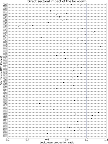
According to publicly available information presented in the entry on “national responses to the 2019–20 coronavirus pandemic” on Wikipedia, parts of the US economy entered a 50-day lockdown on 19 and 20 of March 2020. The lockdown did not apply equally to all sectors of the economy. We model the lockdown shock using data on sectoral output released by the Federal Reserve and Census Bureau. More specifically, we derive the impact of the lockdown across several sectors using data on the sectoral distribution of industrial production for March 2020 released by the Federal Reserve on 15 April 2020. The Fed data contains information on the level of production in the following sectors: NAICS 11 [Agriculture, Forestry, Fishing, and Hunting], NAICS 21 [Mining, NAICS 22 Utilities], NAICS 31-33 [Manufacturing], NAICS 51 [Finance and Insurance], and NAICS 56 [Administrative and Support Services]. Figure 1 presents the ratio of output during the lockdown period in March to the output during “normal” times. The figure contains data on 89 sectors at the four-digit NAICS level. The normal level of output is computed as the mean output (adjusted for seasonal variation) of December 2019, January 2020, and February 2020. We assume output was normal in March till the lockdown began on 20 March 2020 and, therefore, ascribe the full change of output in March relative to the normal to the last 10 days of the month. Figure 1 shows that there is sizeable heterogeneity in the impact of the lockdown across different sectors of the economy.Footnote 4
The Fed data does not contain information on all sectors of the economy. We therefore combine the Fed data with the Census Bureau’s advanced estimates of sales of retail and related sectors for March 2020 released on 15 April 2020. The Census data set contains information on NAICS 44-45 [Retail Trade]. Combining the Fed data with the Census data does not however exhaust all sectors of the US economy. These data sets do not contain information on NAICS 61-62, 71-72, 81, and 92. We assume the ratio of lockdown to normal production in these sectors is as follows: NAICS 61 [Education]: 1, NAICS 62 [Health Services]: 1, NAICS 71 [Arts, Entertainment and Recreation]: 0.5, NAICS 72 [Accommodation and Food Services]: 0.5, NAICS 81 [Other Services]: 1, and NAICS 92 [Public Administration]: 1. These estimates draw on scenarios considered by IFO-Institute (>2020) to study the impact of the lockdown in Europe. We have been conservative in assuming NAICS sectors 61, 62, 81, and 92 are not directly affected by the lockdown.
The graph contains information on 89 sectors at four-digit NAICS level. The x-axis enumerates the sectors. The y-axis measures the ratio of production under the lockdown to normal production.

Using data from the Federal Reserve, the Census Bureau, and our own assumptions, we estimate the upper bound for the production of each firm during the lockdown period at the most granular level possible. Our data set contains firm-level NAICS codes at the four-digit level. However the Fed and Census data do not contain four digit codes pertaining to all the firms in our data set. Therefore some firms’ lockdown upper bound is computed at three-, two-, and one-digit NAICS level. The NAICS digit levels at which the upper bound of lockdown output of the 77,077 firms in our data set is computed is as follows: four-digit level (14,488), three-digit level (11,122), two-digit level (11,189), and one-digit level (33,278). Of these, 47,616 firms have been assigned maximum lockdown output using the Fed data, 8951 using the Census data, and 13,510 using our own assumptions.
We implement the lockdown shock only on firms which belong to sectors that produce less than 90% of the normal time output during the lockdown period.Footnote
5
Firms are forced to produce no more than their ratio of the lockdown to normal output of their sector. More specifically, let
 $b_{i}$
denote firm
 $i$
’s lockdown output as a proportion of steady state output,
 $x_{ji}$
the real quantity of input
 $j$
bought by firm
 $i$
in steady state, and
 $d_{ij}$
the nominal demand for input
 $j$
of firm
 $i$
in steady state. The lockdown constraints take the following form. On the supply side, the quantity of intermediate input
 $j$
bought by firm
 $i$
is constrained by an upper bound of
 $b_{i}x_{ji}$
. On the demand side, the nominal demand of firm
 $i$
for input
 $j$
is constrained by an upper bound of
 $b_{i}d_{ij}$
. Naturally, these lockdown constraints are capable of generating inventory dynamics, and firms treat the inventory that emerges from lockdown constraints no differently from the inventory that arises from price stickiness. Put differently, firms produce less than normal by curtailing the demand for inputs. This means that while the outputs of some firms decline, the inputs used by these firms becomes available to other firms. Also note that the upper bound on nominal demand generates stocks of money. More specifically, when the upper bound is binding, firms carry over money not spent on the purchase of inputs to the next time step. This unspent money is not treated differently from money earned by selling output (equation (19) is updated accordingly).
4. Results from the lockdown experiments
We first estimate the direct impact of the lockdown by computing GDP using the quantity-constraint output of each firm estimated in Section 3.1. GDP is computed using the share of the four-digit level NAICS sector in Personal Consumption Expenditure (PCE henceforth, see BEA, >2006). The share of each sector in PCE is divided among firms in each sector using weights given by their outdegree. Using this method, the direct impact of the lockdown is about 13% of the GDP for the duration of the lockdown.Footnote 6 This direct impact is however amplified through the production network. Note that the direct impact accounts for the effect of the lockdown on firms in so far as they are not allowed to produce at the pre-lockdown levels. Direct impact does not account for any decrease in output from their input sellers not being allowed to produce at the pre-lockdown level.
To set a benchmark on the propagation of lockdown shocks, we use the equilibrium framework of Acemoglu et al. (Reference Acemoglu, Carvalho, Ozdaglar and Tahbaz-Salehi>2012) as it corresponds to our network economy
 $\mathrm{\mathcal{E}}(M,0).$
In this equilibrium network setting, one can analytically compute the response of GDP to a vector of productivity shocks
 $z\in \mathrm{\mathbb{R}}^{N}$
that shifts the production function of firm
 $i$
to
 $z_{i}f_{i}.$
The log of equilibrium GDP is then given by the following equationFootnote
7
:
 \begin{equation} \log \!(GDP)=v'\epsilon \end{equation}
where
 $\epsilon \in \mathrm{\mathbb{R}}^{N}$
with
 $\epsilon _{i}=\log\!(z_{i})$
and
 $v$
is a characteristic of the production network called the influence vector:
 \begin{equation} v\equiv \frac{\alpha }{n}\left(I-\left(1-\alpha \right)\!A'\right)^{-1}\textbf{1} \end{equation}
where
 $\textbf{1}$
is a vector of ones. We use firms’ lockdown output ratios computed in Section 3.1 to implement the lockdown as a productivity shock. Within this calibrated setting, the equilibrium network effect sizeably amplifies the direct impact of the shock. The sum total of the impact of the productivity shock within an equilibrium network is about
 $23\%$
. Note that the direct impact without network is about
 $13\%$
. Therefore, the production network amplifies the direct shock by a factor of about
 $1.8$
.
We now consider disequilibrium network effects of the lockdown shock. There are theoretical and practical reasons for this consideration. From a theoretical point of view, the lockdown shock is not a productivity shock: the inputs not used by one firm because of a binding output constraint become available to others. Also, note that the quantity constraints implied by the lockdown are likely to generate disequilibrium dynamics. From a practical point of view, equilibrium estimates do not contain information on the time sequence of changes in GDP after the implementation of the lockdown. In what follows, we present results from computational experiments of the lockdown shock on our disequilibrium network model calibrated to the US economy. These results summarize about
 $100$
computational experiments each of which involved distributed interactions between more than
 $70,000$
firms for
 $100$
time steps with each time step representing 1 week. The lockdown is implemented by allowing firms to produce a maximum output defined as a proportion of their pre-lockdown output computed in Section 3.1 during the lockdown period. The firms do not face an upper bound on production after the end of the lockdown period. Prices are assumed to be fixed at pre-lockdown equilibrium values during the 7-week lockdown period but are flexible as defined by the price stickiness parameter after the lockdown period.
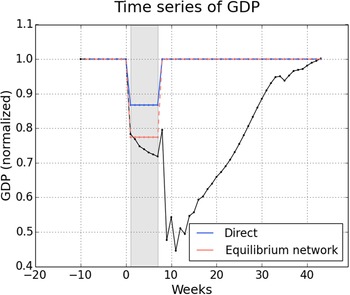
Figure 2 presents the time series of GDP after a 7-week lockdown beginning at the time step indexed by zero.Footnote 8 The dotted horizontal blue line marks the GDP after deducing the direct cost of the lockdown. The dotted horizontal salmon line marks the GDP after incorporating the network effects that follow from the direct impact within an equilibrium framework. The black line marks the time series of GDP generated by our disequilibrium model in response to the lockdown shock. The figure shows that the decline in GDP begins at the first time step after the lockdown. GDP continues to decline at each time step in the lockdown and for some time steps after the end of the lockdown.
The decline in GDP at the first time step of the lockdown reflects the immediate impact of the lockdown, which arises from firms not being allowed to produce as much as during normal times. The decline in GDP after the first time step reflects network effects. Where by “network effects,” we mean the fact that a decline in the output of some firms at one time step generates a decline in the output of other firms in the following time step in so far as the second set of firms use the output of the first set of firms as an input into their own production process. The decline in output of one firm because of the decrease in the output of another percolates through the production network, thereby generating a decline in GDP for several time steps into the lockdown and even beyond the lockdown period. For one set of parameter values, weekly GDP at its lowest level after lockdown reaches
 $49\%$
of the pre-lockdown level. At its lowest, disequilibrium GDP is about
 $27$
percentage points less than the equilibrium GDP and about
 $37$
percentage points less than the GDP after deducting the direct impact.
The response of GDP to the COVID lockdown shock. Parameters:
 $\phi =0.1, \rho =0.9, \sigma =-1$
. The lockdown shaded in gray extends from week
 $1$
to week
 $7$
.

Remark 4 (The second dip in GDP). Note the second dip in GDP at the second time step after the lockdown is lifted. The reason for the second dip is as follows. During the lockdown, firms are constrained both in terms of how much intermediate inputs they demand and how much output they supply. The household is not constraint in terms of how much final goods it can demand (though it does experience a decrease in wages). The market for intermediate goods is therefore more constrained by the lockdown (from the demand and supply side) than the market for final goods. When the lockdown ends, the market for intermediate goods rebounds by absorbing resources away from the market for final goods. Put differently, firms direct a greater share of resources towards firms that produce predominantly for intermediate use, or equivalently they direct resources away from the household and from firms that produce predominantly for final consumption. This temporary reallocation of resources away from the market for final goods registers itself as a second dip in GDP. The large dip in GDP occurs at the second rather than the first time step after the lifting of the lockdown. This is because in the first time step after the lockdown the decline in inventory accumulated over the lockdown period is sufficient to compensate for the increase in demand for intermediate inputs. However, in the second and following time steps, further declines in inventory do not prove sufficient, and therefore the increase in intermediate inputs comes at the expense of a decrease in final goods. Note that the second dip in GDP is a part of the process of recovery of the economy since present increases in intermediary goods generates future increases in final goods. One may therefore view the second dip as the cost of “kickstarting” the economy.Footnote 9
Figure 3 plots the share of goods produced at each time step that is used as intermediate inputs. The share of intermediate goods declines sharply upon the imposition of the lockdown. The decline occurs because at the first time step of the lockdown firms are impacted by the lockdown constraint, but the household is not constraint in spending wages earned in the previous period. From the second time step of the lockdown onwards, the household too is affected by the lockdown albeit indirectly due to unemployment. This means that, from the second time step of the lockdown onwards, the household is not able to purchase as large a share of goods as in the first time step of the lockdown, thereby generating a mild increase in the share of intermediate goods as compared to the first time step of the lockdown. The share of intermediate inputs increases sharply immediately upon the lifting of the lockdown, because firms are able to outbid the household as the quantity constraint on firms is lifted. This advantage of the firms vis-a-vis the household dissipates in following time steps as the benefits of the removal of quantity constraints percolate to the household in several ways including an increase in employment.
The response of share of intermediate goods to the COVID lockdown shock. Parameters:
 $\phi =0.1, \sigma =-1$
. The lockdown shaded in gray extends from week
 $1$
to week
 $7$
.

Naturally, the production network amplifies the direct impact of the lockdown. This occurs through a decrease in the availability of intermediate inputs and an endogenous increase in the job separation rate. We compute a network multiple to measure the amplification of the direct impact of the lockdown through disequilibrium network dynamics. We define the network multiple (
 $\omega$
) as:
 \begin{equation} \omega =\frac{1-y_{\min}}{1-y_{\text{direct}}} \end{equation}
where
 $y_{\min}$
is the minimum GDP after the lockdown and
 $y_{\text{direct}}$
is the GDP considering only the direct effect of lockdown.
 $y_{\min}$
and
 $y_{\text{direct}}$
are normalized to the pre-shock GDP. This means that the network multiple is
 $1$
when the direct impact equals the full impact.
 $y_{\text{direct}}$
was earlier computed to be 0.875. Figure 4 presents the network multiple
 $\omega$
for different values of the weekly job-finding rate. Network multiple
 $\omega$
varies from
 $2.8$
to
 $5.3$
for weekly job-finding rates between
 $0.05$
and
 $0.2$
, with high network amplification ratios corresponding to low job-finding rates. Note that the network multiple declines with an increase in the job-finding
 $\phi$
, that is, the labor dynamics amplify the network effects. At full employment
 $\phi =1$
, the network multiple
 $\omega$
is approximately
 $2.2$
. The network multiple at full employment indicates the amplification of the direct lockdown shock solely through changes in the availability of intermediate inputs. We use the value of the network multiple
 $\omega$
at
 $\phi =1$
to measure the share of the network amplification that comes from the disequilibrium unemployment effect. For instance, when the weekly job-finding rate
 $\phi =0.2$
, the network multiple
 $\omega$
is about
 $2.8$
, of which
 $2.2$
comes from the disequilibrium dynamics of intermediate inputs. Therefore, about three-fourths of the disequilibrium network amplification of the lockdown shock comes from the dynamics of intermediate inputs and the remaining one-fourth from disequilibrium unemployment. The share of unemployment dynamics in network amplification increases with a decrease in the job-finding rate, with the job-finding rate
 $\phi$
accounting for nearly three-quarters of the total amplification when it is
 $0.05$
.
The amplification of the direct lockdown shock through the production network. Parameters:
 $\rho =0.9, \sigma =-1$
.

Figure 5 plots the average rate of unemployment in Q2, Q3, and Q4 of 2020. We include 6 of the 7 weeks of lockdown in Q2. The rate of unemployment decreases with the weekly job-finding rate. For a weekly job-finding rate of 5–20% and an endogenously determined job-separation rate, the average unemployment rate for Q2–Q4 2020 lies in the 15–40% range. Figure 6 presents the cost of the lockdown as a proportion of annual GDP for different values of the job-finding rate. The cost is measured as the difference between weekly GDP and equilibrium GDP for each week till the US economy reaches the post-shock equilibrium. The cost declines with an increase in the job-finding rate. This is simply because a higher job-finding rate generates greater employment, which means more labor is available to produce output. The cost of the lockdown varies between 10% and 33% of annual GDP, with the exact cost depending on the job-finding rate. Hall (Reference Hall>2005, pp. 115–122) reports that the monthly job-finding rate is in the 10–50% range. This means that the weekly job-finding rate is in the 3–15% range. With a weekly job-finding rate of
 $5\%$
, the lockdown would cost the US economy about third of annual GDP, whereas with a weekly job-finding rate of
 $10\%$
the cost decreases to half as much.Footnote
10
Unemployment rate for different values of weekly job-finding rate. Parameters:
 $\rho =0.9, \sigma =-1$
.

Cost of the lockdown for different values of weekly job-finding rate. Parameters:
 $\rho =0.9, \sigma =-1$
.

5. Sensitivity analysis with respect to price stickiness
In this section, we investigate the sensitivity of our results with respect to exogenously given price stickiness. We then introduce a new form of endogenously heterogeneous price stickiness and study the sensitivity of our model with respect to it.
Cost of the lockdown for different values of price stickiness. Parameters:
 $\phi =0.1, \sigma =-1$
.

5.1. Sensitivity to the speed of price adjustment
Figure 7 shows that the cost of the lockdown has a non-monotonic relation with price stickiness. More specifically, the cost decreases with an increase in price stickiness for a large range of values and then increases when price stickiness crosses a certain threshold. In the disequilibrium dynamics generated by the model, the greater the flexibility of prices, the greater the changes in relative prices. Such changes in prices generate temporary increases in the output of some firms and temporary decreases in output of others. When the job-finding rate is less than 1, the firms which decrease output release labor, all of which is not instantaneously absorbed by firms which are in a position to expand output. In other words, relative price changes in the out-of-equilibrium phase act as endogenous shocks generated by the interactions between firms. These endogenous shocks generate unemployment in the absence of perfect labor mobility from one firm to another. Price stickiness dampens these endogenous shocks and thereby decreases the unemployment generated by the shocks. This means more labor is used in producing output, thereby generating a negative relation between the cost of the lockdown and the stickiness of prices for a certain range of values. The reason for why the cost of the lockdown increases when price stickiness crosses a certain threshold is more conventional, that is, a certain quantum of price flexibility is needed for firms to adapt to changing availability of intermediate inputs.Footnote 11
Remark 5 (The stabilizing effect of price stickiness in a network economy). The U-shaped relation we find between price stickiness and the economic impact of the COVID lockdown is related to an intriguing literature which questions conventional beliefs about macroeconomic consequences of price flexibility. The literature began with De Long and Summers’ (Reference De Long and Summers>1986) claim that an increase in price stickiness explains the post-War decline in aggregate volatility. Their basic line of reasoning is as follows. Greater flexibility can generate a rapid decline in the price level in response to a negative aggregate demand shock. Such declines in the price level can trigger an expectation of future deflation and thereby increase the real rate of interest, which in turn can aggravate the impact of the demand shock on economic activity.Footnote 12 This mechanism works through the impact of the flexibility of the price level on real wages and real interest expectations. Our mechanism in contrast works through the impact of the flexibility of relative prices on the interrelated decisions of firms in a high-dimensional economy. In essence, we have pointed to a whole new mechanism through which price stickiness can aid the stability of an economic system particularly as the system reconfigures in response to a shock.
Finally, we remark on the relation between price stickiness and the size of the large second dip in GDP which appears in Figure 2. We measure the second dip as the difference between GDP at the last time step of the lockdown and the second time step after the lifting of the lockdown. As shown in Figure 8, the lower the rigidity of prices, the greater the size of the second dip. Price rigidity limits the ability of firms to respond to the relaxation of the lockdown. More specifically, firms draw resources towards themselves—and away from the household—by bidding up prices. Price rigidity limits such increases in prices and therefore limits the quantum of resources bid away from the production of final goods after the relaxation of the lockdown. And by limiting the diversion of resources to the market for intermediate goods, price rigidity limits the decline in final goods (GDP) in response to the end of the lockdown restrictions.
The size of the sharp decline in GDP immediately after lifting of the lockdown for different values of price stickiness. Parameters:
 $\phi =0.1, \sigma =-1$
.

5.2. Endogenously heterogenous price stickiness
We introduce heterogeneity in price stickiness to test for its significance in determining the cost of the lockdown. More specifically, each firm
 $i$
changes its price at a given time step
 $t$
with probability
 ${\phi }_{i}^{t}$
given by:
 \begin{equation} {\phi }_{i}^{t}=\left(\frac{{\kappa }_{i}^{t}}{1+{\kappa }_{i}^{t}}\right)^{\psi } \end{equation}
where
 $\psi \geq 0$
is a scaling parameter and
 ${\kappa }_{i}^{t}=\frac{| {p}_{i}^{t-1}-{\overline{p}}_{i}^{t}| }{{p}_{i}^{t-1}}$
with
 ${\overline{p}}_{i}^{t}$
denoting the market clearing price. The pricing schema noted in equation (27) means that firms that experience a greater gap between their demand and supply are more likely to change prices, therefore generating an endogenous heterogeneity in the probability of price change across firms and over time. Figure 9 shows the relation between the sensitivity parameter
 $\psi$
and the cost of the lockdown. Note that the lockdown generates a sizeable cost even with heterogeneous price stickiness. Furthermore, the y-axis of the figure shows that the cost of the lockdown does not vary sizeably with the sensitivity parameter
 $\psi$
.Footnote
13
The cost of the lockdown for different heterogeneity in the stickiness of prices. Parameters:
 $\phi =0.1, \sigma =-1$
.

6. Concluding thoughts
In this paper, we presented a network economy model which sheds light on the dynamics of an economic system when it goes out of equilibrium in response to a real shock. We believe that such models are particularly useful to study the economic dynamics which will follow from the COVID lockdowns. We calibrated the model to a data set on buyer–seller relations between firms in the US economy so as to estimate the impact of the lockdown. Our estimates suggest that the impact of the lockdown on GDP and unemployment is likely to be comparable to that of the Great Recession and the Great Depression. The unemployment rate of the US economy in 2020 may well be the highest reported since the Great Depression of 1929. Disequilibrium dynamics within a network economy is capable of doubling or tripling the direct cost of the lockdown.
Our estimates are based on limited network data and therefore must be read with caution. We estimated the cost of the lockdown by calibrating the model using a data set with about
 $10^{5}$
firms. In reality, the US economy has on the order of
 $10^{6}$
firms and perhaps
 $10^{8}$
buyer–seller relations (Axtell, Reference Axtell>2001). Though our data set contains more information than the input–output table, it omits vast majority of firm-to-firm transactions in the US economy. Our model suggests that these firm-to-firm transactions along with liquidity constraints are likely to be significant drivers of the dynamics of GDP and unemployment. Another empirical limitation of ours is that the sectoral distribution of firms within our data set is not identical to that of the US economy. Insofar as the lockdown shock is heterogeneous in its impact on sectors, the differences in sectoral representation between our data set and the US economy are likely to matter.
With sufficient data, models of the kind presented in this paper can become a reasonable alternative to econometric impulse response models. Granular representations of high-dimensional distributed systems are useful when structural parameters that guide econometric models are likely to become unstable in response to shocks. The stability of the structural parameters of low-dimensional models depends on stable relations between microeconomic entities, or equivalently on the canceling of diverse changes in the relations between microeconomic entities in response to shocks (Stock and Watson, Reference Stock and Watson>1996). We have shown how the relations between microeconomic entities defined by the flows of goods and money between them can change in response to an exogenous shock. Furthermore, the afore-noted micro changes have cumulative and temporal effects as the disequilibrium spills over from one market to another. These are sufficient reasons to expect the structural parameters of reduced form models to change in response to the lockdown shock. While high-dimensional models present a viable alternative in such circumstances, their empirical usefulness will depend on the granularity of data using which the models are calibrated.
We made numerous simplifying assumptions so as to illustrate the basic mechanisms at work within our model. Not the least of which is the assumption that after the COVID lockdown the economy returns to an equilibrium which is identical to the pre-COVID equilibrium. Such a return is unlikely in the light of adaptive behavior by firms due to the virus itself and novel policy risks. Firms are less likely to source inputs from regions more prone to the closure of movement of goods in response to pandemics. There may also be a change in make-or-buy decisions, whereby firms decide to vertically integrate so as to get more direct command over the availability of key inputs. Not only the structure of the production network, but its granularity too may change in the aftermath of the virus and policy response to the virus. The long-term cost of the lockdown therefore must incorporate changes in the production structure that emerge from firms’ adapting to new policy risks. Lastly, our analysis did not incorporate the impact of the pandemic on consumer preferences and other determinants of the demand for final goods.
Despite its many limitations, models of the kind developed in this paper present an alternative to comparative statics that are in earnest of little use in understanding the COVID crisis. After shocks as large as the pandemic and the policy response to the pandemic, the economic system takes time to traverse to a new equilibrium. Comparative statics exercises simply assume away that which is of greatest—dare we say of sole—interest. In short, there are serious pragmatic motivations which call upon improving the empirical limitations of disequilibrium network models like the one presented in this paper.
Postscript
The estimates of the cost of lockdown presented in this paper were generated in June 2020. More than a year has passed since. It is therefore sensible to discuss the accuracy of our predictions, and the sources of discrepancy when compared to reality. This exercise is particularly fruitful insofar as the sources of the discrepancy are theoretical factors that have been overlooked. Understanding such theoretical sources of discrepancy will help with making more appropriate modeling choices in the future. Now to get to the matter, according to FRED data, the decline in US GDP in Q2, Q3, and Q4 of 2020 was about 9.5%, 1.7%, and 1.2% respectively. Therefore, the cost of the lockdown in terms of annual GDP is approximately 3.1% of GDP.
Within our setting, the cost of the lockdown in case of full employment (with a job-finding rate
 $\phi =1$
) is about
 $3.9\%$
of annual GDP, which is nearly equivalent to the empirically observed magnitude. Our model is sensitive to unemployment dynamics, therefore as we decrease the job-finding rate, the cost of the lockdown increases sizeably. For instance, a weekly job-finding rate of
 $50\%$
implies a cost of 5% of annual GDP. Note that the observed mean rate of unemployment in the USA was about 8.7% in the post-lockdown months of 2020. Working backwards, our model generates the observed rate of unemployment with a weekly job-finding rate of
 $33\%$
. When the model is calibrated to the correct rate of unemployment, the cost of the lockdown in terms of annual GDP is approximately
 $6\%$
. This is roughly twice the observed cost of the lockdown.
We had sizeably overestimated the cost of the lockdown because we overestimated the level of unemployment caused by the lockdown. Using data on monthly job-finding rates, we took the weekly job-finding rate to be about 10% percent, which in turn generated a cost of about
 $18\%$
of annual GDP. In hindsight, it is evident that we had overlooked an important theoretical matter with respect to the labor market process in the aftermath of the lockdown. More specifically, we assumed that the job-finding rate after the lockdown will be similar to that during ordinary times. This is unlikely to be true. In fact, the job-finding rate after the lockdown is likely to sizeably greater than usual. Under ordinary circumstances, the labor market is riddled with the problem of reallocating workers from one firm to another and from one sector to another, as market activity responds to changes in primitives like technology and preferences. The COVID lockdown is not equivalent to permanent changes in technology and preferences. Therefore, much of the flux in the labor market is likely to reflect a temporary separation of workers from firms and industries in which they were employed before the lockdown. And job-finding rates are likely to be sizeably greater when an economy goes back to the old equilibrium after a temporary perturbation as compared to an economy trying to find a new equilibrium in response to a permanent change in primitives.
There are three more reasons for why our model overestimated the cost of the lockdown. The first of which is intertemporal substitution of labor. Workers may have supplied more hours of labor after the end of the lockdown than they would under ordinary circumstances. This is because they consumed more leisure during the lockdown than under ordinary circumstances. Rational labor-leisure choice, with say a yearly horizon, would tend to generate such behavior. The increase in labor supplied in the post-lockdown period would generate faster recovery than predicted by our model in which the total quantity of labor is fixed. The second reason why our model overestimated the cost of the lockdown has to do with the fact that the lockdown was not implemented equally rigorously across all states in the USA. Moreover, there was some heterogeneity in the entry and exit of different states from the lockdown. We had implicitly assumed an equally stringent lockdown across all states in the USA. This means that we did not incorporate the that fact that production may have temporarily shifted from one state to another as states entered and existed the lockdown. The third reason for why our model overestimated the cost of the lockdown has to do with the size of the direct shocks applied to the model. We assumed that nearly all of the impact of the lockdown on output in March was ascribable to direct effects as network effects are likely to take time to set in. In fact, when we reduce the size of direct shock to
 $70\%$
of what we applied, the model generates almost exactly the observed cost of the lockdown for the observed rate of unemployment. There is therefore a need to supplement theoretical network models of the kind presented in this paper with out-of-equilibrium econometrics which can distinguish direct effects from network effects. Such econometric work will allow for the application of the right-sized exogenous shock to network models which amplify the shock.
It must be said that with the calibration presented in this paper, we were unlikely to have accurately estimated the cost of the lockdown. Not the least of which is because the network data are terribly incomplete and in no way sufficiently representative of the US economy. Our purpose was merely to illustrate the possibility of developing a synthetic economy in silico, which would exhibit the disequilibrium dynamics that an economy would go through after a large shock. The calibration exercise was meant to illustrate the possibility of granular-tuning of such models to network data, which when sufficiently representative of the economic system as a whole can transform the model into a testbed for policy experiments.
Appendix A: Accounting for GDP in a network economy model
Any procedure of accounting for GDP within an economic model involves the pursuit of three distinct objectives. The first of which is “model-consistency,” that is, the procedure must be consistent when viewed from the point of different ingredients of the model. For instance, in the context of an economy capable of exhibiting disequilibrium dynamics, it would be problematic to value some items at equilibrium prices and others at current prices. The second goal is “national income accounting consistency or NIA-consistency,” that is, the procedure must incorporate a reasonable mapping between accounting within the model and the mechanical aspects of national income accounting. For instance, in so far as “net exports” are a part of GDP according to national income accounting norms, they must be part of GDP within the model setting too. The third goal is “economic consistency,” that is, the procedure must reflect the economic rationale beneath national income accounting. This means that as to whether or not a variable generated by the model is included in GDP must depend not merely on its “label” but on the processes by which it is generated within the model and as to whether these processes are consistent with the economic rationale for their inclusion from the national income accounting point of view.
Unfortunately, the joint pursuit of the three objectives can be difficult within a network setting, and particularly so if the network economy is capable of exhibiting disequilibrium dynamics. In certain circumstances, each of the three criteria of consistency may present a different answer to the question of whether and how a variable is to be included in GDP. The question of inventory within our model is illustrative. Within our model, firms can face negative excess demand when prices are sticky, in which case they carry the unsold output to the next period. More specifically, the unsold output generated at the beginning of period
 $t$
is added to the new output produced at the end of period
 $t$
, and the two together are carried to period
 $t+1$
without distinguishing between unsold output and newly produced output. Suppose we use the “expenditure method” for computing GDP.Footnote
14
According to national income accounting rules, changes in inventory are a part of GDP; therefore, “NIA-consistency” would require changes in inventory to be included in GDP. But including changes in inventory to GDP does not sit well with the pursuit of “economic consistency.” Within national income accounting framework, the rationale for including changes in inventory in GDP is that value-added should be assigned to the period in which it occurred (BEA, >2006, Chapter 7). A positive change in inventories means that total production exceeded final sales, and that the excess was accumulated as inventory. Therefore, in so far as GDP is to reflect value-added in the current period, positive changes in inventory should be added to final sales and negative changes in inventory should be deduced from final sales while accounting for GDP.
The rationale for including changes in inventory in GDP suggests that the item labeled as “inventory” within our model does not qualify to be included within GDP. Put differently, the second and third criteria provide different answers to the question of whether changes in the variable labeled as “inventory” within our model should be included in GDP. To understand the reason for this discrepancy, consider a linear network economy or supply chain, wherein resources flow from higher-order (upstream) firms to lower-order (downstream) firms to retail firms. For analytical simplicity, assume away the possibility that higher-order firms use lower-order goods as inputs into their production process. Put differently, goods cannot flow backwards from lower-order firms to higher-order firms. In equilibrium, such an economy will exhibit a constant level of inventory for each firm (though the contents of the inventory may be drawn-down and replenished at each time step).Footnote 15 Suppose the economy is hit by an exogenous shock because of which it temporarily exhibits disequilibrium dynamics. Once disequilibrium sets in, the level of inventory of the firms will change and this change in inventory—whether positive or negative—must be included in GDP so that GDP reflects current value-added.
Matters are however wholly different if we do away with the assumption that goods flow in one direction within the network economy. More specifically, suppose some higher-order firms purchase part of their inputs from some lower-order firms, that is, the economy is a large network system with a whole complex of connections between firms rather than a simple linear system. When such a network economy is hit by an exogenous shock, it too will exhibit positive and negative changes in the level of inventories. However, these changes cannot be readily accounted for as the value-added in the current time step. This is because the excess inventory accumulated at the current time step (i.e. a positive change in inventory) may be drawn by higher-order firms in the succeeding time steps. The excess accumulation of inventory, therefore, contributes to the destruction of value amidst disequilibrium as resources may be drawn from lower-order firms to higher-order firms. To use an example, an increase in the inventory of automobiles reflects value-added in so far as the automobiles are on their way to the final consumers, the increase in inventory does not reflect value-added if they are going to be purchased by smelters who will convert them again into iron ore. Similarly, the accumulation of any intermediate good reflects value-added only in so far as the accumulated inventory will follow its usual path, however circuitous, to the final consumer. If the excess accumulation of inventory will be torn down by higher-order firms as part of the disequilibrium reflux, then the change in inventory does not reflect “value-added” in the sense of an increase in the value of resources from the point of view of final consumption.
Our network economy is not a linear supply chain, rather firms purchase from other firms through a myriad of linkages. Lower-order firms can supply inputs to higher-order firms.Footnote 16 Furthermore, the share of goods produced by lower-order firms that go to higher-order uses depends on relative prices. This means that prima facia economic rationale dictates that one cannot simply include the item labeled as changes in inventory within the model to GDP, rather one must carefully examine the exact nature of the disequilibrium and the temporary flows of the accumulated inventory.Footnote 17 The disequilibrium introduced by the lockdown shocks studied in this paper is a case in point. The imposition of the lockdown generates a steep accumulation of inventory and the lifting of the lockdown generates a sharp decline in inventory. Much of the inventory accumulated during the lockdown, however, does not move downstream after the lifting of the lockdown, rather it moves upstream as higher-order firms outbid lower-order firms. Therefore, the disequilibrium accumulation of inventory did not reflect a mere road block on the way to final consumer, that is, it was not merely the building up of a wave of “near-final goods” temporarily halted from the final consumer. In using the expenditure methods, we therefore do not include such changes in inventory as a part of GDP. Rather we limit GDP to the goods purchased by final consumer, since there is no government, internal trade, or investments within the model. Naturally, our treatment of changes in inventory is not without problem. Unfortunately, this is an area where all solutions are at best second-best.
Appendix B: Convergence
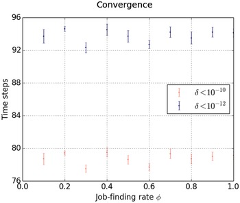
Figure 10 shows that the model has robust properties of convergence towards equilibrium. Convergence is measured by the mean absolute price change
 $\delta ^{t}=\frac{1}{n}{\sum }_{i=1}^{n}\frac{| {p}_{i}^{t}-{p}_{i}^{t-1}| }{{p}_{i}^{t-1}}$
. The y-axis marks the time steps necessary for
 $\delta ^{t}$
to go below
 $10^{-10}$
and
 $10^{-12}$
.
Number of time steps necessary for the economy to converge for different values of the job-finding rate
 $\phi$
. The job-finding rate varies from
 $0.1$
to
 $1$
with increments of
 $0.1$
. The figure presents the mean and standard error of
 $10$
computational experiments for each value of the job-finding rates. The number of firms
 $n$
is fixed at
 $1000$
.

B.1. Sectoral distribution of firms
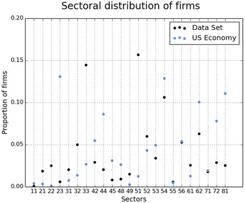
Figure 11 presents the sectoral distribution of firms in our data set and in the US economy as a whole. The sectoral distribution of firms in the US economy is plotted using year 2007 data from the Small Business Administration on 6,116,071 entities. Note that for some sectors like NAICS 33 [Manufacturing] there are sizeable differences between the share of firms in our data set and in the US economy, whereas in other sectors like NAICS 53 [Real Estate Rental] the differences are less pronounced. In sectors like NAICS 71 [Arts, Entertainment and Recreation], the proportion of firms in our data nearly coincides with that in the US economy.
The distribution of firms across different sectors within our data set and in the US economy. The x-axis marks two-digit NAICS codes.

Appendix C: Input complementarity: CES exponent
$\sigma$

Figure 12 shows that the cost of the lockdown decreases with an increase in the CES exponent
 $\sigma$
, or equivalently the cost of the lockdown decreases with a decrease in the complementarity between inputs. This is for obvious reasons.
The cost of the lockdown for different degrees of complementarities between intermediate inputs. Parameters: weekly job-finding rate
 $\phi =0.1$
and price stickiness
 $\rho =0.5$
.

Appendix D: Size of lockdown
Figure 13 presents the cost of the lockdown for different sizes of the lockdown, where the size of the lockdown is some multiple of the empirical distribution of the lockdown. The motivation for these simulations is the fact that our lockdown shock ultimately does not come from granular empirical data on which firms have to reduce capacity or cease production by government mandate. We therefore test the robustness of our results giving each firm a shock which is a multiple of the shock computed using sectoral data, with the multiple ranging between 0.5 and 1.4. Unsurprisingly, Figure 13 shows that as the size of the lockdown shock increases, so does the cost.
The cost of the lockdown for different sizes of the lockdown shock. Parameters: weekly job-finding rate
 $\phi =0.1$
and price stickiness
 $\rho =0.5$
.

Appendix E: Disequilibrium unemployment
In this section, we illustrate the basic dynamics by which unemployment emerges within the model. To this end, we implement an idiosyncratic productivity shock after the economy converges to equilibrium. We report the changes in firms’ sizes and the resulting unemployment as the economy exhibits disequilibrium dynamics in response to the shock. Each experiment involved a one-time idiosyncratic productivity shock after the economy reached equilibrium. More specifically, we modify each firm’s production to the following by including the term
 $A_{i}$
:
 \begin{equation} f_{i}\!\left(l_{i},\left(y_{ij}\right)_{j=1,\ldots,{n_{i}}}\right)=A_{i}k_{i}\!\left(M\right){l}_{i}^{\alpha }\!\left(\sum _{j\in S_{i}(M)}{y}_{ij}^{\sigma }\right)^{\frac{1-\alpha }{\sigma }}a \end{equation}
where
 $A_{i}$
marks productivity. We implement an idiosyncratic productivity shock in the following manner: each firm
 $i'$
s productivity
 $A_{i}$
changes to
 $\varepsilon _{i}A_{i}$
at the time step indexed by 0, where
 $\varepsilon _{i}$
is drawn from a lognormal distribution with mean
 $1$
and standard deviation
 $\gamma$
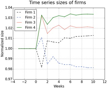
. We record the disequilibrium dynamics in unemployment as the shock propagates through the production network from one time step to another. Figure 14 shows the time series of the sizes of four firms after an idiosyncratic productivity shock at time step zero. The size of each firm is normalized to its pre-shock equilibrium value. The sizes of all four firms change in response to the productivity shock. Some firms contract at some time steps. Note that firms sizes do not move monotonically to their new equilibrium values, rather firms’ sizes fluctuate non-monotonically, with the amplitude of the fluctuations decaying as the economy converges to the new equilibrium. The fluctuations in firms sizes can be such that a firm whose post-shock size is greater than the pre-shock size exhibits a temporary decrease in its size, see for instance Firm
 $1$
in Figure 14. Similarly, a firm whose post-shock size is smaller than its pre-shock size can exhibit a temporary increase in its size, see for instance Firm
 $2$
in Figure 14.
Time series of firm sizes after a real shock. Parameters:
 $n=10^{4}, \gamma =0.1, \phi =0.1$
.

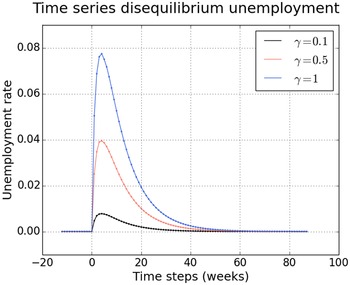
Time series of disequilibrium unemployment. Parameters:
 $n=10^{3}, \phi =0.1$
.

Variation in unemployment with the standard deviation of idiosyncratic productivity shocks. Parameters:
 $n=10^{3}, \phi =0.1$
. The figure reports results from
 $100$
experiments for each value of
 $\gamma$
ranging from
 $0$
to
 $10$
with increments of
 $0.05$
. The figure plots all
 $100$
observations for each parameter value.

The fluctuations in firms’ sizes on the path to equilibrium emerges from complex dependency of the size of each firm on the decisions of other firms with whom it shares direct and indirect network relations. A firm’s size at time step
 $t+1$
depends on the sizes of its output buyers at
 $t$
and their decision on how much to spend on the firm. The decision of the output buyers on how much to spend on a given input seller depends on the prices of all inputs. Such interdependencies can generate non-monotonic movements in firms’ sizes. More generally, the decisions of a firm at time step
 $t$
depends on the decisions of its input sellers at
 $t-1$
and its output buyers at
 $t$
. However, this means that the decisions of a firm at time step
 $t$
depends on the decisions of the input sellers of its input sellers at
 $t-2$
and will influence the decisions of its output buyers at
 $t+1$
. More generally, local market clearing depends on the alignment of the decisions of firms that are directly connected. General equilibrium however requires the alignment of decisions of all firms in the economy. Firms respond to the decisions of firms removed from them by
 $k$
degree by a lag of
 $t+k$
time steps. Therefore, it takes time for the economy to reach the new equilibrium through decentralized interactions.
Figure 15 shows the time series of unemployment after an idiosyncratic productivity shock for three different values of the standard deviation of the distribution from which the shocks are drawn. Higher values of standard deviation generate greater unemployment at each time step in the transition from one equilibrium to another. Figure 16 presents the average unemployment rate in the first quarter after an idiosyncratic productivity shock for different sizes of the standard deviation of the distribution from which the shock is drawn. The figure reports results from
 $100$
experiments for values of
 $\gamma$
ranging from
 $0$
to
 $10$
with increments of
 $0.1$
. The figure plots mean values from the
 $100$
experiments for each value of
 $\gamma$
. Figure 16 shows that the rate of unemployment increases with the standard deviation of the distribution of idiosyncratic productivity shocks. The reason for the positive relation between the unemployment rate and the variance of idiosyncratic productivity shocks is as follows. The greater the variation in firms’ productivity, the greater the probability that a firm’s post-shock equilibrium size will be significantly different from its pre-shock equilibrium size. The firms whose post-shock equilibrium size is smaller than the pre-shock equilibrium size will release labor as they transition to the new equilibrium. The quantity of labor so separated from their jobs depends on the number of firms who experience sizeable declines in their equilibrium sizes. Productivity shocks with greater variance therefore increase unemployment by increasing the number of firms who experience sizeable declines in their equilibrium sizes. The results of our investigations can be summarized as follows:
Result 1 (Unemployment). The propagation of real shocks within a network economy can generate a temporary increase in the unemployment rate through a temporary increase in the job-separation rate. The increase in unemployment rate is positively related to the heterogeneity of the real shock.