1. INTRODUCTION
The problem of deflecting near-Earth asteroids (NEAs) to mitigate their probable impacts upon the Earth has attracted a lot of attention in recent years. One feasible deflection strategy is to send a group of small spacecraft into the proximity of the NEAs to execute an intervention. Due to the huge distance from the Earth to the asteroid, autonomous orbit determination using only on board measurements provides a potential way to avoid the interruption from ground tracking and communication over-crowding problems of the Deep Space Network (DSN). Precise navigation is a key technology for asteroid deflection missions because the target bodies are fairly small in size and highly irregular in shape and their physical characteristics cannot be exactly observed. An orbit determination method is required to provide accurate position and velocity information of the spacecraft to satisfy the requirements for implementing the mitigation strategies. This paper investigates an autonomous orbit determination method for a two-spacecraft formation flying under control with a slowly rotating NEA.
Many investigations have been made into deep space orbit determination methods. Thornton and Border (Reference Thornton and Border2002) introduced orbit determination techniques for deep space navigation such as Earth-based tracking, range and Doppler tracking, Very Long Baseline Interferometry (VLBI) tracking and radiometric tracking. Chung (Reference Chung2006) developed several orbit determination methods for a deep space Laser Interferometer Space Antenna (LISA) mission. DSN range and range rate, VLBI angel tracking data and inter-spacecraft range and range rate observations were processed to determine the orbits of the spacecraft. Due to the high cost of using DSN and the low precision and time delay in the communication transformation, autonomous orbit determination methods have been closely examined, especially for deep space missions. Ray et al. (Reference Ray, Sheikh, Graven, Wolff, Wood and Gendreau2008) described deep space navigation using celestrial X-ray sources. Li and Peng (Reference Li and Peng2011) described Mars entry navigation using an inertial measurement unit (IMU) and orbiting or surface radiometric beacons. Ma et al. (Reference Ma, Fang and Ning2013) surveyed autonomous navigation technology in deep space missions.
Among the known deep space orbit determination methods, optical orbit determination methods can obtain high precision by means of observing azimuth and elevation and taking images of the target bodies, and a number of papers have been published which propose optical observation. An orbit determination method based on the Sun Line of Sight (LOS) vector measured by an on board camera was an optional strategy employed in the Deep Impact mission (Cui et al., Reference Cui, Chang and Cui2010). Moreover, the on board navigation camera has proved to be a useful sensor for feature tracking for small body exploration missions (Johnson and Matthies, Reference Johnson and Matthies1999), and for pinpoint landing technology (Li et al., Reference Li, Cui and Cui2006; Li et al., Reference Li, Cui and Cui2007; Trawny et al., Reference Trawny, Mourikis, Roumeliotis, Johnson and Montgomery2007). Maddock (Reference Maddock2010) studied the navigation problem of a formation of solar concentrators for asteroid deflection by using the on board camera. Dionne (Reference Dionne2009) presented an improved autonomous optical navigation method using range measurement for a spacecraft in orbit about an asteroid. However, the dynamic equations in his work were too simple to describe the spacecraft dynamic environment accurately.
This paper extends the work presented by Vetrisano et al. (Reference Vetrisano, Yang and Vasile2012) and focuses on relative orbit determination for a spacecraft-asteroid formation, which utilised two spacecraft flying in formation with a slowly rotating asteroid about one km distant with the asteroid considered to be the central body of the formation. The extended work includes the dynamics and control strategy in the aspects of the definitions of the coordinate systems, the dynamics modelling and the spacecraft motion with the real orbital parameters under perturbations and control efforts. The dynamics of the spacecraft-asteroid formation is studied taking into account the perturbations of the Sun and the asteroid. An improved combination model of spacecraft-to-asteroid observations with inter-spacecraft communication coming from the on board high-resolution camera aided with range measurement is used to determine the relative orbits of the spacecraft to the asteroid. Although the optical camera and Light/radio Detecting And Ranging (LIDAR) integrated navigation is not a new technology, there is a new challenge to use these measurements in asteroid deflection missions because of the uncertainty and complication in the small body's dynamic environment. Different combinations of multiple measurements compose different orbit determination scenarios. According to Vetrisano and Vasile (Reference Vetrisano and Vasile2012), an Unscented Kalman Filter (UKF) algorithm is used to fuse the measurements from each spacecraft. In the present work, only the relative position and velocity of the spacecraft with respect to the asteroid are estimated, the attitude is considered to be known from the star sensor and not studied.
According to Psiaki's (Reference Psiaki1999) work, an autonomous orbit determination algorithm was designed to simultaneously determine the orbits of two spacecraft by making measurements of the relative position vector from one spacecraft to the other. This concept gives a reference to design a filter in this work. For the highly non-linear system state estimation problem, the UKF has a better performance than an Extended Kalman Filter (EKF), because the former provides at least second-order accuracy compared to the first-order accuracy of the later, while maintaining the same order of magnitude in computational complexity (Liu et al., Reference Liu, Kang, White, Ma and Tian2011; Oh and Johnson, Reference Oh and Johnson2007). Furthermore, the previous work of Vetrisano and Vasile (Reference Vetrisano and Vasile2012) has proved that the UKF techniques obtained the best performance in fusing the multiple measurements. As a consequence, a nonlinear filtering technique based on UKF is used to autonomously determine the orbits of the formation and reconstruct the state of each spacecraft. Simulation results are analysed to validate the efficiency and the advantage of the proposed methods. Comparisons are made to indicate the sensitivity of different measurement types to the estimation solutions and demonstrate the benefit of adding the inter-spacecraft measurements to the measurement model.
The paper is organized as follows. Section 2 describes the dynamic model of the formation and designs the control law based on the Lyapunov control function. The measurement models are built up in Section 3. Section 4 introduces the different scenarios and describes the UKF algorithm. Section 5 shows the simulation results and comparative analyses. The final section summarises the major findings of the paper.
2. DYNAMICS AND CONTROL
This section describes the dynamics of the asteroid-spacecraft formation under the control force to propagate the state vectors of the spacecraft formation forward in time. It assumes that the position of the asteroid is known in the solar system according to observations from both spacecraft and ground station during the long interplanetary phase.
2.1. Dynamics Model of Spacecraft-Asteroid Formation
Before working on the dynamics of the formation, the related coordinate systems are defined (see Figure 1). Firstly, the Sun inertial coordinate system {O s-ijk} is defined. The origin is the centre of the Sun, the fundamental plane is the plane of the ecliptic, the i-axis directs to the Vernal equinox, the j-axis is perpendicular to the x-axis in the fundamental plane, and the k-axis points out perpendicularly with respect to the fundamental plane at the origin following the right-hand rule (Yim et al., Reference Yim, Crassidis and Junkins2000).
Geometrical relationship of the coordinate systems.

Secondly, the paper defines the asteroid rotating Hill reference frame O a-XYZ: the centre O a is the asteroid centre of mass. The (X,Y) coordinates define the relative orbit motion in the chief orbit plane. X-axis points out radially from Sun to the centre of mass of the asteroid, Y-axis is aligned in the direction of in-track motion, and Z-axis is normal to the orbital plane. The relative position and velocity of spacecraft with respect to the asteroid are described in this frame.
Thirdly, the spacecraft body frame o b–xbybzb is described which lies in the mass centre of the spacecraft. z b-axis is assumed to point to the centre of the asteroid. The y b-axis is anti-normal to the orbital plane and the x b-axis completes the dextral orthonormal frame.
Lastly, both the camera frame o c–xcyczc and the LIDAR frame o L-xLyLzL are considered to coincide with o b–xbybzb, for simplicity. When building up the dynamics model of the spacecraft-asteroid formation, the spacecraft is considered to be a point of mass.
Although most of the asteroids have a very irregular body shape, the gravitational potential generally can be modelled as a triaxial ellipsoid as expressed in Equation (1) with a, b and c the semi-axis dimensions (Dionne, Reference Dionne2009)
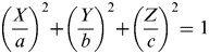 $$\left( {\displaystyle{X \over a}} \right)^2 + \left( {\displaystyle{Y \over b}} \right)^2 + \left( {\displaystyle{Z \over c}} \right)^2 = 1$$
where [X,Y,Z]T are the coordinates of the point on the surface of the asteroid. The gravity field of the asteroid is expressed as the sum of a spherical field plus a second degree and second order field (Hu and Scheeres, Reference Hu and Scheeres2002)
 $$U_{20 + 22} = \displaystyle{{\mu _A} \over {\delta r^3}} \left( {C_{20} \left( {1 - \displaystyle{3 \over 2}\cos ^2 \gamma} \right) + 3C_{22} \cos ^2 \gamma \cos 2\lambda} \right)$$
where μ A is the asteroid gravitational constant, C 20, C 22 are the spherical harmonic gravity coefficients, with
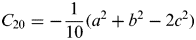 $$C_{20} = - \displaystyle{1 \over {10}}(a^2 + b^2 - 2c^2 )$$
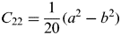 $$C_{22} = \displaystyle{1 \over {20}}(a^2 - b^2 )$$
γ and λ are latitude and longitude of the spacecraft in the Hill reference frame which are given as
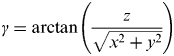 $$\gamma = \arctan \left( {\displaystyle{z \over {\sqrt {x^2 + y^2}}}} \right)$$
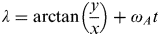 $$\lambda = \arctan \left( {\displaystyle{y \over x}} \right) + \omega _A t$$
where δ r=[x, y, z]T is the position vector of the spacecraft with respect to the asteroid, ω A is the asteroid rotating angular velocity around the Z-axis. Note that the gravity field is time-varying and correlates to the shape and the rotational state of the asteroids.
The dynamic model of the spacecraft-asteroid formation is established in the Hill's reference frame. The effects of gravitational forces from the Sun and the asteroid are taken into consideration in the dynamic equations. Moreover, solar pressure is also included in the dynamic model. Besides, the rotation of the inhomogeneous gravity field of the asteroid is modelled and included in the description of the motion of the formation as shown below (Vasile and Maddock, Reference Vasile and Maddock2012)
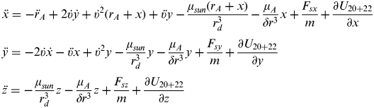 $$\eqalign{ & \ddot x = - \ddot r_A + 2\dot \upsilon \dot y + \dot \upsilon ^2 (r_A + x) + \ddot \upsilon y - \displaystyle{{\mu _{sun} (r_A + x)} \over {r_d^3}} - \displaystyle{{\mu _A} \over {\delta r^3}} x + \displaystyle{{F_{sx}} \over m} + \displaystyle{{\partial U_{20 + 22}} \over {\partial x}} \cr & \ddot y = - 2\dot \upsilon \dot x - \ddot \upsilon x + \dot \upsilon ^2 y - \displaystyle{{\mu _{sun}} \over {r_d^3}} y - \displaystyle{{\mu _A} \over {\delta r^3}} y + \displaystyle{{F_{sy}} \over m} + \displaystyle{{\partial U_{20 + 22}} \over {\partial y}} \cr & \ddot z = - \displaystyle{{\mu _{sun}} \over {r_d^3}} z - \displaystyle{{\mu _A} \over {\delta r^3}} z + \displaystyle{{F_{sz}} \over m} + \displaystyle{{\partial U_{20 + 22}} \over {\partial z}}} $$
with
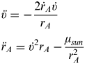 $$\eqalign{ & \ddot \upsilon = - \displaystyle{{2\dot r_A \dot \upsilon} \over {r_A}} \cr & \ddot r_A = \dot \upsilon ^2 r_A - \displaystyle{{\mu _{sun}} \over {r_A^2}}} $$
where μ Sun is the Sun gravity constant, r A and r d are the current orbit radius of the asteroid and spacecraft in the Sun inertial frame, respectively, υ is the asteroid true anomaly,  $\dot \upsilon $ and
 $\ddot \upsilon $ are true anomaly velocity and acceleration, respectively,
 $\dot r_A $ and
 $\ddot r_A $ are the asteroid orbit radius velocity and acceleration, respectively, m is the mass of the spacecraft.
The position vector of the asteroid in the Sun inertial frame is given as
 $${\bf r}_A = [r_A, {\kern 1pt} 0,{\kern 1pt} 0]^T $$
The relative orbit position vector of the spacecraft with respect to the asteroid δ r is expressed in O a-XYZ frame components with unit vector (e x, ey, ez) as
 $$\delta {\bf r}(x,{\kern 1pt} y,{\kern 1pt} z) = x{\bf e}_x + y{\bf e}_y + z{\bf e}_z $$
The spacecraft position vector rd can be described in O a-XYZ frame
 $${\bf r}_d = {\bf r}_A + \delta {\bf r} = (r_A + x){\bf e}_x + y{\bf e}_y + z{\bf e}_z $$
with
 $$r_d = \sqrt {(r_A + x)^2 + y^2 + z^2} $$
(F sx, Fsy, Fsz)T is the solar pressure acting on the surface of the spacecraft which is computed as (Vasile, Reference Vasile2009)
 $$F_s = \eta AP({\bf r}_d /r_d )$$
with P=P 0(r 1AU/r d)2, where η is the reflectivity coefficient, A is the surface area of the spacecraft, P is the solar pressure at the distance r d from the Sun, r 1AU is one astronomical unit, the solar pressure at 1 AU is P0=4·563×10−6N/m 2.
2.2. Lyapunov Control Law
Control force in the opposite direction of the resultant of all the perturbations including the solar pressure, the gravity of the Sun and the asteroid and the gravity field of the asteroid is required to compensate the orbit deviations. The centrifugal and Coriolis forces acting on the spacecraft are negligible. Any other non-spherical terms in the gravity field expansion result in only a second order additional perturbation. A simple control law based on the Lyapunov control function is derived as (Vasile and Maddock, Reference Vasile and Maddock2012):
 $$V = \displaystyle{1 \over 2}\delta v^2 + \displaystyle{1 \over 2}K((x - x_{ref} )^2 + (y - y_{ref} )^2 + (z - z_{ref} )^2 )$$
where δ rref=[x ref, yref, zref]T and δ r=[x, y, z]T are the coordinates of spacecraft along the nominal and true formation orbit with respect to the asteroid, respectively, δ v is the true velocity vector of the spacecraft.
To maintain the spacecraft orbits close to the nominal one, a control input u is required to satisfy the condition that dV/dt<0. A possible control is given by
 $${\bf u} = - \left( { - \displaystyle{{\mu _A} \over {\delta r^3}} \delta {\bf r} + \displaystyle{{F_s} \over m}} \right) - K(\delta {\bf r} - \delta {\bf r}_{ref} ) - c_d \delta {\bf v}$$
where K and c d are the elastic and dissipative coefficients, respectively. Note that the true orbits of the spacecraft are never known exactly, thus the estimated states are introduced into the full dynamics model in Equation (7). Then the control law is written as (Vetrisano et al., Reference Vetrisano, Yang and Vasile2012)
 $${\bf u} = - \left( { - \displaystyle{{\mu _A} \over {\delta r^3}} \delta {\bf r}_{est} + \displaystyle{{F_s} \over m}} \right) - K(\delta {\bf r}_{est} - \delta {\bf r}_{ref} ) - c_d \delta {\bf \dot v}_{est} $$
where δ rest and  $\delta {\bf \dot v}_{est} $ are the estimated position and velocity of the spacecraft.
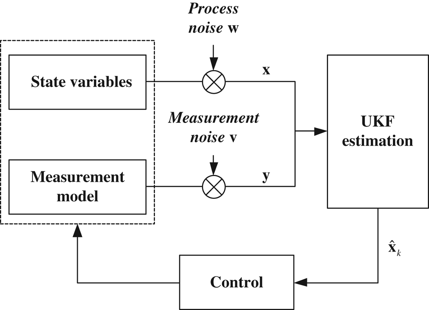
Once the controller is inserted in the spacecraft dynamics, one obtains a closed loop problem in which control is performed together with estimation, and the filter equation has to consider the action of the controller itself (see Figure 2). During the controlled phases, it is assumed that the asteroid trajectory is known, so the only state variables to be estimated are those relating to the spacecraft formation.
Navigation and control system.
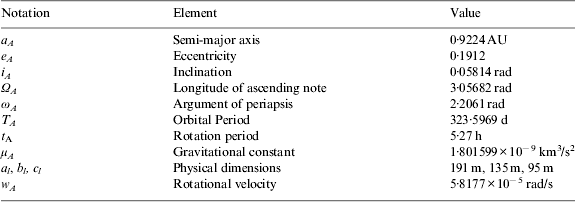
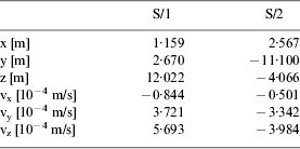
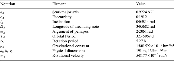
The present work takes 99942 Apophis as the central body of the formation as it is particularly interesting due to its high impact probability and a logical choice for a deflection mission. The spacecraft formation is assumed to fly in the proximity of Apophis at a distance of about 1 km. The Keplerian elements along with the physical properties of Apophis are listed in Table 1 (Vetrisano et al., Reference Vetrisano, Yang and Vasile2012). The orbits of the two spacecraft are given in terms of Cartesian coordinate variation with respect to the asteroid, as reported in Table 2, with the two spacecraft numbered 1 and 2, respectively. These orbits were designed to maintain the spacecraft close to the asteroid and reduce the requirements for control.
Orbital and physical properties of 99942 Apophis.
Initial spacecraft orbit parameters.

Figure 3 shows the orbits of the two spacecraft flying in the formation under the perturbations and control force with respect to 99942 Apophis for 300 days in Hill's reference frame. The controller, K is set as 10−5/s2 while the steady dissipative coefficient c d is set as 10−4/s. During the analysis, an initial mass of spacecraft is 265 kg with the maximum cross section area of about 20 m2. A mean value of 0·2 for the reflectivity coefficient is assumed. In general, an uncertainty of 20% solar pressure is introduced as random noise.
Relative orbits of the spacecraft formation.
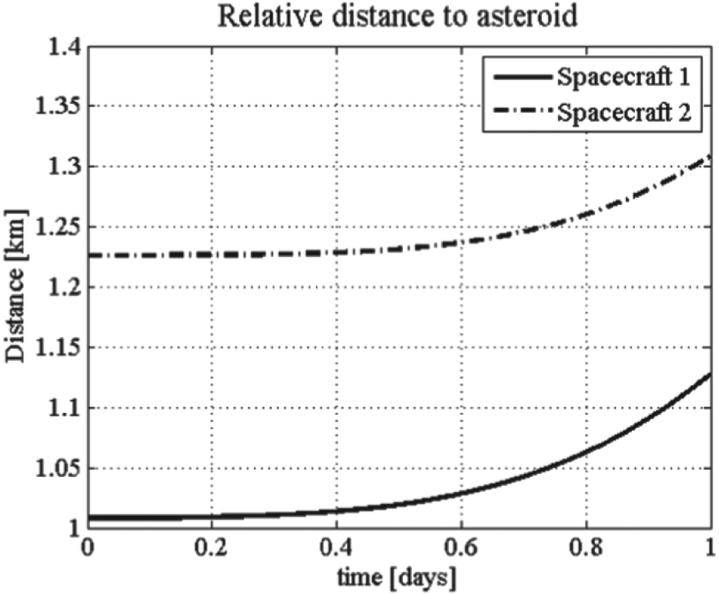
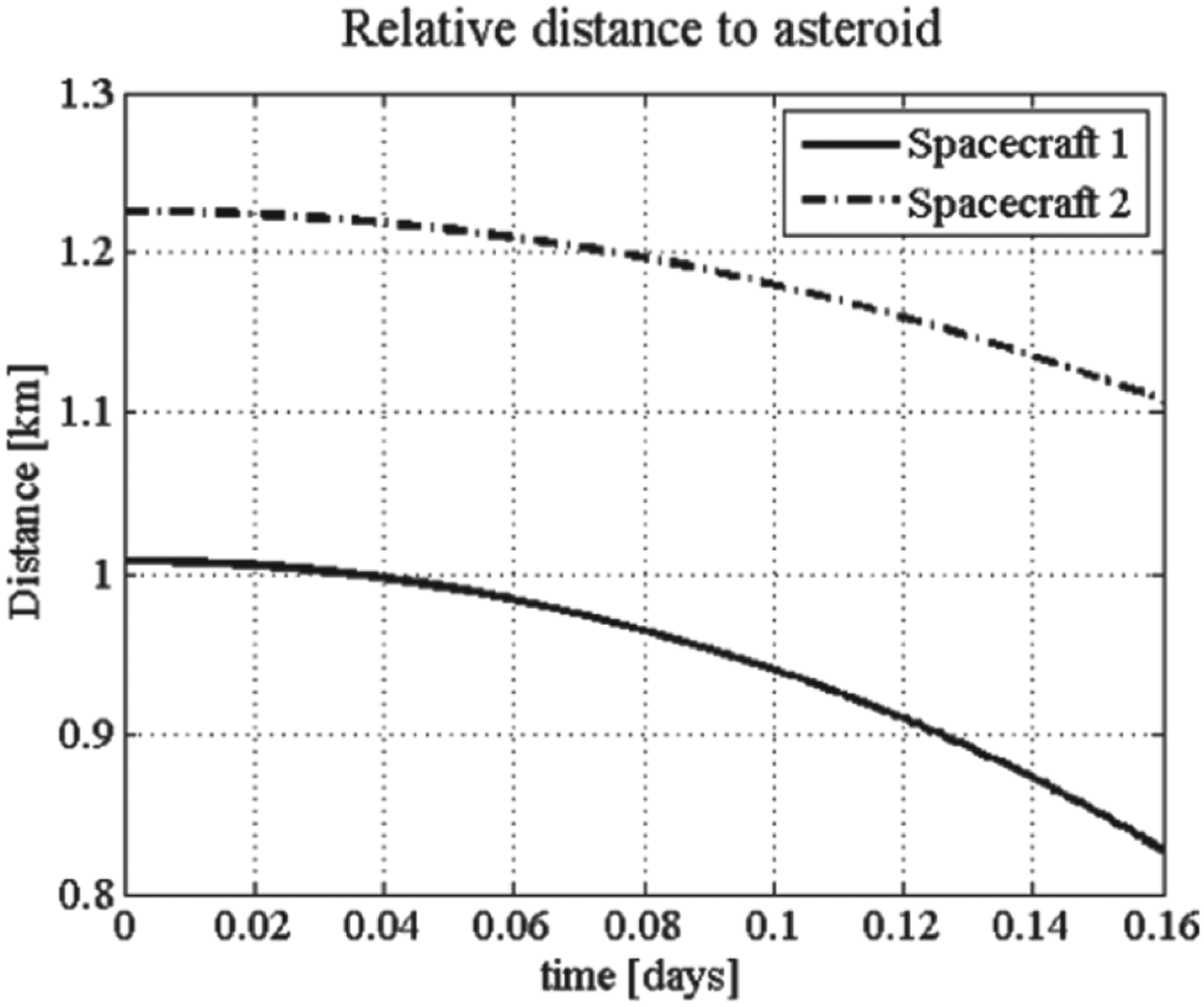
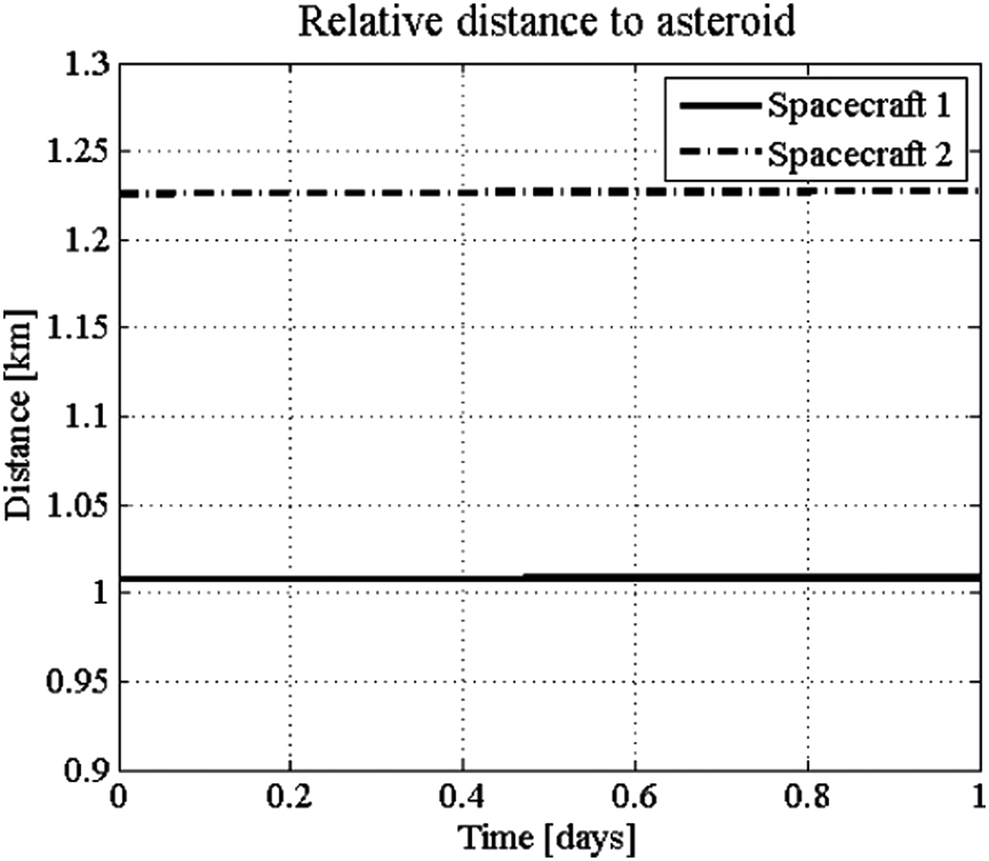
Given by Equation (7), the resultant of all the external forces acting on the spacecraft is not zero. The effect of the perturbations of the Sun gravity force and solar radiation pressure is that the spacecraft will diverge from a close proximity trajectory (see Figure 4(a)). All the perturbations introduced in Equation (7) make the spacecraft crash on the asteroid (see Figure 4(b)).
Relative distance under Sun gravity force and solar radiation pressure.
Relative distance under all perturbations.
An example of the combined filter process and the controller is reported in Figure 5. The simulation period is set to one day. Simulation results show that this control law is effective in keeping the spacecraft orbit stable under the effect of perturbations.
Relative distance under all perturbations and control forces.
3. NAVIGATION SENSOR MODELLING
The accurate measurement model plays a key role in the orbit determination problem. A novel measurement model is established based on the most common use of the optical camera coupled with LIDAR which is used to measure the range from the spacecraft to the asteroid surface while cameras, in conjunction with attitude sensors, are used to get a fix on the asteroid and triangulate the relative position of the spacecraft. The spacecraft-to-asteroid measurement models are defined in Section 3.1 and 3.2, the inter-spacecraft measurement models are defined in Section 3.3.
3.1. CCD Measurement Model
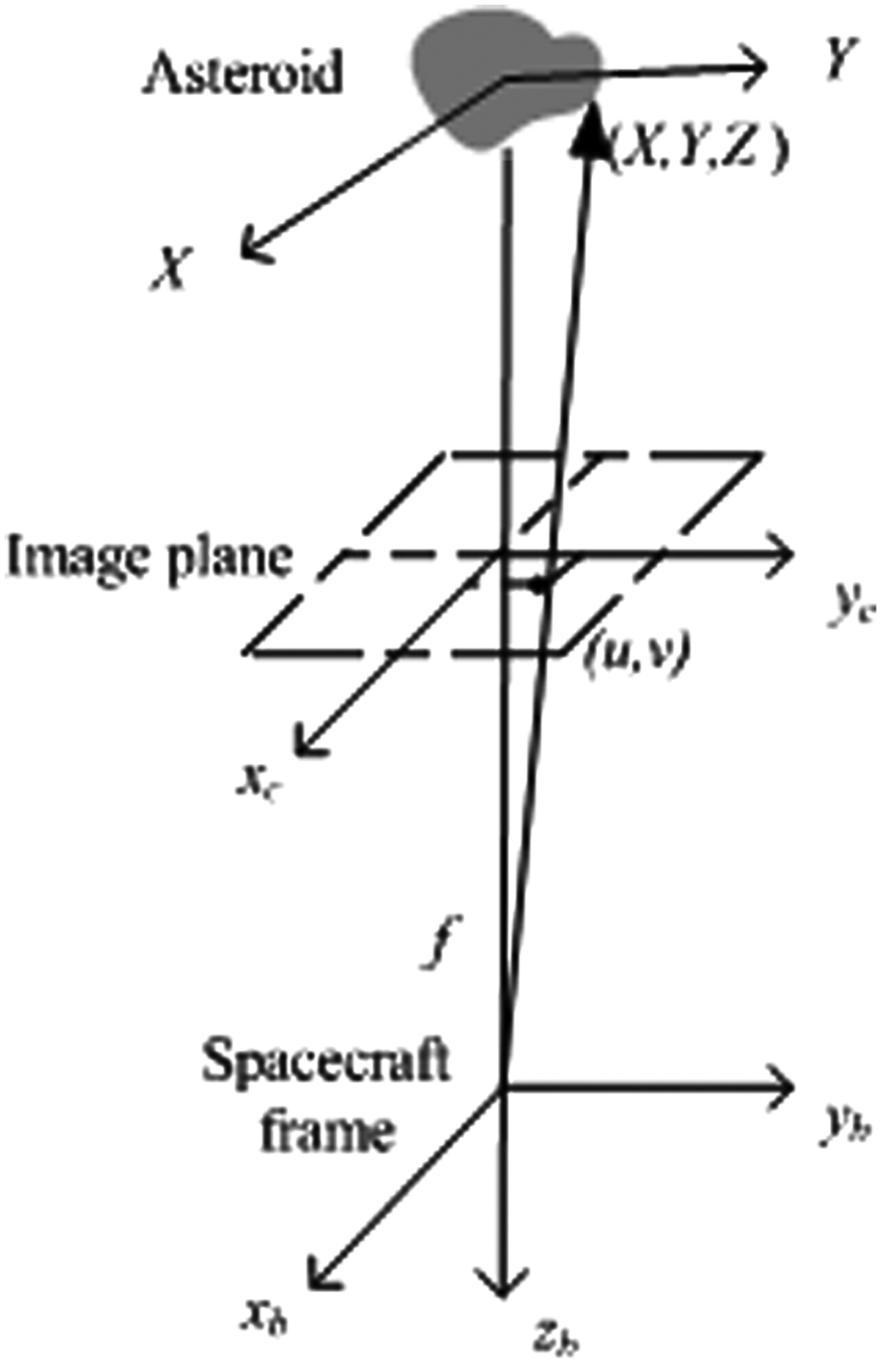
A CCD camera provides the direct observation of points on the surface of the asteroid. In this paper, the image plane is in front of the centre of perspective projection (see Figure 6). It is assumed that, from a pre-characterisation phase, the position of the surface point is available which is randomly picked up on the asteroid surface as shown in Equation (1). The observation can be constructed in unit vector form as
 $$\displaystyle{{[u\;{\rm v}\;f]^T} \over {\sqrt {u^2 + {\rm v}^2 + f^2}}} = T_a^c \displaystyle{{[X - x\;\;Y - y\;\;Z - z]^T} \over {\sqrt {(X - x)^2 + (Y - y)^2 + (Z - z)^2}}} $$
where the left hand side is the line-of-sight unit vector from camera to the random point expressed in the camera frame, [u, v]T are the coordinates of the ith surface point in the image plane, f is focal length, [X Y Z]T is the location of the point with respect to the centre of the asteroid. T ac is the transformation matrix which transforms the position vector from Hill's reference frame to camera frame which is given as
$$\eqalign{{\bf T}_a^c = & \left[ {\matrix{ 1 & 0 & 0 \cr 0 & {\cos \phi} & {\sin \phi} \cr 0 & { - \sin \phi} & {\cos \phi} \cr}} \right]\left[ {\matrix{ {\cos \theta} & 0 & { - \sin \theta} \cr 0 & 1 & 0 \cr {\sin \theta} & 0 & {\cos \theta} \cr}} \right]\left[ {\matrix{ {\cos \psi} & {\sin \psi} & 0 \cr { - \sin \psi} & {\cos \psi} & 0 \cr 0 & 0 & 1 \cr}} \right] \cr\noalign{\cr} & = \left[ {\matrix{ {\cos \theta \cos \psi} & {\cos \theta \sin \psi} & { - \sin \theta} \cr {\sin \phi \sin \theta \cos \psi - \cos \phi \sin \psi} & {\sin \phi \sin \theta \sin \psi + \cos \phi \cos \psi} & {\sin \phi \cos \theta} \cr {\cos \phi \sin \theta \cos \psi + \sin \phi \sin \psi} & {\cos \phi \sin \theta \sin \psi - \sin \phi \cos \psi} & {\cos \phi \cos \theta} \cr}} \right]} $$with ϕ, θ, ψ, are the attitude angles considered to be already known.
Camera imaging geometry.
The pixel point [u i, vi]T (i=1, 2) measured by spacecraft i which is given by the following relations:
 $$\eqalign{& { u}_i = f\displaystyle{{x_{c,i}} \over {z_{c,i}}} \cr & {\rm v}_i = f\displaystyle{{y_{c,i}} \over {z_{c,i}}}} $$
where [x c,i, yc,i, zc,i]T are the components of the imaging point measured by camera mounted on the spacecraft i.
Therefore, the measurement model of the CCD camera is presented as
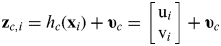 $${\bf z}_{c,i} = h_c ({\bf x}_i ) + {\bf \upsilon} _c = \left[ {\matrix{ {{\rm u}_i} \cr {{\rm v}_i} \cr}} \right] + {\bf \upsilon} _c $$
where zc,i is the measurement vector of the camera mounted on spacecraft i, h c(xi) refers to a function relating the states to the measurements, xi is the state variables of the spacecraft i, υc is the measurement noise which can be assumed as the zero-mean Gaussian white noise.
3.2. LIDAR Measurement Model
LIDAR is a pulse laser that measures the travelling time of the pulse between the spacecraft and the asteroid. A range measurement combined with the camera image of one visible surface point was proved enough for the navigation system to be observable (Dionne, Reference Dionne2009). This assumes that the imaging point is the same as the point illuminated by LIDAR. The range between the spacecraft to the illuminated point is
 $$d_i = \sqrt {x_{c,i}^2 + y_{c,i}^2 + z_{c,i}^2} $$
Thus, the LIDAR range measurement model with measurement noise is shown below:
 $$z_{L,i} = h_L \,({\bf x}_i ) + \upsilon _L = [d_i ] + \upsilon _L $$
where z L,i is the measurement LIDAR mounted on spacecraft i, υ L is the LIDAR measurement noise which is modelled as white noise. The measured range d i can also be pre-processed in combination with the related camera provided angles α i, δi. The observation model is shown in Figure 7. The azimuth angle α i and elevation angle δ i can be written as
 $$\eqalign{& \alpha _i = \arctan \displaystyle{{y_{c,i}} \over {x_{c,i}}} \cr & \delta _i = \arctan \displaystyle{{z_{c,i}} \over {\sqrt {x_{c,i}^2 + y_{c,i}^2}}}} $$
3-dimension measurements.
As a consequence, the update module takes [d i, αi, δi]T as inputs. The measurement equation is given as
 $${\bf z}_{c,L,i} = h_{c,L} ({\bf x}_i ) + {\bf \upsilon} _{c,L,i} = [\matrix{ {d_i,} & {\alpha _i,} & {\delta _i} \cr} ]^T + {\bf \upsilon} _{c,L,i} $$
where zc,L,i is the measurement vector of the camera information aided by the range measurement coming from spacecraft i, υc,L,i is the measurement noise including the range and angular measurement noises.
3.3. Inter-spacecraft Measurement Model
The inter-spacecraft links are considered to add into the measurement model. This assumes that the relative range between the two spacecraft is small so that inter-spacecraft relative position measurement can be observed. Meanwhile, the spacecraft are suitable for reflecting the sensor signal. The relative position vector from one spacecraft to the other is described in the Hill's reference frame as
 $${\bf r}_2 - {\bf r}_1 = [\matrix{ {x_2 - x_1} & {y_2 - y_1} & {z_2 - z_1} \cr} ]^T $$
Transform this vector to the spacecraft body frame (the spacecraft body frame is coincident with the camera frame), and then the relative position vector from spacecraft one to two is given as:
 $${\bf r}_{12} = [x_{12} \;y_{12} \;z_{12} ]^T = {\bf T}_a^c [\matrix{ {x_2 - x_1} & {y_2 - y_1} & {z_2 - z_1} \cr} ]^T $$
The inter-spacecraft range measured by the LIDAR mounted on spacecraft one is
 $$d_{12} = \left\| {{\bf r}_{12}} \right\|$$
When measurement noise is taken into account, the inter-range measurement model can be written as:
 $${\bf z}_{12} = h_{12} ({\bf x}_1 ) + {\bf \upsilon} _{12} = [d_{12} ] + {\bf \upsilon} _{12} $$
where z12 denotes the inter-spacecraft range measurement vector from spacecraft one to two, x is the state variables of both spacecraft. Without loss of generality, the inter-range measurement noise υ 12 is modelled as a zero mean white noise based on the characteristic of the instrument itself. Note that the camera can also provide the inter-angles (α 12, δ 12) and the formulation can be derived as
 $$\eqalign{& \alpha _{12} = \arctan \displaystyle{{y_{12}} \over {x_{12}}} \cr & \delta _{12} = \arctan \displaystyle{{z_{12}} \over {\sqrt {x_{12}^2 + y_{12}^2}}}} $$
As a consequence, the update module takes [d 12, α 12, δ 12]T as inputs. The measurement model is
 $${\bf z}_{rel,12} = h_{rel,12} ({\bf x}_1 ) + {\bf \upsilon} _{rel,12} = [\matrix{ {d_{12}} & {\alpha _{12}} & {\delta _{12}} \cr} ]^T + {\bf \upsilon} _{rel,12} $$
where zrel,12 refers to the 3-dimention position measurement vector, υrel,12 is the measurement noise which includes the inter-range and inter-angular measurement noises.
4. ORBIT DETERMINATION ALGORITHM
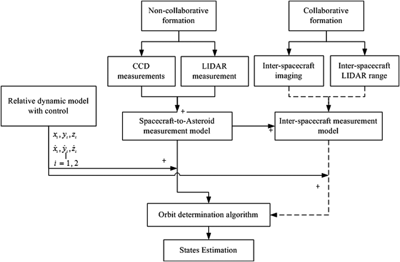
This section describes the orbit determination architecture (see Figure 8) by presenting the state equations and four measurement scenarios, in Sections 4.1 and 4.2, respectively. The UKF algorithm is introduced in Section 4.3.
Orbit determination architecture.
4.1. State Equations
Simultaneously estimating all spacecraft in the formation produced identical relative results to those obtained by independently estimating each of the spacecraft (Kelbel et al., Reference Kelbel, Lee, Long, Carpenter and Gramling2001). To this end, 12 states (three position and three velocity state variables for each spacecraft) are estimated in the same filter. The state vectors are given by
 $${\bf x} = [\matrix{ {x_1} & {y_1} & {z_1} & {\dot x_1} & {\dot y_1} & {\dot z_1} & {x_2} & {y_2} & {z_2} & {\dot x_2} & {\dot y_2} & {\dot z_2} \cr} ]^T $$
where [x i, yi, zi]T and 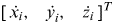 $[\matrix{ {\dot x_i,} & {\dot y_i,} & {\dot z_i} \cr} ]^T $, i=1, 2 are the coordinates of the position and velocity of the ith spacecraft relative to the asteroid.
The state equation is
 $${\bf \dot x} = f\,({\bf x}) + {\bf w}$$
with
 $$f\,({\bf x}) = [\matrix{ {\dot x_1} & {\dot y_1} & {\dot z_1} & {\ddot x_1} & {\ddot y_1} & {\ddot z_1} & {\dot x_2} & {\dot y_2} & {\dot z_2} & {\ddot x_2} & {\ddot y_2} & {\ddot z_2} \cr} ]^T $$
where w is the process noise in the order of 10−12, 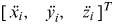 $[\matrix{ {\ddot x_i,} & {\ddot y_i,} & {\ddot z_i} \cr} ]^T $ (i=1, 2) are the acceleration of the spacecraft 1 and 2, respectively, which are given in Equation (7).
4.2. Measurement Scenarios
It is assumed that the spacecraft-to-asteroid measurements and inter-spacecraft communication are transmitted and received at the same time. Four measurement scenarios are introduced based on the different combinations of the multiple measurements. Firstly, Scenario 1 is the basic measurement model that only contains the spacecraft-to-asteroid image information and range measurement. Secondly, angular measurements are added to the measurement model to form Scenario 2. Clearly, Scenarios 1 and 2 are the non-collaborative scenarios. In contrast, Scenarios 3 and 4 are collaborative. The inter-spacecraft range measurements are taken into account in Scenario 3 whereas Scenario 4 considers both the inter-range and inter-angular measurements.
The purpose of presenting the four scenarios is to firstly demonstrate the effect of increasing the number of the measurements on the filter performance and analyse the sensitivity of different types of the measurements to the orbit determination accuracy. The other purpose is to quantify the advantages of combining the spacecraft-to-asteroid measurements with the inter-spacecraft communication.
4.2.1. Non-collaborative Scenario 1
In Scenario 1, the camera and LIDAR range measurements of the spacecraft with respect to the asteroid are taken in the measurement model which is given as
 $${\bf z}_1 = h_1 ({\bf x}) + {\bf \upsilon} _1 = \left[ {\matrix{ {h_c ({\bf x}_1 )} \cr {h_L ({\bf x}_1 )} \cr {h_c ({\bf x}_2 )} \cr {h_L ({\bf x}_2 )} \cr}} \right] + \left[ {\matrix{ {{\bf \upsilon} _{c,1}} \cr {{\bf \upsilon} _{L,1}} \cr {{\bf \upsilon} _{c,2}} \cr {{\bf \upsilon} _{L,2}} \cr}} \right]$$
where z1 is the measurement vector, υ1 is the integrated measurement noise coming from camera and LIDAR with covariance R1.
4.2.2 Non-collaborative Scenario 2
In Scenario 2, the angular measurements [φ i, θi] (i=1, 2) are added into the measurement model of Scenario 1. The LIDAR range measurement with the commanded angles composes a 3-dimension position vector of the spacecraft with respect to the asteroid. The measurement equation of Scenario 2 is given as
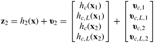 $${\bf z}_2 = h_2 ({\bf x}) + {\bf \upsilon} _2 = \left[ {\matrix{ {h_c ({\bf x}_1 )} \cr {h_{c,L} ({\bf x}_1 )} \cr {h_c ({\bf x}_2 )} \cr {h_{c,L} ({\bf x}_2 )} \cr}} \right] + \left[ {\matrix{ {{\bf \upsilon} _{c,1}} \cr {{\bf \upsilon} _{c,L,1}} \cr {{\bf \upsilon} _{c,2}} \cr {{\bf \upsilon} _{c,L,2}} \cr}} \right]$$
where z2 is the measurement vector containing the camera information and 3-dimension position vector consisting of the angular measurements and LIDAR range, υ2 is the noise including the camera image, angular and range measurements with covariance matrix R2.
4.2.3. Collaborative Scenario 3
In Scenario 3, the measurements for the relative motion estimator are composed of CCD image, LIDAR range measurements with respect to the asteroid and two-way inter-range measurements. The measurement model is given by
 $${\bf z}_3 = h_3 ({\bf x}) + {\bf \upsilon} _3 = \left[ {\matrix{ {h_c ({\bf x}_1 )} \cr {h_{c,L} ({\bf x}_1 )} \cr {h_{12} ({\bf x}_1 )} \cr {h_c ({\bf x}_2 )} \cr {h_{c,L} ({\bf x}_2 )} \cr {h_{21} ({\bf x}_2 )} \cr}} \right] + \left[ {\matrix{ {{\bf \upsilon} _{c,1}} \cr {{\bf \upsilon} _{c,L,1}} \cr {{\bf \upsilon} _{12}} \cr {{\bf \upsilon} _{c,2}} \cr {{\bf \upsilon} _{c,L,2}} \cr {{\bf \upsilon} _{21}} \cr}} \right]$$
where z3 is the measurement vector, υ3 is the measurement noise including the spacecraft-to-asteroid measurement noise as well as the two-way inter-range measurement noise, with covariance matrix R3.
4.2.4 Collaborative Scenario 4
In this scenario, the inter-spacecraft measurements not only include the relative range measurement, but also the angular information. These inter-spacecraft measurements construct the 3-dimension position vector from one spacecraft to the other. The measurement vector in Scenario 4 can be written as
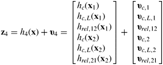 $${\bf z}_4 = h_4 ({\bf x}) + {\bf \upsilon} _4 = \left[ {\matrix{ {h_c ({\bf x}_1 )} \cr {h_{c,L} ({\bf x}_1 )} \cr {h_{rel,12} ({\bf x}_1 )} \cr {h_c ({\bf x}_2 )} \cr {h_{c,L} ({\bf x}_2 )} \cr {h_{rel,21} ({\bf x}_2 )} \cr}} \right] + \left[ {\matrix{ {{\bf \upsilon} _{c,1}} \cr {{\bf \upsilon} _{c,L,1}} \cr {{\bf \upsilon} _{rel,12}} \cr {{\bf \upsilon} _{c,2}} \cr {{\bf \upsilon} _{c,L,2}} \cr {{\bf \upsilon} _{rel,21}} \cr}} \right]$$
where z4 is the measurement vector, υ4 is a measurement noise including the spacecraft-to-asteroid measurement noise as well as the inter-spacecraft position measurement noise, with covariance matrix R4.
4.3. UKF Algorithm
According to the nonlinear equations of motion and measurement, the UKF is used to enhance the orbit determination accuracy for the four scenarios. Moreover, it can better reduce the impact of the multiple measurement noise. The general nonlinear discrete-time process model and discrete-time measurement model in a state-space form at step k+1 are given by
 $${\bf x}_{k + 1} = f\,({\bf x}_k, \;{\bf u}_k, \;k) + {\bf w}_k, \quad {\bf w}_k \sim N(0,{\bf Q}_k )$$
 $${\bf z}_k = h({\bf x}_k, \;{\bf u}_k, \;k) + {\bf \upsilon} _k, \quad {\bf \upsilon} _k \sim N(0,{\bf R}_k )$$
where uk is the control input, wk is the process noise with the covariance Qk, υk is the measurement noise with the covariance Rk.
The initial conditions at t 0 are assumed to be known and have the following form
 $${\bf \hat x}_0 = E({\bf x}_0 )$$
 $${\bf P}_0 = E[({\bf x}_0 - {\bf \hat x}_0 )({\bf x}_0 - {\bf \hat x}_0 )^T ]$$
The 2n+1 sigma points χ i are propagated through the nonlinear dynamics and recombined to generate a propagated mean and covariance (Guo et al., Reference Guo, Cai and Hu2013)
 $${\bf \chi} _{k|k}^i = \left[ {{\hskip3 \bar{\hskip-3\bf \chi}} _{k|k}^i \quad { \bar{\hskip-3\bf \chi}} _{k|k}^i + \left( {\sqrt {(n + \lambda ){\bf P}_{k|k} + {\bf Q}_k}} \right)_i \quad { \bar {\hskip-3\bf\chi}} _{k|k}^i - \left( {\sqrt {(n + \lambda ){\bf P}_{k|k} + {\bf Q}_k}} \right)_i} \right]$$
with
 $$\lambda = \alpha ^2 (n + \kappa ) - n$$
is a scaling parameter, where n is size of the state variables. Constant α and κ determine the extension of these vectors around  ${\bf \bar x}$ and usually set to be 1e−4⩽α⩽1.
Weighted sample mean and covariance W i(m) and W i(c) are given as
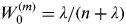 $$W_0 ^{(m)} = \lambda /(n + \lambda )$$
 $$W_0^{(c)} = \lambda /(n + \lambda ) + (1 - \alpha ^2 + \beta )$$
 $$W_i^{(m)} = W_i^{(c)} = \lambda /[2(n + \lambda )],\quad i = 1,\;2, \ldots, \;2n$$
where the good starting guess for parameter β is 2.
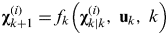
The transformed set of sigma points are evaluated for each of the points by
 $${\bf \chi} _{k + 1}^{(i)} = f_k \left( {{\bf \chi} _{k|k}^{(i)}, \;{\bf u}_k, \;k} \right)$$
The predicted mean and covariance for the state estimate is calculated using a weighted sum of the points
 $${\bf \hat x}_{k + 1|k} = \sum\limits_{i = 0}^{2n} {W_i^{(m)} {\bf \chi} _{k + 1}^{(i)}} $$
 $${\bf P}_{k + 1|k} = \sum\limits_{i = 0}^{2n} {W_i^{(c)} \left( {{\bf \chi} _{k + 1}^{(i)} - {\bf \hat x}_{k + 1|k}} \right)} \left( {{\bf \chi} _{k + 1}^{(i)} - {\bf \hat x}_{k + 1|k}} \right)^T + {\bf Q}_K $$
The mean observation is given by
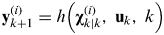 $${\bf y}_{k + 1}^{(i)} = h\left( {{\bf \chi} _{k|k}^{(i)}, \;{\bf u}_k, \;k} \right)$$
 $${\bf \hat y}_{k + 1|k} = \sum\limits_{i = 0}^{2n} {W_i^{(m)} {\bf y}_{k + 1}^{(i)}} $$
The updated covariance is given by
 $${\bf P}_{y,k + 1} = \sum\limits_{i = 0}^{2n} {W_i^{(c)} \left( {{\bf y}_{k + 1}^{(i)} - {\bf \hat y}_{k + 1|k}} \right)\left( {{\bf y}_{k + 1}^{(i)} - {\bf \hat y}_{k + 1|k}} \right)^T + {\bf R}_k} $$
 $${\bf P}_{xy,k + 1} = \sum\limits_{i = 0}^{2n} {W_i^{(c)} \left( {{\bf \chi} _{k + 1}^{(i)} - {\bf \hat x} _{k + 1|k}} \right)\left( {{\bf y}_{k + 1}^{(i)} - {\bf \hat y}_{k + 1|k}} \right)^T} $$
Finally, the state vector  ${\bf \hat x}_{k + 1|k + 1} $ and covariance updated matrix Pk+1|k+1 are represented as follows
 $${\bf \hat x}_{k + 1} = {\bf \hat x}_{k + 1|k} + {\bf K}_{k + 1} ({\bf y}_{k + 1} - {\bf \hat y}_{k + 1|k} )$$
 $${\bf P}_{k + 1} = {\bf P}_{k + 1|k} - {\bf K}_{k + 1} {\bf P}_{y,\;k + 1} {\bf K}_{k + 1}^T $$
 $${\bf K}_{k + 1} = {\bf P}_{xy,k + 1} {\bf P}_{y,k + 1}^{ - 1} $$
where Kk+1 is the Kalman gain matrix. The state variables  ${\bf \hat x}_{k + 1} $ and
 ${\bf \hat x}_{k + 1|k} $ represent updated and predicted estimates of state at time t k, Pk+1 and Pk+1|k are covariance matrices of their errors, respectively.
5. SIMULATION RESULTS
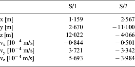
This section presents the simulation results of the four scenarios and evaluates their performances by comparing them. The numerical simulation is implemented under the following conditions. The initial position and velocity of each spacecraft with respect to Apophis are shown in Table 2. The gravitational constant of the Sun is 1·327×1011 km3/s2. The initial position and velocity of the Apophis in the inertial frame are summarized in Table 3.
The initial position of the Apophis in the Sun inertial coordinate system.

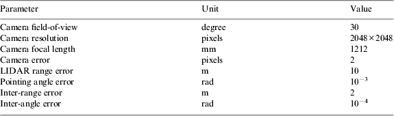
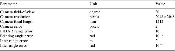
The errors of the measurements which are incorporated into each simulation are summarized in Table 4 (Vetrisano et al., Reference Vetrisano, Yang and Vasile2012). In the present work, no biases are included in the measurement model. Camera imaging error is set to two pixels and the pointing error of angles is 10−3 rad for spacecraft-to-asteroid measurements and 10−4 rad for inter-spacecraft measurements (Vetrisano and Vasile, Reference Vetrisano and Vasile2012). The error of LIDAR is set to 10 m with respect to the asteroid and 2 m with respect to spacecraft (Dionne, Reference Dionne2009).
Sensor characteristics.
The simulation time is one day with a time interval of 30 minutes. The initial error of the position and velocity of each spacecraft is designed to be 10% of the initial value. The process and measurement noise parameters w and v are assumed to be uncorrelated with each other.
The main parameters of the UKF include λ, α, κ and β. α is usually set to be 1e−4⩽α⩽1. κ is usually equal to 3-n, with n is the size of the state variables. Good starting guess for parameter β is set as 2 according to the UKF theory (Crassidis and Junkins, Reference Crassidis and Junkins2011). λ can be calculated by Equation (43). Consequently, α=0·01, β=2, λ=−9. The observation noise covariance matrix R is a square and symmetrical matrix with observation errors as its diagonal terms. The process noise covariance matrix Q is set as
 $${\bf Q} = diag[\matrix{ {10^{ - 24}} & {10^{ - 24}} & \ldots & {10^{ - 24}} \cr} ]_{12 \times 12} $$
The initial covariance matrix P0 is set as
 $${\bf P}_0 = \left[ {\matrix{ {0{\cdot}64 \times 10^4\, {\bf I}_{3 \times 3}} & {} & {} & 0 \cr {} & {0{\cdot}36 \times 10^{ - 6}\, {\bf I}_{3 \times 3}} & {} & {} \cr {} & {} & {0{\cdot}81 \times 10^{ 4}\, {\bf I}_{3 \times 3}} & {} \cr 0 & {} & {} & {0{\cdot}09 \times 10^{ - 6} \,{\bf I}_{3 \times 3}} \cr}} \right]_{12 \times 12} $$
5.1. Scenario 1: Camera and LIDAR range measurements
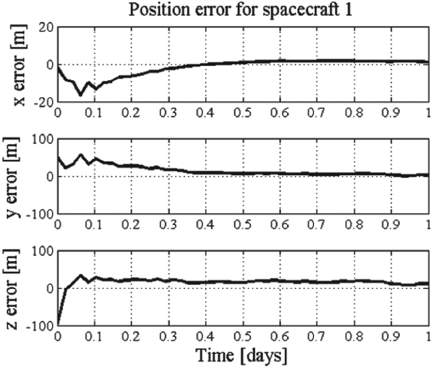
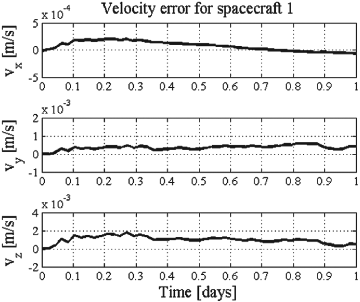
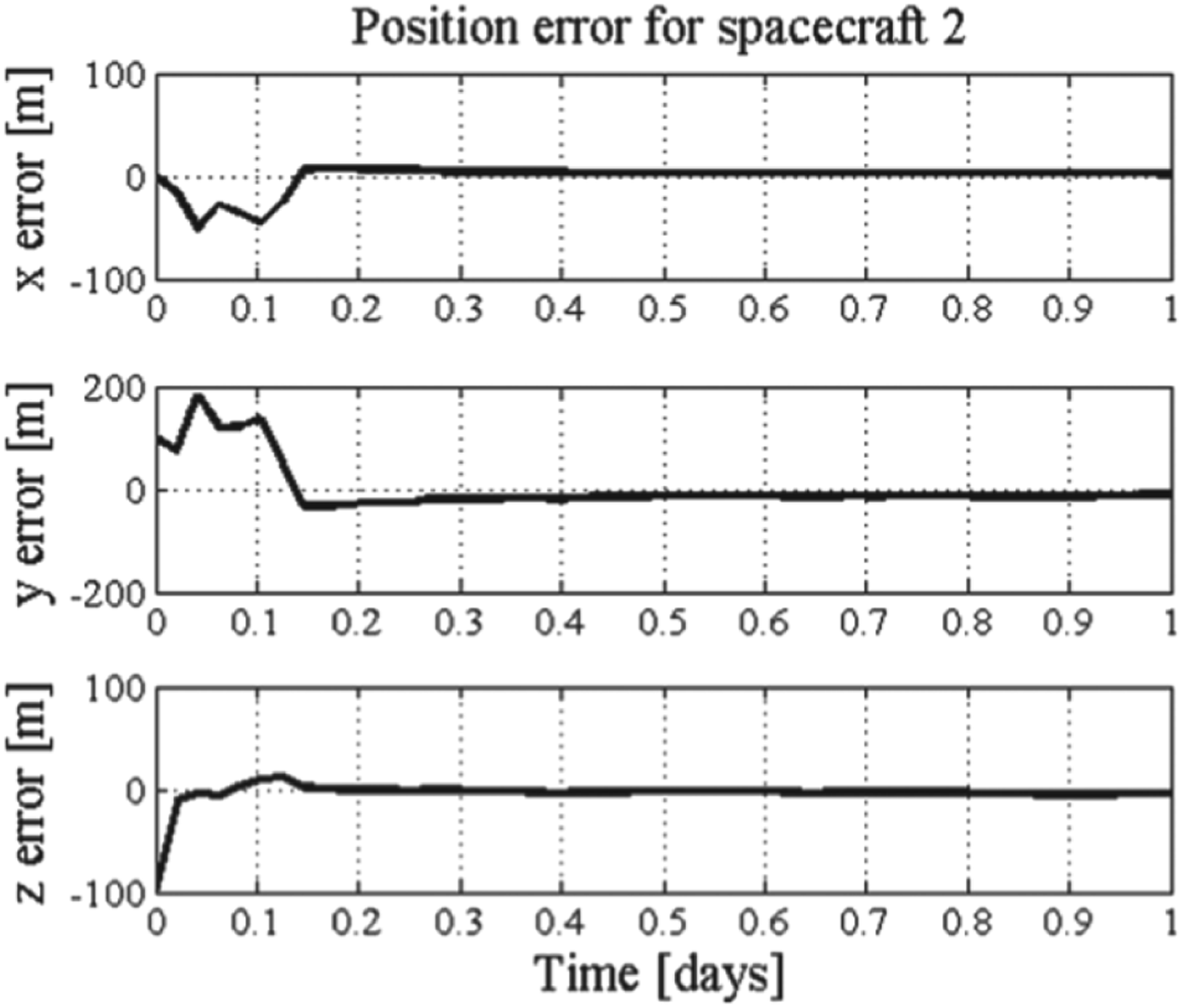
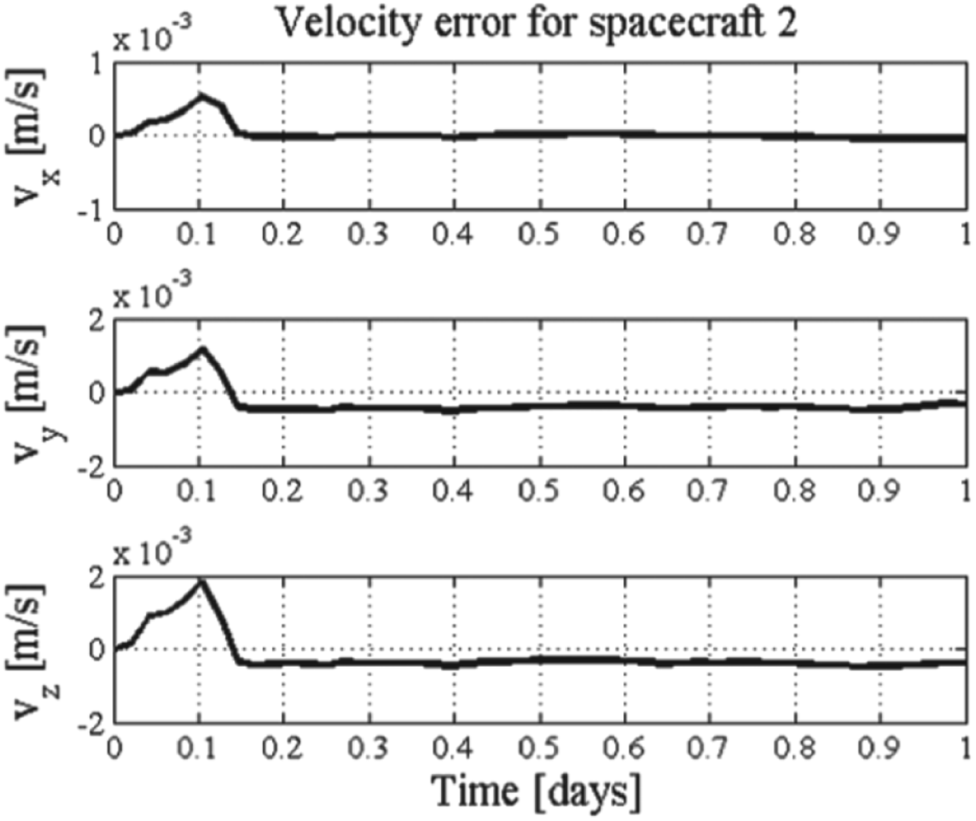
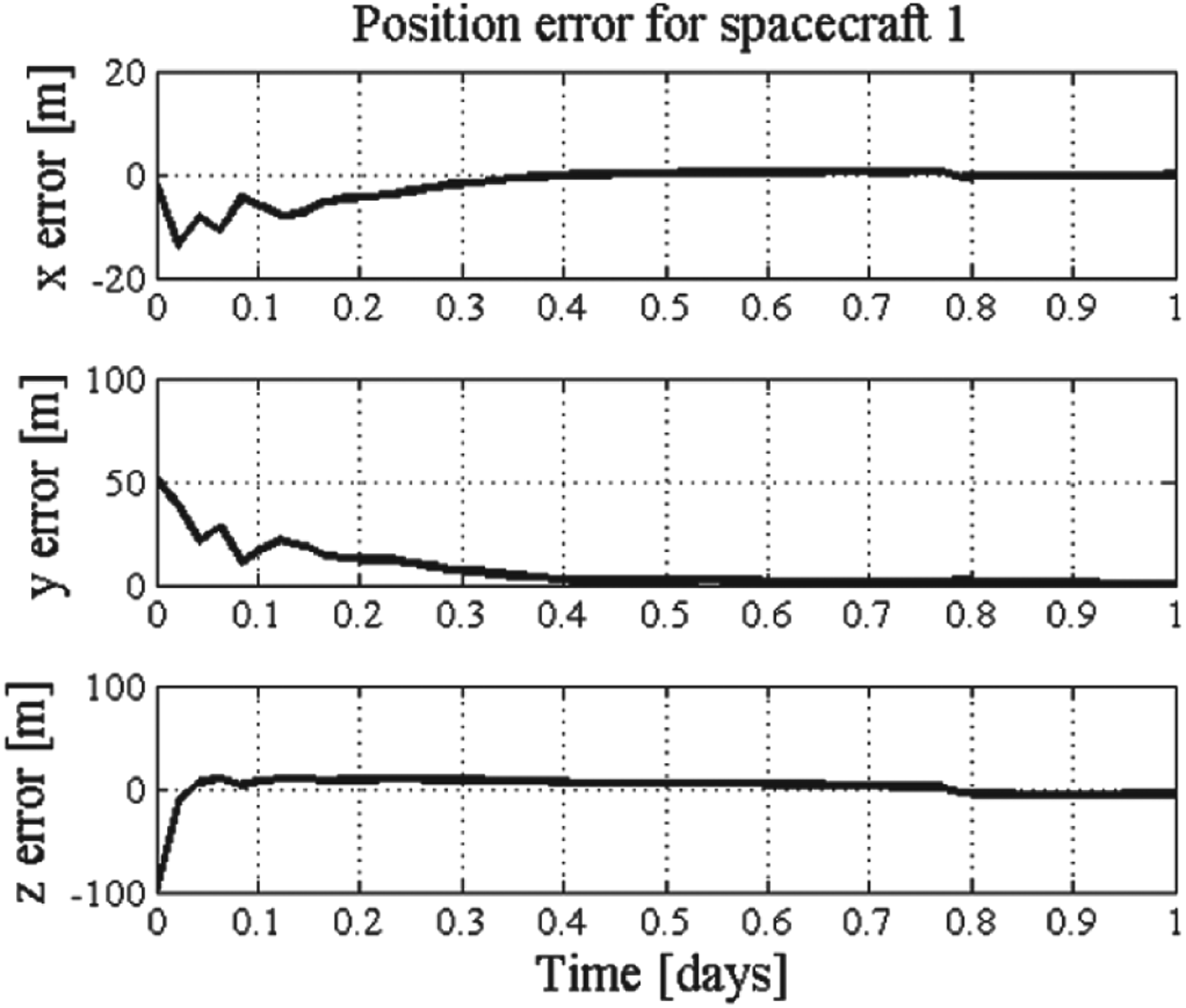
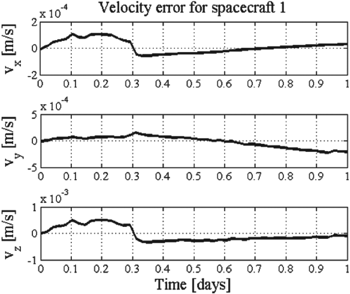
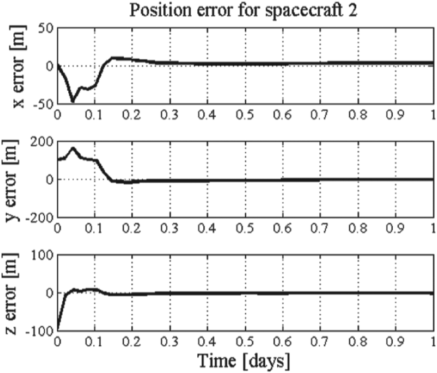
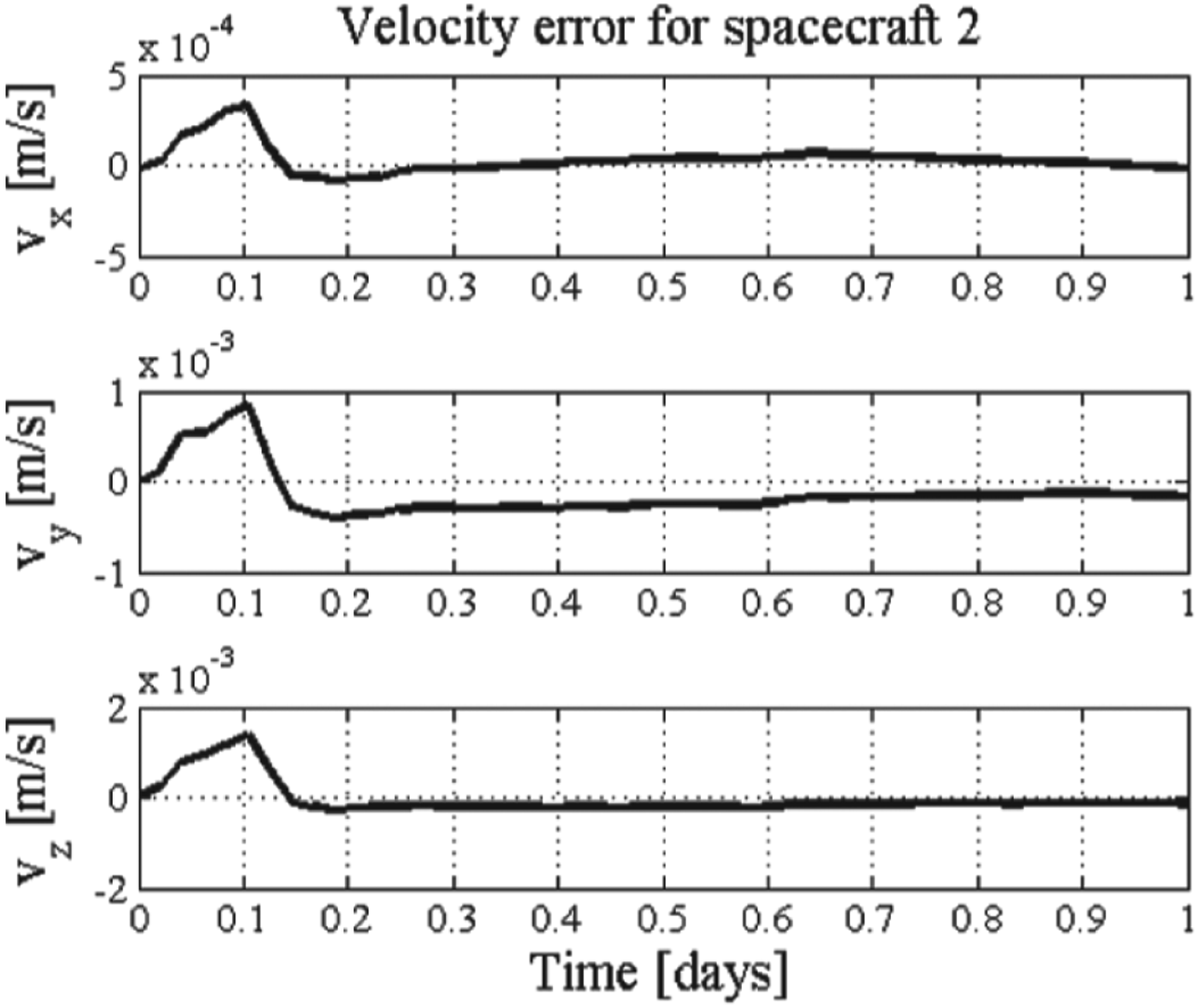
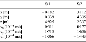
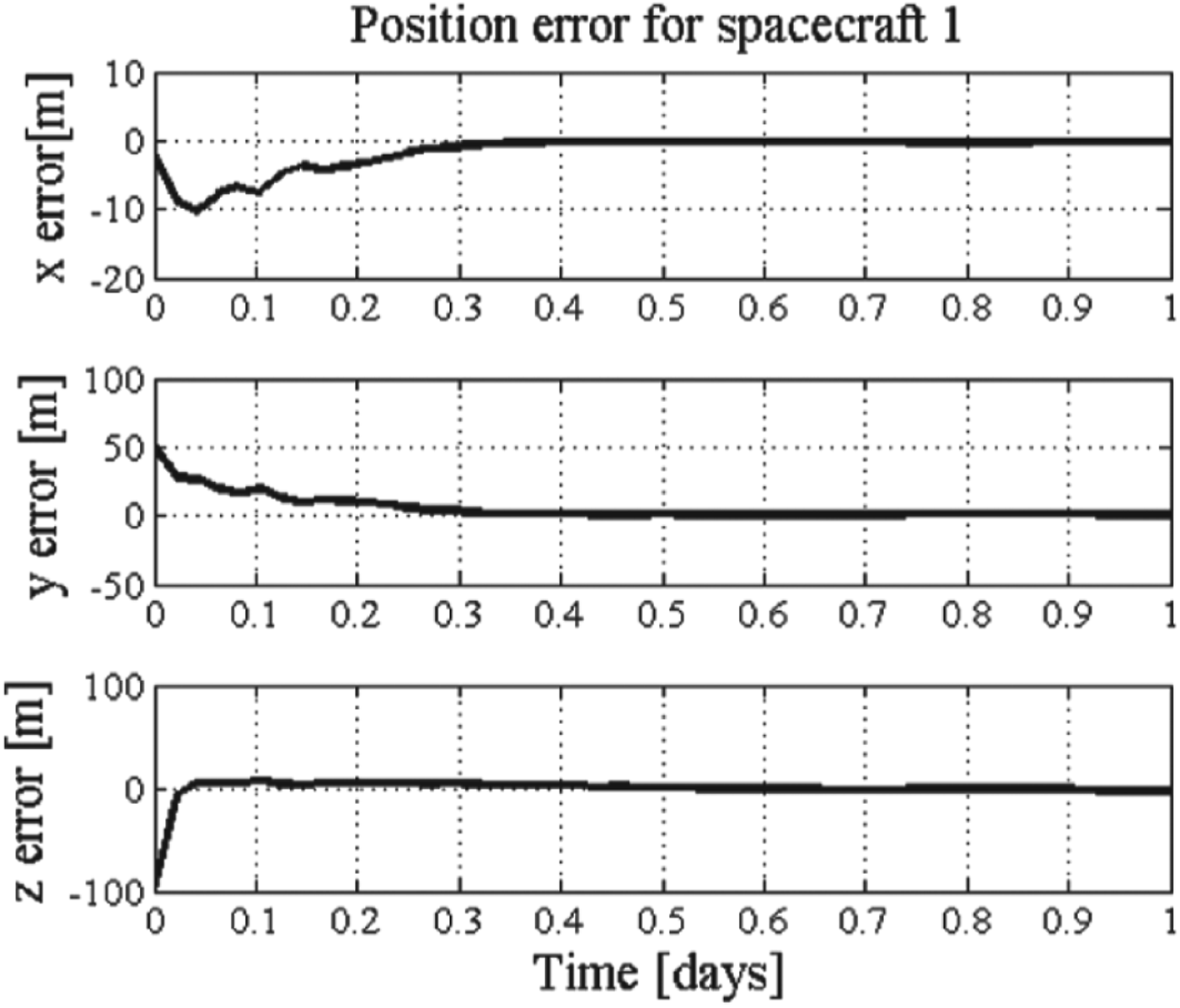
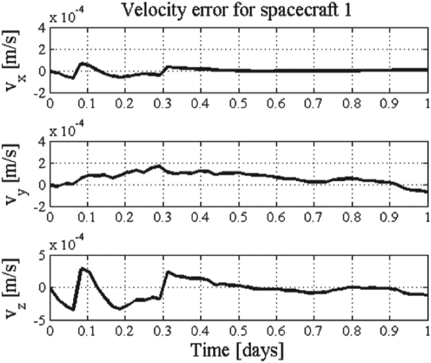
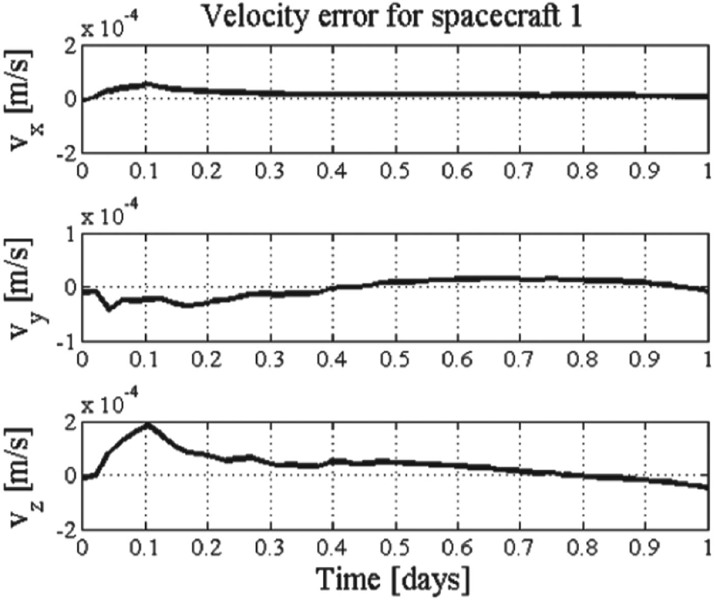
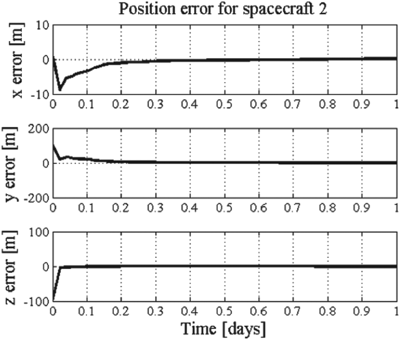
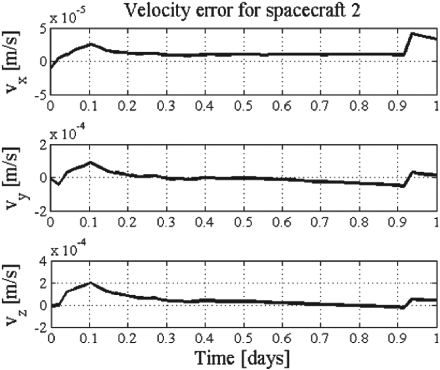
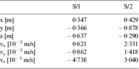
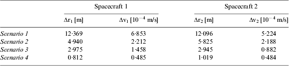
The estimated position and velocity errors in three directions of both spacecraft with respect to the Apophis are shown in Figures 9 and 10. The simulation results are summarized in Table 5 (based on ten runs). The position errors at the end of the simulation are about 12·369 m and 12·096 m of spacecraft one and two, respectively. The velocity errors at the final simulation are about 6·853×10−4 m/s and 5·224 ×10−4 m/s of spacecraft one and two, respectively. At about 0·4 day, the filters of both spacecraft become convergent.
Position errors of Scenario 1.
Velocity errors of Scenario 1.
Position errors of Scenario 1..
Velocity errors of Scenario 1.
Estimation errors for Scenario 1.
5.2. Scenario 2: Camera and LIDAR position measurements
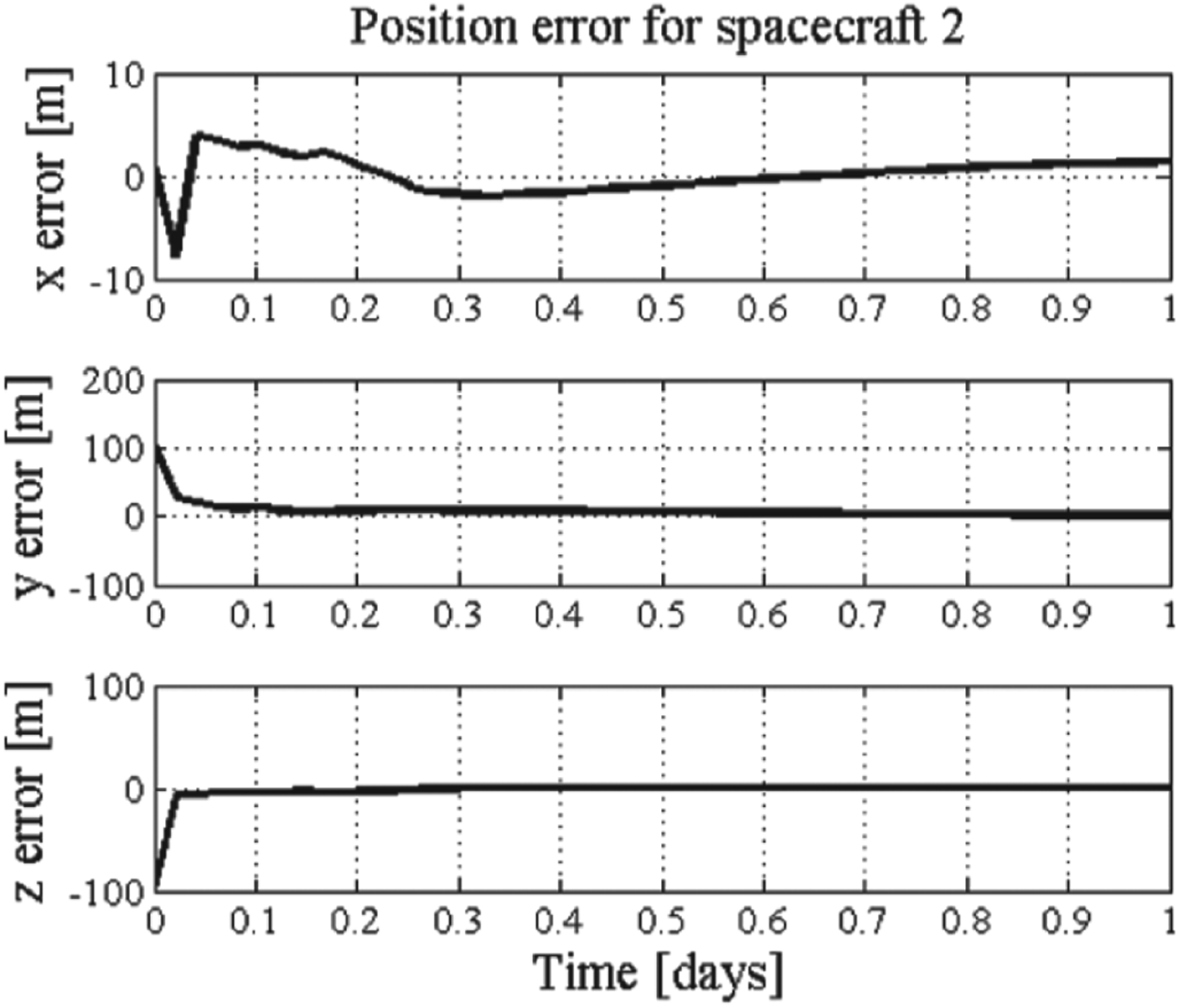
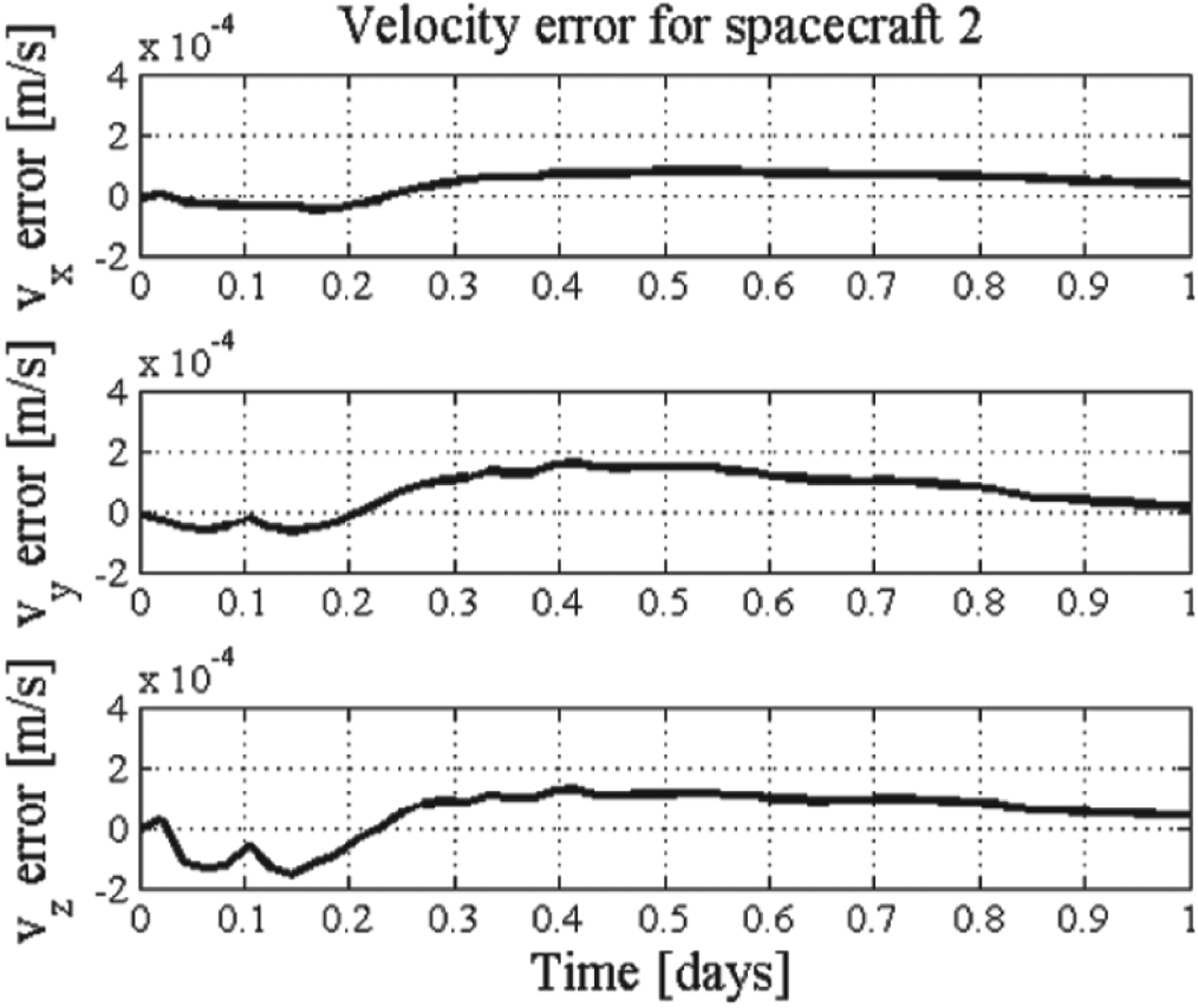
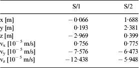
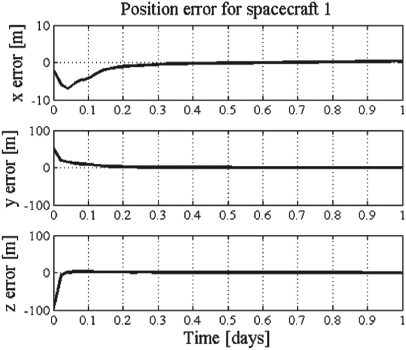
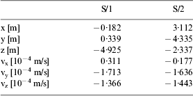
The estimation errors of position and velocity of the two spacecraft in each direction are shown in Figures 11 and 12, respectively. The navigation accuracy of the position and velocity of spacecraft one are better than 5 m and 5×10⁻⁴ m/s, respectively. The results are summarized in Table 6 (based on ten runs).
Position errors of Scenario 2.
Velocity errors of Scenario 2.
Position errors of Scenario 2.
Velocity errors of Scenario 2.
Estimation errors for Scenario 2.
5.3. Scenario 3: Spacecraft-to-asteroid measurements and Inter-range measurements
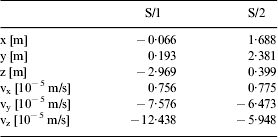
3-direction estimated position and velocity errors for Scenario 3 are plotted in Figures 13 and 14. Because the inter-range measurement is included in this scenario, the estimation accuracy is considerably improved with the position and velocity error less than 4 m and 2×10⁻⁴ m/s for spacecraft one, respectively. The accuracy of position and velocity for spacecraft two are better than 3 m and 2×10⁻⁴ m/s, respectively. The accuracies for each direction are summarized in Table 7 (based on ten runs).
Position errors of Scenario 3.
Velocity errors of Scenario 3.
Position errors of Scenario 3.
Velocity errors of Scenario 3.
Estimation errors for Scenario 3.
5.4. Scenario 4: Spacecraft-to-asteroid measurements and Inter-position measurements
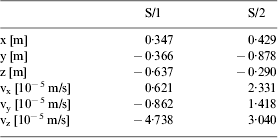
Simulation results can been seen in Figures 15 and 16; it is obvious that the performance of the filter is improved, with the accuracy of position better than 2 m and 1×10⁻⁴ m/s in velocity of spacecraft one. Similar improvements can be found for spacecraft two. Simulation results of both spacecraft are summarised in Table 8 (based on ten runs). The reasons for the improvements of the performance are the increased number of the measurements that makes the system more observable and the better quality of the inter-spacecraft measurements.
Position errors of Scenario 4.
Velocity errors of Scenario 4.
Position errors of Scenario 4.
Velocity errors of Scenario 4.
Estimation errors for Scenario 4.
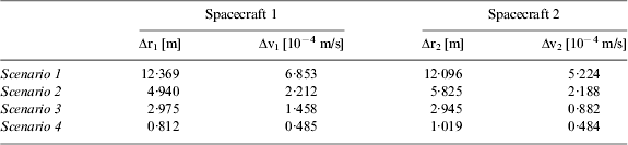
The total estimation errors of the four scenarios for both spacecraft are summarized in Table 9. Up to 90% improvements are achieved in the position and velocity estimated accuracy for both spacecraft by comparing Scenario 4 to Scenario 1. Comparing with Scenarios 2, 3 and 4 this illustrates that although the magnitude of the improvements is not that overwhelming, the filter performance is improved when inter-spacecraft measurements are added into the measurement model. Another conclusion can be drawn that the angular measurements make the greater contribution to improvement in both non-collaborative and collaborative scenarios.
Trajectory's estimated errors after one day, based on 10 runs.
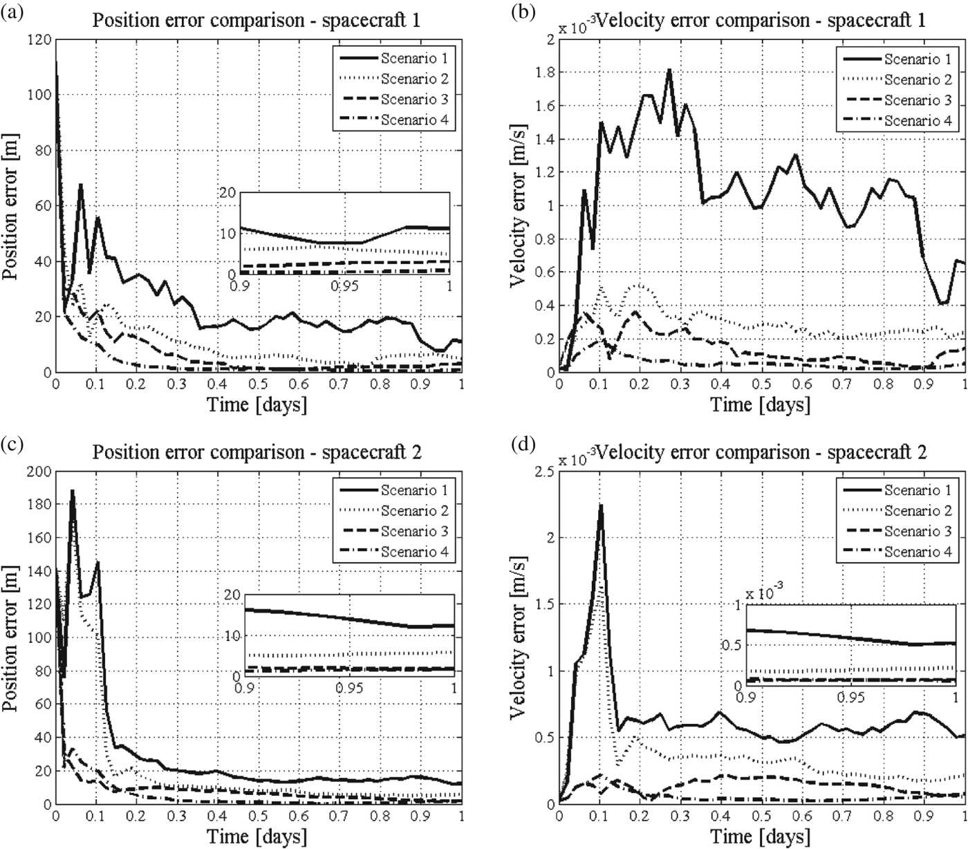
Comparisons of the behaviours of the relative position and velocity error estimation of the four scenarios are shown in Figures 17(a) (b) (c) and (d), for the two spacecraft, respectively. The enlarged areas in the figures clearly show the estimated accuracy at the end of the simulation.
Comparisons of four scenarios (a) position errors of spacecraft one, (b) velocity errors of spacecraft 1 and (c) position errors of spacecraft 2, (d) velocity errors of spacecraft two.
It is obvious that the filter in Scenario 2 converges better than Scenario 1 at the first few steps of the simulation. In addition, the final estimated accuracies are 4·940 m in position and 2·212×10−4 m/s in velocity, which are better than the results of Scenario 1. Similar results can be concluded for spacecraft two. The comparison between Scenarios 2 and 3 indicates that the inter-range measurement improves the orbit determination accuracy. At the end of simulation, the position error of spacecraft one is 2·975 m and the velocity error is 1·458×10−4 m/s. The filter converges more rapidly with better steady-state estimation performance in Scenario 3 for both spacecraft.
Scenario 4 is compared with Scenario 3 to illustrate the improvement in the estimated accuracy for both spacecraft. Particularly, for spacecraft two, the position and velocity errors are worse than Scenario 3 until 0·1 day. After that, the convergence and the final accuracy in Scenario 4 are better than Scenario 3, which is 1·019 m and 0·484×10−4 m/s in position and velocity errors, respectively, while the estimated errors of Scenario 3 are 2·945 m in position and 0·882×10−4 m/s in velocity at the end of the simulation.
It can be seen that the non-collaborative Scenario 1 and Scenario 2 are less precise than the collaborative Scenario 3 and Scenario 4. The accuracy of orbit determination of both spacecraft are improved in the aspects of stability and convergence properties by increasing the number of the measurements and combining the available inter-spacecraft measurements to the measurement model.
6. CONCLUSIONS
This paper has studied the orbit determination method for a two-spacecraft formation flying in the proximity of a slowly rotating asteroid by fusing the spacecraft-to-asteroid and inter-spacecraft observations in the UKF-based autonomous orbit determination algorithm. Simulation results indicate that the position error is in the range of metres and the velocity error is in the range of 10−4 m/s. The camera and LIDAR are proved to be effective by building up the integrated measurement models. Good quality inter-spacecraft angular measurements made noticeable improvements in the orbit determination accuracy. Collaborative scenarios with inter-spacecraft position vector measurements achieved the best performance.
In the future studies, the robustness of the collaborative orbit determination scenarios should be analysed by comparing several working situations of the sensors. Sensitivity of the measurement and process noise to system performance will be studied to better understand how the filter is affected.
ACKNOWLEDGEMENTS
The authors thank Prof. M. Vasile and Mr. M. Vertrisano from the Advanced Space Concepts Laboratory of University of Strathclylde, UK, for their supervision throughout the work. The work is partially supported by National Natural Science Foundation of China under Grant No. 11102229, Hunan Provincial Innovation Foundation For Postgraduate under Grant No. CX2011B004, and Fund of Innovation by Graduate School of National University of Defense Technology under Grant No. B110104.