

1 Introduction
A jet in cross-flow (JICF) or transverse jet typically consists of a round jet issuing perpendicularly into cross-flow. This canonical three-dimensional flow field has been studied for many decades, in part because of its extensive applications to engineering propulsion systems (Karagozian Reference Karagozian2010). The interaction between the jet and cross-flow generates diverse vortical structures, including the well-known counter-rotating vortex pair (CVP), shown schematically in figure 1(a). The jet-to-cross-flow density ratio,  $S\equiv \unicode[STIX]{x1D70C}_{j}/\unicode[STIX]{x1D70C}_{\infty }$, velocity ratio,
 $R\equiv U_{j}/U_{\infty }$, and momentum flux ratio,
 $J\equiv \unicode[STIX]{x1D70C}_{j}U_{j}^{2}/\unicode[STIX]{x1D70C}_{\infty }U_{\infty }^{2}$, are among the non-dimensional parameters often used in studying JICF behaviour, in addition to the jet Reynolds number,
 $Re_{j}\equiv \unicode[STIX]{x1D70C}_{j}U_{j}D/\unicode[STIX]{x1D707}_{j}$, which is based on the mean jet exit velocity
 $U_{j}$, jet diameter
 $D$ and the absolute viscosity of the jet fluid,
 $\unicode[STIX]{x1D707}_{j}$. A Strouhal number
 $St_{o}\equiv f_{o}D/U_{j}$ non-dimensionalizes frequencies associated with the fundamental upstream shear layer (USL) instability corresponding to initial vortex rollup (Getsinger et al. Reference Getsinger, Gevorkyan, Smith and Karagozian2014). Alternative length scales that can be used in the definition of Strouhal number include momentum thicknesses for the jet fluid as well as the USL; this scaling will be discussed later in detail.
(a) Schematic of a flush-injected JICF, including orientation of coordinate axes  $x$,
 $y$,
 $z$, and jet USL trajectory
 $s$ (adapted from Fric & Roshko (Reference Fric and Roshko1994)). (b) Schematic of the effect of jet blockage of cross-flow, creating local negative velocity
 $V_{2}$ upstream of the USL adjacent to a positive vertical velocity
 $V_{1}$ within the jet (adapted from Iyer & Mahesh (Reference Iyer and Mahesh2016)).

The transverse jet’s USL is known to transition from being convectively unstable at larger  $J$ values to being absolutely or globally unstable at smaller
 $J$. There is extensive experimental evidence for this transition, for both equidensity (Megerian et al. Reference Megerian, Davitian, Alves and Karagozian2007; Davitian et al. Reference Davitian, Getsinger, Hendrickson and Karagozian2010) and low-density (Getsinger, Hendrickson & Karagozian Reference Getsinger, Hendrickson and Karagozian2012) jets in cross-flow. For the equidensity JICF in which nitrogen is injected from a nozzle that is flush with respect to the injection wall into a cross-flow of air, at both
 $Re_{j}=2000$ and
 $3000$, hot-wire-based studies determine that the USL transition from convective to absolute instability occurs when increasing cross-flow velocity causes the jet-to-cross-flow velocity ratio to fall below a critical value of
 $R\approxeq 3.1$. For low-density transverse jets consisting of mixtures of nitrogen and helium injected into air from a flush nozzle, the transition to absolute instability is documented in Getsinger et al. (Reference Getsinger, Hendrickson and Karagozian2012) to occur for momentum flux ratio
 $J\lesssim 10$ and/or density ratio
 $S\lesssim 0.40$, the latter of which is consistent with low-density free-jet studies in this Reynolds-number regime (Hallberg & Strykowski Reference Hallberg and Strykowski2006). At these relatively low
 $R$ or
 $J$ values, the transverse jet can be deflected considerably by the cross-flow, causing a slowly varying parallel flow approximation, which works well in a local linear stability analysis (LSA) of the flow for
 $J>10$ (Alves, Kelly & Karagozian Reference Alves, Kelly and Karagozian2007, Reference Alves, Kelly and Karagozian2008), to be less appropriate for the USL. Global LSA for the JICF at lower velocity or momentum flux ratios (e.g.
 $J<10$), however, has shown success in demonstrating sustained self-excited global oscillations in the deflected transverse jet’s USL (Bagheri et al. Reference Bagheri, Schlatter, Schmid and Henningson2009; Peplinski, Schlatter & Henningson Reference Peplinski, Schlatter and Henningson2015; Regan & Mahesh Reference Regan and Mahesh2017).
Direct numerical simulations (DNS) by Iyer & Mahesh (Reference Iyer and Mahesh2016) for the equidensity JICF using the same flush nozzle geometry as in the experiments of Megerian et al. (Reference Megerian, Davitian, Alves and Karagozian2007), for the cases  $R=4$ and
 $2$ at
 $Re_{j}=2000$, show remarkably good qualitative and quantitative agreement in predicted spectral characteristics (e.g.
 $St_{o}$ values) for the jets based on vertical velocity disturbances along the USL. Additional experimental studies utilizing a flush round pipe for the equidensity JICF (Getsinger et al. Reference Getsinger, Gevorkyan, Smith and Karagozian2014) demonstrate a transition to absolute/global instability in the jet’s USL for
 $J\lesssim 10$, also observed in DNS (Bagheri et al. Reference Bagheri, Schlatter, Schmid and Henningson2009), although convective instabilities at higher
 $J$ values in the experiments are considerably weaker than for flush nozzle-injected jets. Further experiments involving optical diagnostics enable detailed study of the relationships among JICF shear layer instabilities, flow structure, molecular mixing and dynamical characteristics (Getsinger et al. Reference Getsinger, Gevorkyan, Smith and Karagozian2014; Gevorkyan et al. Reference Gevorkyan, Shoji, Getsinger, Smith and Karagozian2016, Reference Gevorkyan, Shoji, Peng and Karagozian2018).
Computations by Iyer & Mahesh (Reference Iyer and Mahesh2016) also investigate the similarity in the JICF USL instability transition to that of a two-dimensional (2-D) counter-current shear layer (CCSL), where the signs of the velocities of the two streams oppose one another. As indicated schematically in figure 1(b), cross-flow blockage by the jet can create a stagnation streamline and reverse flow region just outside of the USL near injection, creating a negative velocity  $V_{2}<0$ analogous to that in a CCSL, contrasting a positive vertical flow within the jet,
 $V_{1}>0$. The stagnation streamline generally appears well outside of the cross-flow wall boundary layer, even at large velocity ratios (Megerian et al. Reference Megerian, Davitian, Alves and Karagozian2007). In general a CCSL may be characterized by a mixing or shear layer ratio
 $R_{1}$ based on the velocities
 $V_{1}$ and
 $V_{2}$ shown in figure 1(b),
 $$\begin{eqnarray}\displaystyle R_{1}=\frac{V_{1}-V_{2}}{V_{1}+V_{2}}, & & \displaystyle\end{eqnarray}$$
so that  $R_{1}>1.0$ denotes counter-flow and
 $R_{1}<1.0$ denotes co-flow. Inviscid spatio-temporal stability analysis of an incompressible, planar CCSL using a hyperbolic tangent velocity profile (Huerre & Monkewitz Reference Huerre and Monkewitz1985) indicates that the CCSL becomes absolutely unstable when
 $R_{1}$ exceeds a critical value,
 $R_{1,cr}=1.315$. Corresponding experiments for an axisymmetric (round) jet with a finite region of exterior suction (Strykowski & Niccum Reference Strykowski and Niccum1991) suggest a critical velocity ratio very close to the theoretical value,
 $R_{1,cr}\approx 1.32$. Similar inviscid LSA for the compressible planar CCSL, with streams of differing densities, has also been performed (Pavithran & Redekopp Reference Pavithran and Redekopp1989), employing the Crocco–Busemann relation and an equation of state for a perfect gas. Corresponding axisymmetric counter-current jet experiments by Strykowski & Niccum (Reference Strykowski and Niccum1992) quantify values of
 $R_{1,cr}$ for various density ratios
 $S$. For the equidensity round transverse jet, Iyer & Mahesh (Reference Iyer and Mahesh2016) utilize DNS-generated velocity fields in the USL to compute the effective shear layer ratio
 $R_{1}$ just downstream of jet injection. In the
 $R=4$ case,
 $R_{1}$ is estimated in the centre plane (
 $y=0$ plane) to be 1.2, while for the
 $R=2$ simulation,
 $R_{1}=1.44$. Even with the simplified parallel flow approximation for the JICF at the low velocity ratio, the findings suggest that these two different JICF flow conditions could straddle the transition between convective and absolute instability when viewed in the context of a local CCSL occurring at the upstream edge of flush JICF injection. Despite the relatively limited extent of both the negative and positive velocity regions for the flush nozzle-generated JICF, the CCSL model appears to be consistent with instability differences for these two transverse jet cases.
The compelling nature of this analogy for transition in the transverse jet’s shear layer instabilities, coupled with recent observations on differences in the transition conditions based on fluid species present in the jet, has motivated the present examination. Data from a rather wide range of experimental flow conditions can be used in exploring the analogy as a means of exploring the nature of the transition and understanding the physics of its origins.
2 Experimental configuration
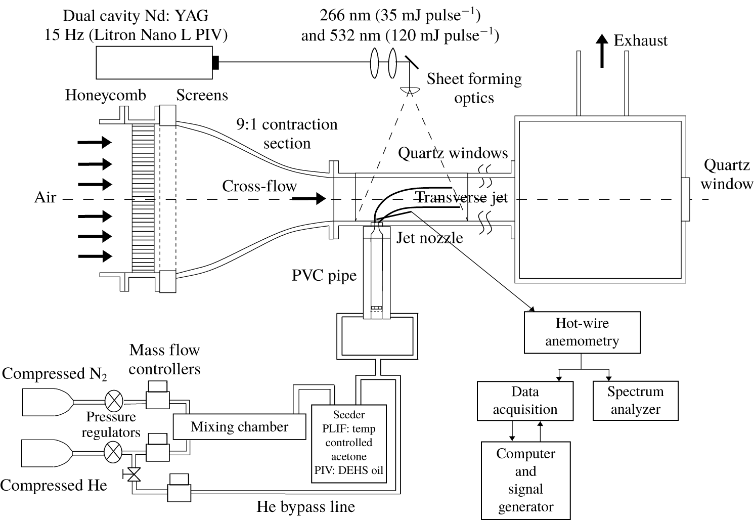
Low-velocity wind tunnel with associated hot-wire anemometry and optical diagnostic apparatus. One additional tunnel section, of identical dimensions, was situated downstream of the test section shown.

This experimental study on gaseous jets in cross-flow utilized a low-velocity wind tunnel with hot-wire anemometry for spectral characterization and laser diagnostics for scalar and velocity field quantification. The experimental configuration is shown in figure 2. Details on the set-up and optical diagnostics are available in recent papers (Getsinger et al. Reference Getsinger, Gevorkyan, Smith and Karagozian2014; Gevorkyan et al. Reference Gevorkyan, Shoji, Getsinger, Smith and Karagozian2016, Reference Gevorkyan, Shoji, Peng and Karagozian2018), but a brief overview is provided here. A cross-flow of air in the downstream (positive  $x$) direction was created by a centrifugal blower placed upstream of the test section, which had dimensions
 $30~\text{cm}\times 12~\text{cm}\times 12~\text{cm}$. The turbulence intensity in the tunnel-generated cross-flow in the absence of the jet was less than 1.5 % of the maximum achievable cross-flow velocity of approximately
 $7~\text{m}~\text{s}^{-1}$. A Plexiglas window fitted into the side of the test section enabled optical access for laser diagnostics in the centre plane (
 $y=0$ or
 $x{-}z$ plane in figure 1a).
This study primarily utilized jets issuing perpendicularly into cross-flow from a fifth-order polynomial nozzle with a  $64:1$ area ratio contraction, mounted flush to the bottom floor of the test section and with an exit diameter
 $D=4.04~\text{mm}$ (referenced as the ‘flush nozzle’). For one dataset, a fifth-order polynomial nozzle with the same contraction ratio and
 $D=7.59~\text{mm}$ (the ‘larger flush nozzle’) was examined. Each created a top-hat-like velocity profile with a thin jet boundary layer in the absence of cross-flow (e.g. as documented in Megerian et al. (Reference Megerian, Davitian, Alves and Karagozian2007)). The jet fluid comprised mixtures of helium and nitrogen and, for cases involving laser diagnostics, tracer species. For optical diagnostics, the jet fluid flowed into a temperature-controlled acetone seeder for planar laser-induced fluorescence (PLIF) imaging of the acetone, which was maintained in the vapour phase, and/or into a particle seeder for stereo particle image velocimetry (PIV) measurements. The jet Reynolds number could be fixed, while density ratios were varied in the range
 $0.35\leqslant S\leqslant 1.00$. Adjusting the mole fractions of various species enabled the desired densities and jet Reynolds numbers to be achieved (Gevorkyan et al. Reference Gevorkyan, Shoji, Getsinger, Smith and Karagozian2016, Reference Gevorkyan, Shoji, Peng and Karagozian2018). Jet density and viscosity were calculated considering all constituents in the jet, with or without inclusion of the acetone mole fraction
 $\unicode[STIX]{x1D713}$, depending on experimental conditions. The viscosity of the jet was determined by the Wilke formulation without acetone vapour in the jet (Bird, Stewart & Lightfoot Reference Bird, Stewart and Lightfoot1960) and by the Reichenberg method with acetone (Poling, Prausnitz & O’Connell Reference Poling, Prausnitz and O’Connell2001). The desired momentum flux ratio was achieved by varying the cross-flow velocity
 $U_{\infty }$ for fixed
 $S$ and
 $Re_{j}$; the present studies focused on the range
 $3\leqslant J\leqslant 61$. As per the analysis in Canzonieri (Reference Canzonieri2009), the maximum experimental uncertainty in jet density was 1.5 % in the absence of acetone. With acetone present, the additional sources of error associated with the pressure and temperature control for the acetone seeder produced a maximum uncertainty of 5.1 % in jet density (Shoji Reference Shoji2017).
These experiments utilized constant-temperature hot-wire anemometry (Dantec 55P15), either with or without acetone vapour seeded in the jet, enabling spectral measurements of the transverse jet’s USL to be made. A single-component, boundary-layer-type hot-wire probe was used with a triple-axis linearly staged platform to control position to within  $1~\unicode[STIX]{x03BC}\text{m}$ accuracy. Spectral data were fed to a dual-channel dynamic signal analyser (HP Model 35665A) and averaged over 40 instantaneous frequency distributions. The spectral measurements were applied over a 6.4 kHz range with 8 Hz resolution. Separately, stereo PIV measurements were utilized in the jet centre plane to acquire velocity fields in a non-intrusive manner. Besides PIV-only data, velocity data were acquired via the PIV portion of simultaneous stereo PIV and acetone PLIF imaging. A dual-cavity Q-switched Nd:YAG laser (Litron Nano L PIV) was employed in most of the studies with second- and fourth-harmonic generators to generate concentric 532 nm and 266 nm wavelength light for PIV and PLIF imaging, respectively. Each cavity was able to produce a 8 ns full width at half-maximum (FWHM) pulse, with 30 mJ at 266 nm and 120 mJ at 532 nm, at a maximum repetition rate of 15 Hz, although the repetition rate used in actual measurements was typically 1 Hz, as discussed in detail in prior studies (Getsinger et al. Reference Getsinger, Gevorkyan, Smith and Karagozian2014; Gevorkyan et al. Reference Gevorkyan, Shoji, Getsinger, Smith and Karagozian2016, Reference Gevorkyan, Shoji, Peng and Karagozian2018). A few additional datasets were taken here with a Quantel Evergreen 30266 Nd:YAG laser with similar characteristics.
Diethyl hexyl sebacate (DEHS) oil was utilized for seeding the jet flow in PIV experiments by diverting part of the jet fluid injection line through a TSI particle generator. For the cross-flow, a commercial fog machine (Pea Soup Rocket) atomized and then injected glycol-based smoke fluid particles of  $0.2~\unicode[STIX]{x03BC}\text{m}$ mass-median diameter into the cross-flow blower inlet. For simultaneous PLIF and PIV measurements, in addition to DEHS oil, acetone was seeded into the jet via two acetone seeder chambers placed upstream of the jet injection system, capable of seeding acetone tracer into the jet fluid in the gas phase at the desired mole fraction,
 $\unicode[STIX]{x1D713}$. The second chamber temperature was controlled within the range of
 $3{-}18\,^{\circ }\text{C}$, creating an acetone vapour mole fraction range of
 $\unicode[STIX]{x1D713}$ up to approximately 0.218, varied to achieve the desired fluorescence intensity for the different gas mixtures utilized in the study. Imaging for the stereo PIV system comprised two 14-bit charge-coupled device (CCD) cameras (LaVision Imager proX,
 $1600\times 1200$ pixel resolution) separated by an approximate
 $60^{\circ }$ angle with respect to the
 $z$ axis. Each camera was equipped with a Nikon 60 mm lens at
 $f/11.0$, a 532.5 nm narrowband filter and a Scheimpflug lens mount; this resulted in an in-plane pixel size of approximately
 $120~\unicode[STIX]{x03BC}\text{m}$ for PIV studies, finer than the strain-limited diffusion scale for all flow conditions in the present study (Gevorkyan et al. Reference Gevorkyan, Shoji, Peng and Karagozian2018). The temporal interval of the two laser pulses was in the range
 $4{-}17.5~\unicode[STIX]{x03BC}\text{s}$, depending on flow conditions, to achieve reasonable correlation between two frames over the entire field of view. Further details on the experimental configuration and laser diagnostics may be found in Shoji (Reference Shoji2017) and Gevorkyan et al. (Reference Gevorkyan, Shoji, Peng and Karagozian2018).
3 Results
3.1 Shear layer instabilities for different jet mixtures
Prior experimental studies provide extensive evidence that the USL for the equidensity flush nozzle-injected JICF, consisting of pure  $\text{N}_{2}$ injected into air, becomes globally unstable when
 $J$ is brought to or below
 $J_{cr}\approx 10$ (Megerian et al. Reference Megerian, Davitian, Alves and Karagozian2007; Davitian et al. Reference Davitian, Getsinger, Hendrickson and Karagozian2010), or that the low-density JICF consisting of He–
 $\text{N}_{2}$ mixtures becomes absolutely/globally unstable when
 $J\lesssim 10$ and/or
 $S\lesssim 0.40$ (Getsinger et al. Reference Getsinger, Hendrickson and Karagozian2012). Among the most compelling pieces of evidence for this transition is the significant alteration in hot-wire-based USL spectral characteristics with changes in flow conditions, although there are many additional documented features associated with this transition (Davitian et al. Reference Davitian, Getsinger, Hendrickson and Karagozian2010). The hot wire is traversed along the USL trajectory coordinate
 $s/D$ (see figure 1), determined based on a power-law fit to the maximum gradient in the local vertical velocity field. For the low-density JICF (
 $S<1$) and hence for continuously varying density fields, which present difficulties in hot-wire velocity calibration, the USL trajectory as well as spectral characteristics may be determined based on uncalibrated hot-wire voltage (Getsinger et al. Reference Getsinger, Hendrickson and Karagozian2012) since the uncalibrated hot-wire signal still yields the same frequency content at various locations as a calibrated hot wire.
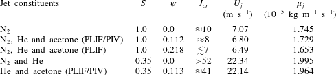
For various jet gas constituents with increasing acetone mole fraction,  $\unicode[STIX]{x1D713}$, shown are mean jet velocity and absolute viscosity required for matching
 $Re_{j}=1900$ for two different density ratios,
 $S=1.0$ and 0.35. Values of the estimated critical momentum flux ratio
 $J_{cr}$ based on hot-wire measurements are also given.

In the present experiments, spectral characteristics of the JICF were acquired via hot-wire anemometry for the same overall flow conditions ( $Re_{j}$,
 $J$,
 $S$) but with different mixtures of species in the jet fluid. These mixtures corresponded to experiments employing different optical diagnostics. Relevant parameters are quantified in table 1 for both equidensity and low-density (
 $S=0.35$) flush nozzle-injected jets for the case
 $Re_{j}=1900$. Gas constituents included pure nitrogen associated with earlier equidensity experiments (Megerian et al. Reference Megerian, Davitian, Alves and Karagozian2007; Getsinger et al. Reference Getsinger, Hendrickson and Karagozian2012) and mixtures of nitrogen and helium with acetone for simultaneous PLIF/PIV (
 $\unicode[STIX]{x1D713}=0.112$) and for higher-resolution PLIF-only experiments (
 $\unicode[STIX]{x1D713}=0.218$) typically used to quantify molecular mixing (Gevorkyan et al. Reference Gevorkyan, Shoji, Getsinger, Smith and Karagozian2016). Gas constituents corresponding to the simultaneous PLIF/PIV experiments did not include DEHS oil so as to enable hot-wire usage for spectral measurements.
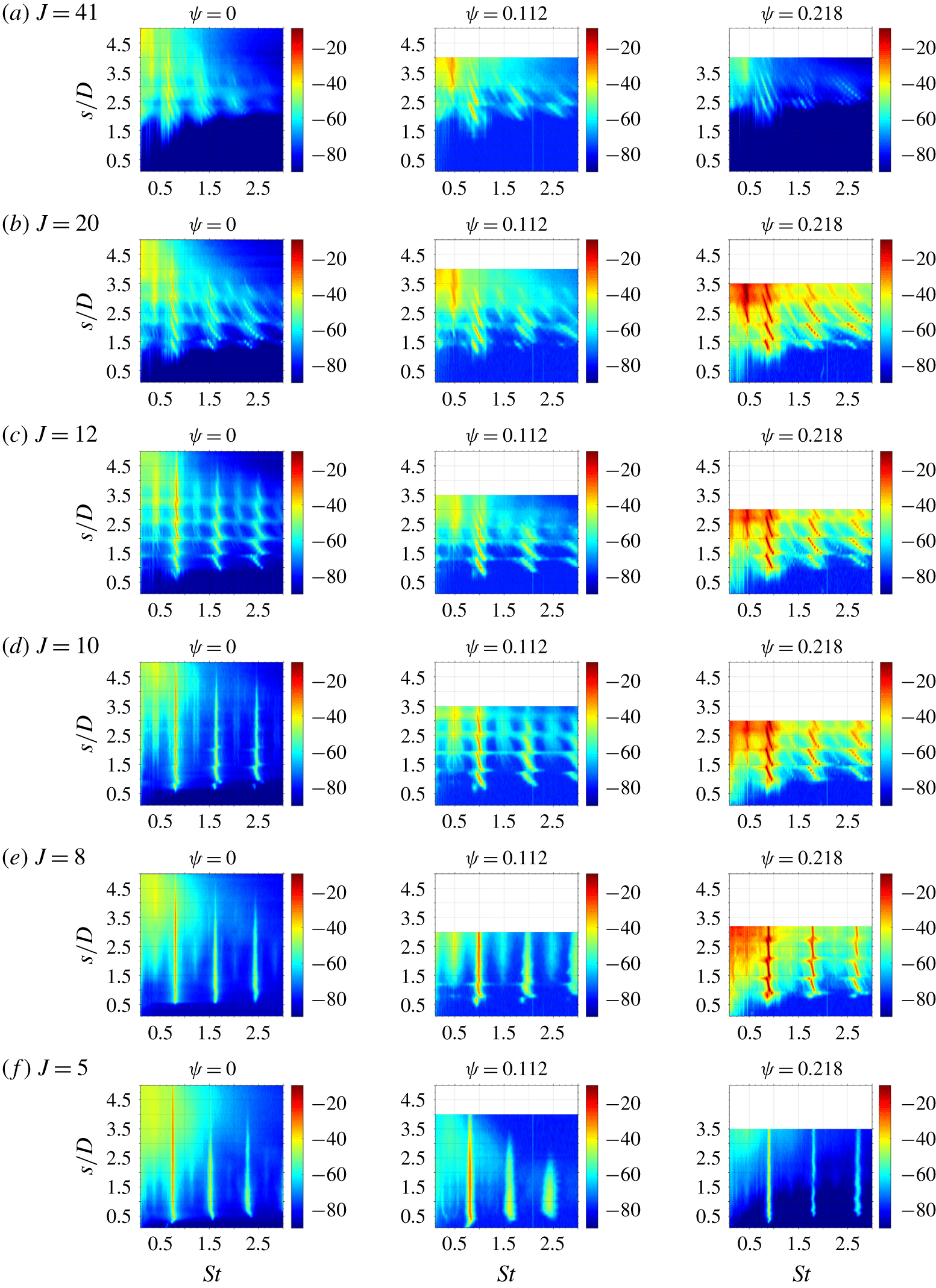
Figure 3 shows fine-resolution spectral magnitude contour plots for the equidensity JICF, representing the hot-wire response to vertical velocity fluctuations measured along the USL trajectory  $s/D$, for a fixed jet Reynolds number (
 $Re_{j}=1900$) with different momentum flux ratios
 $J$. Data are shown for different mixtures of species in the jet fluid, corresponding to different mole fractions of acetone:
 $\unicode[STIX]{x1D713}=0$ for the pure
 $\text{N}_{2}$ jet (approximately the same as for PIV-only experiments),
 $\unicode[STIX]{x1D713}=0.0112$ for typical simultaneous PLIF/PIV experimental conditions and
 $\unicode[STIX]{x1D713}=0.218$ for the typical PLIF-only experiments. Interestingly, while the overall change in USL spectral characteristics from convectively unstable (CU) behaviour at
 $J=41$ to absolutely unstable (AU) or globally unstable (GU) behaviour at
 $J=5$ was similar, there were subtle differences as transition from CU to AU took place, based on
 $\unicode[STIX]{x1D713}$. Interestingly, despite the careful matching of
 $Re_{j}$,
 $S$ and
 $J$ values here, the mixture of constituent gases in the jet affected the evolution of USL, both qualitatively and quantitatively. This observation will be discussed and explored further below. At
 $J=41$,
 $20$ and
 $12$, multiple spatially evolving instabilities in the USL were observed, with frequency shifting along the trajectory
 $s/D$ resulting from tonal interference between the successively strengthening shear layer instability and the hot-wire probe (Hussain & Zaman Reference Hussain and Zaman1978; Getsinger et al. Reference Getsinger, Hendrickson and Karagozian2012). The average of the shifting frequencies was considered to correspond to a fundamental frequency
 $f_{o}$, as done in prior studies (Megerian et al. Reference Megerian, Davitian, Alves and Karagozian2007; Davitian et al. Reference Davitian, Getsinger, Hendrickson and Karagozian2010; Getsinger et al. Reference Getsinger, Hendrickson and Karagozian2012). Subharmonic development, representing vortex merger, was more prominent at these higher
 $J$ values, while higher harmonics appeared to be strengthened with a reduction in
 $J$ as cross-flow velocity
 $U_{\infty }$ increased. These spectral characteristics corresponded to the behaviour of a convectively unstable USL, as discussed in prior JICF stability studies (Megerian et al. Reference Megerian, Davitian, Alves and Karagozian2007; Davitian et al. Reference Davitian, Getsinger, Hendrickson and Karagozian2010; Getsinger et al. Reference Getsinger, Hendrickson and Karagozian2012). But with the addition of increasing concentrations of acetone, and with the presence of helium and nitrogen designed to create
 $S=1$, the location of initiation of the instability (
 $s/D$) was delayed, especially as
 $J$ was reduced, suggesting a slight weakening of the shear layer instability with increasing acetone concentration. There were also increases in the estimated average fundamental frequency
 $f_{o}$ and hence Strouhal number
 $St_{o}$ associated with the initiation of the instability as
 $\unicode[STIX]{x1D713}$ was increased.
Spectral contour maps of the hot-wire-based velocity disturbances along the USL trajectory coordinate  $s/D$ for the JICF at
 $Re_{j}=1900$ and
 $S=1.0$ with varying
 $J$ and acetone mole fraction
 $\unicode[STIX]{x1D713}$, corresponding to jets with
 $\text{N}_{2}$ only (
 $\unicode[STIX]{x1D713}=0$, reproduced from original data in Getsinger et al. (Reference Getsinger, Hendrickson and Karagozian2012)), the jet mixture for simultaneous PLIF and PIV (
 $\unicode[STIX]{x1D713}=0.112$) and the PLIF-only experiments (
 $\unicode[STIX]{x1D713}=0.218$). The colour bar represents disturbance amplitude in dB.

As the momentum flux ratio was reduced to the range close to initiation of an absolutely unstable USL for the pure nitrogen jet, near  $J=10$ (Megerian et al. Reference Megerian, Davitian, Alves and Karagozian2007; Davitian et al. Reference Davitian, Getsinger, Hendrickson and Karagozian2010; Getsinger et al. Reference Getsinger, Hendrickson and Karagozian2012), figure 3(d) indicates that the effect of acetone in the jet mixture was not only to delay the onset of the instability, but to cause its characteristics to be associated with convective instability rather than the pure-tone, spatially invariant absolute instability observed for
 $\unicode[STIX]{x1D713}=0$ at this flow condition. Even at
 $J=8$ (figure 3e), there was evidence of a weakening of the shear layer, with a very low level of tonal interference, especially at
 $\unicode[STIX]{x1D713}=0.218$, which typically would not be classified as characteristic of GU flow. At a much lower value of
 $J=5$, shown in figure 3(f), all jet mixtures produced the typical AU/GU behaviour, with a strong pure-tone instability initiated close to the jet exit, a clear fundamental frequency
 $f_{o}$ and the absence of subharmonic disturbances. For these lower
 $J$ values there were nevertheless small increases in
 $St_{o}$ with increasing
 $\unicode[STIX]{x1D713}$.
To verify that the phenomena observed in figure 3 reflected actual USL behaviour and that acetone itself was not affecting hot-wire performance, spectral measurements were also made outside of the USL, where there was little or no acetone present. For these spectral measurements the hot-wire probe was initially situated at a fixed USL trajectory location then traversed upstream, in the negative  $x$ direction, fixing
 $y$ and
 $z$ locations. There were no substantive alterations in spectral character (other than strength of the instabilities) as the hot wire was moved outside of the USL into the air cross-flow and, in addition,
 $St_{o}$ did not vary. Thus it was determined that alterations in the USL transition and
 $J_{cr}$ for the acetone-seeded JICF reflected actual physical phenomena and were not affected by the measurement method.
Similar alterations in fundamental  $St_{o}$ values and
 $J_{cr}$ were observed in other acetone-seeded JICF experiments for a range of operating conditions, where deviations from established values of
 $J_{cr}$ occurred when acetone was present in the jet fluid. Yet overall trends associated with the variation in
 $St_{o}$ with
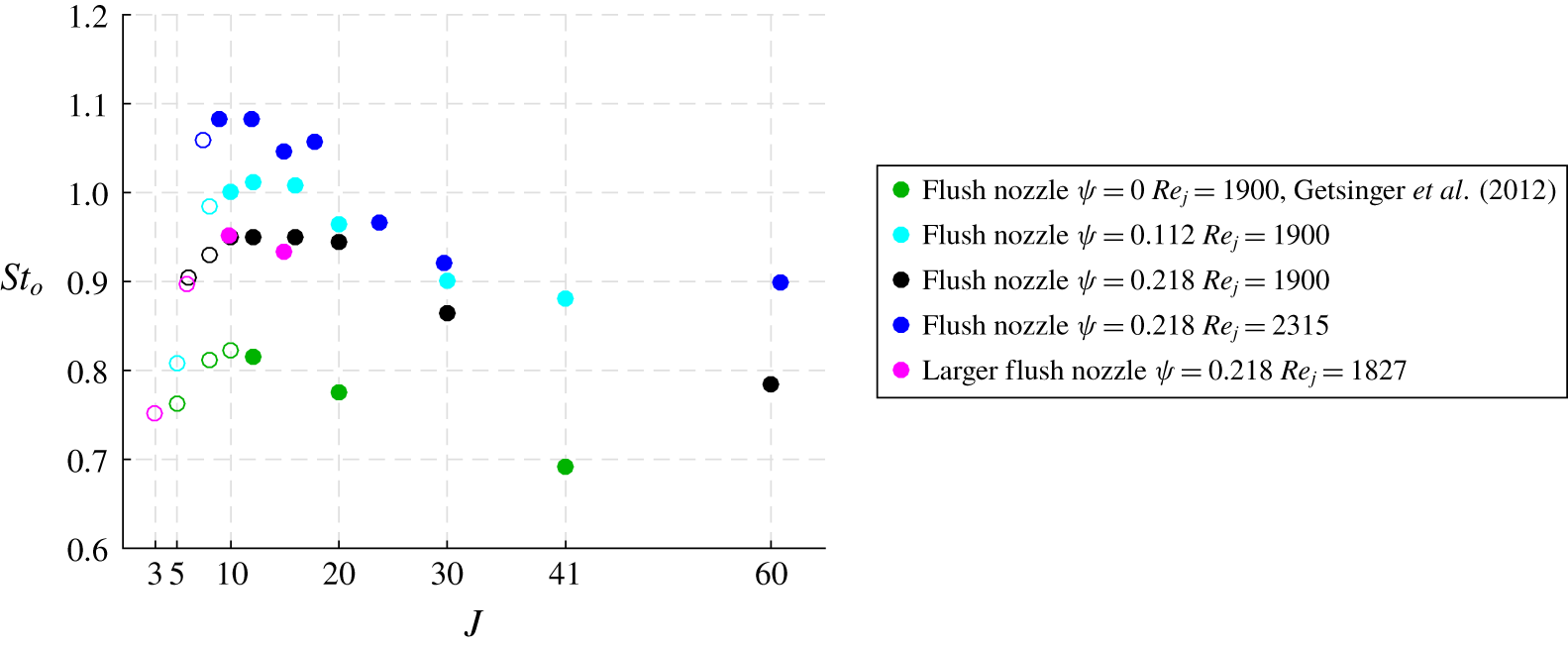
 $J$ were consistent with prior equidensity flush nozzle-injected JICF results in the absence of acetone (Megerian et al. Reference Megerian, Davitian, Alves and Karagozian2007). This is shown in figure 4 for various equidensity flow conditions, with different
 $Re_{j}$ values, gas constituents and two different nozzle diameters. For a fixed
 $Re_{j}$ and acetone concentration, as
 $J$ was reduced from a large value by increasing the cross-flow velocity, frequency
 $f_{o}$ and hence
 $St_{o}$ values from hot-wire-based spectra corresponding to convectively unstable flow always increased before reaching a peak at
 $J\approx J_{cr}$, and then decreased after the transition to global instability for
 $J<J_{cr}$. Figure 4 demonstrates a minimal influence of jet diameter for the same Reynolds number (e.g. comparing black and purple symbols), but a somewhat larger influence of
 $Re_{j}$ and
 $\unicode[STIX]{x1D713}$ on
 $J_{cr}$ (e.g. comparing green and dark blue symbols). Increasing the mole fraction of acetone appeared to reduce the value of
 $J_{cr}$, seen as the
 $J$ value at which the closed or filled symbols became open ones for a given set of conditions in figure 4. For a given
 $S$ and
 $Re_{j}$, a smaller
 $J_{cr}$ corresponded to an increase in the cross-flow velocity
 $U_{\infty }$ required to create transition to absolute instability. Increasing acetone concentrations also caused an increase in
 $f_{o}$ and hence in
 $St_{o}$, consistent with spectral contour plots (figure 3).
Variation in Strouhal number  $St_{o}$ for the fundamental USL mode based on jet diameter and mean jet velocity
 $U_{j}$ as a function of
 $J$ for the equidensity flush nozzle- and larger flush nozzle-injected JICF. Data are shown for
 $Re_{j}$ and acetone mole fractions
 $\unicode[STIX]{x1D713}$. Filled and open symbols represent the hot-wire-determined convectively and globally unstable USL, respectively.

The reduction in hot-wire-estimated  $J_{cr}$ with increasing concentrations of acetone in the jet fluid is recorded in table 1 for both equidensity and low-density flush nozzle-injected jets for experiments with a fixed
 $Re_{j}=1900$. Because jet density and Reynolds number were matched in these experiments for each
 $J$ value studied, and because the absolute viscosity of the mixture did vary among the cases for different concentrations of acetone, as determined via the Wilke formula (Bird et al. Reference Bird, Stewart and Lightfoot1960) and the Reichenberg method (Poling et al. Reference Poling, Prausnitz and O’Connell2001), the actual mean jet velocity
 $U_{j}$ at the exit plane necessarily differed slightly for the different acetone concentrations with otherwise constant bulk flow properties. The changes in
 $J_{cr}$ observed in figure 4 and in table 1 with acetone addition may be interpreted in the context of flow in the vicinity of the USL near the injection location, as will be shown.
3.2 Analogy to counter-current shear layer
Iyer & Mahesh (Reference Iyer and Mahesh2016) computationally demonstrate the phenomenological similarity in the USL instability transition for the flush nozzle-injected transverse jet to that for the CCSL based on the CCSL velocity ratio  $R_{1}$ in the centre plane, defined in (1.1). The present study explored this similarity based on numerous experimental datasets, using velocities extracted from PIV-only data for density ratios
 $S=1.00$,
 $0.70$,
 $0.55$ and
 $0.35$ (without the presence of acetone in the jet), taken from Getsinger (Reference Getsinger2012), and also using the PIV portion of simultaneous PLIF and PIV experiments at
 $S=1.00$ and
 $0.35$, many of which were taken from Shoji (Reference Shoji2017) and Gevorkyan et al. (Reference Gevorkyan, Shoji, Peng and Karagozian2018). Hence the acetone mole fractions in this comparison were relatively small,
 $\unicode[STIX]{x1D713}=0.112$.
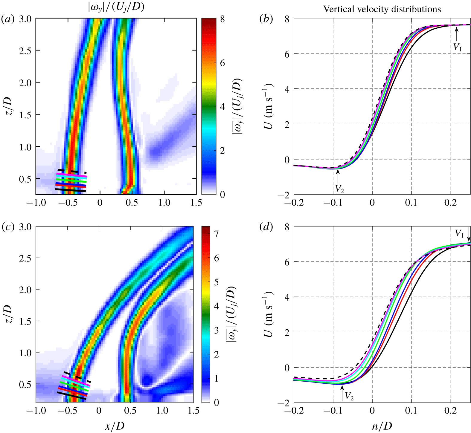
To extract the mixing layer (CCSL) velocity ratio  $R_{1}$ from PIV-based data, the same method as that used computationally in Iyer & Mahesh (Reference Iyer and Mahesh2016) was applied. First, the USL was defined by the magnitude of mean vorticity in the out-of-plane direction,
 $|\unicode[STIX]{x1D714}_{y}|$, as shown, for example, in figure 5(a) for the equidensity JICF with
 $J=20$. The normal direction to the USL,
 $n/D$, may be defined from the
 $|\unicode[STIX]{x1D714}_{y}|$ field, displayed using multiple lines close to the jet exit in figure 5(a). As done in the numerical studies (Iyer & Mahesh Reference Iyer and Mahesh2016), mean vertical velocity distributions then can be extracted at different locations
 $s/D$ just downstream of the jet exit, along the layer-normal direction
 $n/D$, as shown in figure 5(b). These velocity distributions were observed to have regions of both negative vertical velocity upstream of the USL centre and positive vertical velocity within the jet but outside of the USL, including a fairly uniform velocity profile near the jet centre, consistent with a nozzle-generated top-hat-like exit profile (examples of which, for a range of conditions, may be found in Gevorkyan et al. (Reference Gevorkyan, Shoji, Peng and Karagozian2018)). The near-field velocity profiles in figure 5(b) appeared quite analogous to those for a CCSL, and hence
 $V_{1}$ and
 $V_{2}$ could be extracted from such PIV-based data to evaluate the CCSL velocity ratio
 $R_{1}$ via (1.1). More details on the method of estimation of
 $R_{1}$ for the JICF may be found in Iyer & Mahesh (Reference Iyer and Mahesh2016). In the present experiments, the region upstream of the layer for which negative (vertically downward) flow occurred extended to distances in the negative layer-normal direction that depended on
 $J$. This negative flow region extended to approximately
 $n/D\approxeq -0.5$ for higher
 $J$ values such as
 $J=41$, but for lower
 $J$ values such as
 $J=5$, this region extended further, to
 $n/D\approxeq -2.0$.
(a,c) Normalized magnitude of vorticity in the out-of-plane direction,  $|\unicode[STIX]{x1D714}_{y}|$, for
 $J=20$ and
 $J=5$, respectively. (b,d) Vertical mean jet velocity distributions in the USL trajectory-normal direction,
 $n/D$, at variable trajectory locations,
 $s/D$, corresponding to
 $J=20$ and
 $J=5$, respectively, with the same line colours as in parts (a,c). Flow conditions correspond to the equidensity, nozzle-injected JICF with
 $Re_{j}=1900$ and
 $\unicode[STIX]{x1D713}=0.112$.

Data points show  $R_{1}$ versus
 $J$ for the JICF at different density ratios
 $S$ for a fixed
 $Re_{j}=1900$. Dashed lines corresponding to the colour of data points represent the theoretical velocity ratio,
 $R_{1,cr(th)}$, for the 2-D CCSL, while the grey region represents the range of experimentally observed values,
 $R_{1,cr(ex)}$. Circles represent
 $R_{1}$ values extracted from PIV-only experiments, while triangle symbols are based on data from simultaneous PLIF/PIV experiments with acetone at
 $\unicode[STIX]{x1D713}\approx 0.112$. Filled and open symbols represent convectively and absolutely/globally unstable conditions, respectively, determined via hot-wire anemometry. In (a), the purple squares represent
 $R_{1}$ determined from equidensity DNS by Iyer & Mahesh (Reference Iyer and Mahesh2016) at
 $Re_{j}=2000$.

Resultant  $R_{1}$ values for a range of experimental conditions with the flush nozzle are shown in figure 6(a) for the equidensity JICF and in figure 6(b–d) for the low-density JICF at density ratios
 $S$ equal to 0.70, 0.55 and 0.35, respectively. Filled and open symbols represent convectively and absolutely/globally unstable transverse jet USL conditions, respectively, determined experimentally via hot-wire-measured spectral characteristics such as those shown in figure 3. In addition, for most of the cases in figure 6(a–d), separate PIV-based proper orthogonal decomposition (POD) mode coefficient plots were examined to verify consistency with AU shear layer identification. As described in detail in Meyer, Pedersen & Özcan (Reference Meyer, Pedersen and Özcan2007) and Gevorkyan et al. (Reference Gevorkyan, Shoji, Peng and Karagozian2018), using snapshot POD analysis of the PIV-based jet centre plane data, plots of the POD coefficients of the first and second modes become circular when there is a periodic travelling wave flow structure consistent with an absolutely unstable USL. Such behaviour in the PIV-based experiments was used to verify consistency with the stability condition for the USL identified via hot-wire anemometry and indicated by the open circles in figure 6. The dashed lines in each panel indicate the established (theoretical) 2-D CCSL velocity ratio,
 $R_{1,cr(th)}$, for transition from a CU to AU shear layer for the given density ratio. These values are predicted by inviscid linear stability theory for the planar CCSL with
 $S=1$ from Huerre & Monkewitz (Reference Huerre and Monkewitz1985). For
 $S<1$, theoretical values of
 $R_{1,cr(th)}$ were extracted from the study by Pavithran & Redekopp (Reference Pavithran and Redekopp1989) for the CCSL, although it is noted that use of the Crocco–Busemann relation to compute density profiles can be inaccurate in representing the near field and thus in prediction of stability characteristics for light and hot jets (Coenen & Sevilla Reference Coenen and Sevilla2012). For all cases in figure 6, dashed lines theoretically distinguish convectively unstable conditions (
 $R_{1}<R_{1,cr}$) from absolutely unstable conditions (
 $R_{1}>R_{1,cr}$) for the CCSL. The transition from filled to open symbols in the panels enables estimation of the experimentally determined value or range of values for the critical velocity ratio,
 $R_{1,cr(ex)}$, indicated by the shaded regions in figure 6.
For the equidensity JICF without acetone in figure 6(a) (circles), corresponding to PIV-only experiments from which  $V_{1}$ and
 $V_{2}$ were extracted, AU conditions occurred when
 $J\lesssim 10$ according to hot-wire measurements. The corresponding value of
 $R_{1}$ at this AU transition was approximately 1.24, below the theoretical critical value,
 $R_{1,cr(th)}=1.32$. While there was a quantitative difference in the critical value of
 $R_{1}$, as one might expect for comparisons of a round, deflected shear layer with an idealized planar shear layer separated by infinite flow regions, the trends in figure 6(a) were consistent with the concept of the CCSL. That is, lower
 $J$ values producing absolute instability in the transverse jet corresponded to larger
 $R_{1}$ values, exceeding a critical value and thus being consistent with a self-excited CCSL. Hot-wire-determined convectively unstable conditions, with filled symbols in figure 6(a), similarly corresponded to
 $R_{1}<R_{1,cr(ex)}\approx 1.24$. These trends were also consistent with the DNS results for two different velocity ratios computed by Iyer & Mahesh (Reference Iyer and Mahesh2016), shown for reference in figure 6(a). These two computed data points for
 $R_{1}$ not only straddled the experimentally estimated value
 $R_{1,cr(ex)}\approx 1.24$, but also were consistent with the trends in the range of values shown by the experimental data points (circles, in the absence of acetone).
For the equidensity experiments with acetone present,  $V_{1}$ and
 $V_{2}$ extracted from the PIV portion of simultaneous PLIF and PIV measurements showed small yet systematic reductions in
 $V_{1}$ and less-negative values of
 $V_{2}$ as compared with extracted values in PIV-only experiments at the same
 $J$ and
 $Re_{j}$. These changes are reflected in the altered values of
 $R_{1}$ shown by the triangle symbols in figure 6(a), where the critical condition changed to
 $J_{cr}\lesssim 8$, with
 $R_{1,cr(ex)}\approx 1.23$. The differing
 $J_{cr}$ values associated with USL transition with and without acetone in figure 6(a) appeared to be associated with the slightly altered USL CCSL-like velocity distributions and the resulting small differences in the values of
 $V_{1}$ and
 $V_{2}$ close to the jet’s exit, thus producing a slightly different
 $R_{1}$. These differences in the velocity distributions resulted from small differences in the mean exit velocity
 $U_{j}$ that were required to match both
 $Re_{j}$ and
 $S$ for a given
 $J$ when the jet mixture contained acetone, with a different overall absolute viscosity
 $\unicode[STIX]{x1D707}_{j}$, as noted in § 3.1. Hence, while in both equidensity cases in figure 6(a) there was consistency in trends in the USL instability transition (from CU to AU, corresponding to increases in
 $R_{1}$), there was a small quantitative difference in
 $R_{1,cr}$ as well as in
 $J_{cr}$.
For the low-density JICF, trends in increasing  $R_{1}$ with a reduction in
 $J$ at matched
 $Re_{j}$ and
 $S$ were also consistent with the CCSL model, shown in figures 6(b), 6(c), and 6(d). The theoretical value of
 $R_{1,cr(th)}$ determined from Pavithran & Redekopp (Reference Pavithran and Redekopp1989) was somewhat larger than the PIV-based value of
 $R_{1,cr(ex)}$ for density ratio
 $S=0.70$ (figure 6b), though the band in which the transition from CU to AU took place (at
 $J_{cr}\lesssim 10$) was relatively wide in terms of estimating the critical
 $R_{1}$ range. For
 $S=0.55$ (figure 6c), the theoretical value of
 $R_{1,cr(th)}$ was slightly higher than the band at which PIV-only experiments indicated a transition from convective to absolute instability. Consistent with findings in Getsinger et al. (Reference Getsinger, Hendrickson and Karagozian2012), the very-low-density conditions for
 $S=0.35$ in figure 6(d) generally showed absolutely unstable USL conditions for virtually all
 $J$ values explored. An exception for the case with acetone present occurred at
 $J=41$, where the spectra were not quite the same as those associated with absolute instability, with a small degree of tonal interference. This condition for
 $J=41$ and
 $S=0.35$, which may have been marginally convectively unstable, produced CCSL velocity profiles corresponding to
 $R_{1}\approx 1.065$, well below that of the theoretical critical value of
 $R_{1,cr(th)}=1.12$ for this density ratio. We note that in Getsinger et al. (Reference Getsinger, Hendrickson and Karagozian2012) hot-wire measurements indicated that either
 $J<10$ or
 $S<0.40$ produced an absolutely/globally unstable USL, but data in figure 6(d) suggested that a
 $J$ value greater than
 $41$ at
 $S=0.35$ in the presence of acetone, or potentially greater than
 $J=52$ without acetone, could produce a convectively unstable USL, although such conditions were not attainable in the present experiments. Overall, then, there was general consistency between JICF shear layer transition and transition in a CCSL model from convective to absolute instability, even though the critical values of
 $R_{1}$ were typically smaller in the experiments than from the inviscid 2-D CCSL analysis. These findings suggest that the mechanism by which the JICF USL transition takes place, at least for the flush nozzle, could relate to the strengthening local counter-flow occurring at the jet exit.
It should be noted that the CCSL model here also provided some evidence for a mechanism for the development of the self-sustained global instability in the jet’s USL. Huerre & Monkewitz (Reference Huerre and Monkewitz1990) note that, as a flow transitions from convective to absolute instability, a ‘zone of local absolute instability’ forms. As the zone grows beyond a critical size, the system can become globally unstable, with a Hopf bifurcation to a self-sustained global mode. Huerre and Monkewitz note that the existence of this region of local absolute instability is a necessary though not sufficient condition for the existence of an amplified global mode. Evidence of global instability in the flush nozzle-injected transverse jet for a small enough  $J$ value, including evidence of a Hopf bifurcation (Davitian et al. Reference Davitian, Getsinger, Hendrickson and Karagozian2010; Regan & Mahesh Reference Regan and Mahesh2017), has already been documented both experimentally and computationally. The region of negative flow upstream of injection for the transverse jet, found here to grow in the negative
 $n/D$ direction as cross-flow velocity was increased (e.g. as in figure 5), could indeed represent this growing ‘zone of absolute instability’, providing additional evidence for transition to a global mode. This phenomenon appeared to occur even for the somewhat thick CCSLs created by this nozzle, as will be discussed below.
Additional features of the CCSL for which experimental data from the round JICF may be compared with 2-D theory include the Strouhal number associated with the fundamental shear layer instability but where the length scale of interest is the momentum thickness of the local near-field CCSL shown in figure 5. The linear stability theory of Huerre & Monkewitz (Reference Huerre and Monkewitz1985) for the equidensity 2-D CCSL suggests that the critical velocity ratio  $R_{1,cr}=1.315$ corresponds to a non-dimensional frequency of 0.192, which may be written in terms of a momentum-thickness-based Strouhal number
 $St_{\unicode[STIX]{x1D703}}\equiv f_{o}\unicode[STIX]{x1D703}_{o}/2\bar{V}=0.0153$, where the average velocity in the CCSL takes the form
 $\bar{V}\equiv \frac{1}{2}(V_{1}+V_{2})$. For the 2-D CCSL in figure 5(b), the momentum thickness in the near-field region of the layer may be approximated as
 $$\begin{eqnarray}\displaystyle \unicode[STIX]{x1D703}_{CCSL}=\int _{n_{V_{2}}}^{n_{V_{1}}}\frac{u(n)-V_{2}}{V_{1}-V_{2}}\left(1-\frac{u(n)-V_{2}}{V_{1}-V_{2}}\right)\,\text{d}n, & & \displaystyle\end{eqnarray}$$
where the limits of integration represent locations in the layer-normal direction at which the velocities reach the values of  $V_{1}$ and
 $V_{2}$. Strykowski & Niccum (Reference Strykowski and Niccum1991) compare an experimentally determined Strouhal number with the theoretical value of Huerre & Monkewitz (Reference Huerre and Monkewitz1985), but alter the limits of integration for (3.1) so that the lower limit is chosen to minimize uncertainties caused by very low velocities in the vicinity of the negative counter-flow. That lower limit
 $n_{L}$ corresponds to the location at which
 $(u-\bar{V})/(V_{1}-V_{2})=-0.4$. This produces a momentum thickness designated here as
 $\unicode[STIX]{x1D703}_{n_{L}}$. On this basis, the Strouhal number extracted from the Strykowski & Niccum (Reference Strykowski and Niccum1991) experiments at
 $R_{1}=1.4$ (above the critical limit) is
 $St_{\unicode[STIX]{x1D703}_{n_{L}}}=0.0185$. At a velocity ratio below the critical limit for the transition to absolute instability for the CCSL, at
 $R_{1}=1$, Strykowski & Niccum (Reference Strykowski and Niccum1991) observe that
 $St_{\unicode[STIX]{x1D703}_{n_{L}}}=0.012$, in agreement with the Strouhal number associated with the free jet shear layer by Hussain & Zaman (Reference Hussain and Zaman1978). Hussain & Zaman (Reference Hussain and Zaman1978) note the prevalence of a ‘shear layer mode’ at which vortex pairing has occurred, hence is associated with the subharmonic mode for the free jet, downstream of the spatial locations at which the authors observe tonal interference by a hot-wire probe producing frequency shifting of the fundamental mode; such subharmonic modes were seen for the transverse jet at higher momentum flux ratios, e.g. in figures 3(a–c).
In the present experiments for the JICF, one can make quantitative comparisons with the theoretical 2-D CCSL-based Strouhal numbers by evaluating relevant CCSL momentum thicknesses, either based on the definition in (3.1) for  $\unicode[STIX]{x1D703}_{CCSL}$ or based on
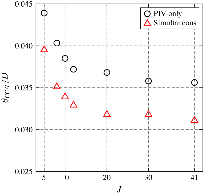
 $\unicode[STIX]{x1D703}_{n_{L}}$. Figure 7 shows the variations in momentum thickness
 $\unicode[STIX]{x1D703}_{CCSL}$ with
 $J$ for the equidensity JICF at
 $Re_{j}=1900$. The aforementioned differences in velocity magnitudes
 $V_{1}$ and
 $V_{2}$ with and without acetone, resulting from the effects of acetone on absolute viscosity and thus on the mean jet velocity
 $U_{j}$ and cross-flow velocity
 $U_{\infty }$ required to match
 $Re_{j}$ and
 $S$ for a given
 $J$, affected the CCSL velocity profiles and hence the momentum thicknesses. With the addition of acetone at the mole fraction shown for simultaneous PLIF and PIV,
 $\unicode[STIX]{x1D713}\approx 0.112$, figure 7 showed a reduction in non-dimensional momentum thickness
 $\unicode[STIX]{x1D703}_{CCSL}/D$ of approximately 17 % for the range of
 $J$ values shown. Corresponding values of
 $\unicode[STIX]{x1D703}_{nL}/D$ showed a similar reduction.
Variation in momentum thickness  $\unicode[STIX]{x1D703}_{CCSL}$ (scaled by
 $D$) for the local CCSL as a function of
 $J$ for the equidensity JICF at
 $Re_{j}=1900$. Results for data extracted from PIV-only experiments, without acetone, and simultaneous PLIF/PIV experiments, with acetone present at
 $\unicode[STIX]{x1D713}\approx 0.112$, are shown.

These differences in non-dimensional momentum thickness with and without acetone provided additional insights into the possible reasons for observed differences in the values of the critical CCSL velocity ratio  $R_{1}$ for the equidensity cases with and without acetone shown in figure 6(a). One would expect that the quantitative nature of the instabilities should be the same, based on the flow field’s dependence on non-dimensional parameters
 $J$,
 $Re$ and
 $S$ for a given transverse jet condition. The differences in the USL and the instabilities with and without acetone for the same values of these non-dimensional parameters suggested that an additional non-dimensional parameter could be relevant to the nature of the instabilities, per non-dimensional analysis. This non-dimensional parameter appeared to be the ratio of the jet-to-cross-flow absolute viscosities,
 $\unicode[STIX]{x1D707}_{j}/\unicode[STIX]{x1D707}_{\infty }$, causing the scaled CCSL momentum thickness
 $\unicode[STIX]{x1D703}/D$ to be dependent on the presence of acetone, as shown in figure 7. This issue will be discussed further below.
It is noted that the relatively large momentum thicknesses in figure 7, for example, producing  $D/\unicode[STIX]{x1D703}_{CCSL}$ values as large as 32 for
 $J=41$ with acetone and as small as 23 for
 $J=5$ without acetone, were thicker than those typically considered to be thin enough so that shear layer curvature effects may be considered negligible (
 $D/\unicode[STIX]{x1D703}$ of the order of 50, per Huerre & Monkewitz (Reference Huerre and Monkewitz1985), and larger, of the order of 230, by Strykowski & Niccum (Reference Strykowski and Niccum1991)). The momentum thickness can impact application of planar CCSL inviscid instability theory in predicting fundamental instability frequencies, as noted by Strykowski & Niccum (Reference Strykowski and Niccum1991). For example, LSA for the planar CCSL (Jendoubi & Strykowski Reference Jendoubi and Strykowski1994) suggests that the critical value of
 $R_{1,cr}$ can change with more significant reductions in
 $D/\unicode[STIX]{x1D703}$, which in the case of the JICF would correspond to lower
 $J$ conditions, e.g.
 $J=5$. Yet the actual experimental values of
 $R_{1}$ for this range of momentum thicknesses and
 $J$ values shown in figure 6(a) were very close to DNS-based results (Iyer & Mahesh Reference Iyer and Mahesh2016) for similar flow conditions. For the strongly deflected jet in cross-flow, one would expect curvature effects in the round jet as well as the increasingly non-parallel flow along the curved USL to be inconsistent with an idealized 2-D CCSL, as also noted by Iyer & Mahesh (Reference Iyer and Mahesh2016). Nevertheless, it is remarkable that the quantitative prediction of transition to JICF global instability was generally close to values of
 $R_{1,cr(th)}$ predicted by inviscid 2-D LSA, both with and without the presence of acetone, indicated in figure 6. Hence it was of interest to utilize momentum thickness in comparing the present instability frequencies with established ranges of Strouhal number for the planar CCSL.
Variation in Strouhal number based on momentum thickness,  $St_{\unicode[STIX]{x1D703}_{CCSL}}\equiv f_{o}\unicode[STIX]{x1D703}_{CCSL}/2\bar{V}$, as a function of
 $J$ for the equidensity JICF case at
 $Re_{j}=1900$. Results for data extracted from PIV-only experiments, without acetone, and simultaneous PLIF/PIV experiments, with acetone present at
 $\unicode[STIX]{x1D713}\approx 0.112$, are shown.

Figure 8 shows the variation in Strouhal number based on  $\unicode[STIX]{x1D703}_{CCSL}$ derived from PIV-only and simultaneous PLIF/PIV experimental datasets for the equidensity JICF at
 $Re_{j}=1900$. Remarkably, for a Strouhal number based on CCSL-based momentum thickness scaling rather than diameter
 $D$, and based on twice the average velocity in the CCSL,
 $2\bar{V}$ rather than average jet velocity
 $U_{j}$ (which does not capture the effect of the local negative flow upstream of the jet), there was a generally good collapse of the data for cases with and without acetone in the jet fluid. An exception was seen in the case of the very low momentum flux ratio jet, with
 $J=5$, which as noted previously had the thickest and most deflected USL. It is remarkable that
 $St_{\unicode[STIX]{x1D703}}$ values with and without acetone at a given
 $J$ value collapsed onto one another for most cases in figure 8, in contrast to the differing Strouhal numbers based on diameter and mean jet velocity in figure 4, shown by data points indicated in green and cyan. The results in figure 8 thus provided further evidence for the importance of the non-dimensional parameter
 $\unicode[STIX]{x1D703}/D$, related to differences in jet fluid viscosity, and the relevance of the CCSL model in interpreting JICF shear layer instability transition. For the clearly convectively unstable flows at
 $J=41$, for example,
 $St_{\unicode[STIX]{x1D703}}$ was of the order of 0.023–0.024, corresponding to
 $St_{o}$ values of approximately 0.7 without acetone and approximately 0.9 with an acetone mole fraction
 $\unicode[STIX]{x1D713}=0.112$ (figure 4). These frequencies corresponded to the fundamental mode for the convectively unstable JICF with spectral characteristics as in figure 3(a); the observed subharmonics thus had
 $St_{\unicode[STIX]{x1D703}}$ values of the order of 0.011–0.012. The
 $J=41$ condition here produced
 $R_{1}\approx 1.09$, below the experimentally observed critical condition for the CCSL,
 $R_{1,cr}\approx 1.24$. These measured Strouhal numbers associated with
 $R_{1}\approx 1.09$ were approximately twice as large as those observed for the free jet by Hussain & Zaman (Reference Hussain and Zaman1978) and Strykowski & Niccum (Reference Strykowski and Niccum1991) at
 $R_{1}=1.0$. As
 $J$ was reduced and the critical condition for transition to global instability approached in figure 8, the values of
 $St_{\unicode[STIX]{x1D703}}$ increased to the range of 0.03 (
 $J=10$) to 0.037 (
 $J=5$ with acetone), also approximately twice as large as established theory and experiments for the planar CCSL (Huerre & Monkewitz Reference Huerre and Monkewitz1985; Strykowski & Niccum Reference Strykowski and Niccum1991). The well-established trend for the CCSL, whereby Strouhal number increases rather abruptly as one approaches the critical condition (Strykowski & Niccum Reference Strykowski and Niccum1991), is consistent with observations in figure 8.
These differences in fundamental Strouhal number  $St_{\unicode[STIX]{x1D703}}$ between the present experiments and the established 2-D CCSL values were probably not so much the result of slightly different CCSL velocity ratios
 $R_{1}$ at transition as the relatively large CCSL momentum thickness at and beyond critical conditions, as noted previously. More importantly, Huerre & Monkewitz (Reference Huerre and Monkewitz1990) note that the frequency selection criterion for global instability depends on how the absolutely unstable frequency evolves spatially, which in turn depends on the development of the base flow for the flow field. The spatial development in a counter-current, planar mixing layer is typically much slower than the spatial development observed in a transverse jet, as indicated in earlier transverse jet stability studies (Alves et al. Reference Alves, Kelly and Karagozian2007, Reference Alves, Kelly and Karagozian2008), and the global frequency determination here is not a local feature of the flow, in contrast to the determination of the critical parameter (
 $R_{1,cr}$) for the onset of absolute instability. Hence in many respects one would not expect the JICF Strouhal numbers
 $St_{\unicode[STIX]{x1D703}}$ to correspond very closely to the established values for the planar CCSL.
4 Discussion and conclusions
This experimental study provides evidence that the phenomena associated with the USL instability transition for the flush nozzle-injected transverse jet can be understood in the context of transition in the CCSL instability. Consistent qualitative and quantitative trends in flow conditions creating convective versus absolute/global instability in the USL, and comparisons with established trends from planar LSA predictions (figure 6), speak to the importance of the degree of counter-flow just upstream of the jet exit. Further insights may be gleaned from noting that the region of negative flow forming upstream of injection for the transverse jet, measured here to grow in the negative  $n/D$ direction as cross-flow velocity was increased, could indeed represent a growing ‘zone of absolute instability’, based on
 $J$, a necessary requirement for transition of the instability to a global mode (Huerre & Monkewitz Reference Huerre and Monkewitz1990).
Alterations in the Strouhal number associated with the USL instabilities with a reduction in momentum flux ratio  $J$, while approaching the critical CCSL velocity ratio,
 $R_{1,cr}$, were also consistent with established trends observed for the CCSL, with a collapse of frequency data when Strouhal number was scaled in terms of momentum thickness. The
 $St_{\unicode[STIX]{x1D703}}$ values in the present study for a range of
 $J$ values were approximately twice as large as theoretical values for the equidensity 2-D CCSL (Huerre & Monkewitz Reference Huerre and Monkewitz1985; Strykowski & Niccum Reference Strykowski and Niccum1991). It is likely that an altered theoretical exploration of the CCSL, an LSA applied to a round jet shear layer with external counter-flow, could provide improved comparisons with the present experiments.
Interestingly, in the DNS for the flush nozzle-generated JICF by Iyer & Mahesh (Reference Iyer and Mahesh2016), the convectively unstable USL condition ( $J=16$) produces spectral characteristics in which a lower frequency, corresponding to
 $St_{o}=0.39$ (based on diameter), is initially observed to occur close to the jet exit, at a location
 $s/D=0.1$. This value is half that of the fundamental instability observed in experiments (Megerian et al. Reference Megerian, Davitian, Alves and Karagozian2007). But then a bit further along the shear layer, for
 $s/D\geqslant 1.0$, the same Strouhal number as in experiments is found to dominate the flow (
 $St_{o}=0.78$, as shown in figure 4). This observation could be attributed, as suggested by Iyer & Mahesh (Reference Iyer and Mahesh2016), to the very low amplitude of the initial spectral peak observed in the computations, below the noise floor for hot-wire measurements in the experiments. The dominance of the
 $St_{o}=0.78$ fundamental mode for that flow condition in the DNS, and consistency with experiments for that condition and for Strouhal numbers associated with global instability at
 $J=4$, suggests that the frequencies quantified in the present study could well be physically relevant to those predicted via DNS.
Ultimately, the general consistency between the degree of counter-flow required for CCSL transition and transition in the transverse jet’s USL enables new insights into the dynamical mechanisms associated with the JICF. Clearly, a more robust comparison of transverse jet USL instability transition with the concept of the CCSL requires that the theory represents more closely the actual round jet injected flush into a strengthening cross-flow (or at least counter-flow). Overall, however, even this simple comparison with the 2-D CCSL model provides information that can be used to control jet behaviour, for example, involving active alteration of the flow just upstream of injection to alter USL stability characteristics. This approach is the subject of ongoing studies involving control of this important flow field.
Acknowledgements
The authors wish to express their thanks to Professor L. Alves of the Universidade Federal Fluminense (UFF) for helpful discussions and insights in this study. This research has been supported by the National Science Foundation under grant CBET-1437014 and by the Air Force Office of Scientific Research under grant FA9550-15-1-0261.
Declaration of interests
The authors report no conflict of interest.