2. Linear stability analysis

In general, a dual layer contains four fluids and three interfaces. Although it is the simplest multilayer, it is still too complex to find analytical solutions, as pointed out by Mikaelian (Reference Mikaelian1985), who showed that analytical solutions could not be derived when the number of fluids is larger than three and the number of interfaces is larger than two. To solve this problem, we consider a simplified system that consists of two incompressible and initially irrotational fluids and three nearly planar interfaces with single-mode perturbations $\eta _1$, $\eta _2$ and $\eta _3$, in a vacuum, with gravitation $g$ (Guo et al. Reference Guo, Wang, Ye, Wu and Zhang2017; Liu et al. Reference Liu, Li, Yu, Fu, Wang, Wang and Ye2018b), as shown in figure 1, and which resembles the outer ablator layer and the middle push layer of an ICF capsule. Fluid with density $\rho _a$, velocity potential $\phi _a$ and thickness $h_a$ is overlapped on another fluid with density $\rho _b$, velocity potential $\phi _b$ and thickness $h_b$. The velocity potentials $\phi _a$ and $\phi _b$ satisfy

(2.1)\begin{equation} \nabla^{2}\phi=0. \end{equation}

Figure 1.

The configuration of the dual-layer system that consists of two incompressible and initially irrotational fluids and three nearly planar interfaces with perturbations $\eta _1$, $\eta _2$ and $\eta _3$, in a vacuum, with gravitation $g$. Fluid with density $\rho _a$, velocity potential $\phi _a$ and thickness $h_a$ is overlapped on another fluid with density $\rho _b$, velocity potential $\phi _b$ and thickness $h_b$.

To obtain a linear solution, the periodic small perturbation amplitudes set on the first interface ($a_1$), second interface ($a_2$) and third interface ($a_3$) are of the form

(2.2a–c)\begin{equation} \eta_1=a_1(t)\cos(kx),\quad \eta_2=a_2(t)\cos(kx),\quad \eta_3=a_3(t)\cos(kx). \end{equation}

The first (respectively third) interface is a free boundary located at $y=\eta _1+ h_a$ (respectively $y=\eta _3-h_b$), and the second interface is at $y=\eta _2$ with vertical velocity being continuous. Then the kinematic conditions on the boundaries are

(2.3)\begin{equation} \left.\begin{gathered} \frac{\partial\eta_1}{\partial t}+\frac{\partial\eta_1}{\partial x} \frac{\partial\phi_a}{\partial x}-\frac{\partial\phi_a}{\partial y}=0,\quad \textrm{at}\ y=\eta_1+h_a,\\ \frac{\partial\eta_2}{\partial t}+\frac{\partial\eta_2}{\partial x} \frac{\partial\phi_a}{\partial x}-\frac{\partial\phi_a}{\partial y}=0,\quad \textrm{at}\ y=\eta_2,\\ \frac{\partial\eta_3}{\partial t}+\frac{\partial\eta_3}{\partial x} \frac{\partial\phi_b}{\partial x}-\frac{\partial\phi_b}{\partial y}=0,\quad \textrm{at}\ y=\eta_3-h_b,\\ \frac{\partial\eta_2}{\partial t}+\frac{\partial\eta_2}{\partial x} \frac{\partial\phi_b}{\partial x}-\frac{\partial\phi_b}{\partial y}=0,\quad \textrm{at}\ y=\eta_2, \end{gathered}\right\} \end{equation}

and the conditions of the pressure equilibrium are

(2.4)\begin{equation} \left.\begin{gathered} \frac{\partial\phi_a}{\partial t}+\frac{(\boldsymbol{\nabla}\phi_a)^{2}}{2} +g\eta_1=0,\quad \textrm{at}\ y=\eta_1+h_a,\\ \frac{\partial\phi_b}{\partial t}+\frac{(\boldsymbol{\nabla}\phi_b)^{2}}{2} +g\eta_3=0,\quad \textrm{at}\ y=\eta_3-h_b,\\ \rho_a\left[\frac{\partial\phi_a}{\partial t} +\frac{(\boldsymbol{\nabla}\phi_a)^{2}}{2}+g\eta_2\right] =\rho_b\left[\frac{\partial\phi_b}{\partial t} +\frac{(\boldsymbol{\nabla}\phi_b)^{2}}{2}+g\eta_2\right], \quad \textrm{at}\ y=\eta_2. \end{gathered}\right\} \end{equation}

Combining the above equations, linearising the equations by neglecting the products $(\partial \eta /\partial x)(\partial \phi /\partial x)$ and terms $(\boldsymbol {\nabla }\phi )^{2}$, and replacing the acceleration $g$ by the product of the post-shock flow speed (${\rm \Delta} v$) and a Dirac delta function, the linear solutions for the amplitude growth rates of the first interface ($\dot {a}_1^{l}$), second interface ($\dot {a}_2^{l}$) and third interface ($\dot {a}_3^{l}$) induced by RMI can be obtained as

(2.5)\begin{align} \dot{a}_1^{l}&=\frac{k{\rm \Delta} v \, a_2(0)}{1-\alpha^{2}\beta^{2}+\alpha\xi_1(\beta^{2}-1)+\beta\xi_2(\alpha^{2}-1)} \{\epsilon_1(\beta\xi_2-1)+\xi_1(1-\beta\epsilon_3) \nonumber\\ &\quad +\alpha\beta(\epsilon_3-\xi_2)-A\xi_1[1-\alpha^{2}\beta^{2} -\alpha(\epsilon_1-\alpha\beta\epsilon_3)- \beta(\epsilon_3-\alpha\beta\epsilon_1)] \nonumber\\ &\quad +\alpha\beta[\epsilon_3(1-\alpha\xi_1)-\alpha\beta(\epsilon_1-\xi_1) -\xi_2(1-\alpha\epsilon_1)]\}, \end{align}

(2.6)\begin{align} \dot{a}_2^{l}&=\frac{k{\rm \Delta} v \, a_2(0)}{1-\alpha^{2}\beta^{2}+\alpha\xi_1(\beta^{2}-1)+\beta\xi_2(\alpha^{2}-1)} \{A[\alpha^{2}\beta^{2}-1+\alpha(\epsilon_1-\alpha\beta\epsilon_3) \nonumber\\ &\quad +\beta(\epsilon_3-\alpha\beta\epsilon_1)] -\alpha[\epsilon_1(1-\beta\xi_2)-\xi_1(1-\beta\epsilon_3) -\alpha\beta(\epsilon_3-\xi_2)] \nonumber\\ &\quad +\beta[\epsilon_3(1-\alpha\xi_1)-\alpha\beta(\epsilon_1-\xi_1) -\xi_2(1-\alpha\epsilon_1)]\}, \end{align}

(2.7)\begin{align} \dot{a}_3^{l}&=\frac{k{\rm \Delta} v\, a_2(0)}{1-\alpha^{2}\beta^{2}+\alpha\xi_1(\beta^{2}-1)+\beta\xi_2(\alpha^{2}-1)} \{\epsilon_3(1-\alpha\xi_1)-\alpha\beta(\epsilon_1-\xi_1)\nonumber\\ &\quad -\xi_2(1-\alpha\epsilon_1)-A\xi_2[1-\alpha^{2}\beta^{2} -\alpha(\epsilon_1-\alpha\beta\epsilon_3)- \beta(\epsilon_3-\alpha\beta\epsilon_1)] \nonumber\\ &\quad -\alpha\beta[\epsilon_1(1-\beta\xi_2)-\alpha\beta(\epsilon_3-\xi_2) -\xi_1(1-\beta\epsilon_3)] \}. \end{align}

Here $A=(\rho _b-\rho _a)/(\rho _b+\rho _a)$ is the Atwood number of the inner interface (i.e. the second interface), $\alpha =\mathrm {e}^{-kh_a}$, $\beta =\mathrm {e}^{-kh_b}$, $\xi _1=-2\alpha (1-\beta ^{2})A/[(1-\alpha ^{2}\beta ^{2})(1-A)]$, $\xi _2=2\beta (1-\alpha ^{2})A/[(1-\alpha ^{2}\beta ^{2})(1+A)]$, $\epsilon _1=a_1(0)/a_2(0)$ and $\epsilon _3=a_3(0)/a_2(0)$. When $kh_a\rightarrow \infty$ or (and) $kh_b\rightarrow \infty$, the linear solutions (2.5)–(2.7) reduce to being applicable to the single-layer (semi-infinite) RMI. We note that the linear solutions (2.5)–(2.7) do not consider the effect of reverberating waves on the interfacial instabilities, which will further complicate the analysis and will be discussed later.

To eliminate the 2-D feature of the reverberating waves and validate the linear solutions by experiments, we further simplify the configuration by assuming that the exterior interfaces (i.e. the first and third interfaces) are initially unperturbed, i.e. $\epsilon _1=0$ and $\epsilon _3=0$ (see figure 2b). Then the linear solutions for this system reduce to

(2.8a–c)\begin{equation} \dot{a}_1^{l}=\psi_1\dot{a}_2^{R},\quad \dot{a}_2^{l}=\psi_2\dot{a}_2^{R},\quad \dot{a}_3^{l}=\psi_3\dot{a}_2^{R}, \end{equation}

with

(2.9)\begin{equation} \left.\begin{gathered} \psi_1=\frac{\xi_1[1-A-\alpha^{2}\beta^{2}(1+A)] -2\alpha\beta\xi_2}{A[\alpha^{2}\beta^{2}-1-\alpha \xi_1(\beta^{2}-1)-\beta\xi_2(\alpha^{2}-1)]},\\ \psi_2=\frac{A(\alpha^{2}\beta^{2}-1)+\alpha\xi_1(1+\beta^{2}) -\beta\xi_2(1+\alpha^{2})}{A[\alpha^{2} \beta^{2}-1-\alpha\xi_1(\beta^{2}-1)-\beta\xi_2(\alpha^{2}-1)]},\\ \psi_3=\frac{2\alpha\beta\xi_1 -\xi_2[A+1+\alpha^{2}\beta^{2}(1-A)]}{A[\alpha^{2}\beta^{2}-1-\alpha \xi_1(\beta^{2}-1)-\beta\xi_2(\alpha^{2}-1)]}, \end{gathered}\right\} \end{equation}

and the Richtmyer growth rate (Richtmyer Reference Richtmyer1960) is

(2.10)\begin{equation} \dot{a}_2^{R}=Za_2(0)kA{\rm \Delta} v_2. \end{equation}

Here ${\rm \Delta} v_2$ is the jump speed of the second interface and the compression factor $Z=1-{\rm \Delta} v_2/v_{{TS}_1}$, with $v_{{TS}_1}$ the speed of the incident shock relative to the inner interface. If $A<0$, (2.10) is replaced by the Meyer–Blewett growth rate (Meyer & Blewett Reference Meyer and Blewett1972): $\dot {a}_2^{R}=(Z+1)a_2(0)kA{\rm \Delta} v_2/2$. Although the exterior interfaces are initially unperturbed, the layer-coupling effect imposes the growth rates related to the inner interface on the exterior interfaces (see (2.8a–c)). Further, $\psi _2$ in (2.9) quantifies the layer-coupling effect on the inner interface. We note that the simplified configuration keeps all the essential physics such as the layer coupling, but greatly reduces the difficulty in experiment implementation and the non-uniformity of the flow between the layers.

Figure 2.

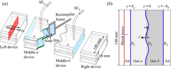
Schematics of (a) the soap-film interface generation and (b) the initial configuration. Here II$_1$, II$_2$ and II$_3$ denote the initial first, second and third interfaces, respectively.

3. Experimental method

Shock-tube experiments on such a simplified dual layer are performed in a horizontal shock tube with a $140~\textrm {mm} \times 10~\textrm {mm}$ cross-sectional area to validate the simplified linear solutions (2.8a–c)–(2.10). First, the soap-film technique is utilised to generate shape-controllable and discontinuous quasi-2-D interfaces on the two sides of the middle-$a$ device and the left side of the middle-$b$ device, as shown in figure 2(a), mainly eliminating the additional short-wavelength perturbations, diffusion layer and three-dimensionality of the initial interfaces (Liu et al. Reference Liu, Liang, Ding, Liu and Luo2018a; Liang et al. Reference Liang, Zhai, Ding and Luo2019). Then the air in the middle-$a$ device and middle-$b$ device is replaced by different volumes of SF$_6$. Finally, the left, middle-$a$, middle-$b$ and right devices (see figure 2a) are combined and inserted in the shock tube, and the shock-tube experiments are conducted. Because the density of pure SF$_6$ is about five times that of air, it is reasonable to approximate the theoretical configuration with present experiments, although the dual layer is formed in the air, not a vacuum, in the experiments.

In the Cartesian coordinate system (indicated in figure 2b), the initial amplitude imposed on the inner interface is $a_{2}(0)=2.0$  mm, and the wavenumber is $k=104.7$  m$^{-1}$. The physical parameters of the dual-layer (i.e. cases D-L$\#$LH and D-L$\#$HL; ‘D-L’ represents dual layer; ‘L’, light; and ‘H’, heavy), single-layer (i.e. cases S-L$\#$LH and S-L$\#$HL; ‘S-L’ represents single layer) and semi-infinite (i.e. cases S-I$\#$LH and S-I$\#$HL; ‘S-I’ represents semi-infinite) interfaces are listed in table 1. Illuminated by a continuous light source (CEL-HXF300, maximum power output 249  W), the flow field is monitored by high-speed Schlieren photography. The frame rate of the high-speed video camera (FASTCAM SA5, Photron Ltd, with a sensor of 1024 pixels $\times$ 1024 pixels) is 60 000 frames per second with a shutter time of 1  $\mathrm {\mu }$s. The spatial resolution of the Schlieren images is 0.4 mm  pixel$^{-1}$. In this study, the waves’ displacements and speeds, and the amplitudes of the three interfaces, are measured from the Schlieren images. The measurement accuracies for the waves’ speeds are 1 m  s$^{-1}$, and for the waves’ displacements and the interface amplitudes are 0.4  mm. The ambient pressure and temperature are 101.3  kPa and $299.5 \pm 1.0$  K, respectively. For each case, at least three experimental runs are performed, and the maximum variances from the mean for the inner interface amplitudes among diverse experimental runs are within  3 %.

Table 1.

Physical parameters of gas layers: $h_a$ and $h_b$ are layer thicknesses; $M$ denotes the incident shock Mach number; $mf_a$ ($mf_b$) is the mass fraction of SF$_6$ in gas $a$ (gas $b$); $A$ denotes the Atwood number of the second interface; ${\rm \Delta} v_1$ and ${\rm \Delta} v_2$ denote the jump speed of the first and second interface, respectively; $v_{{TS}_1}$ and $v_{{TS}_2}$ denote the speed of the transmitted shock ${\rm TS}_1$ and ${\rm TS}_2$, respectively; $|\dot {\zeta _2}|$ denotes the dimensionless amplitude growth rate of the second interface measured from experiments; and $\psi _1$, $\psi _2$ and $\psi _3$ are dimensionless parameters calculated with (2.9). The units of thickness and speed are mm and m s$^{-1}$, respectively.

4. One-dimensional motions of waves and interfaces

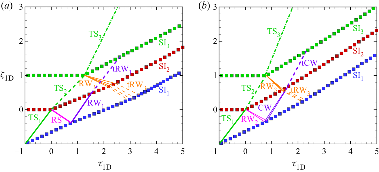
Owing to the different acoustic impedances of the various fluids in a dual layer, the reverberating waves inside the layers are multifarious. Based on the one-dimensional (1-D) gas dynamics theory (Drake Reference Drake2018; Liang & Luo Reference Liang and Luo2021), 1-D dimensionless $t$–$y$ diagrams of the three interfaces and reverberating waves in cases D-L$\#$LH and D-L$\#$HL are shown in figures 3(a) and 3(b), respectively. Note that only significant waves for interface evolution are presented in the figures. The moment when the initial inner interface (II$_2$) is first shocked is defined as $t=0$. Time is scaled as $\tau _{{1D}}=tv_{{TS_1}}/h_a$. Displacements of interfaces and waves are scaled as $\zeta _{{1D}}=y/h_a$.

Figure 3.

One-dimensional dimensionless $t$–$y$ diagrams of a shocked dual layer in the (a)  D-L$\#$LH case and (b)  D-L$\#$HL case. TS, transmitted shock; RS, reflected shock; RW, rarefaction waves; tRW, transmitted rarefaction waves; CW, compression waves; tCW, transmitted compression waves; SI$_1$, SI$_2$ and SI$_3$, shocked first, second and third interface. Blue, red and green symbols represent the first, second and third interfaces’ trajectories. Lines represent the waves’ trajectories.

In the D-L$\#$LH case, after the incident shock first impacts the initial first interface (II$_1$), a transmitted shock (TS$_1$) is refracted inside gas $a$ and moves towards the initial second interface (II$_2$). Second, after the TS$_1$ impacts the II$_2$, a transmitted shock (TS$_2$) is refracted inside gas $b$, and a reflected shock (RS) is generated and moves backwards, since the inner interface is a fast/slow one relative to the motion of TS$_1$. Third, after the RS impacts the shocked first interface (SI$_1$), the SI$_1$ decelerates, and rarefaction waves (RW$_1$) are reflected inside gas $a$, since the first interface is a slow/fast one relative to the motion of RS. Moreover, after the TS$_2$ impacts the initial third interface (II$_3$), a transmitted shock (TS$_3$) is refracted outside the layers, and rarefaction waves (RW$_3$) are reflected inside gas $b$, since the third interface is also a slow/fast one relative to the motion of TS$_2$. Fourth, the RW$_1$ impacts the shocked inner interface (SI$_2$), decelerating the SI$_2$ and refracting transmitted rarefaction waves (tRW$_1$) into gas $b$. Subsequently, the RW$_3$ impacts the SI$_2$, accelerating the SI$_2$ and refracting transmitted rarefaction waves (tRW$_3$) into gas $a$. Since the strength of the RW$_3$ is much larger than that of the RW$_1$, the final velocity of SI$_2$ is larger than the initial velocity jump induced by the TS$_1$. Fifth, the tRW$_1$ impacts and decelerates the shocked third interface (SI$_3$), and the tRW$_3$ impacts and accelerates the SI$_1$. Finally, all waves refract outside the dual layer, and the three interfaces move at the same speed.

In the D-L$\#$HL case, after the TS$_1$ impacts the II$_2$, rarefaction waves (RW$_2$) are reflected inside gas $a$, since the inner interface is a slow/fast one relative to the motion of TS$_1$. Then, after the RW$_2$ impacts the SI$_1$, the SI$_1$ accelerates, and compression waves (CW) are reflected inside gas $a$, since the first interface is a slow/fast one relative to the motion of RW$_2$. Later, the CW impacts the SI$_2$, accelerating the SI$_2$ and refracting transmitted compression waves (tCW) into gas $b$. In addition, since the density gradient at the third interface is lower in the D-L$\#$HL case on comparing with the D-L$\#$LH case, the RW$_3$ in the D-L$\#$LH case is stronger than that in the D-L$\#$HL case.

5. Two-dimensional hydrodynamic instabilities

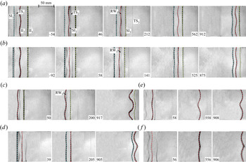
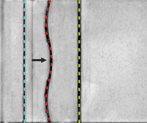
Schlieren images of the shock-induced evolutions of the dual-layer (three interfaces), single-layer (two interfaces) and semi-infinite (one interface) interfaces are shown in figure 4(a–f). In general, the waves in the 2-D case are similar to the 1-D counterparts and, therefore, we shall take the D-L$\#$LH case as an example to discuss only the deformations of the three interfaces. First, after the TS$_1$ impacts the II$_2$ (46  $\mathrm {\mu }$s), the rippled TS$_2$ is refracted inside gas $b$. Meanwhile, the perturbation on the inner interface grows gradually. Second, after the rippled TS$_2$ impacts the II$_3$, the II$_3$ is slightly deformed and the RW$_3$ impacts and accelerates the evolving SI$_2$ (212  $\mathrm {\mu }$s). Third, after the RW$_3$ impacts the perturbed SI$_2$, rippled reverberating waves inside the two layers impact the nearly planar SI$_1$ and SI$_3$. Last, the three interfaces evolve with the same phase, and one can find that the largest perturbation is on the inner interface, and the smallest perturbation is on the third interface (912  $\mathrm {\mu }$s).

Figure 4.

Schlieren images of shocked-layer evolutions in cases (a)  D-L$\#$LH, (b)  D-L$\#$HL, (c)  S-L$\#$LH, (d)  S-L$\#$HL, (e)  S-I$\#$LH and (f)  S-I$\#$HL. The first, second and third interfaces are marked with blue, red and green dashed lines, respectively. Numbers denote time in $\mathrm {\mu }$s.

The time-varying dimensionless amplitudes of the inner interface in three $A>0$ cases (i.e. cases D-L$\#$LH, S-L$\#$LH and S-I$\#$LH) and three $A<0$ cases (i.e. cases D-L$\#$HL, S-L$\#$HL and S-I$\#$HL) are measured and shown in figures 5(a) and 5(b), respectively. Time is scaled as $\tau _2=k|\dot {a}_2^{l}|t$, and amplitude is scaled as $\zeta _2=k(a_2-Za_2(0))$. Here we calculate $\psi _1$, $\psi _2$ and $\psi _3$ using (2.9) by considering the shock compression on the initial layer thicknesses, i.e. $\alpha =\exp ({-kZ_{a}h_a})$ and $\beta =\exp ({-kZ_{b}h_b})$ with $Z_{a}=1-{\rm \Delta} v_1/v_{{TS}_1}$ and $Z_{b}=1-{\rm \Delta} v_2/v_{{TS}_2}$, where ${\rm \Delta} v_1$ is the velocity jump at the first interface, and $v_\mathrm {TS_2}$ is the velocity of TS$_2$, respectively, as listed in table 1. The dimensionless amplitude growth rate ($|\dot {\zeta _2}|$) of the inner interface is obtained by linearly fitting the $\zeta _2$ before the RW$_3$ impacts the inner interface, as listed in table 1. Before the RW$_3$ impacts the two interfaces (as marked with vertical dash-dotted lines), the good agreement between the $\zeta _2$ with the predictions of linear solutions (as marked with black dashed lines with a slope of 1 for $A>0$ cases or $-1$ for $A<0$ cases) validates the established linear solutions. Likewise, the agreement between $\psi _2$ with $|\dot {\zeta _2}|$ in all cases also validates the linear solutions (see table 1). In addition, the $\psi _2$ in the $A>0$ cases is larger than in the corresponding $A<0$ cases. On the one hand, the phase reversal involved in the $A<0$ cases enlarges the difference of the inner interface amplitude between $A>0$ conditions and $A<0$ conditions. On the other hand, the RW$_3$ is weaker in the $A<0$ cases and induces less additional vorticity deposition on the inner interface (the effect of RW$_3$ will be discussed in detail later).

Figure 5.

The dimensionless amplitudes of the inner interface for cases (a)  D-L$\#$LH, S-L$\#$LH and S-I$\#$LH, and (b)  D-L$\#$HL, S-L$\#$HL and S-I$\#$HL. The vertical dash-dotted lines represent the time when the RW$_3$ impacts the SI$_2$ in the corresponding colour case. Black dashed lines represent the linear solutions.

From (2.9), it is found that the layer-coupling effect is dependent only on $kh_a$, $kh_b$ and $A$ when $\epsilon _1=\epsilon _3=0$. The variations of $\psi _1$, $\psi _2$ and $\psi _3$ versus $A$ with $kh_a\in [0.1, 1.0, 10]$ and $kh_b\in [0.1, 1.0, 10]$ are calculated, as shown in figure 6. Four findings in particular are noteworthy. First, $\psi _2>1$, $\psi _1>0$ and $\psi _3>0$ in all cases, indicating that the layer-coupling effect leads to both the inner and exterior interfaces being more unstable. Second, smaller $kh_a$ and $kh_b$ lead to larger $\psi _1$, $\psi _2$ and $\psi _3$, indicating that thinner layers enhance the RMI more than thicker layers. Third, when $A$ is fixed, $\psi _2$ for the condition $kh_a=1.0$ and $kh_b=1.0$ is larger than $\psi _2$ for the condition $kh_a=1.0$ and $kh_b=10$, demonstrating that a dual layer enhances the RMI of the inner interface more than its single-layer counterpart. Fourth, if $kh_a< kh_b$ ($kh_a>kh_b$), $\psi _2$ for the $A=-1$ condition is larger (smaller) than those under the $A=1$ condition, indicating that the influence of $A$ on the layer-coupling effect is coupled with the relationship between the thicknesses of the two layers.

Figure 6.

The variations of $\psi _1$, $\psi _2$ and $\psi _3$ versus $A$ under conditions (a)  $kh_a=0.1$, $kh_b=0.1$, (b)  $kh_a=1.0$, $kh_b=1.0$, (c)  $kh_a=1.0$, $kh_b=10$, and (d)  $kh_a=10$, $kh_b=10$.

The reverberating waves inside layers are then considered. It is noted that the mechanisms of the influences of the layer coupling and the reverberating waves on the hydrodynamic instabilities are quite different. If there are no reverberating waves inside the layers, the layer coupling still influences the RMI of the three interfaces. The reverberating waves deposit additional vorticity on diverse interfaces and, therefore, induce additional instabilities on the three interfaces.

According to figure 5(a), the RW$_3$ dramatically changes the inner interface's instability development. First, the inner interface is a slow/fast one relative to the motion of RW$_3$ in cases D-L$\#$LH and S-L$\#$LH. Because of the baroclinic vorticity created by the misalignment of the density gradient ($\boldsymbol {\nabla }\rho$) and the pressure gradient ($\boldsymbol {\nabla } p$), the RW$_3$ continuously deposits vorticity with the same direction as the vorticity deposited by the TS$_1$ on the inner interface, as sketched in figure 7(a). As a result, the RW$_3$ induces an additional RTI on the inner interface and causes it to be more unstable than it would be without being affected by the RW$_3$. Second, although the inner interface is a fast/slow one relative to the motion of RW$_3$ in the D-L$\#$HL case, the time when the RW$_3$ impacts the inner interface ($t_{{RW}_3}$) is smaller than the end time of the inner interface's phase reversal ($t_{{ph}}$) (see figure 5b). Consequently, the RW$_3$ induces an additional RTI on the inner interface and causes it to be more unstable than it would be without being affected by the RW$_3$ in this work, as sketched in figure 7(b). If $h_b$ is larger and $t_{{RW}_3}>t_{{ph}}$, the RW$_3$ induces an additional Rayleigh–Taylor stabilisation on the inner interface and causes it to be more stable than it would be without being affected by the RW$_3$, as sketched in figure 7(c). Third, the approximate $\zeta _2$ in cases S-L$\#$HL and S-I$\#$HL indicates that the reflected compression waves slightly influence the inner interface.

Figure 7.

Sketches of the interaction of the RW$_3$ and SI$_2$ in cases (a)  D-L$\#$LH and S-L$\#$LH, (b)  D-L$\#$HL when the time at which RW$_3$ impacts the inner interface ($t_{{RW}_3}$) is smaller than the end time of the inner interface's phase reversal ($t_{{ph}}$), and (c)  D-L$\#$HL when $t_{{RW}_3}>t_{{ph}}$. The RW$_3$ moves from right to left. The blue (orange) arcs with an arrow illustrate the vorticity deposition induced by the RW$_3$ on the inner interface. The purple (green) arrows represent the pressure (density) gradient $\boldsymbol {\nabla }p$ ($\boldsymbol {\nabla }\rho$).

After the TS$_1$ impacts the perturbed inner interface, the reverberating waves become rippled. According to Ishizaki et al. (Reference Ishizaki, Nishihara, Sakagami and Ueshima1996), the rippled reverberating waves seed small perturbations on the initially unperturbed exterior interfaces, and impose a gravitational instability driven by the acceleration induced by the rippled waves and the pressure perturbation behind them on the exterior interfaces. As a result, the perturbation growths of the initially unperturbed exterior interfaces are ascribed to the layer-coupling effect and the instability driven by the rippled reverberating waves. The amplitudes of the exterior interfaces are measured from experiments, as shown in figure 8. For the first (third) interface, time is scaled as $\tau _1=k\dot {a}_1^{l}t$ ($\tau _3=k\dot {a}_3^{l}t$), and amplitude is scaled as $\zeta _1=ka_1$ ($\zeta _3=ka_3$). Both the $\zeta _1$ and $\zeta _3$ in all cases grow concussively, indicating the long-time influences of the reverberating waves on the two exterior interfaces’ instabilities. Compared with the linear solutions (i.e. the black dashed line), it is found that $\zeta _1$ is larger than the linear solutions but $\zeta _3$ is smaller than the linear solutions, demonstrating that the reverberating waves promote the first interface development but inhibit the third interface development.

Figure 8.

The time-varying amplitude growths of the first interface (square symbols) and third interface (circle symbols). The black dashed line represents the linear solutions.