1. Introduction
Nonlinear flow-induced instability of elastically mounted wings is a classic aeroelastic problem that has been studied extensively for decades. However, our understanding of this problem still remains far from complete, due to its highly nonlinear nature, and the numerous parameters involved. In recent years, in addition to its original applications for understanding aeroelastic failures (Dowell et al. Reference Dowell, Curtiss, Scanlan and Sisto1989), the nonlinear aeroelastic instability has become an important subject for the development of flapping-wing micro air vehicles (MAVs) (Ho et al. Reference Ho, Nassef, Pornsinsirirak, Tai and Ho2003; Shyy et al. Reference Shyy, Aono, Chimakurthi, Trizila, Kang, Cesnik and Liu2010) and flapping-foil energy harvesting devices (Xiao & Zhu Reference Xiao and Zhu2014; Young, Lai & Platzer Reference Young, Lai and Platzer2014; Su & Breuer Reference Su and Breuer2019). Many flapping-wing MAVs emulate the flight of insects (e.g. Jafferis et al. Reference Jafferis, Helbling, Karpelson and Wood2019) because of the relatively simple flight kinematics, which can be primarily decomposed into prescribed flapping and passive pitching. The passive pitching of insect wings can be modelled as a flat plate attached to a torsional spring–damper system hinged at the leading edge (Wang Reference Wang2005; Bergou, Xu & Wang Reference Bergou, Xu and Wang2007; Ishihara et al. Reference Ishihara, Yamashita, Horie, Yoshida and Niho2009; Bergou et al. Reference Bergou, Ristroph, Guckenheimer, Cohen and Wang2010; Beatus & Cohen Reference Beatus and Cohen2015; Wu, Nowak & Breuer Reference Wu, Nowak and Breuer2019). The locomotion of insects and other aquatic animals has also inspired the development of flapping-foil kinetic energy harvesters, among which Peng & Zhu (Reference Peng and Zhu2009) proposed a fully passive pitch–heave configuration, where the energy-extracting heaving motion is driven by the flow-induced pitching instability instead of prescribed (Zhu & Peng Reference Zhu and Peng2009). Many numerical (Zhu Reference Zhu2011; Young et al. Reference Young, Ashraf, Lai and Platzer2013; Veilleux & Dumas Reference Veilleux and Dumas2017; Wang et al. Reference Wang, Du, Zhao and Sun2017) and experimental (Dimitriadis & Li Reference Dimitriadis and Li2009; Amandolese, Michelin & Choquel Reference Amandolese, Michelin and Choquel2013; Boudreau et al. Reference Boudreau, Dumas, Rahimpour and Oshkai2018; Duarte et al. Reference Duarte, Dellinger, Dellinger, Ghenaim and Terfous2019) studies have been carried out to explore the nonlinear pitch–heave coupling, yet the flow-induced pitching instability itself remains relatively elusive.
1.1. Unsteady pitching wings with prescribed kinematics
A key phenomenon associated with the nonlinear aeroelastic instability of passively pitching wings is the stall flutter, caused by the interaction between characteristics of the structural support of the wing and dynamic stall events (McCroskey Reference McCroskey1982; Dimitriadis & Li Reference Dimitriadis and Li2009). Dynamic stall is an unsteady aerodynamic effect that occurs when a wing is pitching rapidly. It is featured by the formation, growth and shedding of a strong leading-edge vortex (LEV), which results in a transient increase, followed by a sharp drop, in lift (McCroskey Reference McCroskey1982; Eldredge & Jones Reference Eldredge and Jones2019). Many studies have focused on characterizing this dynamic stall phenomenon using prescribed kinematics. Baik et al. (Reference Baik, Bernal, Granlund and Ol2012) experimentally studied the aerodynamic force and flow dynamics of an airfoil undergoing sinusoidal pitch–plunge motion. It was shown that the unsteady aerodynamic force generation largely depends on the Strouhal number,  $St \equiv 2fh_0c/U$, where
 $f$,
 $h_0$,
 $c$ and
 $U$ are the oscillation frequency, the plunging amplitude, the chord length and the free-stream velocity, respectively. The flow evolution and LEV dynamics were shown to be mainly controlled by the reduced frequency,
 $K \equiv {\rm \pi}fc/U$. Their experimental results also agree reasonably well with the classic linear potential flow models proposed by Theodorsen (Reference Theodorsen1935) and Garrick (Reference Garrick1936). Using a similar set-up, Granlund, Ol & Bernal (Reference Granlund, Ol and Bernal2013) found that, when a wing is undergoing smoothed linear pitch ramps, the unsteady fluid force and the LEV development highly depend on the pitching rate, which was later reinforced by Jantzen et al. (Reference Jantzen, Taira, Granlund and Ol2014). Granlund et al. (Reference Granlund, Ol and Bernal2013) also successfully generalized the unsteady force scaling proposed by Strickland & Graham (Reference Strickland and Graham1987) to take into account the effect of pivot axis.
1.2. Flow-induced oscillations of passively pitching wings
Compared to the studies of prescribed pitching wings, in which the kinematics of the wing alters the flow field and thus the fluid force (i.e. one-way coupling), flow-induced oscillations of passively pitching wings is a two-way coupling problem, in which the resultant fluid force will in turn change the pitching kinematics. Once the fluid force is coupled with the structural force, self-sustained oscillations will be excited. In nonlinear dynamical systems, self-sustained (or self-excited) oscillations refer to the oscillations that can spontaneously sustain without external periodic forcing (Strogatz Reference Strogatz1994). For elastically mounted pitching wings, self-sustained oscillations can exist when the energy dissipated by the structural damping balances the energy input from the ambient fluid.
A relatively recent paper reporting on older wind tunnel experiments (Dugundji Reference Dugundji2008) summarized the nonlinear instabilities of an elastically mounted flat plate pivoted about the midchord, and demonstrated the nonlinear divergence phenomenon, along with large-amplitude flow-induced oscillations. More recently, Onoue et al. (Reference Onoue, Song, Strom and Breuer2015) utilized a cyber-physical control system (see § 1.3) to study a similar problem in much more detail. By fixing the free-stream velocity, the inertia and damping of the wing, and systematically varying the torsional stiffness, the authors successfully identified the onset and annihilation boundaries of small- and large-amplitude flow-induced oscillations and reported nonlinear hysteretic behaviours of the amplitude response. The effect of Reynolds number and structural damping was also briefly discussed. Onoue & Breuer (Reference Onoue and Breuer2016, Reference Onoue and Breuer2017) conducted experiments using particle image velocimetry (PIV) to characterize the flow field of a pitching plate undergoing large-amplitude flow-induced oscillations. They successfully associated the unsteady aerodynamic torque with the dynamics of the separated flow structures. The LEV formation time and circulation were shown to depend on the characteristic feeding shear-layer velocity. Numerically, Menon & Mittal (Reference Menon and Mittal2019) studied flow-induced pitching oscillations of an elastically supported two-dimensional NACA-0015 airfoil at a Reynolds number of 1000. The effects of several control parameters were investigated, including the spring stiffness, the equilibrium angle of attack (AOA), the structural damping and the location of the pivot axis. It was found that flow-induced oscillations occur when the structural time scale exceeds the flow time scale. Based on the fact that the flow-induced oscillations are nearly sinusoidal, the authors used prescribed sinusoidal motions to map out the energy transfer between the airfoil and the surrounding flow over a range of pitching amplitudes and frequencies. This ‘energy map’ was shown to be an effective tool for understanding the complex nonlinear behaviours associated with the flow-induced oscillations.
Although briefly mentioned by Dugundji (Reference Dugundji2008), the effect of wing inertia on the flow-induced instability has not been systematically explored in any of these studies. Menon & Mittal (Reference Menon and Mittal2019) argued that changing the wing inertia (or, equivalently, the mass ratio between the wing and the surrounding fluid) is equivalent to changing the pitching frequency, which makes sense because it is well known that the natural frequency of an elastic system is determined by its stiffness and inertia (mass) (Rao Reference Rao1995). However, in the context of vortex-induced vibrations (VIVs) of elastically mounted cylinders, it has been shown that different mass ratios lead to different oscillation modes (Govardhan & Williamson Reference Govardhan and Williamson2000, Reference Govardhan and Williamson2002; Williamson & Govardhan Reference Williamson and Govardhan2004; Navrose & Mittal Reference Navrose and Mittal2017). In particular, Govardhan & Williamson (Reference Govardhan and Williamson2000, Reference Govardhan and Williamson2002) showed that, when the mass ratio falls below a critical value, both the VIV amplitude and frequency jump to higher values. This suggests that the wing inertia might play an important and complex role in shaping the flow-induced instability of pitching wings, rather than only affecting the natural frequency.
1.3. Cyber-physical systems
Cyber-physical systems have been employed in several previous experimental studies for researching fluid–structure interactions (FSI), including VIVs (Hover, Miller & Triantafyllou Reference Hover, Miller and Triantafyllou1997; Lee, Xiros & Bernitsas Reference Lee, Xiros and Bernitsas2011; Mackowski & Williamson Reference Mackowski and Williamson2011) and passively pitching wings (Onoue et al. Reference Onoue, Song, Strom and Breuer2015; Fagley, Seidel & McLaughlin Reference Fagley, Seidel and McLaughlin2016; Su & Breuer Reference Su and Breuer2019). These systems combine a cyber system and a physical system to experimentally simulate the kinematics and dynamics of elastically mounted objects. The cyber system is a feedback control network that takes in the physically measured system kinematics – e.g. force (Hover et al. Reference Hover, Miller and Triantafyllou1997; Mackowski & Williamson Reference Mackowski and Williamson2011; Su & Breuer Reference Su and Breuer2019), velocity (Lee et al. Reference Lee, Xiros and Bernitsas2011; Onoue et al. Reference Onoue, Song, Strom and Breuer2015) and displacement (Lee et al. Reference Lee, Xiros and Bernitsas2011; Fagley et al. Reference Fagley, Seidel and McLaughlin2016) – and calculates in real time the corresponding system response based on the virtual structural properties defined by the user. The physical system usually consists of an actuator, which receives and executes the system response signal from the cyber system, and a sensor, which measures the system kinematics again at the next moment and sends it back to the cyber system. The cyber system and the physical system thereby form a closed control loop, which mimics a real-time structural response, if operated at sufficiently high bandwidth. Compared to a traditional physical mass–spring–damper system, cyber-physical systems enable easier systematic exploration of the parameter space. The variation range of virtual structural properties can be very large, and the incremental step can be very small, both of which are difficult to achieve using physical systems.
1.4. Contributions of the present study
The present work extends the study of a pitching plate by Onoue et al. (Reference Onoue, Song, Strom and Breuer2015) and Onoue & Breuer (Reference Onoue and Breuer2016) to include the variation of the wing inertia, which has been shown to be critical in defining different VIV modes but has yet to be explored in the passively pitching wing literature. We take advantage of a cyber-physical system to experimentally simulate an elastically mounted pitching wing in free-stream flows, with the motivations of exploring the effect of wing inertia on the flow-induced instability, defining proper scaling parameters for the stability boundaries, and understanding the underlying flow physics associated with the instability. The present experiments are conducted in water, which slows down the time scale of the vortex dynamics associated with FSI, and thus benefits the flow visualization experiments. However, as we will discuss, since we can control the inertia of the wing, we can also simulate the behaviour of a wing in air, even though the experiments are conducted in water. In addition to providing new details and insights into the substantially studied aeroelastic problem, the present study can also be of potential value as a source of experimental data for correlation with theoretical and/or computational models (Dowell & Hall Reference Dowell and Hall2001; Dowell, Edwards & Strganac Reference Dowell, Edwards and Strganac2003; Zhu, Haase & Wu Reference Zhu, Haase and Wu2009; Zhu Reference Zhu2012; Young et al. Reference Young, Ashraf, Lai and Platzer2013; Menon & Mittal Reference Menon and Mittal2019).
In the sections below, we describe our experimental set-up and introduce non-dimensional control parameters (§ 2), characterize the amplitude (§ 3.1), frequency (§ 3.2) and force response of the system and the corresponding flow dynamics (§ 3.3), discuss the transition to flow-induced instability (§ 3.4), interpret the system stability from the perspective of energy transfer (§ 3.5), and lastly summarize our key findings (§ 4).
2. Experimental set-up and non-dimensional parameters
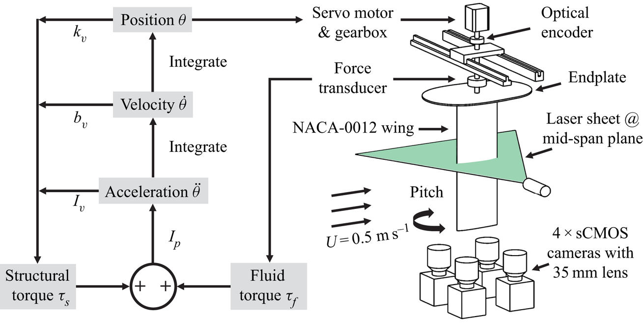
Figure 1 shows the schematic of our experimental set-up. All the experiments are conducted in the Brown University free-surface water tunnel, which has a test section of  $\mathrm {width}~(W) \times \mathrm {depth}~(D) \times \mathrm {length}~(L) = 0.8~\textrm {m}\times 0.6~\textrm {m}\times 4.0~\textrm {m}$. We mount a NACA-0012 wing vertically in the water tunnel, with an endplate on the top to eliminate wingtip vortices at the root. To emulate the behaviour of real-life wings, such as MAV airfoils and energy-harvesting hydrofoils, no endplate is added to the bottom tip of the wing. The wing is made of clear acrylic with a span of
 $s = 0.3~\textrm {m}$ and a chord length of
 $c = 0.1~\textrm {m}$. The pivoting point (i.e. the elastic axis) of the wing is fixed at the midchord,
 $c/2$, throughout all experiments. Detailed wing characteristics can be found in appendixA. To maintain a constant chord-based Reynolds number,
 $Re = \rho U c / \mu = 50\,000$, where
 $\rho$ and
 $\mu$ are water density and dynamic viscosity, respectively, we fix the free-stream velocity at
 $U=0.5~\textrm {m}~\textrm {s}^{-1}$. This velocity is measured by an acoustic Doppler velocimeter (ADV; Nortek Vectrino), positioned at the centre of the
 $W$–
 $D$ plane,
 $2.5~\textrm {m}$ upstream of the wing.
A schematic of the experimental set-up.

2.1. Cyber-physical system implementation
We implement the real-time cyber-physical system (CPS) using MATLAB Simulink with an update rate of 4000 Hz. To introduce the CPS, we start with the governing equation of the system
 \begin{equation} I \ddot{\theta} + b \dot{\theta} + k \theta = \tau_f, \end{equation}
where  $I$,
 $b$ and
 $k$ are the effective inertia, damping and stiffness of the wing, respectively, and
 $\tau _f$ is the fluid torque. The effective inertia,
 $I = I_p+I_v$, is a combination of the physical inertia of the wing,
 $I_p$, and a user assigned virtual inertia,
 $I_v$. Because no physical spring is present in the system and the frictional damping is negligible, we use virtual values to achieve the target stiffness,
 $k = k_v$, and the target damping,
 $b = b_v$. Adding up all the virtual torques, the total virtual structural torque can be calculated as
 \begin{equation} \tau_s = -(k_v \theta + b_v \dot{\theta} + I_v \ddot{\theta}). \end{equation}
Substituting (2.2) into (2.1), we can get
 \begin{equation} I_p \ddot{\theta} = \tau_f + \tau_s. \end{equation}
Now we introduce the real-time control loop depicted in figure 1. The fluid torque exerted on the wing,  $\tau _f$, measured by a six-axis force/torque transducer (ATI 9105-TIF-Delta-IP65), is fed into the loop. After adding the structural torque,
 $\tau _s$ (calculated from the previous time step), the total torque,
 $\tau _f + \tau _s$, is divided by the physical inertia of the wing,
 $I_p$, to get the pitching acceleration,
 $\ddot {\theta }$:
 \begin{equation} \ddot{\theta} = (\tau_f + \tau_s)/I_p. \end{equation}
Next,  $\ddot {\theta }$ is integrated once to get the pitching velocity,
 $\dot {\theta }$, and again to get the pitching position,
 $\theta$. The pitching position signal is used as input to a servomotor (Parker SM233AE), coupled with a gearbox (Automation Direct PGCN23-0525), to pitch the wing. We use an optical encoder (US Digital E3-2500-250-IE-D-D-1), which is independent of the CPS, to record the actual pitching angle. At each time step, the structural torque,
 $\tau _s$, is recalculated using (2.2) based on the new pitching dynamics (
 $\theta$,
 $\dot {\theta }$ and
 $\ddot {\theta }$) and added to
 $\tau _f$ at the next time step to close the control loop. Data from the ADV, the force/torque transducer and the optical encoder are sampled using a data acquisition (DAQ) board (National Instruments PCIe-6353) at a frequency of 4000 Hz. The position signal is also output by the same DAQ board to the servomotor via a motor drive (Advanced Motion Controls DPRALTE-020B080).
Validation of the performance of this real-time cyber-physical system can be found in appendix A. Compared to the velocity loop used by Onoue et al. (Reference Onoue, Song, Strom and Breuer2015), the position loop is less sensitive to noise and more robust because of the double integration. No filtering is required to get a clean and smooth position signal. For plotting purposes only, a zero-phase sixth-order low-pass Butterworth filter is applied to the raw force data so as to smooth out small oscillations. The filter cut-off frequency is set to 25 times the observed pitching frequency. It is important to emphasize that this filter is only employed for post-processing of the data; no filter is used inside the real-time control loop.
2.2. Particle image velocimetry set-up
The flow field around the pitching wing is measured using a time-resolved two-dimensional PIV system shown in figure 1. The laser sheet, created by a double-pulse Nd:YAG laser (200 mJ at 532 nm, Quantel Laser EverGreen 200) with LaVision sheet optics, illuminates the midspan plane of the wing. Because the wing is made of clear acrylic, the laser sheet can pass through the wing, enabling flow field measurement on both sides of the wing. It should be noted that the laser sheet plane is sufficiently far from the wingtip that the tip vortex is excluded from the measurement. The flow is seeded by 50 ${\mathrm {\mu }}$m silver-coated hollow ceramic spheres. Image pairs of the flow field are acquired by four coplanar cameras (LaVision Imager sCMOS,
 $2560\times 2160$ pixels) equipped with 35 mm lenses and mounted beneath the water tunnel. The laser and cameras are synchronized by a Programmable Timing Unit (PTU; LaVision). The PIV images are fed into the LaVision DaVis software (v.10) for image processing. Multi-pass cross-correlation (two passes at
 $64\times 64$ pixels, two passes at
 $32\times 32$ pixels, both with 50 % overlap) is used to calculate velocity vectors from each camera view, and the vector fields of the four cameras are stitched together to form a larger field of view (
 $\sim 4c\times 4c$).
2.3. Non-dimensional parameters
Following Onoue et al. (Reference Onoue, Song, Strom and Breuer2015), we assume the fluid inertia force  $0.5 \rho U^{2} c^{2} s$ to be the dominating scaling force and normalize the stiffness, damping, inertia and fluid torque as
 \begin{equation} k^{*} = \frac{k}{0.5\rho U^{2} c^{2} s},\quad b^{*} = \frac{b}{0.5\rho U c^{3} s},\quad I^{*} = \frac{I}{0.5\rho c^{4} s},\quad \tau_f^{*} = \frac{\tau_f}{0.5\rho U^{2} c^{2} s}. \end{equation}
Therefore, the non-dimensional governing equation of the system becomes
 \begin{equation} I^{*} \ddot{\theta}^{*} + b^{*} \dot{\theta}^{*} + k^{*} \theta^{*} = \tau_f^{*},\end{equation}
where  $\theta ^{*} = \theta$,
 $\dot {\theta }^{*} = \dot {\theta }c/U$ and
 $\ddot {\theta }^{*} = \ddot {\theta }c^{2}/U^{2}$.
It is worth mentioning that the inverse of the non-dimensional stiffness is identical to the commonly used Cauchy number,  $Ca=1/k^{*}$, which describes the ratio between the fluid inertia force and the elastic force (Ishihara et al. Reference Ishihara, Yamashita, Horie, Yoshida and Niho2009; Jin et al. Reference Jin, Kim, Fu and Chamorro2019; Wu et al. Reference Wu, Nowak and Breuer2019). The non-dimensional inertia,
 $I^{*}$, is equivalent to the mass ratio between the wing and ambient fluid (Tzezana & Breuer Reference Tzezana and Breuer2019). The non-dimensional fluid torque,
 $\tau _f^{*}$, is the unsteady moment coefficient of the wing. Another important non-dimensional parameter in the present study, which has appeared in many previous FSI studies (Khalak & Williamson Reference Khalak and Williamson1996; Kim et al. Reference Kim, Cossé, Cerdeira and Gharib2013; Fagley et al. Reference Fagley, Seidel and McLaughlin2016; Menon & Mittal Reference Menon and Mittal2019), is the non-dimensional velocity
 $U^{*}$, defined as
 $U^{*} = U/(2{\rm \pi} f c)$, where
 $f$ is the oscillation frequency. It is important to note that
 $U^{*}$ can have different definitions in the present study, depending on the frequency used to calculate
 $U^{*}$. There are several frequencies of interest in the dynamics of elastically mounted pitching wings, including: (a) the frequency of flow oscillations that may occur even in the absence of structural motions (e.g. the von Kármán vortex shedding frequency described in Menon & Mittal Reference Menon and Mittal2019); (b) the structural (or natural) frequency of the wing,
 $f_s$, calculated based on the spring stiffness and the wing inertia (i.e.
 $f_s = (\sqrt {k/I})/2{\rm \pi}$); and (c) the pitching frequency,
 $f_p$, which arises from the dynamic coupling between the flow and the structure (in the aeroelastic literature, this frequency may be called the flutter or limit-cycle oscillation frequency). In the following sections, we will use
 $U_s^{*}$ to denote
 $U^{*}$ calculated using
 $f_s$ (i.e.
 $U_s^{*} = U/(2{\rm \pi} f_s c)$), and
 $U_p^{*}$ to denote
 $U^{*}$ calculated using
 $f_p$ (i.e.
 $U_p^{*} = U/(2{\rm \pi} f_p c)$).
3. Results and discussion
3.1. Subcritical and supercritical bifurcations
In the present study, we fix the structural damping of the wing at  $b^{*} = 0.13$ and keep the initial AOA at zero. We want to note that different initial AOAs can introduce significant differences in bifurcation behaviours (Dugundji Reference Dugundji2008; Razak, Andrianne & Dimitriadis Reference Razak, Andrianne and Dimitriadis2011; Menon & Mittal Reference Menon and Mittal2019). In the present study, we only focus on the zero initial AOA case. At different wing inertias, we first incrementally increase the Cauchy number,
 $Ca$, by decreasing the wing stiffness,
 $k^{*}$, to define the onset of instability. Then we incrementally decrease
 $Ca$ by increasing
 $k^{*}$ to test for the annihilation of instability and the presence of any hysteresis. The amplitude response of the system,
 $|A|$, is defined using the absolute value of the peak pitching amplitude, and the divergence angle,
 $|\overline {A}|$, is defined as the absolute value of the mean pitching angle. We plot
 $|A|$ and
 $|\overline {A}|$ against the Cauchy number
 $Ca=1/k^{*}$ instead of
 $k^{*}$ because the former can better resemble typical bifurcation diagrams in dynamical systems (Strogatz Reference Strogatz1994).
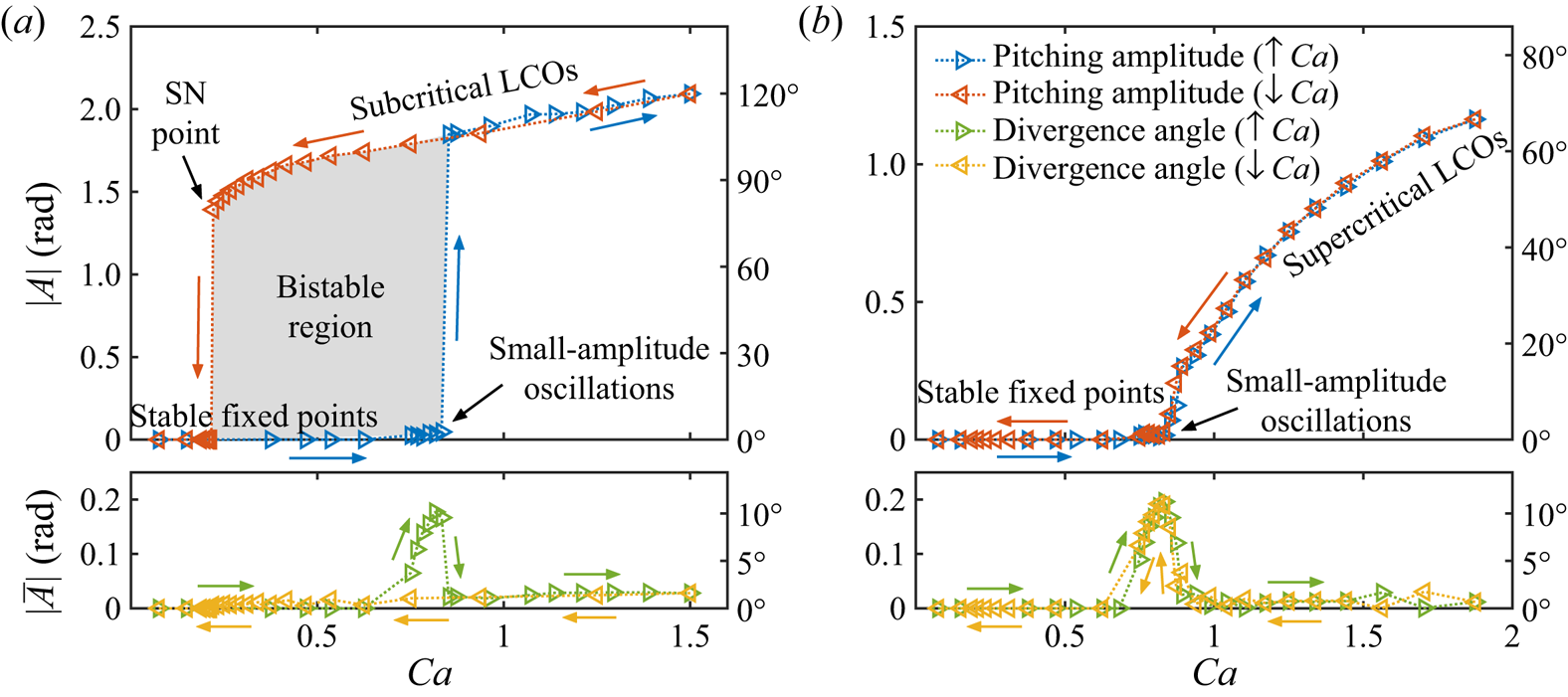
Figure 2 shows the amplitude response of the system at two different wing inertias. When the inertia is relatively high ( $I^{*}=10.6$, figure 2a), as we increase
 $Ca$, the wing first remains stable with a negligible divergence angle. Although the zero divergence angle is always an equilibrium state for an elastically mounted wing with zero initial AOA, this state may not be a stable fixed point in practice. To test for the true stability of the wing, we introduce a small external perturbation, or ‘kick’, into the system. This perturbation is computer-generated by superimposing a short virtual torque to the cyber-physical system. A series of perturbation tests with controlled amplitude variance were conducted to determine a proper perturbation amplitude, so that the system is not pushed into other stability regimes. If zero divergence is a stable fixed point solution, the wing will return to the zero divergence angle after the perturbation. However, if the zero-angle condition is an unstable fixed point, the wing will stay at a non-zero divergence angle at which the fluid torque is balanced by the restoring torque provided by the (virtual) spring. The direction of this angle depends on the direction of the initial perturbation, but both positive and negative angles are possible. This static divergence phenomenon is well characterized in the literature (Dugundji Reference Dugundji2008; Dimitriadis & Li Reference Dimitriadis and Li2009).
Amplitude response of the system at (a)  $I^{*} = 10.60$ and (b)
 $I^{*} = 0.33$, presented in radians on the left
 $y$-axis, and in degrees on the right
 $y$-axis. Note that (a) and (b) share the same legend.

As we continue to increase  $Ca$, the static divergence angle becomes larger and small-amplitude oscillations are observed. In this regime, the pitching amplitude
 $\theta$, velocity
 $\dot {\theta }^{*}$ and acceleration
 $\ddot {\theta }^{*}$ are all small, causing the damping torque
 $b^{*}\dot {\theta }^{*}$ and the inertial torque
 $I^{*}\ddot {\theta }^{*}$ to be negligible. As a result, these deflected small-amplitude oscillations are dominated by the balance between the fluid torque
 $\tau _f^{*}$ and the spring restoring torque
 $k^{*}\theta ^{*}$ around the divergence angle. Although these small-amplitude oscillations are not the main focus of the present study, they should be distinguished from the laminar separation flutter reported in the literature (Poirel, Harris & Benaissa Reference Poirel, Harris and Benaissa2008; Poirel & Yuan Reference Poirel and Yuan2010; Poirel, Metivier & Dumas Reference Poirel, Metivier and Dumas2011; Barnes & Visbal Reference Barnes and Visbal2018), where the oscillations are both driven and limited by the aerodynamic force, and can thus sustain even without the presence a structural spring (Poirel et al. Reference Poirel, Harris and Benaissa2008, figure 8). Moreover, we believe that the small-amplitude oscillations observed in the present study are not strictly stall flutter (Dimitriadis & Li Reference Dimitriadis and Li2009; Bhat & Govardhan Reference Bhat and Govardhan2013), because no obvious hysteresis is observed in the force measurements, and the maximum pitching angle mostly stays below the static stall angle. Rather, we think these small-amplitude oscillations come from the interaction between the random flow disturbance and the structural dynamics (mainly the spring stiffness) of the wing.
As the Cauchy number,  $Ca$, is further increased, we observe a critical value above which the pitching dynamics of the wing transitions from small-amplitude oscillations to large-amplitude LCOs. This transition is reflected by an abrupt jump of the pitching amplitude,
 $|A|$, and a drop of the divergence angle,
 $|\overline {A}|$ (figure 2a). The large-amplitude LCOs are nearly sinusoidal and feature a dominant characteristic frequency. The amplitude of these LCOs continues to increase with
 $Ca$, and the corresponding characteristic frequency decreases with
 $Ca$ (see figure 4a). As we decrease the Cauchy number,
 $Ca$, the large-amplitude LCOs persist even when
 $Ca$ is decreased below the critical value, defining a bistable, hysteretic region, before the pitching amplitude returns to the stable fixed point regime via a saddle-node (SN) point. In this bistable region, the system has two stable solutions (i.e. stable LCOs and stable fixed points) and one unstable solution (i.e. unstable LCOs, not observable in experiments). The divergence angle
 $|\overline {A}|$ remains near zero for the entire decreasing path, creating a small hysteretic region near the critical
 $Ca$. Similar bifurcation behaviours have been reported in the wind tunnel experiments literature (Dugundji Reference Dugundji2008; Dimitriadis & Li Reference Dimitriadis and Li2009; Amandolese et al. Reference Amandolese, Michelin and Choquel2013; Onoue et al. Reference Onoue, Song, Strom and Breuer2015). If we ignore the static divergence angle and relax the constraint in the definition of a Hopf bifurcation that the system has to be a fixed point prior to the bifurcation (Strogatz Reference Strogatz1994), the bifurcation observed in the present experiment possesses every feature of a subcritical Hopf bifurcation, with the critical
 $Ca$ corresponding to the Hopf point. The large-amplitude LCOs observed in this operating condition are hence referred to as subcritical LCOs.
The amplitude response for a wing with a much lower inertia ( $I^{*}=0.33$) is shown in figure 2(b). Again, for small
 $Ca$ values, we perturb the system to test for its true stability. Similar to the high-inertia case, as we increase
 $Ca$, the system experiences static divergence and small-amplitude oscillations around the divergence angle. As
 $Ca$ is further increased, the small-amplitude oscillations become larger and the divergence angle gradually decreases to zero. At even higher values of
 $Ca$, the LCO amplitude continues to increase and the divergence angle remains around zero. As we decrease
 $Ca$, both the pitching amplitude
 $|A|$ and the divergence angle
 $|\overline {A}|$ follow exactly the same path back to the original fixed point regime. No hysteresis or amplitude jump is observed during the experiment. As before, if we ignore the static divergence angle and the initial small-amplitude oscillations, the transition appears to be a supercritical Hopf-type bifurcation. We therefore refer to the large-amplitude LCOs observed in this operating condition as supercritical LCOs. Compared to the subcritical bifurcation, which is often referred to as a hard bifurcation because of the dangerous abrupt amplitude jump and hysteresis, a supercritical bifurcation is usually denoted as a soft bifurcation, which is considered to be safer for many applications (Strogatz Reference Strogatz1994).
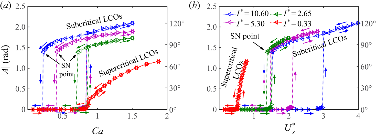
We then test the stability boundaries of the system over a range of wing inertia values. In figure 3(a), the pitching amplitude,  $|A|$, is plotted against the Cauchy number,
 $Ca$. We see that the width of the bistable region shrinks as the inertia decreases, evidenced by the change in the location of the SN point. When the inertia is sufficiently low, the bistable region completely disappears and the subcritical bifurcation becomes supercritical. However, regardless of the bifurcation type (supercritical or subcritical), the onset of instability (i.e. the Hopf point) seems to occur at the same Cauchy number for all wing inertia values. The underlying mechanism of this phenomenon will be discussed in § 3.4.
Pitching amplitude at different wing inertias, plotted against (a) the Cauchy number,  $Ca$, and (b) the
 $f_s$-based non-dimensional velocity,
 $U_s^{*}$. Symbols:
 $\triangleright$, increasing
 $Ca$;
 $\triangleleft$, decreasing
 $Ca$. Note that (a) and (b) share the same legend.

In figure 3(b), we re-plot the pitching amplitude, this time against the  $f_s$-based non-dimensional velocity
 $U_s^{*}$. The connection between
 $Ca$,
 $k^{*}$ and
 $U_s^{*}$ is
 \begin{equation} U_s^{*}=\frac{U}{2{\rm \pi} f_s c}=\sqrt{\frac{I^{*}}{k^{*}}}=\sqrt{Ca\,I^{*}}. \end{equation}
We first observe that, under this scaling, for subcritical bifurcations, the location of the Hopf point rises as the wing inertia increases. After the onset of large-amplitude LCOs, we observe that the pitching amplitude for the three subcritical LCO branches ( $I^{*}=10.60$, 5.30 and 2.65) almost completely overlap, and that these LCOs extinguish at roughly the same critical
 $U_s^{*}$ (i.e. the same SN point), indicating that
 $U_s^{*}$ is a good scaling parameter for this feature of the instability. The critical
 $U_s^{*}$ is actually determined by a critical structural frequency
 $f_s$, because the free-stream velocity
 $U$ and the chord length of the wing
 $c$ remain constant in the present experiment (see (3.1)). Below this critical
 $U_s^{*}$ (above the corresponding critical
 $f_s$), subcritical LCOs cannot sustain. The underlying mechanism for this phenomenon will be discussed in § 3.5. Moreover, the collapse of the subcritical LCO branches indicates that all these LCOs share a universal oscillation mode even though the wing inertia is different. This observation supports Reference Menon and MittalMenon & Mittal's (Reference Menon and Mittal2019) argument that changing the wing inertia only affects the natural frequency of the system. However, we should note that
 $U_s^{*}$ is only able to collapse subcritical LCOs. The behaviour of supercritical LCOs (
 $I^{*}=0.33$) seems to be qualitatively different (i.e. the oscillations are always below the critical
 $U_s^{*}$), suggesting a different mode of oscillation. This is more fully characterized in the next section.
3.2. Structural mode and hydrodynamic mode
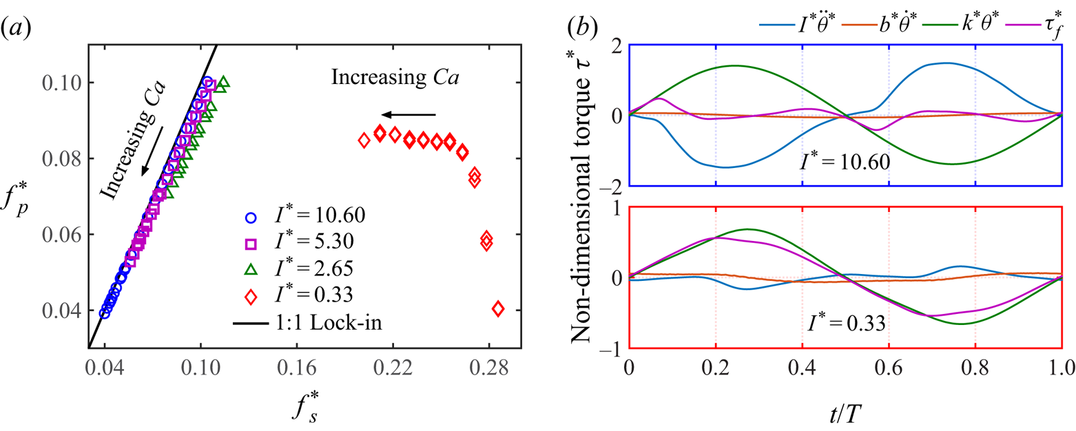
In figure 4(a), we plot the measured pitching frequency of the wing,  $f_p$, against the calculated structural frequency,
 $f_s$, both normalized by the fluid time scale (i.e.
 $f^{*}=fc/U$). Because it is difficult to extract
 $f^{*}_p$ for small-amplitude oscillations (see figure 2), the data shown only correspond to relatively large-amplitude LCOs (i.e. super- and subcritical LCOs, see figure 3). To illustrate how each term in (2.6) affects the pitching dynamics over one cycle, we decompose the non-dimensional torque experienced by the wing into the inertial torque,
 $I^{*}\ddot {\theta }^{*}$, the damping torque,
 $b^{*}\dot {\theta }^{*}$, the spring restoring torque,
 $k^{*}\theta ^{*}$, and the fluid torque,
 $\tau _f^{*}$. The decomposition result is shown in figure 4(b), with the top panel corresponding to the high-inertia case (
 $I^{*}=10.6$) and the bottom panel corresponding to the low-inertia case (
 $I^{*}=0.33$), both at
 $Ca=1.5$.
(a) The frequency response of the wing at four different inertia values. (b)Non-dimensional torques experienced by the wing at  $Ca=1.5$ over one normalized pitching cycle:
 $I^{*}\ddot {\theta }^{*}$, inertial torque;
 $b^{*}\dot {\theta }^{*}$, damping torque;
 $k^{*}\theta ^{*}$, spring restoring torque; and
 $\tau _f^{*}$, fluid torque. Upper panel is for
 $I^{*}=10.60$ and lower for
 $I^{*}=0.33$. Note the
 $y$-scale difference in (b).

We observe that for the high-inertia case ( $I^{*}=10.60$), as
 $Ca$ is varied, the pitching frequency,
 $f^{*}_p$, locks onto the structural frequency,
 $f^{*}_s$ (figure 4a, blue circles). The maximum
 $f^{*}_p$ corresponds to the SN point in the bifurcation diagram (see figure 2a), whereas the minimum
 $f^{*}_p$ corresponds to the highest
 $Ca$. This lock-in phenomenon indicates that the structural force is the dominating force governing the pitching motion, which is supported by the torque decomposition in figure 4(b, top). In this panel, we see that the spring restoring torque,
 $k^{*}\theta ^{*}$, is of similar amplitude, and opposite sign to the inertial torque,
 $I^{*}\ddot {\theta }^{*}$, while the fluid torque,
 $\tau _f^{*}$, and the damping torque,
 $b^{*}\dot {\theta }^{*}$, are relatively small. A similar lock-in phenomenon was observed by Onoue et al. (Reference Onoue, Song, Strom and Breuer2015) and Menon & Mittal (Reference Menon and Mittal2019). In figure 4(a), we also plot the frequency response for the two moderate-inertia cases (
 $I^{*}=5.30$ and
 $2.65$, purple squares and green triangles). The lock-in phenomenon persists in these two cases but
 $f^{*}_p$ is slightly lower than
 $f^{*}_s$, especially for the lower-inertia wing. We attribute this to the increase of effective inertia brought by the added-mass effect, which is more prominent for lower inertia values. The fact that the lock-in phenomenon is observed for all the subcritical LCOs further confirms that these LCOs feature the same oscillation mode, which we denote as the structural mode.
In contrast, for the low-inertia case ( $I^{*}=0.33$), the frequency response (figure 4(a), red diamonds) lies to the right of the
 $1:1$ lock-in line, indicating that the pitching frequency,
 $f^{*}_p$, is always lower than the structural frequency,
 $f^{*}_s$. No lock-in phenomenon is observed. As we increase
 $Ca$, the pitching frequency stays at a relatively constant value (i.e. constant Strouhal number
 $St=f^{*}_p \approx 0.085$), indicating an intrinsic fluid time scale. This suggests that the fluid torque,
 $\tau _f^{*}$, is driving the pitching motion, which is verified by figure 4(b, bottom). It is seen that the spring restoring torque,
 $k^{*}\theta ^{*}$, mainly balances the fluid torque,
 $\tau _f^{*}$. These two torques are in phase because they are of opposite sign in the governing equation (see (2.6)). The fluid torque,
 $\tau _f^{*}$, has a similar magnitude, but a higher frequency, as compared to that of the high-inertia case. However, because of the low
 $I^{*}$, the inertial torque
 $I^{*}\ddot {\theta }^{*}$ stays comparatively small over the entire pitching cycle, causing the frequency of
 $\tau _f^{*}$ to override the structural frequency. The damping torque,
 $b^{*}\dot {\theta }^{*}$, is almost negligible in this case. Therefore, we denote the supercritical LCOs as the hydrodynamic mode.
3.3. Force response and the corresponding flow field
We plot the torque–angle phase diagram,  $\tau _f^{*}$–
 $\theta$, for both the high-inertia case (
 $I^{*}=10.60$) and the low-inertia case (
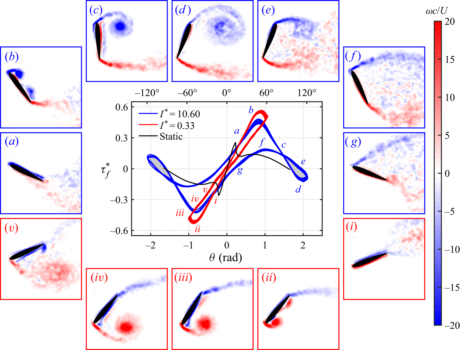
 $I^{*}=0.33$) in the centre of figure 5. The static torque–angle measurement is plotted for comparison. The corresponding phase-averaged flow fields at different time instants are also plotted surrounding that diagram. Because of symmetry, we only show the vorticity fields for half of the pitching cycle. Figure 5(a–g) correspond to the positive half pitching cycle of the high-inertia case (
 $I^{*}=10.60$). Figure 5(i–v) correspond to the negative half pitching cycle of the low-inertia case (
 $I^{*}=0.33$).
Torque–angle phase diagram (centre) for  $I^{*}=10.60$ (structural mode) and
 $I^{*}=0.33$ (hydrodynamic mode) at
 $Ca=1.5$ (the same operating conditions as in figure 4b), and the corresponding vorticity fields (flow direction is left to right): (a–g)
 $I^{*}=10.60$, corresponding to the blue curve; (i–v)
 $I^{*}=0.33$, corresponding to the red curve. See supplementary movies available at https://doi.org/10.1017/jfm.2020.481.

For the high-inertia case, the force response and the corresponding vorticity field are very similar to that observed by Onoue & Breuer (Reference Onoue and Breuer2016). As the wing departs from the zero pitching angle, the fluid torque  $\tau _f^{*}$ starts to grow. The phase diagram shows that
 $\tau _f^{*}$ is non-zero at
 $\theta =0$. This positive intercept is presumably due to the pressure difference between the two sides of the wing, caused by the separated flow on the lower wing surface inherited from the previous cycle (Onoue & Breuer Reference Onoue and Breuer2016). The PIV measurements (figure 5a,b) depict the emergence of a strong LEV, which is attached to the upper surface of the wing, in the fore section. Meanwhile, we observe a patch of vorticity on the aft part of the upper surface, which could be a shear-layer vortex caused by the rolling-up of surface vorticity (Sharma & Visbal Reference Sharma and Visbal2019). The
 $\tau _f^{*}$ value starts to decrease after a peak around
 $\theta \approx 0.82\ (47^{\circ })$ is experienced, corresponding to the shedding of the LEV from the wing surface (figure 5c). Compared to the static measurement, this decrease in
 $\tau _f^{*}$ significantly exceeds the static stall angle,
 $\theta _s$. The maximum value of
 $\tau _f^{*}$ is also amplified approximately by a factor of 2. This transient increase of
 $\tau _f^{*}$ (due to the transient increase of
 $C_L$) and the delay in stall evince the dynamic stall phenomenon (McCroskey Reference McCroskey1982; Eldredge & Jones Reference Eldredge and Jones2019). Although
 $\tau _f^{*}$ is decreasing and the spring restoring torque is increasing, the wing continues to pitch up due to its high inertia, until the maximum pitching amplitude is achieved around
 $\theta \approx 2.09\ (120^{\circ })$.
In Onoue & Breuer (Reference Onoue and Breuer2016, figure 3), the maximum  $\theta$ is around
 $90^{\circ }$. This discrepancy is presumably due to differences in the wing characteristics (i.e. flat plate versus NACA-0012 wing). The
 $\tau _f^{*}$ value goes below zero at roughly the same
 $\theta$ as in the static measurement. At the maximum
 $\theta$, the LEV reaches its maximum size while remaining relatively coherent (figure 5d), before it breaks into smaller-scale structures and fully detaches from the wing surface, evidenced by the disconnection between the leading edge and the LEV feeding shear layer. After arriving at the peak
 $\theta$, the pitching motion starts to reverse. Then
 $\tau _f^{*}$ increases again and experiences another peak, due to the formation, growth and shedding of a secondary LEV caused by the rolling-up of the feeding shear layer (figure 5e,f) (Jantzen et al. Reference Jantzen, Taira, Granlund and Ol2014; Onoue & Breuer Reference Onoue and Breuer2016). The relatively diffusive appearance of the secondary LEV (figure 5e) could be an artifact due to the fact that these vorticity fields are phase-averaged, while the real LEV may exhibit some phase jitter. In the final stage, the restoring torque pulls the wing back to the zero pitching angle, while the flow on the upper wing surface is still separated (figure 5g). This results in the negative intercept of
 $\tau _f^{*}$ at the beginning of the second half of the pitching cycle.
For the low-inertia case, the initial behaviour of the force response and the flow field (figure 5i,ii) is very similar to that of the high-inertia case (figure 5a,b). For both cases,  $\tau _f^{*}$ peaks at a similar angular position
 $\theta \approx 0.82\ (47^{\circ })$, agreeing well with experiments and models by Strickland & Graham (Reference Strickland and Graham1987) and Granlund et al. (Reference Granlund, Ol and Bernal2013), in which the wing undergoes rapid pitching at constant angular velocities. The origin of this peak in
 $\tau _f^{*}$ for both cases is the formation and shedding of the primary LEV. The peak
 $\tau _f^{*}$ is higher for the low-inertia case, presumably due to a stronger LEV defined by a higher reduced frequency and thereby a larger feeding shear-layer velocity (Onoue & Breuer Reference Onoue and Breuer2016, Reference Onoue and Breuer2017).
The primary discrepancy between the high-inertia case and the low-inertia case appears right after the maximum  $\tau _f^{*}$ is achieved. The low-inertia wing does not have enough momentum (due to the low inertia) to keep pitching up when the LEV starts to detach from the wing surface (figure 5iii). Therefore,
 $\theta$ reaches its maximum almost immediately after the peak
 $\tau _f^{*}$ has arrived. As the LEV further sheds from the wing surface, it moves towards the aft part of the wing (figure 5iv) and becomes less coherent (figure 5v). The
 $\tau _f^{*}$ value decreases monotonically and the spring restoring torque gradually brings the wing back to the zero pitching angle. At
 $\theta =0$, the
 $y$-intercept of
 $\tau _f^{*}$ for the low-inertia case is smaller than that of the high-inertia case, because the flow on the suction side of the wing reattaches faster. In the low-inertia case, no secondary peak in
 $\tau _f^{*}$ is observed and the secondary LEV is absent during the pitch reversal. As a result, no negative hysteresis region (figure 5 grey shaded areas) is formed, suggesting that no energy is being transferred from the system to the wake over the pitching cycle (Onoue & Breuer Reference Onoue and Breuer2016). However, this does not necessarily indicate that low wing inertia is more favourable for energy harvesting, as the harvesting efficiency depends on the net area of the hysteretic region.
3.4. Transition to subcritical limit-cycle oscillations
One key feature of the subcritical bifurcation observed for the high-inertia wing is the abrupt jump of the pitching amplitude at the critical  $Ca$ (see figure 2a). In the time domain, when
 $Ca$ is increased above the critical value, the amplitude jump is in fact a gradual transition process, in which the pitching amplitude grows and saturates over a period of around one minute (
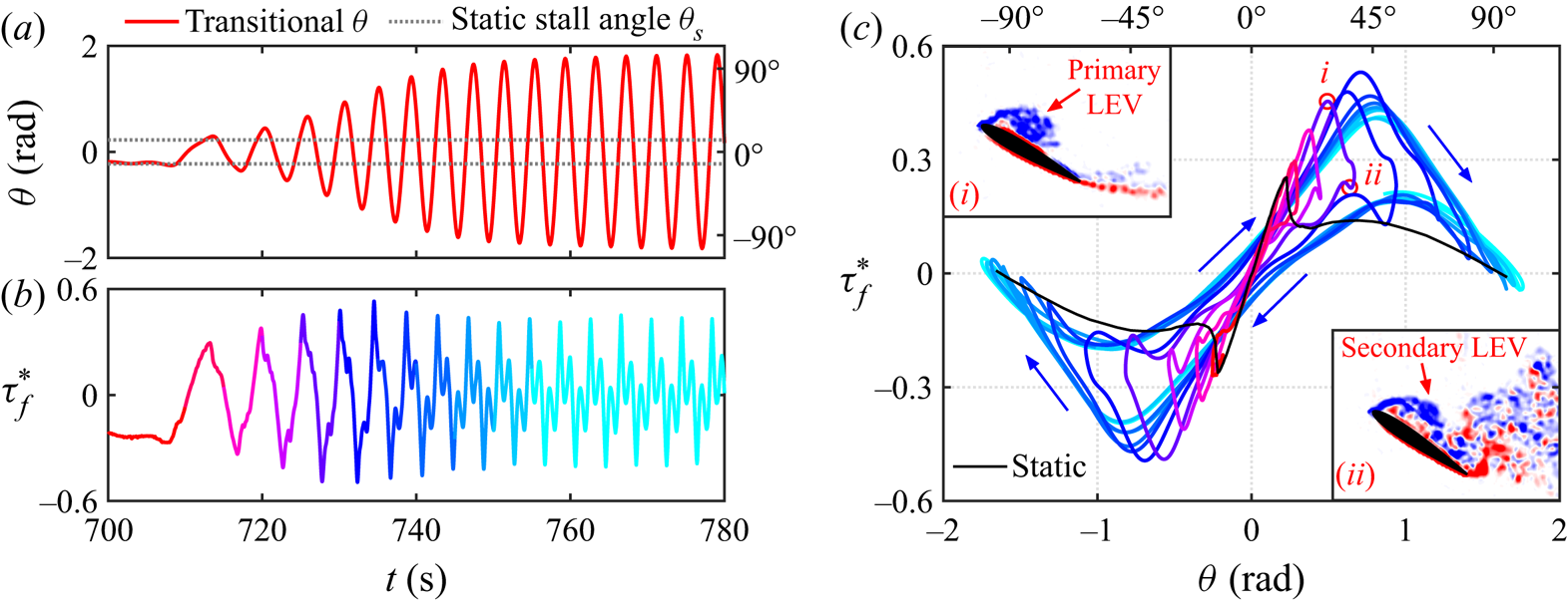
 $\sim$12 cycles). Figure 6(a) shows the time trace of the pitching motion during this transition. Figure 6(b) shows the temporal evolution of the corresponding fluid torque,
 $\tau _f^{*}$. Figure 6(c) shows the transitional
 $\tau _f^{*}$–
 $\theta$ phase diagram. The static measurement is also plotted in black for comparison. In figure 6(b,c), the time dependence of
 $\tau _f^{*}$ is indicated by the colour shade. The red colour represents the starting stage of the transition, whereas the cyan colour indicates the amplitude saturation stage.
Transition to subcritical LCOs in the high-inertia case ( $I^{*}=10.60$) at
 $Ca=0.85$. (a) Time trace of the amplitude transition (red solid line). Grey dotted lines indicate the static stall angle
 $\theta _s$. (b) Temporal evolution of the fluid torque
 $\tau _f^{*}$ during the transition. (c) Transitional torque–angle phase diagram. Insets: Two representative vorticity field showing (i) a primary LEV and (ii) a secondary LEV. The angular positions of these two vorticity fields are indicated by red circles. Insets (i) and (ii) share the same colour bar with figure 5.

Before the transition occurs, the wing undergoes small-amplitude quasi-steady oscillations around its equilibrium divergence angle (see § 3.1). At this stage, the flow on the wing surface is mostly attached (PIV measurements not shown here). As  $Ca$ is increased above the critical value, the spring is not stiff enough to hold the wing below the static stall angle,
 $\theta _s$ (i.e. the grey dotted lines in figure 6a). Once
 $\theta _s$ is exceeded, the flow starts to separate and the wing experiences a sudden drop in
 $\tau _f^{*}$. The spring restoring torque loses its counterpart so that the wing is accelerated to pitch towards the opposite direction. At this very initial stage of the transition, the pitch reversal starts as soon as the separation occurs. However, at the later stage of the transition and when the oscillation saturates, the wing will continue to pitch after the flow separates (i.e. pitching ‘overshoot’), on account of the high inertia. As the wing starts to gain velocity, the flow becomes unsteady and the static stall transitions to dynamic stall. As a result, the stall is delayed and the maximum
 $\tau _f^{*}$ increases because of the formation of LEVs (figure 6c, inset i). This positive feedback loop results in a further increase in the pitching amplitude. Figure 6(c) clearly depicts this transition, showing how the wing departs from the quasi-steady state to the unsteady state. The growth in pitching amplitude is finally limited by the spring restoring torque (see also figure 4b, top), which leads to the amplitude saturation. How this quasi-steady to unsteady transition shapes the stability characteristics of the system will be discussed in § 3.5.
In § 3.3, we have shown that the secondary peak in  $\tau _f^{*}$ during the pitch reversal is associated with the presence of a secondary LEV (figure 5e). Figure 6(c) illustrates how this secondary
 $\tau _f^{*}$ peak emerges and strengthens during the transition, providing evidence for the emergence and development of the corresponding secondary LEV, which is confirmed by vorticity measurements. Figure 6(c, inset ii) shows that a secondary LEV is indeed formed during the pitch reversal, even during the very first few cycles of the transition. Moreover, figure 6(c) also shows that secondary LEVs can exist for a relatively low pitching amplitude (
 $|A| < 1$), which suggests that the absence of the secondary LEV in the low-inertia case (figure 5) is not due to the low pitching amplitude (
 $|A| \approx 1$), but could well be a result of the high pitching frequency, as compared to the high-inertia case. For a high pitching frequency, the feeding shear layer does not have sufficient time to roll up so that the secondary LEV is not able to form in the low-inertia case.
In summary, figure 6 manifests that the onset of the subcritical LCOs depends on the static characteristics (i.e. the static stall angle) of the wing. It also provides a connection between the quasi-steady state and the unsteady state for the pitching dynamics and the fluid torque, which could benefit the modelling of the system. It is important to note that, although the main focus of this section is to reveal the underlying dynamics and flow physics of a subcritical transition, the mechanism that triggers this transition (i.e. the pitching amplitude exceeding the static stall angle) also applies to a supercritical transition. However, while the subcritical transition has a prolonged amplitude evolution (figure 6a), the supercritical transition is almost instantaneous, due to the low wing inertia. This explains why the onset of LCOs scales well with  $Ca$ (figure 3a) in spite of the different bifurcation types. The reason why the system can settle into different LCO solutions will be discussed next in § 3.5.
3.5. System stability from the perspective of energy transfer
Now we characterize the stability of our system from the perspective of energy transfer between the fluid and the supporting structure. Morse & Williamson (Reference Morse and Williamson2009) were among the first to introduce the energy approach for predicting VIVs of an elastically mounted translating cylinder. In the context of passively pitching wings, this approach has been shown to be effective for predicting the stability of small-amplitude ( $|A|<6^{\circ }$, Bhat & Govardhan Reference Bhat and Govardhan2013) and moderate-amplitude (
 $|A|<50^{\circ }$, Menon & Mittal Reference Menon and Mittal2019) flow-induced oscillations. Here we extend this approach to the large-amplitude (
 $50^{\circ }<|A|<120^{\circ }$) regime.
As noted before (Onoue et al. Reference Onoue, Song, Strom and Breuer2015; Menon & Mittal Reference Menon and Mittal2019), the flow-induced pitching motion is well described by a sinusoidal motion. This is also true in the current measurements ( $R^{2} > 0.98$). Thus, if we assume that the pitching motion can be described by
 \begin{equation} \theta = |A| \sin (2{\rm \pi} f_p t), \end{equation}
where  $|A|$ is the pitching amplitude and
 $f_p$ is the pitching frequency, we can prescribe the amplitude and frequency of the motion, measure the fluid torque,
 $\tau _f$, and integrate the equation of motion (2.6) over
 $n$ cycles to obtain the cycle-averaged energy transfer between the fluid and the structure:
 \begin{equation} E = \frac{1}{n} \int_{t_0}^{t_0+nT} (\tau_f \dot{\theta} - b \dot{\theta}^{2})\, \textrm{d} t. \end{equation}
For the results presented here, we have used  $n = 20$ and swept
 $f_p$ from 0.15 to 0.6 Hz with a step size of 0.05 and
 $|A|$ from 0 to 2.5 rad with a step size of 0.175. The
 $\tau _f\dot {\theta }$ term represents the power extracted by the wing from the ambient fluid, and the
 $b\dot {\theta }^{2}$ term represents the power dissipated by the structural damping (Menon & Mittal Reference Menon and Mittal2019). Following Onoue etal. (Reference Onoue, Song, Strom and Breuer2015), we multiply
 $E$ by the pitching frequency,
 $f_p$, and normalize the equation to get the power coefficient of the system:
 \begin{equation} C_p = \frac{f_p^{*}}{n} \int_{t_0}^{t_0+nT} (\tau_f^{*} \dot{\theta}^{*} - b^{*} \dot{\theta}^{*2})\, \textrm{d} t^{*}. \end{equation}
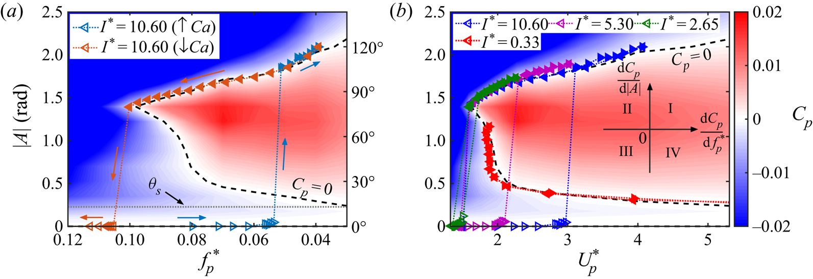
The power coefficient map is shown in figure 7, with the  $x$-axis represented by
 $f_p^{*}$ in figure 7(a) and by
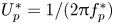 $U_p^{*}=1/(2{\rm \pi} f_p^{*})$ in figure 7(b). In both plots, red, white and blue represent regions of power extraction (
 $C_p>0$), balance (
 $C_p=0$) and dissipation (
 $C_p<0$), respectively. The power balance (
 $C_p=0$) curve is indicated by black dashed lines. The value
 $|A|=0$ is also a possible solution for power balance. We wish to note that, although figure 7 reflects the power coefficient map of one particular damping value (
 $b^{*}=0.13$), the power coefficient map of other damping values can be easily generated by simply varying
 $b^{*}$ in (3.4). This demonstrates the universality of the energy approach for analysing systems with different structural damping values (Morse & Williamson Reference Morse and Williamson2009; Menon & Mittal Reference Menon and Mittal2019). To connect the power coefficient map with the previously discussed system stability boundaries, we re-plot the amplitude response data, from figures 2(a) and 3(b), onto figures 7(a) and 7(b), respectively. To make the connection between figures 7(a) and 2(a) more intuitive, we plot the
 $x$-axis of figure 7(a) using a reverse scale, so that the shape of the bifurcation diagram remains relatively consistent in these two plots. In both figures7(a) and 7(b), the frequency for large-amplitude LCOs (i.e. solid markers) is the measured pitching frequency
 $f_p^{*}$. For the data points with zero- or small-amplitude oscillations (i.e. hollow markers), the frequency is the structural frequency
 $f_s^{*}$ (see § 3.2).
(a) Contour plot of the power coefficient,  $C_p$, overlaid by the amplitude response of the system at
 $I^{*}=10.6$. The zero power coefficient contour is indicated by black dashed lines. The static stall angle
 $\theta _s$ is labelled by a grey dotted line. Note the reverse scale of the
 $x$-axis. (b) Power coefficient map plotted against the non-dimensional velocity, overlaid by the amplitude response of the system at different inertia values. Inset: A diagram illustrating the four quadrants of the power coefficient gradient:
 $x$-axis,
 $\mathrm {d} C_p/\mathrm {d}\,f_p^{*}$;
 $y$-axis,
 $\mathrm {d} C_p/\mathrm {d} |A|$.

Comparing figure 7(a) with the energy map of Menon & Mittal (Reference Menon and Mittal2019, figure 13), we see that, although the frequency range of these two maps is quite different (i.e.  $0.03 \leq f_p^{*} \leq 0.12$ versus
 $0.10<f_p^{*}<0.75$), the general shape looks similar for the overlapped amplitude range (i.e.
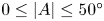 $0 \leq |A| \leq 50^{\circ }$). Both maps show that the wing extracts more energy from the ambient fluid when the pitching frequency is low, and dissipates more energy when the pitching frequency is high (note the reverse
 $x$-axis in figure 7a). However, the detailed shapes of the power balance curve (
 $C_p=0$) are very different in these two maps. The
 $C_p=0$ curve seems to extend to
 $(\,f_p^{*},|A|)=(0,0)$ in figure 7(a), but stays relatively vertical and has a non-zero
 $x$-intercept in figure 13 of Menon & Mittal (Reference Menon and Mittal2019). Moreover,
 $|A|=0$ is part of the
 $C_p=0$ curve in figure 7(a), but not in figure 13 of Menon & Mittal (Reference Menon and Mittal2019). We believe that these differences mainly come from the different initial AOAs used in these two studies (i.e.
 $0^{\circ }$ versus
 $15^{\circ }$). It has been shown by Dugundji (Reference Dugundji2008), Razak etal. (Reference Razak, Andrianne and Dimitriadis2011) and Menon & Mittal (Reference Menon and Mittal2019, figure 3) that different initial AOAs can lead to significantly different stability characteristics, which suggests that the power coefficient map (or the energy map) of a zero-initial-AOA wing and a
 $15^{\circ }$-initial-AOA wing can be quite different.
Comparing the power coefficient map and the amplitude response reveals many interesting features. Figure 7(a) shows that, for  $I^{*}=10.60$, large-amplitude LCOs fall exactly on the upper branch of the
 $C_p=0$ curve. This is expected because the self-sustained flow-induced oscillations represent a condition of energy balance (Morse & Williamson Reference Morse and Williamson2009; Menon & Mittal Reference Menon and Mittal2019). We have shown in § 3.2 that the subcritical LCOs for
 $I^{*}=10.60$ represent a structural mode, where the pitching frequency locks onto the structural frequency. This means that, for any data point representing subcritical LCOs, its
 $x$-coordinate (i.e.
 $f_p^{*}$) is constrained by
 $k^{*}$ and
 $I^{*}$, so that it is only free to move in the
 $y$-direction (i.e. change
 $|A|$) under external perturbations. If
 $|A|$ increases (or decreases), the system will enter the blue region where
 $C_p<0$ (or the red region where
 $C_p>0$) and go back to the equilibrium solution (
 $C_p=0$) because of power dissipation (or power extraction). Based on this analysis, we can deduce the stability criterion for the structural mode (Menon & Mittal Reference Menon and Mittal2019):
 \begin{equation} C_p=0 \quad\text{and}\quad \frac{\mathrm{d} C_p}{\mathrm{d} |A|} < 0. \end{equation}
The upper branch of the  $C_p=0$ curve satisfies this criterion, so that it is a stable equilibrium solution for subcritical LCOs. The x-axis (i.e.
 $|A|=0$) also represents a stable equilibrium for the same reason. In contrast, the lower branch of the
 $C_p=0$ curve represents an unstable equilibrium solution, because its power gradient along the
 $y$-direction is positive (i.e.
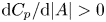 $\mathrm {d} C_p/\mathrm {d} |A| > 0$). The existence of multiple (stable LCO, unstable LCO and stable fixed point) solutions is an important feature of a subcritical Hopf bifurcation, which has been discussed in § 3.1. Revealing the unstable equilibrium solution, which is not possible in passive experiments, is one of the benefits for adopting the energy approach.
Figure 7(b) provides insights into the system stability for other wing inertia values. Because the measured pitching frequency,  $f_p$ (instead of
 $f_s$), is used to calculate
 $U_p^{*}$ for the large-amplitude LCOs, we see that the amplitude response of the subcritical LCOs (
 $I^{*}=10.60$, 5.30 and 2.65) collapse remarkably well, as compared to figure 3(b). All these subcritical LCOs, regardless of their inertia values, fall onto the upper
 $C_p=0$ branch, for the reason discussed above. Moreover, the power coefficient map explains why there exists a critical
 $U_p^{*}$, below which the subcritical LCOs cannot sustain. This is because, below this critical
 $U_p^{*}$ (or above the corresponding critical
 $f_p^{*}$), the power coefficient of the system is negative (
 $C_p<0$). More power is damped by the structural damping than extracted from the fluid, so that the power of the system is insufficient to sustain large-amplitude LCOs. The underlying flow physics causing the decrease of
 $C_p$ requires further investigations.
For  $I^{*}=0.33$, we see that supercritical LCOs fall onto the lower branch of the
 $C_p=0$ curve. As discussed earlier, this lower branch is an unstable equilibrium solution for the structural mode. However, its stability has a different nature for the hydrodynamic mode. In the structural mode, the pitching frequency is constrained by the structural frequency, so that the stability of an equilibrium solution is determined by
 $\mathrm {d} C_p/\mathrm {d} |A|$ (see (3.5)). In contrast, for the hydrodynamic mode, because the oscillation is dictated by the fluid force (see figure 4b, bottom), the system is not constrained to move vertically in the energy map, but is free to move in both the
 $|A|$-direction and the
 $f_p^{*}$-direction. On the lower branch of the
 $C_p=0$ curve, if the system is perturbed to enter the blue region where
 $C_p<0$ (or the red region where
 $C_p>0$),
 $f_p^{*}$ can in turn decrease (or increase) to accommodate power dissipations (or power extractions), and the system will thus return to the equilibrium solution (
 $C_p=0$) again. Therefore, the lower branch of the
 $C_p=0$ curve (
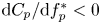 $\mathrm {d} C_p/\mathrm {d} f_p^{*} < 0$) is a stable equilibrium solution for supercritical LCOs.
It is important to note that, because the system is free to move vertically as well, 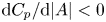 $\mathrm {d} C_p/\mathrm {d} |A| < 0$ can also contribute to the stability of supercritical LCOs. Therefore, the stability criterion for the hydrodynamic mode is
 \begin{equation} C_p=0 \quad\text{and}\quad \left(\frac{\mathrm{d} C_p}{\mathrm{d} |A|} < 0 \quad\hbox{or}\quad \frac{\mathrm{d} C_p}{\mathrm{d} f_p^{*}} < 0 \right). \end{equation}
Following this criterion, the upper branch of the  $C_p=0$ curve and
 $|A|=0$ are also stable equilibrium solutions for the hydrodynamic mode. However, this does not mean that the low-inertia system can have multiple equilibrium solutions at a given
 $Ca$, because
 $Ca$ does not have a one-to-one correspondence with
 $f_p^{*}$ in the hydrodynamic mode. The specific combination of
 $|A|$ and
 $f_p^{*}$ depends on how much power is extracted from the fluid. The selection of different stable equilibrium solutions further confirms the intrinsic difference between the hydrodynamic mode and the structural mode.
Now we can summarize and visualize the stability criterion for the structural mode and the hydrodynamic mode. As shown by (3.5) and (3.6), the common prerequisite for stability for these two oscillation modes is  $C_p=0$. To examine the stability of the
 $C_p=0$ curve, we visualize the sign of
 $\mathrm {d} C_p/\mathrm {d} f_p^{*}$ and
 $\mathrm {d} C_p/\mathrm {d} |A|$ using a quadrant diagram, as shown by the inset of figure 7(b). For the structural mode, the system is stable in quadrants III and IV (including the negative
 $y$-axis), and unstable in quadrants I and II (including the
 $x$-axis and the positive
 $y$-axis). For the hydrodynamic mode, the system is stable in quadrants II, III and IV (including the negative
 $x$- and
 $y$-axis), and unstable only in quadrant I (including the positive
 $x$- and
 $y$-axis). As discussed earlier, for the present system, the
 $C_p=0$ curve has three branches. The upper branch is in quadrant III, so it is a stable solution for both oscillations modes. The lower branch is in quadrant II, so it is a stable solution for the hydrodynamic mode and an unstable solution for the structural mode. The
 $|A|=0$ branch lies on the negative
 $y$-axis, so it is a stable solution for both oscillation modes again.
One critical question in the present study is why the bifurcation is subcritical for the structural mode and supercritical for the hydrodynamic mode. The power coefficient map provides us with some insights. As shown in figure 7(b), for all wing inertias, near the transitional  $U_p^{*}$ values, the stability of the system, indicated by the power coefficient map, is a stable equilibrium at
 $|A|=0$. In theory, without any external perturbations, the system should stay at this stable fixed point solution for any
 $U_p^{*}$. However, we should note that the power coefficient map only identifies the stability of (near-) sinusoidal symmetric oscillations. The stability of the static divergence and quasi-steady small-amplitude oscillations is not accessible from this map. In our experiments, as
 $Ca$ is increased, the wing first bifurcates into a static divergence angle, which brings asymmetry to the problem. Then the system develops small-amplitude oscillations around this divergence angle (§ 3.1). As shown in figure 6(a), after the pitching amplitude exceeds the static stall angle,
 $\theta _s$, unsteady oscillations start near
 $(f_p^{*},|A|)=(0,\theta _s)$, which presumably falls into the power extraction regime (i.e. the red region, see figure 7a). In this regime, the system has two possible evolution paths depending on the oscillation mode.
(i) For the structural mode, because of the constraint in the pitching frequency discussed above,
 $f_p^{*}$ has to gradually develop into $f_s^{*}$. In this process, the system keeps gaining energy from the ambient fluid ($C_p>0$) and finally settles to the upper $C_p=0$ branch (3.5), which results in the abrupt jump in pitching amplitude, defining a subcritical-type bifurcation. The width of the bistable region is determined by the difference between the onset $f^{*}$, which varies with $I^{*}$ because the onset $k^{*}$ is fixed (§ 3.4), and the critical (saddle-node) $f^{*}$, which is unchanged for any combination of $I^{*}$ and $k^{*}$. This explains the shrinking of the bistable region for different wing inertias (figure 3).
(ii) For the hydrodynamic mode, however, without the constraint in
$f_p^{*}$, the system can pick up the lowest possible $|A|$ on the lower $C_p=0$ curve as a stable solution after the transition from quasi-steady oscillations (3.6). This results in a smooth connection between the deflected small-amplitude oscillations and the symmetric large-amplitude LCOs, which creates a supercritical-type bifurcation.


For both paths, the quasi-steady to unsteady transition described in § 3.4 acts as a triggering mechanism for the onset of large-amplitude LCOs. Unveiling this triggering mechanism is of help towards creating a proper low-order model for the system.
4. Conclusion
We have performed water tunnel experiments to examine the stability boundaries of a rigid but flexibly mounted NACA-0012 wing at a Reynolds number of 50 000. We fixed the structural damping of the wing at a small value and systematically varied the torsional stiffness to explore the stability boundaries for different wing inertias. A subcritical bifurcation which features an abrupt amplitude jump and hysteretic bistability was observed for high-inertia wings, whereas a supercritical bifurcation in which the amplitude response varies smoothly with the control parameter without hysteresis was observed for a low-inertia wing. For both types of bifurcations, we showed that the onset of large-amplitude flow-induced oscillations scales with the Cauchy number,  $Ca$. For high-inertia wings, the amplitude and the saddle-node point of subcritical LCOs were reported to scale with the non-dimensional velocity,
 $U^{*}$. Frequency response and force decomposition suggested that subcritical LCOs were dominated by the inertial force, corresponding to a structural mode, while supercritical LCOs were regulated by the fluid force, corresponding to a hydrodynamic mode. The force response was associated with the flow dynamics to explain the difference between the structural mode and the hydrodynamic mode. Two unique phenomena related to the structural mode, namely the frequency lock-in and the presence of a secondary LEV, were reported. We examined the transition to subcritical LCOs in detail, and it was shown that this transition depends on the static characteristics of the wing, and the emergence of the secondary LEV was an important feature of the transition. Finally, we adopted an energy approach to characterize the stability of the system. The stable equilibrium solution for the hydrodynamic mode was shown to be unstable for the structural mode because of the frequency lock-in phenomenon, which further resulted in the distinctive super- and subcritical bifurcations for these two modes.
Acknowledgments
This work is funded by the Air Force Office of Scientific Research, Grant FA9550-18-1-0322, managed by Dr G. Abate. The authors thank D. Harris and members of the Breuer Lab at Brown University, as well as J. Seidel, C. Fagley and A. Jirasek at the US Air Force Academy, for many helpful discussions and insights.
Declaration of interests
The authors report no conflict of interest.
Supplementary movies
Supplementary movies are available at https://doi.org/10.1017/jfm.2020.481.
Appendix A. System characterization
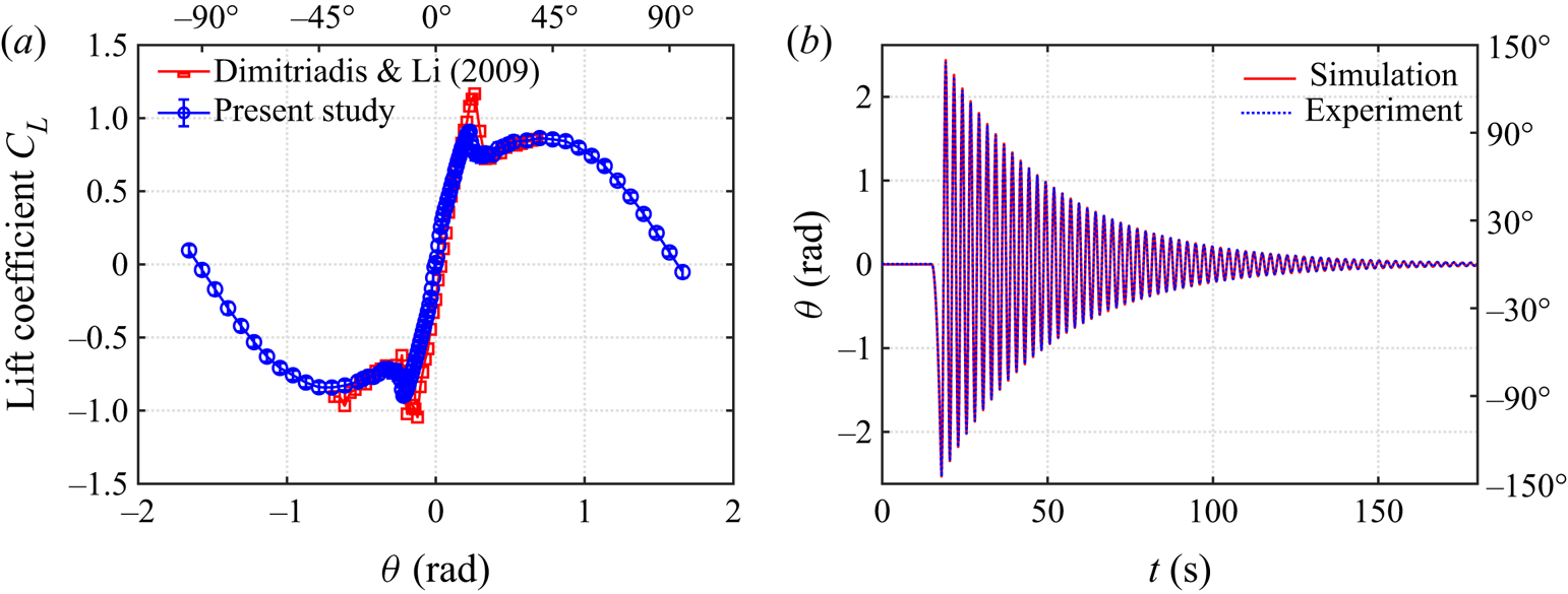
We characterize our NACA-0012 wing by measuring the static lift force  $L$ at different pitching angles. The lift coefficient,
 $C_L$, defined as
 $C_L=L/(0.5 \rho U^{2} c s)$, is plotted against the pitching angle
 $\theta$ in figure 8(a). The measured lift coefficients matches well with previous wind tunnel experiments by Dimitriadis & Li (Reference Dimitriadis and Li2009).
(a) Characterization of the wing. (b) Validation of the cyber-physical system.

We validate our cyber-physical system by conducting free oscillation (‘ring-down’) experiments. The ring-down experiments are conducted in air to exclude the nonlinear fluid damping effect. We apply a short-time constant-torque impulse to the wing using the cyber-physical system, after which we record and analyse the decay of the free damped oscillations. Figure 8(b) shows that the measured pitching decay agrees very well with the simulated decay, which is derived based on the virtual inertia, stiffness and damping, indicating that our cyber-physical system can accurately simulate physical structural dynamics of the system.
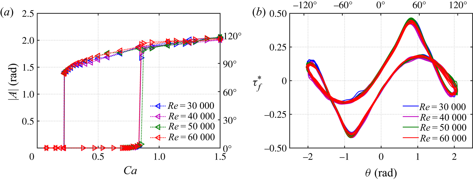
Appendix B. Effect of the Reynolds number
One issue of interest is whether the scaling used in explaining the flow-induced instability boundaries are appropriate(§ 3.1), and to what extent the phenomena are affected by the Reynolds number. These effects are tested by repeating the bifurcation tests for the high-inertia case ( $I^{*}=10.6$) at four different flow speeds
 $U=0.3\text {--}0.6~\textrm {m}~\textrm {s}^{-1}$. The resulting Reynolds number varies from
 $Re=30\,000$ to
 $60\,000$. The virtual structural parameters (
 $I_v$,
 $b_v$ and
 $k_v$) are varied to match the non-dimensional parameters (
 $I^{*}$,
 $b^{*}$ and
 $k^{*}$). The results are shown in figure 9. Figure 9(a) shows that, as the Reynolds number is varied, the amplitude response remains almost the same, despite some subtle changes in the pitching amplitude and the critical
 $Ca$. Taking
 $Ca=1.5$ and plotting the corresponding non-dimensional torque–angle phase diagram in figure 9(b), we observe that the phase diagrams of the four different Reynolds numbers collapse very well. These results indicate that the Reynolds number has a very minor effect on the present experimental results, which agrees with Onoue et al. (Reference Onoue, Song, Strom and Breuer2015). The robustness of our non-dimensionalization is also justified by the unchanging amplitude response and phase diagram. However, we should note that the effect of Reynolds number also depends on the choice of the structural damping
 $b^{*}$. In the present experiments, the structural damping is fixed at a very small value
 $b^{*}=0.13$. At a higher
 $b^{*}$, the Reynolds number can have a prominent effect on the flow-induced oscillations (see figure 12 in Onoue et al. Reference Onoue, Song, Strom and Breuer2015).
(a) Amplitude response of the high-inertia case ( $I^{*}=10.60$) at four different Reynolds numbers and (b) the corresponding torque–angle phase diagram at
 $Ca=1.5$.