1 Introduction
The study of waves in magnetohydrodynamic approximation (MHD) applicable to highly collisional magnetised plasmas has a long history (Danov & Ruderman Reference Danov and Ruderman1983; Roberts Reference Roberts1985). There have been many interfacial flows of interest over the years in MHD which have taken up much of the literature on the subject with applications to astrophysics (Edwin & Roberts Reference Edwin and Roberts1986), geophysics (Barcilon & Fitzjerald Reference Barcilon and Fitzjerald1985) and to magnetic industrial liquids (Gerbeau, Bris & Lelièvre Reference Gerbeau, Bris and Lelièvre2006). Unlike the plasma considered in this paper, Roberts considered waves in a compressible plasma. The types of waves which we are interested in this paper are surface waves in three dimensions along a contact discontinuity. The study of surface waves in hydrodynamics began with the seminal paper by Korteweg & de Vries (Reference Korteweg and de Vries1895) where they employed the approximations of long wavelength and small amplitude. Since this ground-breaking paper, a further fundamental study by Benjamin (Reference Benjamin1967) where a stratified fluid was considered leading to the celebrated Benjamin–Ono (BO) equation. The equation governing the wave propagation includes the Hilbert transform of the second derivative. Since then, there have been many instances where these two fundamentally important equations, i.e. KdV or BO, have appeared.
Benjamin further extended his analysis by expanding the dispersion equation and including weak nonlinearity, later extended for three dimensions by Kim & Akylas (Reference Kim and Akylas2006). A new direction of development is the implementation of external fields (e.g. electric or magnetic). There has been an extensive amount of work in fluid systems with external fields (electric and magnetic) both in two and three dimensions, see e.g. Hunt (Reference Hunt2013) for studies with electric fields, and Roberts (Reference Roberts1985) with magnetised plasmas which deal in the case of compressible fluids.
Set-up.

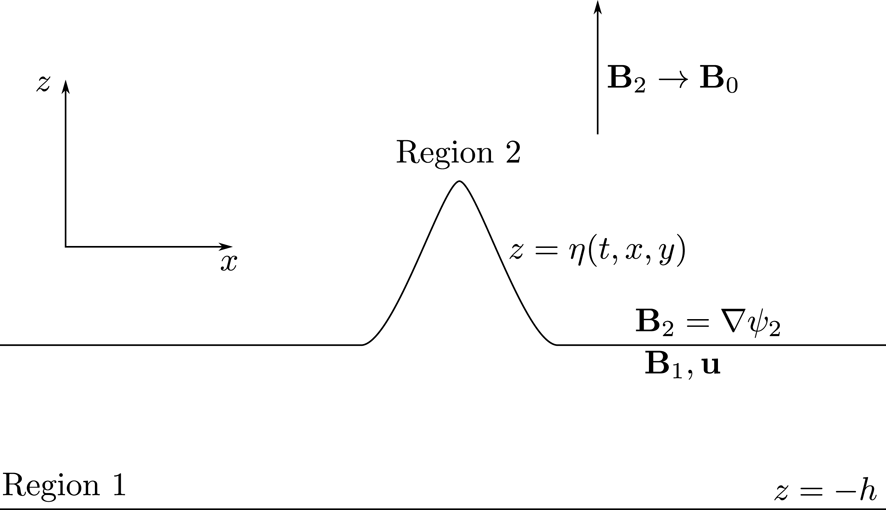
As an introduction, let us recall briefly the paper of Danov & Ruderman (Reference Danov and Ruderman1983). This work is essentially an extension of the original paper on the subject introduced by Korteweg & de Vries (Reference Korteweg and de Vries1895) in fluids to include a magnetic field. A schematic view of their problem set-up is given in figure 1. The fluid (in region 1) defined by
 $-h\leqslant z\leqslant \unicode[STIX]{x1D702}(t,x)$
is perfectly conducting and the region above the fluid (region 2) is perfectly insulating. We assume that fluid 2’s density is small so it does not contribute to the dynamics. The magnetic field in region 2 is current free and as
 $z\rightarrow \infty$
, the magnetic field tends to a constant. In region
 $2$
, there is no flow and the magnetic field satisfies the following conditions:
 $$\begin{eqnarray}\unicode[STIX]{x1D735}\boldsymbol{\cdot }\boldsymbol{B}_{2}=0,\quad \unicode[STIX]{x1D735}\times \boldsymbol{B}_{2}=\mathbf{0},\end{eqnarray}$$
which means that there is a scalar potential,
 $\boldsymbol{B}_{2}=\unicode[STIX]{x1D735}\unicode[STIX]{x1D713}_{2}$
which satisfies the Laplace equation,
 $$\begin{eqnarray}\frac{\unicode[STIX]{x2202}^{2}\unicode[STIX]{x1D713}_{2}}{\unicode[STIX]{x2202}x^{2}}+\frac{\unicode[STIX]{x2202}^{2}\unicode[STIX]{x1D713}_{2}}{\unicode[STIX]{x2202}z^{2}}=0.\end{eqnarray}$$
In region
 $1$
, the usual equations of MHD hold,
 $$\begin{eqnarray}\displaystyle & \displaystyle \frac{\text{D}\boldsymbol{u}}{\text{D}t}=-\frac{1}{\unicode[STIX]{x1D70C}}\unicode[STIX]{x1D735}\left(p+\frac{|\boldsymbol{B}_{1}|^{2}}{2\unicode[STIX]{x1D707}_{0}}\right)-g\boldsymbol{e}_{z}+\frac{1}{\unicode[STIX]{x1D70C}\unicode[STIX]{x1D707}_{0}}(\boldsymbol{B}_{1}\boldsymbol{\cdot }\unicode[STIX]{x1D735})\boldsymbol{B}_{1}, & \displaystyle\end{eqnarray}$$
 $$\begin{eqnarray}\displaystyle & \displaystyle \frac{\text{D}\boldsymbol{B}_{1}}{\text{D}t}=(\boldsymbol{B}_{1}\boldsymbol{\cdot }\unicode[STIX]{x1D735})\boldsymbol{u}. & \displaystyle\end{eqnarray}$$
In region 1, it is convenient to use streamfunctions from which the velocity and magnetic field can be derived
 $$\begin{eqnarray}\boldsymbol{u}=-\frac{\unicode[STIX]{x2202}\unicode[STIX]{x1D711}}{\unicode[STIX]{x2202}z}\boldsymbol{e}_{x}+\frac{\unicode[STIX]{x2202}\unicode[STIX]{x1D711}}{\unicode[STIX]{x2202}x}\boldsymbol{e}_{z},\quad \boldsymbol{B}=-\frac{\unicode[STIX]{x2202}\unicode[STIX]{x1D713}}{\unicode[STIX]{x2202}z}\boldsymbol{e}_{x}+\frac{\unicode[STIX]{x2202}\unicode[STIX]{x1D713}}{\unicode[STIX]{x2202}x}\boldsymbol{e}_{z}.\end{eqnarray}$$
Use of streamfunctions reduces the problems of finding the velocity and magnetic field components to just two scalar functions. The interface between the plasma and magnetic field is a tangential discontinuity. On
 $z=\unicode[STIX]{x1D702}(t,x)$
 $$\begin{eqnarray}\boldsymbol{B}\boldsymbol{\cdot }\hat{\boldsymbol{n}}=0,\quad \hat{\boldsymbol{n}}=\frac{-\unicode[STIX]{x2202}_{x}\unicode[STIX]{x1D702}\boldsymbol{e}_{x}+\boldsymbol{e}_{z}}{\sqrt{1+(\unicode[STIX]{x2202}_{x}\unicode[STIX]{x1D702})}^{2}},\end{eqnarray}$$
the continuity of total pressure across the interface
 $$\begin{eqnarray}\left[p+\frac{|\boldsymbol{B}|^{2}}{2\unicode[STIX]{x1D707}_{0}}\right]_{1}^{2}=0,\end{eqnarray}$$
and finally the free surface equation
 $$\begin{eqnarray}\frac{\unicode[STIX]{x2202}\unicode[STIX]{x1D702}}{\unicode[STIX]{x2202}t}+u\frac{\unicode[STIX]{x2202}\unicode[STIX]{x1D702}}{\unicode[STIX]{x2202}x}=w.\end{eqnarray}$$
At the lower boundary,
 $z=-h$
, we can state
 $$\begin{eqnarray}w=0,\quad B_{z}=0.\end{eqnarray}$$
The weakly nonlinear analysis is carried out and the magnetic fields are perturbed from the base state,
 $\boldsymbol{B}_{0}$
. The coordinates are then transformed as
 $$\begin{eqnarray}X=\unicode[STIX]{x1D700}(x-c_{0}t),\quad T=\unicode[STIX]{x1D700}^{2}t,\end{eqnarray}$$
where
 $c_{0}$
is the gravity wave speed
 $c_{0}=\sqrt{gh}$
. Giving the equation for the free surface as
 $$\begin{eqnarray}\frac{\unicode[STIX]{x2202}\unicode[STIX]{x1D702}_{1}}{\unicode[STIX]{x2202}T}+b\unicode[STIX]{x1D702}_{1}\frac{\unicode[STIX]{x2202}\unicode[STIX]{x1D702}_{1}}{\unicode[STIX]{x2202}X}+\unicode[STIX]{x1D6FD}\mathscr{H}\left(\frac{\unicode[STIX]{x2202}^{2}\unicode[STIX]{x1D702}_{1}}{\unicode[STIX]{x2202}X^{2}}\right)=0,\end{eqnarray}$$
where
 $$\begin{eqnarray}b=\frac{3gh+v_{A}^{2}\cos ^{2}\unicode[STIX]{x1D6FC}}{2c_{0}h},\quad \unicode[STIX]{x1D6FD}=\frac{v_{A}^{2}h\cos \unicode[STIX]{x1D6FC}}{2c_{0}},\end{eqnarray}$$
where
 $v_{A}=B_{0}/\sqrt{\unicode[STIX]{x1D707}_{0}\unicode[STIX]{x1D70C}_{0}}$
. The operator
 $\mathscr{H}(\boldsymbol{\cdot })$
is known as the Hilbert transform and is defined as
 $$\begin{eqnarray}\mathscr{H}(f(x))=\frac{1}{\unicode[STIX]{x03C0}}PV\int _{-\infty }^{\infty }\frac{f(y)}{x-y}\,\text{d}y.\end{eqnarray}$$
Equation (1.11) is known as the Benjamin–Ono equation Ono (Reference Ono1975) and is known to have analytical solutions which decay algebraically.
2 Three-dimensional consideration
The problem of interest is that of an incompressible perfectly conducting fluid in a coordinate system
 $(x,y,z)$
(see figure 1) with
 $z$
pointing upwards and with basis vectors
 $\boldsymbol{e}_{x},\boldsymbol{e}_{y},\boldsymbol{e}_{z}$
. The velocity vector in this coordinate system is
 $\boldsymbol{u}=u\boldsymbol{e}_{x}+v\boldsymbol{e}_{y}+w\boldsymbol{e}_{z}$
. Unlike the authors in Danov & Ruderman (Reference Danov and Ruderman1983) we do not assume that the magnetic field
 $\boldsymbol{B}$
can be expressed in terms of a streamfunction. The equations for incompressible MHD in the coordinate system are
 $$\begin{eqnarray}\displaystyle & \displaystyle \unicode[STIX]{x1D735}\boldsymbol{\cdot }\boldsymbol{u}=0 & \displaystyle\end{eqnarray}$$
 $$\begin{eqnarray}\displaystyle & \displaystyle \frac{\text{D}\boldsymbol{u}}{\text{D}t}=-\frac{1}{\unicode[STIX]{x1D70C}_{0}}\unicode[STIX]{x1D735}\left(p+\frac{|\boldsymbol{B}|^{2}}{2\unicode[STIX]{x1D707}_{0}}\right)-g\boldsymbol{e}_{z}+\frac{1}{\unicode[STIX]{x1D70C}_{0}\unicode[STIX]{x1D707}_{0}}(\boldsymbol{B}\boldsymbol{\cdot }\unicode[STIX]{x1D735})\boldsymbol{B} & \displaystyle\end{eqnarray}$$
 $$\begin{eqnarray}\displaystyle & \displaystyle \frac{\text{D}\boldsymbol{B}}{\text{D}t}=(\boldsymbol{B}\boldsymbol{\cdot }\unicode[STIX]{x1D735})\boldsymbol{u} & \displaystyle\end{eqnarray}$$
 $$\begin{eqnarray}\displaystyle & \displaystyle \unicode[STIX]{x1D735}\boldsymbol{\cdot }\boldsymbol{B}=0. & \displaystyle\end{eqnarray}$$
As we are going to be looking at the shallow water approximation, it is appropriate to take the density as constant. It should be noted that the current
 $\boldsymbol{J}\neq \mathbf{0}$
in the bulk of the fluid which is different to the assumptions of Melcher (Reference Melcher1963), where he takes zero current in the bulk of the fluid.
The boundary conditions for the fluid and magnetic fields are
 $$\begin{eqnarray}w(t,x,y,-h)=0,\end{eqnarray}$$
representing impermeability at the bottom
 $(z=-h)$
. There is no magnetic field below
 $z=-h$
or above
 $z=\unicode[STIX]{x1D702}(t,x,y)$
, and therefore
 $$\begin{eqnarray}\boldsymbol{B}\boldsymbol{\cdot }\hat{\boldsymbol{n}}=0\quad \text{on }z=-h\text{ and }z=\unicode[STIX]{x1D702}(t,x,y).\end{eqnarray}$$
On the free surface there is the continuity of total pressure
 $$\begin{eqnarray}\left[p+\frac{|\boldsymbol{B}|^{2}}{2\unicode[STIX]{x1D707}_{0}}\right]_{2}^{1}=0\quad \text{on }z=\unicode[STIX]{x1D702}(t,x,y).\end{eqnarray}$$
The free surface equation is also used
 $$\begin{eqnarray}\frac{\unicode[STIX]{x2202}\unicode[STIX]{x1D702}}{\unicode[STIX]{x2202}t}+u\frac{\unicode[STIX]{x2202}\unicode[STIX]{x1D702}}{\unicode[STIX]{x2202}x}+v\frac{\unicode[STIX]{x2202}\unicode[STIX]{x1D702}}{\unicode[STIX]{x2202}y}=w\quad \text{on }z=\unicode[STIX]{x1D702}(t,x,y).\end{eqnarray}$$
3 Linear theory
The linear theory is perturbed from magnetostatic equilibrium
 $$\begin{eqnarray}\boldsymbol{u}=\mathbf{0},\quad \boldsymbol{B}=B_{0}\boldsymbol{e}_{x},\quad \unicode[STIX]{x1D702}=0.\end{eqnarray}$$
The lower boundary condition in region 1 is
 $\boldsymbol{B}\boldsymbol{\cdot }\hat{\boldsymbol{n}}=B_{z}(t,x,y,-h)=0$
. The pressure in the equilibrium state is given by
 $$\begin{eqnarray}-\frac{1}{\unicode[STIX]{x1D70C}_{0}}\frac{\unicode[STIX]{x2202}p}{\unicode[STIX]{x2202}z}-g=0.\end{eqnarray}$$
Integrating this equation, one obtains
 $p=-\unicode[STIX]{x1D70C}_{0}gz+C$
. To find
 $C$
, one uses the continuity of total pressure
 $$\begin{eqnarray}p(0)+\frac{B_{0}^{2}}{2\unicode[STIX]{x1D707}_{0}}=p_{a}\Rightarrow C=p_{a}-\frac{B_{0}^{2}}{2\unicode[STIX]{x1D707}_{0}},\end{eqnarray}$$
where
 $p_{a}$
is atmospheric pressure. So, the equilibrium pressure is
 $$\begin{eqnarray}p=p_{a}-\frac{B_{0}^{2}}{2\unicode[STIX]{x1D707}_{0}}-\unicode[STIX]{x1D70C}_{0}gz.\end{eqnarray}$$
The pressure may be written as Johnson (Reference Johnson1997), i.e. as a perturbation from the magnetostatic pressure. The non-dimensional perturbed pressure
 $\hat{p}$
is defined by
 $$\begin{eqnarray}p=p_{a}-\frac{B_{0}^{2}}{2\unicode[STIX]{x1D707}_{0}}-\unicode[STIX]{x1D70C}_{0}gz-\unicode[STIX]{x1D70C}_{0}gh\hat{p}.\end{eqnarray}$$
The linear case is scaled in the following way:
 $$\begin{eqnarray}x=h\hat{x},\quad y=h{\hat{y}},\quad z=h\hat{z},\quad \unicode[STIX]{x1D702}=h\hat{\unicode[STIX]{x1D702}},\quad t=\frac{h}{\sqrt{gh}}\hat{t},\end{eqnarray}$$
 $$\begin{eqnarray}\boldsymbol{u}=\sqrt{gh}\hat{\boldsymbol{u}},\quad \boldsymbol{B}=B_{0}\hat{\boldsymbol{B}}.\end{eqnarray}$$
For the weakly nonlinear regime weak magnetic fields are required for consistency and we scale the magnetic field accordingly (see (4.4)). For the linear theory however, this is not necessary. The scaled equations are
 $$\begin{eqnarray}\displaystyle & \displaystyle \frac{\text{D}\hat{\boldsymbol{u}}}{\text{D}\hat{t}}=-\hat{\unicode[STIX]{x1D735}}\left(\hat{p}+\frac{M|\hat{\boldsymbol{B}}|^{2}}{2}\right)+M(\hat{\boldsymbol{B}}\boldsymbol{\cdot }\hat{\unicode[STIX]{x1D735}})\hat{\boldsymbol{B}} & \displaystyle\end{eqnarray}$$
 $$\begin{eqnarray}\displaystyle & \displaystyle \frac{\text{D}\hat{\boldsymbol{B}}}{\text{D}\hat{t}}=(\hat{\boldsymbol{B}}\boldsymbol{\cdot }\hat{\unicode[STIX]{x1D735}})\hat{\boldsymbol{u}} & \displaystyle\end{eqnarray}$$
 $$\begin{eqnarray}\displaystyle & \displaystyle \hat{\unicode[STIX]{x1D735}}\boldsymbol{\cdot }\hat{\boldsymbol{u}}=0 & \displaystyle\end{eqnarray}$$
 $$\begin{eqnarray}\displaystyle & \displaystyle \hat{\unicode[STIX]{x1D735}}\boldsymbol{\cdot }\hat{\boldsymbol{B}}=0 & \displaystyle\end{eqnarray}$$
 $$\begin{eqnarray}\displaystyle & \displaystyle \frac{\unicode[STIX]{x2202}\hat{\unicode[STIX]{x1D702}}}{\unicode[STIX]{x2202}\hat{t}}+\hat{u} \frac{\unicode[STIX]{x2202}\hat{\unicode[STIX]{x1D702}}}{\unicode[STIX]{x2202}\hat{x}}+v\frac{\unicode[STIX]{x2202}\hat{\unicode[STIX]{x1D702}}}{\unicode[STIX]{x2202}{\hat{y}}}={\hat{w}}\quad \text{on }\hat{z}=\hat{\unicode[STIX]{x1D702}}(\hat{t},\hat{x},{\hat{y}}) & \displaystyle\end{eqnarray}$$
 $$\begin{eqnarray}\displaystyle & \displaystyle \left[\hat{p}-\hat{\unicode[STIX]{x1D702}}-\frac{M}{2}+\frac{M|\hat{\boldsymbol{B}}|^{2}}{2}\right]_{1}^{2}=0\quad \text{on }\hat{z}=\hat{\unicode[STIX]{x1D702}}(\hat{t},\hat{x},{\hat{y}}) & \displaystyle\end{eqnarray}$$
 $$\begin{eqnarray}\displaystyle & \displaystyle \hat{\boldsymbol{B}}\boldsymbol{\cdot }\hat{\boldsymbol{n}}=0\quad \text{on }\hat{\unicode[STIX]{x1D702}}(\hat{t},\hat{x},{\hat{y}}) & \displaystyle\end{eqnarray}$$
 $$\begin{eqnarray}\displaystyle & \displaystyle \hat{B}_{z}=0\quad \text{on }\hat{z}=-1 & \displaystyle\end{eqnarray}$$
 $$\begin{eqnarray}\displaystyle & \displaystyle {\hat{w}}=0\quad \text{on }\hat{z}=-1. & \displaystyle\end{eqnarray}$$
Here,
 $M=v_{A}^{2}/gh$
,
 $v_{A}=B_{0}/\sqrt{\unicode[STIX]{x1D707}_{0}\unicode[STIX]{x1D70C}_{0}}$
,
 $\hat{\unicode[STIX]{x1D735}}=(\unicode[STIX]{x2202}_{\hat{x}},\unicode[STIX]{x2202}_{{\hat{y}}},\unicode[STIX]{x2202}_{\hat{z}})$
and
 $$\begin{eqnarray}\frac{\text{D}}{\text{D}\hat{t}}=\frac{\unicode[STIX]{x2202}}{\unicode[STIX]{x2202}\hat{t}}+\hat{\boldsymbol{u}}\boldsymbol{\cdot }\hat{\unicode[STIX]{x1D735}}.\end{eqnarray}$$
It should be noted that the quantity
 $M$
is the square of the Froude number for the Alvén velocity. From now on, hats on variables will be dropped for the sake of simplicity. Let us expand, using the following perturbation:
 $$\begin{eqnarray}\boldsymbol{u}=\unicode[STIX]{x1D700}\boldsymbol{u}_{1}+o(\unicode[STIX]{x1D700}),\quad \boldsymbol{B}=\boldsymbol{e}_{x}+\unicode[STIX]{x1D700}\boldsymbol{B}_{1}+o(\unicode[STIX]{x1D700}),\quad p=\unicode[STIX]{x1D700}p_{1}+o(\unicode[STIX]{x1D700}),\quad \unicode[STIX]{x1D702}=\unicode[STIX]{x1D700}\unicode[STIX]{x1D702}_{1}+o(\unicode[STIX]{x1D700}).\end{eqnarray}$$
The linearised equations are then
 $$\begin{eqnarray}\displaystyle & \displaystyle \frac{\unicode[STIX]{x2202}\boldsymbol{u}_{1}}{\unicode[STIX]{x2202}t}=-\unicode[STIX]{x1D735}\left(p_{1}+MB_{1x}\right)+M\frac{\unicode[STIX]{x2202}\boldsymbol{B}_{1}}{\unicode[STIX]{x2202}x}, & \displaystyle\end{eqnarray}$$
 $$\begin{eqnarray}\displaystyle & \displaystyle \frac{\unicode[STIX]{x2202}\boldsymbol{B}_{1}}{\unicode[STIX]{x2202}t}=\frac{\unicode[STIX]{x2202}\boldsymbol{u}_{1}}{\unicode[STIX]{x2202}x}, & \displaystyle\end{eqnarray}$$
 $$\begin{eqnarray}\displaystyle & \displaystyle \unicode[STIX]{x1D735}\boldsymbol{\cdot }\boldsymbol{u}_{1}=0, & \displaystyle\end{eqnarray}$$
 $$\begin{eqnarray}\displaystyle & \displaystyle \unicode[STIX]{x1D735}\boldsymbol{\cdot }\boldsymbol{B}_{1}=0, & \displaystyle\end{eqnarray}$$
 $$\begin{eqnarray}\displaystyle & \displaystyle p_{1}-\unicode[STIX]{x1D702}_{1}+MB_{1x}=0\quad \text{on }z=0, & \displaystyle\end{eqnarray}$$
 $$\begin{eqnarray}\displaystyle & \displaystyle \frac{\unicode[STIX]{x2202}\unicode[STIX]{x1D702}_{1}}{\unicode[STIX]{x2202}t}=w_{1}\quad \text{on }z=0, & \displaystyle\end{eqnarray}$$
 $$\begin{eqnarray}\displaystyle & \displaystyle B_{1z}=\frac{\unicode[STIX]{x2202}\unicode[STIX]{x1D702}}{\unicode[STIX]{x2202}x}\quad \text{on }z=0 & \displaystyle\end{eqnarray}$$
 $$\begin{eqnarray}\displaystyle & \displaystyle B_{1z}=0\quad \text{on }z=-1, & \displaystyle\end{eqnarray}$$
 $$\begin{eqnarray}\displaystyle & \displaystyle w_{1}=0\quad \text{on }z=-1. & \displaystyle\end{eqnarray}$$
It is common practice to express the perturbations as Fourier transforms
 $$\begin{eqnarray}f(t,x,y)=\frac{1}{(2\unicode[STIX]{x03C0})^{2}}\int _{\mathbb{R}^{2}}\hat{f}(\unicode[STIX]{x1D714},k,l)\text{e}^{\text{i}(kx+ly-\unicode[STIX]{x1D714}t)}\,\text{d}k\,\text{d}l.\end{eqnarray}$$
In order to derive now the dispersion relation that will give information about the waves to be allowed to propagate. The way to obtain a linear equation for the free surface it is necessary to first derive an equation for the component
 $B_{z}$
component of the magnetic field
 $$\begin{eqnarray}\frac{\unicode[STIX]{x2202}^{2}\widehat{B_{z}}}{\unicode[STIX]{x2202}z^{2}}-|\boldsymbol{k}|^{2}\widehat{B_{z}}=0.\end{eqnarray}$$
From here, using the appropriate boundary conditions, it is now simple to obtain the required dispersion relation
 $$\begin{eqnarray}\unicode[STIX]{x1D714}^{2}=Mk^{2}+|\boldsymbol{k}|\tanh |\boldsymbol{k}|,\quad \boldsymbol{k}=k\boldsymbol{e}_{x}+l\boldsymbol{e}_{y}.\end{eqnarray}$$
The dispersion relation can be expanded for long waves
 $|\boldsymbol{k}|\ll 1$
to obtain
 $$\begin{eqnarray}\unicode[STIX]{x1D714}k=k^{2}+\frac{M}{2}k^{2}-\frac{k^{4}}{6}+\frac{l^{2}}{2},\end{eqnarray}$$
which gives rise to a linear PDE using
 $\unicode[STIX]{x1D714}\mapsto -\text{i}\unicode[STIX]{x2202}_{t},k\mapsto \text{i}\unicode[STIX]{x2202}_{x},l\mapsto \text{i}\unicode[STIX]{x2202}_{y}$
:
 $$\begin{eqnarray}\frac{\unicode[STIX]{x2202}}{\unicode[STIX]{x2202}x}\left[\frac{\unicode[STIX]{x2202}\unicode[STIX]{x1D702}}{\unicode[STIX]{x2202}t}+\left(1+\frac{M}{2}\right)\frac{\unicode[STIX]{x2202}\unicode[STIX]{x1D702}}{\unicode[STIX]{x2202}x}+\frac{1}{6}\frac{\unicode[STIX]{x2202}^{3}\unicode[STIX]{x1D702}}{\unicode[STIX]{x2202}x^{3}}\right]+\frac{1}{2}\frac{\unicode[STIX]{x2202}^{2}\unicode[STIX]{x1D702}}{\unicode[STIX]{x2202}y^{2}}=0.\end{eqnarray}$$
This explains why the
 $k^{4}$
term was kept. The dispersion relation gives rise to the linear part of the final weakly nonlinear equation, had it been dropped, a mismatch of the final weakly nonlinear would have occurred. On the other hand, for short-wavelength waves, the approximation
 $\tanh |\boldsymbol{k}|=1$
is applicable, and the dispersion relation becomes
 $$\begin{eqnarray}\unicode[STIX]{x1D714}^{2}=Mk^{2}+\sqrt{k^{2}+l^{2}}.\end{eqnarray}$$
This dispersion relation gives rise to the following PDE:
 $$\begin{eqnarray}\frac{\unicode[STIX]{x2202}^{2}\unicode[STIX]{x1D702}}{\unicode[STIX]{x2202}t^{2}}=M\frac{\unicode[STIX]{x2202}^{2}\unicode[STIX]{x1D702}}{\unicode[STIX]{x2202}x^{2}}-\mathscr{P}(\unicode[STIX]{x1D702}).\end{eqnarray}$$
Where
 $$\begin{eqnarray}\hat{\mathscr{P}}(\hat{\unicode[STIX]{x1D702}})=\sqrt{k^{2}+l^{2}}.\end{eqnarray}$$
Both the obtained governing equations (3.32) and (3.34) are the linear part of the weakly nonlinear equations to be determined in later sections. In Benjamin (Reference Benjamin1992), the weakly nonlinear equation was obtained by noting that the linear equation (3.32) is a limiting case of the weakly nonlinear version. This paper will derive the equations from a formal perspective.
Long waves.

Short waves.

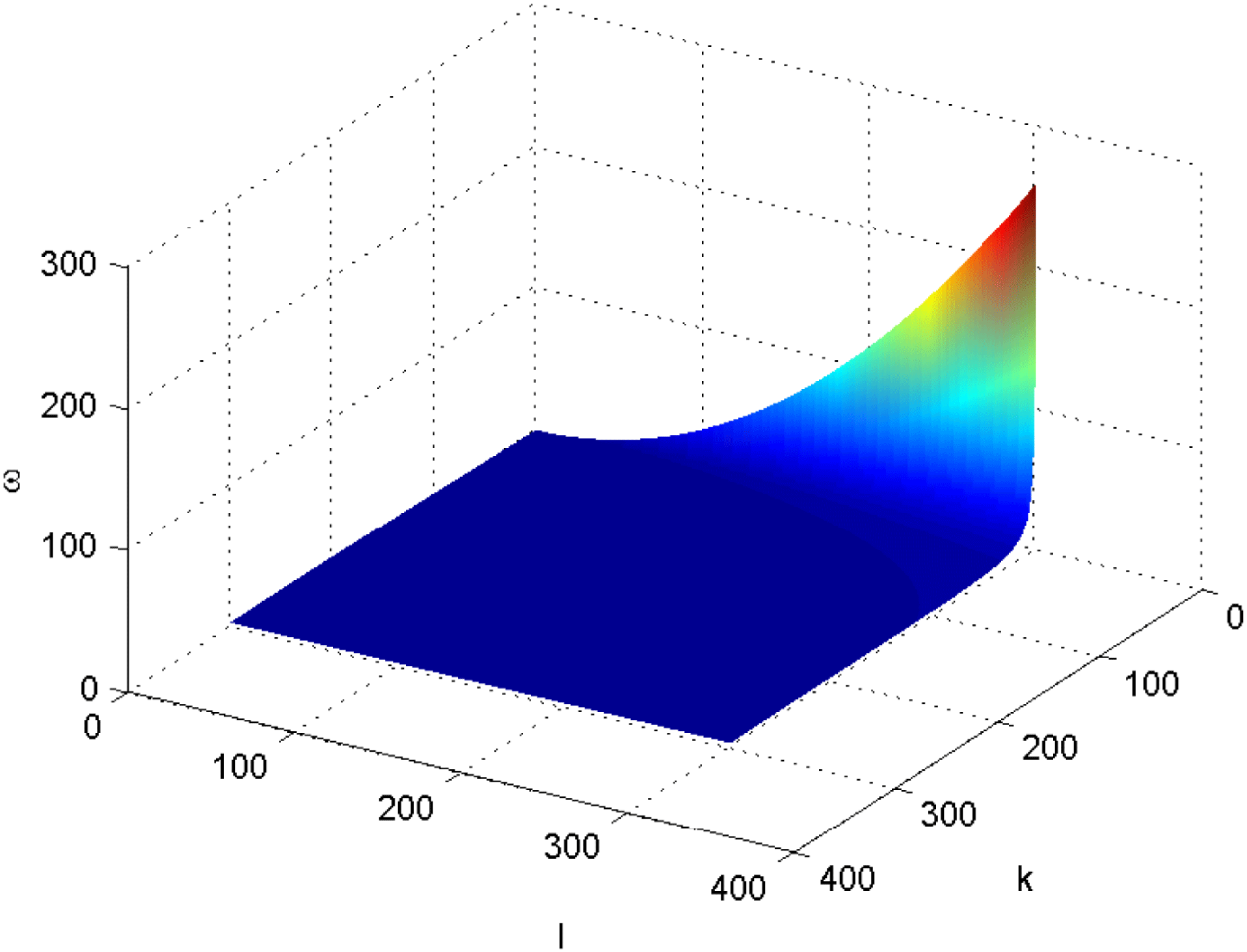
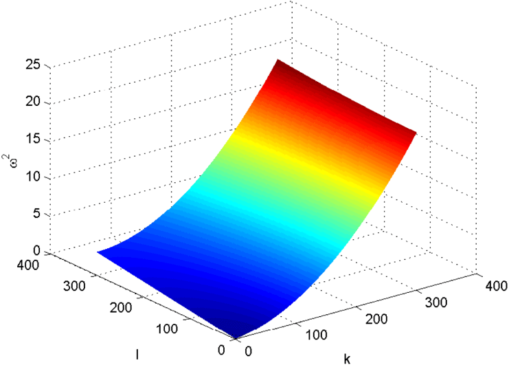
It can be seen, here or in figures 2 and 3 for a graphical solution, that the short waves are only weakly dispersive as
 $\unicode[STIX]{x1D714}\sim \sqrt{M}k+o(k)$
and the
 $\sqrt{k^{2}+l^{2}}$
gives the weak dispersion whereas for the long linear MHD surface waves, there is no dispersion depending on the wave vector for a large part of the domain.
4 Magnetic Kadomtsev–Petviashvili (KP) equation
The linear free surface profile,
 $\unicode[STIX]{x1D702}_{1}(x,y)$
arising from a moving pressure distribution moving with speed
 $U$
say can be computed using the techniques of § 3. One can plot
 $\unicode[STIX]{x1D702}_{1}(x,0)$
against
 $U/U_{m}in$
and see a singularity appear at
 $U/U_{m}in=1$
, see Hunt (Reference Hunt2013, § 2.3.2). Therefore, it is necessary to move to weakly nonlinear theory. The derivation will follow the method laid out by Johnson (Reference Johnson1997). Starting with the equations (2.1)–(2.8), introduce the following scaling
 $$\begin{eqnarray}x=L\hat{x},\quad y=L{\hat{y}},\quad z=h\hat{z},\quad t=\frac{L}{\sqrt{gh}}\hat{t},\quad u=\sqrt{gh}\hat{u} ,\end{eqnarray}$$
 $$\begin{eqnarray}v=\sqrt{gh}\hat{v},\quad w=\frac{h\sqrt{gh}}{L}{\hat{w}},\quad \boldsymbol{B}=B_{0}\hat{\boldsymbol{B}},\quad \unicode[STIX]{x1D702}=a\hat{\unicode[STIX]{x1D702}}.\end{eqnarray}$$
As the perturbations in the free surface are going to be small it follows that there can really be no large quantities. To this end the pressure is scaled
 $p\mapsto \unicode[STIX]{x1D700}p$
in order to obtain a consistent system of equations. The process of choosing the scaling which yields the most terms is often referred to as the principle of least degeneration. In the process of non-dimensionalisation, there are two parameters which appear
 $$\begin{eqnarray}\unicode[STIX]{x1D6FC}=\frac{a}{h},\quad \unicode[STIX]{x1D6FD}=\frac{h^{2}}{L^{2}}.\end{eqnarray}$$
In order to balance the nonlinearity and the dispersion take
 $\unicode[STIX]{x1D6FC}=\unicode[STIX]{x1D6FD}=\unicode[STIX]{x1D700}$
and make the following change of variables, as suggested by Johnson (Reference Johnson1997)
 $$\begin{eqnarray}X=\hat{x}-\hat{t},\quad T=\unicode[STIX]{x1D700}\hat{t},\quad y=\sqrt{\unicode[STIX]{x1D700}}Y,\quad v=\sqrt{\unicode[STIX]{x1D700}}V,\quad M=\unicode[STIX]{x1D700}\bar{M}.\end{eqnarray}$$
Implicitly,
 $M\ll 1$
, which implies that
 $B_{0}^{2}/\unicode[STIX]{x1D707}\unicode[STIX]{x1D70C}\ll gh$
which means that the magnetic field must be small. The equations (2.1)–(2.8) now become
 $$\begin{eqnarray}\displaystyle & \displaystyle \frac{\unicode[STIX]{x2202}u}{\unicode[STIX]{x2202}X}+\unicode[STIX]{x1D700}\frac{\unicode[STIX]{x2202}V}{\unicode[STIX]{x2202}Y}+\frac{\unicode[STIX]{x2202}w}{\unicode[STIX]{x2202}z}=0, & \displaystyle\end{eqnarray}$$
 $$\begin{eqnarray}\displaystyle & \displaystyle \unicode[STIX]{x1D700}\frac{\unicode[STIX]{x2202}u}{\unicode[STIX]{x2202}T}-\unicode[STIX]{x1D700}\frac{\unicode[STIX]{x2202}u}{\unicode[STIX]{x2202}X}+\unicode[STIX]{x1D700}^{2}\left(u\frac{\unicode[STIX]{x2202}u}{\unicode[STIX]{x2202}X}+\unicode[STIX]{x1D700}V\frac{\unicode[STIX]{x2202}u}{\unicode[STIX]{x2202}Y}+w\frac{\unicode[STIX]{x2202}u}{\unicode[STIX]{x2202}z}\right)\qquad \qquad \qquad \qquad & \displaystyle \nonumber\\ \displaystyle & \displaystyle \qquad \qquad =-\frac{\unicode[STIX]{x2202}}{\unicode[STIX]{x2202}X}\left(\unicode[STIX]{x1D700}p+\frac{\unicode[STIX]{x1D700}\bar{M}|\boldsymbol{B}|^{2}}{2}\right)+\unicode[STIX]{x1D700}\bar{M}\left(B_{x}\frac{\unicode[STIX]{x2202}B_{x}}{\unicode[STIX]{x2202}X}+\sqrt{\unicode[STIX]{x1D700}}B_{y}\frac{\unicode[STIX]{x2202}B_{x}}{\unicode[STIX]{x2202}Y}+B_{z}\frac{\unicode[STIX]{x2202}B_{x}}{\unicode[STIX]{x2202}z}\right), & \displaystyle\end{eqnarray}$$
 $$\begin{eqnarray}\displaystyle & \displaystyle \unicode[STIX]{x1D700}^{5/2}\frac{\unicode[STIX]{x2202}v}{\unicode[STIX]{x2202}T}-\unicode[STIX]{x1D700}^{3/2}\frac{\unicode[STIX]{x2202}V}{\unicode[STIX]{x2202}X}+\unicode[STIX]{x1D700}^{5/2}\left(u\frac{\unicode[STIX]{x2202}V}{\unicode[STIX]{x2202}X}+\unicode[STIX]{x1D700}V\frac{\unicode[STIX]{x2202}V}{\unicode[STIX]{x2202}Y}+w\frac{\unicode[STIX]{x2202}V}{\unicode[STIX]{x2202}z}\right)\qquad \qquad \qquad \qquad & \displaystyle \nonumber\\ \displaystyle & \displaystyle \qquad =-\sqrt{\unicode[STIX]{x1D700}}\frac{\unicode[STIX]{x2202}}{\unicode[STIX]{x2202}Y}\left(\unicode[STIX]{x1D700}p+\frac{\unicode[STIX]{x1D700}\bar{M}|\boldsymbol{B}|^{2}}{2}\right)+\unicode[STIX]{x1D700}\bar{M}\left(B_{x}\frac{\unicode[STIX]{x2202}B_{y}}{\unicode[STIX]{x2202}X}+\sqrt{\unicode[STIX]{x1D700}}B_{y}\frac{\unicode[STIX]{x2202}B_{y}}{\unicode[STIX]{x2202}Y}+B_{z}\frac{\unicode[STIX]{x2202}B_{y}}{\unicode[STIX]{x2202}z}\right), & \displaystyle\end{eqnarray}$$
 $$\begin{eqnarray}\displaystyle & \displaystyle \unicode[STIX]{x1D700}^{3}\frac{\unicode[STIX]{x2202}w}{\unicode[STIX]{x2202}T}-\unicode[STIX]{x1D700}^{2}\frac{\unicode[STIX]{x2202}w}{\unicode[STIX]{x2202}X}\left(u\frac{\unicode[STIX]{x2202}w}{\unicode[STIX]{x2202}X}+\sqrt{\unicode[STIX]{x1D700}}V\frac{\unicode[STIX]{x2202}w}{\unicode[STIX]{x2202}Y}+w\frac{\unicode[STIX]{x2202}w}{\unicode[STIX]{x2202}z}\right)\qquad \qquad \qquad \qquad \qquad & \displaystyle \nonumber\\ \displaystyle & \displaystyle \qquad =-\frac{\unicode[STIX]{x2202}}{\unicode[STIX]{x2202}z}\left(\unicode[STIX]{x1D700}p+\frac{\unicode[STIX]{x1D700}\bar{M}|\boldsymbol{B}|^{2}}{2}\right)+\unicode[STIX]{x1D700}\bar{M}\left(B_{x}\frac{\unicode[STIX]{x2202}B_{z}}{\unicode[STIX]{x2202}X}+\unicode[STIX]{x1D700}B_{z}\frac{\unicode[STIX]{x2202}B_{y}}{\unicode[STIX]{x2202}Y}+B_{z}\frac{\unicode[STIX]{x2202}B_{z}}{\unicode[STIX]{x2202}z}\right), & \displaystyle\end{eqnarray}$$
 $$\begin{eqnarray}\displaystyle & \displaystyle \unicode[STIX]{x1D700}\frac{\unicode[STIX]{x2202}B_{x}}{\unicode[STIX]{x2202}T}-\frac{\unicode[STIX]{x2202}B_{x}}{\unicode[STIX]{x2202}X}=\unicode[STIX]{x1D700}^{3/2}\frac{\unicode[STIX]{x2202}}{\unicode[STIX]{x2202}Y}(uB_{y}-\sqrt{\unicode[STIX]{x1D700}}VB_{x})-\sqrt{\unicode[STIX]{x1D700}}\frac{\unicode[STIX]{x2202}}{\unicode[STIX]{x2202}z}(\sqrt{\unicode[STIX]{x1D700}}wB_{x}-uB_{z}), & \displaystyle\end{eqnarray}$$
 $$\begin{eqnarray}\displaystyle & \displaystyle \unicode[STIX]{x1D700}\frac{\unicode[STIX]{x2202}B_{y}}{\unicode[STIX]{x2202}T}-\frac{\unicode[STIX]{x2202}B_{y}}{\unicode[STIX]{x2202}X}=\unicode[STIX]{x1D700}\frac{\unicode[STIX]{x2202}}{\unicode[STIX]{x2202}z}(VB_{z}-wB_{y})-\unicode[STIX]{x1D700}\frac{\unicode[STIX]{x2202}}{\unicode[STIX]{x2202}X}(uB_{y}-\sqrt{\unicode[STIX]{x1D700}}VB_{x}), & \displaystyle\end{eqnarray}$$
 $$\begin{eqnarray}\displaystyle & \displaystyle \unicode[STIX]{x1D700}\frac{\unicode[STIX]{x2202}B_{z}}{\unicode[STIX]{x2202}T}-\frac{\unicode[STIX]{x2202}B_{z}}{\unicode[STIX]{x2202}X}=\unicode[STIX]{x1D700}\frac{\unicode[STIX]{x2202}}{\unicode[STIX]{x2202}z}(\sqrt{\unicode[STIX]{x1D700}}wB_{x}-uB_{z})-\unicode[STIX]{x1D700}^{2}\frac{\unicode[STIX]{x2202}}{\unicode[STIX]{x2202}Y}(VB_{z}-wB_{y}), & \displaystyle\end{eqnarray}$$
 $$\begin{eqnarray}\displaystyle & \displaystyle \frac{\unicode[STIX]{x2202}B_{x}}{\unicode[STIX]{x2202}X}+\sqrt{\unicode[STIX]{x1D700}}\frac{\unicode[STIX]{x2202}B_{y}}{\unicode[STIX]{x2202}Y}+\frac{1}{\sqrt{\unicode[STIX]{x1D700}}}\frac{\unicode[STIX]{x2202}B_{z}}{\unicode[STIX]{x2202}z}=0, & \displaystyle\end{eqnarray}$$
 $$\begin{eqnarray}\displaystyle & \displaystyle \unicode[STIX]{x1D700}p-\unicode[STIX]{x1D700}\unicode[STIX]{x1D702}-\frac{\unicode[STIX]{x1D700}\bar{M}}{2}+\frac{\unicode[STIX]{x1D700}\bar{M}|\boldsymbol{B}|^{2}}{2}=0,\quad z=\unicode[STIX]{x1D700}\unicode[STIX]{x1D702}(T,X,Y), & \displaystyle\end{eqnarray}$$
and
 $$\begin{eqnarray}\unicode[STIX]{x1D700}\frac{\unicode[STIX]{x2202}\unicode[STIX]{x1D702}}{\unicode[STIX]{x2202}T}-\frac{\unicode[STIX]{x2202}\unicode[STIX]{x1D702}}{\unicode[STIX]{x2202}X}+\unicode[STIX]{x1D700}u\frac{\unicode[STIX]{x2202}\unicode[STIX]{x1D702}}{\unicode[STIX]{x2202}X}+\unicode[STIX]{x1D700}^{2}\frac{\unicode[STIX]{x2202}\unicode[STIX]{x1D702}}{\unicode[STIX]{x2202}Y}=w,\quad z=\unicode[STIX]{x1D700}\unicode[STIX]{x1D702}(T,X,Y).\end{eqnarray}$$
The nonlinear governing equations are perturbed as
 $$\begin{eqnarray}\displaystyle & \displaystyle p,u,V,w,\unicode[STIX]{x1D702}=p_{0},u_{0},V_{0},w_{0},\unicode[STIX]{x1D702}_{0}+\unicode[STIX]{x1D700}p_{1},\unicode[STIX]{x1D700}u_{1},\unicode[STIX]{x1D700}V_{1},\unicode[STIX]{x1D700}w_{1},\unicode[STIX]{x1D700}\unicode[STIX]{x1D702}_{1}+o(\unicode[STIX]{x1D700}), & \displaystyle\end{eqnarray}$$
 $$\begin{eqnarray}\displaystyle & \displaystyle B_{x}=1+\unicode[STIX]{x1D700}B_{1x}+\unicode[STIX]{x1D700}^{2}B_{2x}+o(\unicode[STIX]{x1D700}^{2}), & \displaystyle\end{eqnarray}$$
 $$\begin{eqnarray}\displaystyle & \displaystyle B_{y},B_{z}=\unicode[STIX]{x1D700}^{3/2}B_{1y},\unicode[STIX]{x1D700}^{3/2}B_{1z}+o(\unicode[STIX]{x1D700}^{3/2}). & \displaystyle\end{eqnarray}$$
Considering the lowest order
 $O(\unicode[STIX]{x1D700})$
of equations (2.1)–(2.8) equations, we obtain
 $$\begin{eqnarray}\frac{\unicode[STIX]{x2202}u_{0}}{\unicode[STIX]{x2202}X}+\frac{\unicode[STIX]{x2202}w_{0}}{\unicode[STIX]{x2202}Z}=0,\quad \frac{\unicode[STIX]{x2202}u_{0}}{\unicode[STIX]{x2202}X}=\frac{\unicode[STIX]{x2202}p_{0}}{\unicode[STIX]{x2202}X},\quad \frac{\unicode[STIX]{x2202}p_{0}}{\unicode[STIX]{x2202}z}=0,\quad \frac{\unicode[STIX]{x2202}B_{1x}}{\unicode[STIX]{x2202}X}=\frac{\unicode[STIX]{x2202}w_{0}}{\unicode[STIX]{x2202}z},\end{eqnarray}$$
 $$\begin{eqnarray}\frac{\unicode[STIX]{x2202}V_{0}}{\unicode[STIX]{x2202}X}=\frac{\unicode[STIX]{x2202}p_{0}}{\unicode[STIX]{x2202}Y},\quad \frac{\unicode[STIX]{x2202}B_{1y}}{\unicode[STIX]{x2202}X}=\frac{\unicode[STIX]{x2202}V_{0}}{\unicode[STIX]{x2202}X},\quad \frac{\unicode[STIX]{x2202}B_{1z}}{\unicode[STIX]{x2202}X}=\frac{\unicode[STIX]{x2202}w_{0}}{\unicode[STIX]{x2202}X}.\end{eqnarray}$$
The boundary conditions read as
 $$\begin{eqnarray}p_{0}=\unicode[STIX]{x1D702}_{0},\quad w_{0}=-\frac{\unicode[STIX]{x2202}\unicode[STIX]{x1D702}_{0}}{\unicode[STIX]{x2202}X},\quad \text{on }z=0.\end{eqnarray}$$
The solutions of these equations in dimensionless form are
 $$\begin{eqnarray}p_{0}=u_{0}=-B_{1x}=\unicode[STIX]{x1D702}_{0},\quad w_{0}=-(1+z)\frac{\unicode[STIX]{x2202}\unicode[STIX]{x1D702}_{0}}{\unicode[STIX]{x2202}X},\quad \frac{\unicode[STIX]{x2202}V_{0}}{\unicode[STIX]{x2202}X}=\frac{\unicode[STIX]{x2202}\unicode[STIX]{x1D702}_{0}}{\unicode[STIX]{x2202}Y}.\end{eqnarray}$$
The next order equations are straightforward
 $$\begin{eqnarray}\displaystyle & \displaystyle \frac{\unicode[STIX]{x2202}u_{1}}{\unicode[STIX]{x2202}X}+\frac{\unicode[STIX]{x2202}V_{0}}{\unicode[STIX]{x2202}Y}+\frac{\unicode[STIX]{x2202}w_{1}}{\unicode[STIX]{x2202}z}=0, & \displaystyle\end{eqnarray}$$
 $$\begin{eqnarray}\displaystyle & \displaystyle \frac{\unicode[STIX]{x2202}\unicode[STIX]{x1D702}_{0}}{\unicode[STIX]{x2202}T}-\frac{\unicode[STIX]{x2202}u_{1}}{\unicode[STIX]{x2202}X}+\unicode[STIX]{x1D702}_{0}\frac{\unicode[STIX]{x2202}\unicode[STIX]{x1D702}_{0}}{\unicode[STIX]{x2202}X}=-\frac{\unicode[STIX]{x2202}p_{1}}{\unicode[STIX]{x2202}X}, & \displaystyle\end{eqnarray}$$
 $$\begin{eqnarray}\displaystyle & \displaystyle -(z+1)\frac{\unicode[STIX]{x2202}^{2}\unicode[STIX]{x1D702}_{0}}{\unicode[STIX]{x2202}X^{2}}=\frac{\unicode[STIX]{x2202}p_{1}}{\unicode[STIX]{x2202}z}. & \displaystyle\end{eqnarray}$$
Along with the boundary conditions
 $$\begin{eqnarray}p_{1}+\bar{M}B_{1x}=\unicode[STIX]{x1D702}_{1},\quad \frac{\unicode[STIX]{x2202}\unicode[STIX]{x1D702}_{0}}{\unicode[STIX]{x2202}T}-\frac{\unicode[STIX]{x2202}\unicode[STIX]{x1D702}_{1}}{\unicode[STIX]{x2202}X}+2\unicode[STIX]{x1D702}_{0}\frac{\unicode[STIX]{x2202}\unicode[STIX]{x1D702}_{0}}{\unicode[STIX]{x2202}X}=w_{1}.\end{eqnarray}$$
Integrating (4.24) and using the first equation of (4.25) shows that
 $$\begin{eqnarray}p_{1}=\frac{1}{2}\left[1-(1+z)^{2}\right]\frac{\unicode[STIX]{x2202}^{2}\unicode[STIX]{x1D702}_{0}}{\unicode[STIX]{x2202}X^{2}}+\unicode[STIX]{x1D702}_{1}+\bar{M}\unicode[STIX]{x1D702}_{0}.\end{eqnarray}$$
To find
 $w_{1}$
, insert (4.26) into (4.23), substitute
 $\unicode[STIX]{x2202}_{X}u_{1}$
into (4.22), and, integrate it with respect to
 $z$
to have
 $$\begin{eqnarray}w_{1}=-\frac{1}{3}\frac{\unicode[STIX]{x2202}^{3}\unicode[STIX]{x1D702}_{0}}{\unicode[STIX]{x2202}X^{3}}-\frac{\unicode[STIX]{x2202}\unicode[STIX]{x1D702}_{1}}{\unicode[STIX]{x2202}X}+\unicode[STIX]{x1D702}_{0}\frac{\unicode[STIX]{x2202}\unicode[STIX]{x1D702}_{0}}{\unicode[STIX]{x2202}X}-\bar{M}\frac{\unicode[STIX]{x2202}\unicode[STIX]{x1D702}_{0}}{\unicode[STIX]{x2202}X}-\frac{\unicode[STIX]{x2202}\unicode[STIX]{x1D702}_{0}}{\unicode[STIX]{x2202}T}-\frac{\unicode[STIX]{x2202}V_{0}}{\unicode[STIX]{x2202}Y}.\end{eqnarray}$$
The appearance of the
 $\unicode[STIX]{x2202}_{X}^{3}\unicode[STIX]{x1D702}_{0}$
term shows why the
 $k^{4}$
term must be kept in the dispersion relation. Inserting (4.27) into the second equation of (4.25) and differentiating with respect to
 $X$
gives
 $$\begin{eqnarray}\frac{\unicode[STIX]{x2202}}{\unicode[STIX]{x2202}X}\left[\frac{\unicode[STIX]{x2202}\unicode[STIX]{x1D702}_{0}}{\unicode[STIX]{x2202}T}+\frac{3}{2}\unicode[STIX]{x1D702}_{0}\frac{\unicode[STIX]{x2202}\unicode[STIX]{x1D702}_{0}}{\unicode[STIX]{x2202}X}+\frac{\bar{M}}{2}\frac{\unicode[STIX]{x2202}\unicode[STIX]{x1D702}_{0}}{\unicode[STIX]{x2202}X}+\frac{1}{6}\frac{\unicode[STIX]{x2202}^{3}\unicode[STIX]{x1D702}_{0}}{\unicode[STIX]{x2202}X^{3}}\right]+\frac{1}{2}\frac{\unicode[STIX]{x2202}^{2}\unicode[STIX]{x1D702}_{0}}{\unicode[STIX]{x2202}Y^{2}}=0.\end{eqnarray}$$
It may be noted that a coordinate transformation may remove the term
 $\bar{M}\unicode[STIX]{x2202}_{X}\unicode[STIX]{x1D702}_{0}/2$
. This term may be regarded as setting the correct wave speed. After applying the coordinate transformation (4.28) reduces to the well-known Kadomtsev–Petviashvili equation. This is done by moving back into the scaled coordinates defined by
 $$\begin{eqnarray}X=\hat{x}-\hat{t},\quad T=\unicode[STIX]{x1D700}\hat{t},\quad Y=\frac{{\hat{y}}}{\sqrt{\unicode[STIX]{x1D700}}}.\end{eqnarray}$$
KP is known to be integrable and has analytical solutions (Johnson Reference Johnson1997). From these solutions of the KP equation one can now obtain solutions to (4.28) via coordinate transformation.
5 Magnetic fields in both regions
Consider now the problem described in § 1 with a magnetic field in both regions. Region 1 is defined by
 $\{(x,y,z)|z>\unicode[STIX]{x1D702}(t,x,y,z)\}$
, and, region 2 is defined by
 $\{(x,y,z)|-h\leqslant z\leqslant \unicode[STIX]{x1D702}(t,x,y,z)\}$
. There is no current in region 2, and so
 $\unicode[STIX]{x1D735}\times \boldsymbol{B}_{2}=\mathbf{0}$
, i.e. it can be stated that
 $\boldsymbol{B}_{2}=\unicode[STIX]{x1D735}\unicode[STIX]{x1D6F7}$
. The two boundary conditions which must be obeyed are
 $$\begin{eqnarray}\displaystyle & \displaystyle \boldsymbol{B}_{2}\rightarrow \boldsymbol{B}_{2,0}\quad \text{as }z\rightarrow \infty & \displaystyle\end{eqnarray}$$
 $$\begin{eqnarray}\displaystyle & \displaystyle \boldsymbol{B}_{2}\boldsymbol{\cdot }\hat{\boldsymbol{n}}=0\quad z=\unicode[STIX]{x1D702}(t,x,y). & \displaystyle\end{eqnarray}$$
The magnetic field in region 2 can be written in the following manner
 $$\begin{eqnarray}\boldsymbol{B}_{2}=\boldsymbol{B}_{2,0}+\unicode[STIX]{x1D735}\unicode[STIX]{x1D6F7}\end{eqnarray}$$
to yield the equation:
 $$\begin{eqnarray}\unicode[STIX]{x1D6FB}^{2}\unicode[STIX]{x1D6F7}=0.\end{eqnarray}$$
One of the boundary conditions which links the magnetic field in region 1 to the magnetic field of region 2 is
 $$\begin{eqnarray}\left[p+\frac{|\boldsymbol{B}|^{2}}{2\unicode[STIX]{x1D707}}\right]_{1}^{2}=0.\end{eqnarray}$$
The boundary condition
 $\boldsymbol{B}\boldsymbol{\cdot }\hat{\boldsymbol{n}}=0$
reduces to the following
 $$\begin{eqnarray}\boldsymbol{B}_{1,0}\boldsymbol{\cdot }\boldsymbol{e}_{x}\unicode[STIX]{x2202}_{x}\unicode[STIX]{x1D702}=\boldsymbol{B}_{1,0}\boldsymbol{\cdot }\boldsymbol{e}_{z},\end{eqnarray}$$
yielding a lower boundary condition.
5.1 Linear theory
5.1.1 Derivation of dispersion relation
A dispersion relation is sought to gain insight into how waves will propagate in a magnetised fluid system. The derivation is very similar to the previous case with the magnetic field confined to the fluid. The equilibrium condition for the magnetic field in region
 $1$
is given by
 $\boldsymbol{B}=B_{1}\boldsymbol{e}_{x}$
. The scaling for the linear case is the same as in the previous case in § 3. The magnetic field in region
 $1$
is scaled as
 $\boldsymbol{B}=B_{1}\hat{\boldsymbol{B}}$
. The equilibrium pressure, in this case, is determined as before. The general kinetic pressure is
 $p=-\unicode[STIX]{x1D70C}_{0}gz+C$
. The continuity of total pressure now reads
 $$\begin{eqnarray}p(0)+\frac{B_{1,0}^{2}}{2\unicode[STIX]{x1D707}_{1}}=p_{a}+\frac{B_{2,0}^{2}}{2\unicode[STIX]{x1D707}_{2}}.\end{eqnarray}$$
The scaled equations are then
 $$\begin{eqnarray}\displaystyle & \displaystyle \frac{\text{D}\hat{\boldsymbol{u}}}{\text{D}\hat{t}}=-\hat{\unicode[STIX]{x1D735}}\left(\hat{p}+\frac{M_{2}|\hat{\boldsymbol{B}_{2}}|^{2}}{2}\right)+M_{2}(\hat{\boldsymbol{B}_{2}}\boldsymbol{\cdot }\hat{\unicode[STIX]{x1D735}})\hat{\boldsymbol{B}_{2}},\quad -1\leqslant \hat{z}\leqslant \hat{\unicode[STIX]{x1D702}}(\hat{t},\hat{x},{\hat{y}}), & \displaystyle\end{eqnarray}$$
 $$\begin{eqnarray}\displaystyle & \displaystyle \frac{\text{D}\hat{\boldsymbol{B}}_{2}}{\text{D}\hat{t}}=(\hat{\boldsymbol{B}}_{2}\boldsymbol{\cdot }\hat{\unicode[STIX]{x1D735}})\hat{\boldsymbol{u}},\quad -1\leqslant \hat{z}\leqslant \hat{\unicode[STIX]{x1D702}}(\hat{t},\hat{x},{\hat{y}}), & \displaystyle\end{eqnarray}$$
 $$\begin{eqnarray}\displaystyle & \displaystyle \hat{\unicode[STIX]{x1D735}}\boldsymbol{\cdot }\hat{\boldsymbol{u}}=0,\quad -1\leqslant \hat{z}\leqslant \hat{\unicode[STIX]{x1D702}}(\hat{t},\hat{x},{\hat{y}}), & \displaystyle\end{eqnarray}$$
 $$\begin{eqnarray}\displaystyle & \displaystyle \hat{\unicode[STIX]{x1D735}}\boldsymbol{\cdot }\hat{\boldsymbol{B}}_{2}=0,\quad -1\leqslant \hat{z}\leqslant \hat{\unicode[STIX]{x1D702}}(\hat{t},\hat{x},{\hat{y}}), & \displaystyle\end{eqnarray}$$
 $$\begin{eqnarray}\displaystyle & \displaystyle \unicode[STIX]{x1D6FB}^{2}\hat{\unicode[STIX]{x1D6F7}}=0,\quad \hat{\unicode[STIX]{x1D702}}(\hat{t},\hat{x},{\hat{y}})<\hat{z}<\infty , & \displaystyle\end{eqnarray}$$
 $$\begin{eqnarray}\displaystyle & \displaystyle \frac{\unicode[STIX]{x2202}\hat{\unicode[STIX]{x1D702}}}{\unicode[STIX]{x2202}\hat{t}}+\hat{u} \frac{\unicode[STIX]{x2202}\hat{\unicode[STIX]{x1D702}}}{\unicode[STIX]{x2202}\hat{x}}+v\frac{\unicode[STIX]{x2202}\hat{\unicode[STIX]{x1D702}}}{\unicode[STIX]{x2202}{\hat{y}}}={\hat{w}}\quad \text{on }\hat{z}=\hat{\unicode[STIX]{x1D702}}(\hat{t},\hat{x},{\hat{y}}), & \displaystyle\end{eqnarray}$$
 $$\begin{eqnarray}\displaystyle & \displaystyle \left[\hat{p}-\hat{\unicode[STIX]{x1D702}}+\frac{M|\hat{\boldsymbol{B}}|^{2}}{2}\right]_{1}^{2}=0\quad \text{on }\hat{z}=\hat{\unicode[STIX]{x1D702}}(\hat{t},\hat{x},{\hat{y}}). & \displaystyle\end{eqnarray}$$
 $$\begin{eqnarray}\displaystyle & \displaystyle \hat{B}_{z}=0\quad \text{on }\hat{z}=-1, & \displaystyle\end{eqnarray}$$
 $$\begin{eqnarray}\displaystyle & \displaystyle {\hat{w}}=0\quad \text{on }\hat{z}=-1, & \displaystyle\end{eqnarray}$$
 $$\begin{eqnarray}\displaystyle & \displaystyle \frac{\unicode[STIX]{x2202}_{\hat{x}}\unicode[STIX]{x1D702}}{\sqrt{1+(\unicode[STIX]{x2202}_{\hat{x}}\hat{\unicode[STIX]{x1D702}})^{2}}}=\hat{B}_{1z}\quad \text{on }\hat{z}=\hat{\unicode[STIX]{x1D702}}(\hat{t},\hat{x},{\hat{y}}). & \displaystyle\end{eqnarray}$$
The notation used here is
 $$\begin{eqnarray}M_{1}=\frac{B_{1}^{2}}{gh\unicode[STIX]{x1D707}_{1}\unicode[STIX]{x1D70C}_{2}},\quad M_{2}=\frac{B_{2}^{2}}{gh\unicode[STIX]{x1D707}_{2}\unicode[STIX]{x1D70C}_{2}}.\end{eqnarray}$$
Note that in region 2 the magnetic field scales as the following:
 $$\begin{eqnarray}\hat{\boldsymbol{B}}_{2}=1+\unicode[STIX]{x1D700}\unicode[STIX]{x1D735}\hat{\unicode[STIX]{x1D6F7}},\end{eqnarray}$$
where the variation from the constant field should not be large. The linearisation is now analogous to the previous case in § 3. The no flux condition reduces to
 $$\begin{eqnarray}\hat{\boldsymbol{B}}_{1z}=\unicode[STIX]{x2202}_{x}\unicode[STIX]{x1D702}=\hat{\boldsymbol{B}}_{2z}.\end{eqnarray}$$
which is equivalent to
 $$\begin{eqnarray}B_{1z}=B_{2z}\quad \text{on }\hat{z}=\hat{\unicode[STIX]{x1D702}}(\hat{t},\hat{x},{\hat{y}}).\end{eqnarray}$$
Again, it is assumed the perturbations can be expanded as Fourier transforms and an equation for
 $B_{1z}$
is found which is mathematically similar to that found previously (3.29). Finally, the corresponding dispersion relation is then
 $$\begin{eqnarray}\unicode[STIX]{x1D714}^{2}=M_{2}k^{2}+|\boldsymbol{k}|\tanh |\boldsymbol{k}|+M_{1}k^{2}\tanh |\boldsymbol{k}|.\end{eqnarray}$$
The long wave approximation of the dispersion relation is
 $$\begin{eqnarray}\unicode[STIX]{x1D714}k=\left(1+\frac{M_{2}}{2}\right)k^{2}+\frac{l^{2}}{2}-\frac{k^{4}}{6}+M_{1}k^{2}|k|.\end{eqnarray}$$
Note that this dispersion relation is only valid when
 $M_{1}\ll 1$
, as otherwise it can be ignored. The requirement that
 $M_{2}\ll 1$
was required for mathematical consistency. To obtain a result where
 $M_{1},M_{2}\not \ll 1$
would require different techniques employed in this paper. The approach taken here for the small magnetic field is analogous to the assumption of small surface tension in Benjamin (Reference Benjamin1992). This dispersion relation has appeared several times in the literature before. The first was in Kim & Akylas (Reference Kim and Akylas2006) and the second was in Hunt (Reference Hunt2013). The form of the equations is exactly the same but the coefficients are different, reflecting the application. Upon using the substitutions
 $\unicode[STIX]{x1D714}\mapsto -\text{i}\unicode[STIX]{x2202}_{t},k\mapsto \text{i}\unicode[STIX]{x2202}_{x},l\mapsto \text{i}\unicode[STIX]{x2202}_{y}$
as before, the following linear PDE is obtained governing long-wavelength linear MHD waves propagating along a contact discontinuity in magnetised plasma
 $$\begin{eqnarray}\frac{\unicode[STIX]{x2202}}{\unicode[STIX]{x2202}x}\left[\frac{\unicode[STIX]{x2202}\unicode[STIX]{x1D702}}{\unicode[STIX]{x2202}t}+\left(1+\frac{M_{2}}{2}\right)\frac{\unicode[STIX]{x2202}\unicode[STIX]{x1D702}}{\unicode[STIX]{x2202}x}+\frac{1}{6}\frac{\unicode[STIX]{x2202}^{3}\unicode[STIX]{x1D702}}{\unicode[STIX]{x2202}x^{3}}+M_{1}\mathscr{H}\left(\frac{\unicode[STIX]{x2202}^{2}\unicode[STIX]{x1D702}}{\unicode[STIX]{x2202}x^{2}}\right)\right]+\frac{1}{2}\frac{\unicode[STIX]{x2202}^{2}\unicode[STIX]{x1D702}}{\unicode[STIX]{x2202}y^{2}}=0.\end{eqnarray}$$
This equation represents the linear part to the weakly nonlinear equation in the small amplitude and long wavelength. The nonlinear part of the equation is derived in § 4.
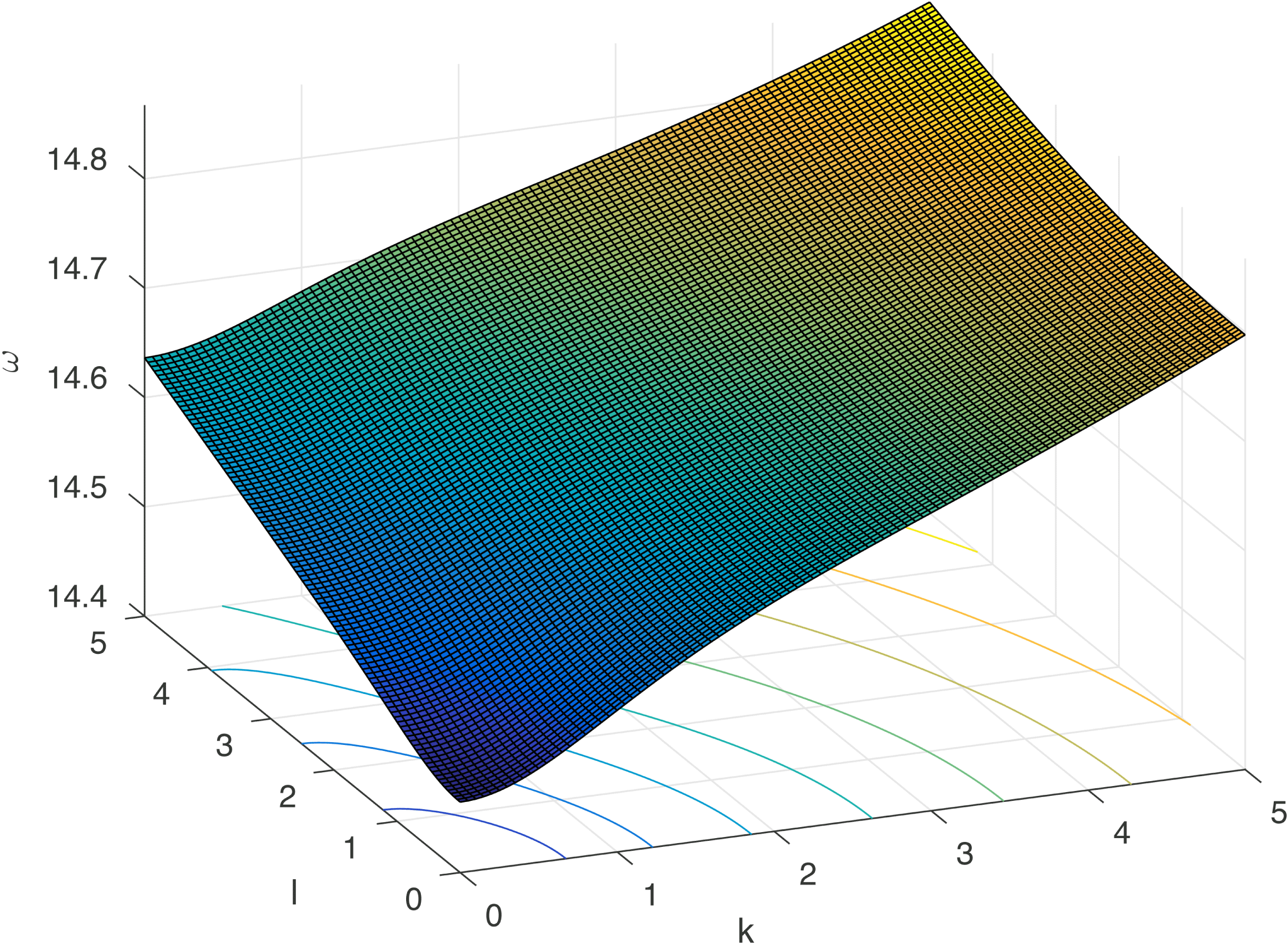
Dispersion relation for infinite
 $\unicode[STIX]{x1D6FD}$
.

5.1.2 Wave profiles from a moving pressure distribution
This section demonstrates a linear two-dimensional wave with a moving pressure distribution to give an idea of some of the linear wave profiles. It is possible to obtain wave profiles for steady linear waves by the use of a moving pressure distribution,
 $P(x,y)$
on the surface of the plasma. In order to do this move to a frame where the plasma is moving uniformly with a velocity
 $\boldsymbol{u}=U\boldsymbol{e}_{x}$
. The scaling for the linear theory is just the same as in § 3 given by (3.6)–(3.7) and as a result the scaled velocity is perturbed from
 $F=U/\sqrt{gh}$
. The linearised governing equations become
 $$\begin{eqnarray}\displaystyle & \displaystyle F\frac{\unicode[STIX]{x2202}\boldsymbol{u}_{1}}{\unicode[STIX]{x2202}x}=-\unicode[STIX]{x1D735}(p_{1}+M_{2}B_{2x})+M_{2}\frac{\unicode[STIX]{x2202}\boldsymbol{B}_{2}}{\unicode[STIX]{x2202}x}, & \displaystyle\end{eqnarray}$$
 $$\begin{eqnarray}\displaystyle & \displaystyle F\frac{\unicode[STIX]{x2202}\boldsymbol{B}_{2}}{\unicode[STIX]{x2202}x}=\frac{\unicode[STIX]{x2202}\boldsymbol{u}_{2}}{\unicode[STIX]{x2202}x}, & \displaystyle\end{eqnarray}$$
 $$\begin{eqnarray}\displaystyle & \displaystyle \unicode[STIX]{x1D735}\boldsymbol{\cdot }\boldsymbol{B}_{2}=0, & \displaystyle\end{eqnarray}$$
 $$\begin{eqnarray}\displaystyle & \displaystyle \unicode[STIX]{x1D735}\boldsymbol{\cdot }\boldsymbol{u}_{2}=0, & \displaystyle\end{eqnarray}$$
 $$\begin{eqnarray}\displaystyle & \displaystyle F\frac{\unicode[STIX]{x2202}\unicode[STIX]{x1D702}_{1}}{\unicode[STIX]{x2202}x}=u_{1z}\quad \text{on }z=0, & \displaystyle\end{eqnarray}$$
 $$\begin{eqnarray}\displaystyle & \displaystyle p_{1}-\unicode[STIX]{x1D702}_{1}+M_{2}B_{2x}=\hat{P}+M_{1}B_{1x}\quad \text{on }z=0, & \displaystyle\end{eqnarray}$$
 $$\begin{eqnarray}\displaystyle & \displaystyle B_{2z}=0\quad \text{on }z=-1, & \displaystyle\end{eqnarray}$$
 $$\begin{eqnarray}\displaystyle & \displaystyle w_{1}=0\quad \text{on }z=-1, & \displaystyle\end{eqnarray}$$
 $$\begin{eqnarray}\displaystyle & \displaystyle B_{1z}=B_{2z}\quad \text{on }z=0. & \displaystyle\end{eqnarray}$$
Following the previous linear calculations given in § 3, an equation is now derived for the
 $z$
-component of the magnetic field equation (3.29). From the solution of (3.29) all other variables can be easily obtained. Finally, in terms of the moving pressure on the surface, the Fourier transform for the free surface is
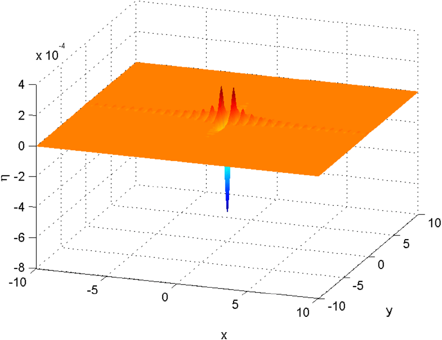
 $$\begin{eqnarray}\hat{\unicode[STIX]{x1D702}}=\frac{|\boldsymbol{k}|\hat{P}}{(F^{2}k^{2}-M_{2}k^{2})\coth (|\boldsymbol{k}|)+|\boldsymbol{k}|(M_{1}k^{2}-1))}.\end{eqnarray}$$
There is an interesting feature of figure 5 in the number of ripples in the wave, which is suggestive that the decay is algebraic. It can be shown that increasing the Froude number to the minimum of the dispersion relation, the amplitude becomes unbounded which is why the need for weakly nonlinear theory.
Travelling linear wave,
 $F=1,M_{2}=1,M_{1}=2$
.

5.2 Weakly nonlinear theory
Consider weakly nonlinear theory of MHD surface wave propagation in the equilibrium defined by (figure 1). Scale the magnetic fields in the following way, following Johnson (Reference Johnson1997):
 $\boldsymbol{B}_{1}=B_{10}\hat{\boldsymbol{B}}_{1}$
and
 $\boldsymbol{B}_{2}=B_{20}\hat{\boldsymbol{B}}_{2}$
. Expand the pressure in region
 $1$
as
 $$\begin{eqnarray}p=p_{a}-\unicode[STIX]{x1D70C}_{0}gz-\frac{B_{10}^{2}}{2\unicode[STIX]{x1D707}_{1}}+\frac{B_{20}^{2}}{2\unicode[STIX]{x1D707}_{2}}+\unicode[STIX]{x1D70C}_{0}gh\hat{p}.\end{eqnarray}$$
The total pressure becomes
 $$\begin{eqnarray}p+C-\unicode[STIX]{x1D700}\hat{\unicode[STIX]{x1D702}}+\frac{M_{1}\hat{|\boldsymbol{B}}_{1}|^{2}}{2}=\frac{M_{2}|\hat{\boldsymbol{B}}_{2}|^{2}}{2},\end{eqnarray}$$
where
 $M_{1,2}=v_{A1,2}^{2}/gh$
. Here
 $v_{A1,2}=B_{1,20}^{2}/2\unicode[STIX]{x1D70C}\unicode[STIX]{x1D707}_{1,2}$
. The transformation
 $p\mapsto \unicode[STIX]{x1D700}p$
is used. For brevity, drop again the hats and set
 $M_{1,2}=\unicode[STIX]{x1D700}\bar{M}_{1,2}$
resulting in
 $$\begin{eqnarray}\unicode[STIX]{x1D700}p-\unicode[STIX]{x1D700}\unicode[STIX]{x1D702}+\frac{\unicode[STIX]{x1D700}\bar{M}_{1}|\boldsymbol{B}_{1}|^{2}}{2}=\frac{\unicode[STIX]{x1D700}\bar{M}_{2}|\boldsymbol{B}_{2}|^{2}}{2}.\end{eqnarray}$$
The governing equation for the magnetic field in region
 $1$
becomes
 $$\begin{eqnarray}\frac{\unicode[STIX]{x2202}^{2}\unicode[STIX]{x1D6F7}}{\unicode[STIX]{x2202}X^{2}}+\unicode[STIX]{x1D700}\frac{\unicode[STIX]{x2202}^{2}\unicode[STIX]{x1D6F7}}{\unicode[STIX]{x2202}Y^{2}}+\frac{\unicode[STIX]{x2202}^{2}\unicode[STIX]{x1D6F7}}{\unicode[STIX]{x2202}z^{2}}=0.\end{eqnarray}$$
This reduces the equation into a two-dimensional Laplace equation, differentiating with respect to
 $z$
yields a Laplace equation for
 $B_{1z}$
, with lower boundary condition
 $B_{1z}(z=0)=\unicode[STIX]{x2202}_{x}\unicode[STIX]{x1D702}$
. The solution for this problem is
 $$\begin{eqnarray}B_{1z}=\frac{1}{\unicode[STIX]{x03C0}}\int _{\mathbb{R}}\frac{z\unicode[STIX]{x2202}_{X}\unicode[STIX]{x1D702}}{(X-X^{\prime })^{2}+z^{2}}\,\text{d}X^{\prime }.\end{eqnarray}$$
To find
 $B_{1X}$
, one integrates with respect to
 $z$
and then differentiates with respect to
 $X$
and then sets
 $z=0$
to obtain
 $$\begin{eqnarray}B_{1X}(z=0)=-\mathscr{H}(\unicode[STIX]{x2202}_{X}\unicode[STIX]{x1D702}).\end{eqnarray}$$
Differentiating the above with respect to
 $X$
and inserting it in equation (4.19), followed by setting
 $z=0$
, shows that
 $$\begin{eqnarray}\frac{\unicode[STIX]{x2202}B_{1X}}{\unicode[STIX]{x2202}X}=\mathscr{H}\left(\frac{\unicode[STIX]{x2202}^{2}\unicode[STIX]{x1D702}_{0}}{\unicode[STIX]{x2202}X^{2}}\right).\end{eqnarray}$$
Just as in § 4, perturbation of the constant magnetic field in the
 $\boldsymbol{e}_{x}$
-direction is introduced. Expand as
 $$\begin{eqnarray}\displaystyle & \displaystyle p=p_{0}+\unicode[STIX]{x1D700}p_{1}+o(\unicode[STIX]{x1D700}), & \displaystyle\end{eqnarray}$$
 $$\begin{eqnarray}\displaystyle & \displaystyle \unicode[STIX]{x1D702}=\unicode[STIX]{x1D702}_{0}+\unicode[STIX]{x1D700}\unicode[STIX]{x1D702}_{1}+o(\unicode[STIX]{x1D700}), & \displaystyle\end{eqnarray}$$
 $$\begin{eqnarray}\displaystyle & \displaystyle B_{1x,2x}=1+\unicode[STIX]{x1D700}B_{1x1,2x1}+o(\unicode[STIX]{x1D700}). & \displaystyle\end{eqnarray}$$
Gathering the expanded terms results in
 $$\begin{eqnarray}\unicode[STIX]{x1D700}(p_{0}+\unicode[STIX]{x1D700}p_{1})-\unicode[STIX]{x1D700}(\unicode[STIX]{x1D702}_{0}+\unicode[STIX]{x1D700}\unicode[STIX]{x1D702}_{1})+\frac{\unicode[STIX]{x1D700}\bar{M}_{1}}{2}(1+2\unicode[STIX]{x1D700}B_{1x1})=\frac{\unicode[STIX]{x1D700}\bar{M}_{2}}{2}(1+2\unicode[STIX]{x1D700}B_{2x1}).\end{eqnarray}$$
The part of this equation with
 $O(\unicode[STIX]{x1D700})$
is
 $$\begin{eqnarray}p_{0}-\unicode[STIX]{x1D702}_{0}=0.\end{eqnarray}$$
The next order,
 $O(\unicode[STIX]{x1D700}^{2})$
, is
 $$\begin{eqnarray}p_{1}-\unicode[STIX]{x1D702}_{1}+\bar{M}_{1}B_{1x1}=\bar{M}_{2x1}.\end{eqnarray}$$
From this point onwards a mathematically analogous analysis can be carried out as in the one-field case (see § 4). The final governing equation is
 $$\begin{eqnarray}\frac{\unicode[STIX]{x2202}}{\unicode[STIX]{x2202}X}\left[\frac{\unicode[STIX]{x2202}\unicode[STIX]{x1D702}_{0}}{\unicode[STIX]{x2202}T}+\frac{\bar{M}_{1}}{2}\frac{\unicode[STIX]{x2202}\unicode[STIX]{x1D702}_{0}}{\unicode[STIX]{x2202}X}+\frac{3}{2}\unicode[STIX]{x1D702}_{0}\frac{\unicode[STIX]{x2202}\unicode[STIX]{x1D702}_{0}}{\unicode[STIX]{x2202}X}+\frac{1}{2}\frac{\unicode[STIX]{x2202}^{3}\unicode[STIX]{x1D702}_{0}}{\unicode[STIX]{x2202}X^{3}}+\frac{\bar{M}_{2}}{2}\mathscr{H}\left(\frac{\unicode[STIX]{x2202}^{2}\unicode[STIX]{x1D702}_{0}}{\unicode[STIX]{x2202}X^{2}}\right)\right]+\frac{1}{2}\frac{\unicode[STIX]{x2202}^{2}\unicode[STIX]{x1D702}_{0}}{\unicode[STIX]{x2202}Y^{2}}=0.\end{eqnarray}$$
The one-dimensional version of this equation, known as the Benjamin equation, was derived in Benjamin (Reference Benjamin1992) using a different method than the one used here. The two-dimensional Benjamin equation has appeared in several instances, in interfacial flows examined in Kim & Akylas (Reference Kim and Akylas2006) and in electrohydrodynamics (Hunt Reference Hunt, Vanden-Broeck, Papageorgiou and Parau2017).
6 Discussion and conclusions
The new result presented in this paper is the derivation of an equation that describes the weakly nonlinear wave propagation in
 $2+1$
dimensions. The equation has been investigated elsewhere in different circumstances. Nevertheless, some important results have been found by other authors. In Zaiter (Reference Zaiter2009), the author proves the existence of solutions of (5.48) as well as the algebraic decay of solutions. In Kim & Akylas (Reference Kim and Akylas2006), they study bifurcation of steady lump solutions and also prove instability results concerning transverse stability. As of writing, there are no known analytical solutions to the one-dimensional Benjamin equation.
A numerical solution of the Benjamin equation would provide valuable insight but that is not within the scope of the present paper.
Acknowledgement
I would like to thank Professor R. Erdélyi for his helpful comments for this work.