

1 Introduction
In this paper we extend our earlier work on the two-dimensional shallow-water system described in Thomas, Buhler & Smith (Reference Thomas, Buhler and Smith2018, hereafter Reference Thomas, Buhler and SmithTBS18) to the significantly more complicated case of the three-dimensional Boussinesq system. Here, as there, our motivation is to develop the theoretical underpinnings of wave-induced particle motions for parameters of relevance to oceanic regimes where simplistic textbook conceptions of a clear distinction between balanced quasi-geostrophic flows and unbalanced waves break down. Following the injection of near-inertial energy by storms, for example, the amplitude of the wave motions can match or exceed that of the balanced mesoscale flow, possibly leading to stronger interactions between the waves and the balanced flow, and to a competition as to which part of the flow dominates the irreversible displacement of fluid particles at different scales (we refer to Reference Thomas, Buhler and SmithTBS18 for a further discussion of relevant ocean dynamics and for citations of recent work on related topics).
We focus here on second-order fluid motion induced solely by linear inertia–gravity waves, a setting that can be made precise by demanding that the potential vorticity (PV) is equal to its uniform background value everywhere and at all times. This leaves wide leeway for the choice of suitable wave fields to consider. For example, Bühler & Holmes-Cerfon (Reference Bühler and Holmes-Cerfon2009), Holmes-Cerfon, Bühler & Ferrari (Reference Holmes-Cerfon, Bühler and Ferrari2011) and Bühler, Grisouard & Holmes-Cerfon (Reference Bühler, Grisouard and Holmes-Cerfon2013) computed the particle diffusion induced by Gaussian random waves, which feature statistically independent Fourier modes. This is essentially a bath of random waves, an extreme model for highly disorganized broadband wave spectra. Conversely, the consideration of mean-flow responses to slowly varying wavetrains or individual wavepackets provides another conceptual bookend to the range of possible choices for the wave field, this time by focusing on narrowband and deterministic wave fields.
In geophysical fluid dynamics the study of mean-flow responses due to packets of internal waves started with the seminal work by Bretherton (Reference Bretherton1969, hereafter Reference BrethertonB69), who computed the second-order mean-flow response in an unbounded domain due to three-dimensional or two-dimensional packets of internal waves in non-rotating flows (i.e. the Coriolis parameter  $f=0$ in these cases). In the three-dimensional case he found a co-moving solution (i.e. a solution that is steady in the frame moving with the wavepacket), which consisted of a layerwise dipolar horizontal return flow on all the stratification surfaces currently intersected by the wavepacket. This ‘Bretherton flow’ was maximal at the centre of the wavepacket (and proportional to the strength of the horizontal pseudomomentum there) and decayed algebraically with horizontal distance from the wavepacket. In stark contrast to the three-dimensional case, the mean-flow response to a two-dimensional wavepacket in the vertical plane turned out not to be a co-moving solution, but rather consisted of persistent radiation of waves at second order in wave amplitude. McIntyre (Reference McIntyre1973) followed up on this work, adapting Bretherton’s unbounded two-dimensional case to a one-dimensional horizontal waveguide with vertically confining boundaries at
 $z=0$ and
 $z=H$, which significantly altered the mean-flow response and raised subtle questions about the ultimate limitations of being able to attribute a well-defined momentum to wavepackets.
The scope of the problem was widened considerably by Grimshaw (Reference Grimshaw1975), who considered general three-dimensional rotating flows and highlighted for the first time that the wave-induced quadratic forcing terms in the mean-flow equations could sometimes be interpreted as ‘generation of PV by the waves’, an idea that would gain significant traction in the sequel. This idea was independently investigated further by Bühler & McIntyre (Reference Bühler and McIntyre1998), who extended Reference BrethertonB69’s study to the rotating Boussinesq and shallow-water systems using the generalized Lagrangian-mean (GLM) theory of Andrews & McIntyre (Reference Andrews and McIntyre1978). This included a clear demonstration of how the standard quasi-geostrophic inversion operator to compute the quasi-geostrophic streamfunction from the PV is modified by wave-induced terms, precisely as if waves contributed to the PV. This was the first work in this context to show that increasing rotation has a tendency to choke and diminish the Lagrangian-mean particle motion induced by the wavepackets, a fact that is incompatible with simplistic ideas of Stokes drift dragging the fluid along. This work, and its further extensions in Bühler & McIntyre (Reference Bühler and McIntyre2003) and Bühler & McIntyre (Reference Bühler and McIntyre2005), also highlighted the crucial role of the Bretherton flow for long-range nonlinear interactions between waves and vortices, whereby refraction of the waves by vortices must go hand in hand with displacement of the vortices by the wavepacket’s Bretherton flow.
More recently, Van den Bremer & Sutherland (Reference Van den Bremer and Sutherland2014) and Van den Bremer & Sutherland (Reference Van den Bremer and Sutherland2018) refined Reference BrethertonB69 with further analysis and direct numerical simulations. Van den Bremer, Yassin & Sutherland (Reference Van den Bremer, Yassin and Sutherland2019) extended McIntyre (Reference McIntyre1973) to non-uniform stratification and confirmed their asymptotic analysis with numerical simulations. Xie & Vanneste (Reference Xie and Vanneste2015) used GLM theory to allow for two-way interactions between inertial waves and a quasi-geostrophic flow, which importantly closes the energy budget of the total flow. Wagner & Young (Reference Wagner and Young2015, hereafter Reference Wagner and YoungWY15) explored wave-induced contributions to the PV further and introduced the concept of available potential vorticity (APV) to deal with a vertically non-uniform buoyancy frequency  $N(z)$ and the concomitant vertical gradient in the background PV. Indeed, their APV has no wave-induced oscillations at leading order, a quality it shares with the Lagrangian-mean PV, but not with the standard PV measured at a fixed point. Reference Wagner and YoungWY15 were also the first to point out the peculiarities of the mean-flow response to an inertia–gravity wavepacket that is vertically confined to a horizontal waveguide, where the combination of background rotation and the horizontal waveguide structure leads to qualitatively and quantitatively new results even with uniform stratification. This is important not least because vertically confined, modal inertia–gravity waves are very relevant in oceanography. However, Reference Wagner and YoungWY15 did not take into account all of the relevant forcing terms in the mean-flow equations, which motivated the comprehensive wavepacket study of Reference Thomas, Buhler and SmithTBS18 in the simpler case of the rotating shallow-water equations.
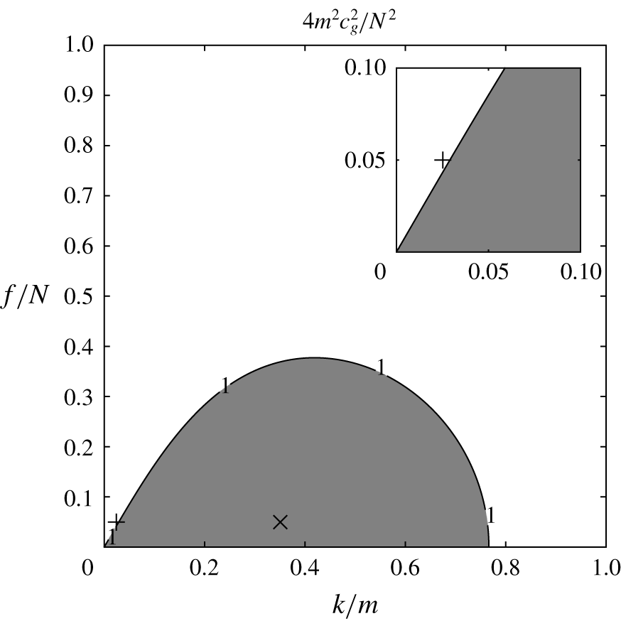
In the present paper we extend the study of Reference Thomas, Buhler and SmithTBS18 to mode-one waves in the three-dimensional rotating Boussinesq equations, which is the setting of Reference Wagner and YoungWY15, although unlike Reference Wagner and YoungWY15, we do not consider the effects of non-constant stratification. Our results differ significantly from those of Reference Wagner and YoungWY15 in two respects. First, we find that a co-moving barotropic Bretherton flow dominates the mean-flow response, whereas Reference Wagner and YoungWY15 assumed the barotropic mean-flow component to be negligible. Second, we reveal a new criterion in (3.10) that determines whether a co-moving baroclinic mean-flow solution exists or whether there is an unceasing radiation of waves. This is a new kind of result in the sense that that the transition from a co-moving to wave-radiating solution occurs at a critical combination of flow parameters (wave aspect ratio and the ratio of rotation to stratification frequencies – see figure 1), rather than as a result of changing the domain geometry from three- to two-dimensional. We investigate this situation in full detail by using asymptotic theory combined with direct numerical simulations of a Galerkin-truncated nonlinear hydrostatic Boussinesq model, which corroborates all aspects of our theory.
The outline of the paper is as follows: the governing equations and their asymptotic expansions are described in § 2, the modal solution of the equations to second order in wave amplitude is given in § 3 and numerical simulations are presented in § 4. Concluding comments are offered in § 5.
2 Governing equations
We consider the standard inviscid  $f$-plane Boussinesq equations
 $$\begin{eqnarray}\displaystyle & \displaystyle \boldsymbol{u}_{t}+\boldsymbol{u}\boldsymbol{\cdot }\unicode[STIX]{x1D735}\boldsymbol{u}+f\hat{\boldsymbol{z}}\times \boldsymbol{u}+\unicode[STIX]{x1D735}P-b\hat{\boldsymbol{z}}=0, & \displaystyle\end{eqnarray}$$
 $$\begin{eqnarray}\displaystyle & \displaystyle b_{t}+\boldsymbol{u}\boldsymbol{\cdot }\unicode[STIX]{x1D735}b+N^{2}w=0, & \displaystyle\end{eqnarray}$$
 $$\begin{eqnarray}\displaystyle & \displaystyle \unicode[STIX]{x1D735}\boldsymbol{\cdot }\boldsymbol{u}=0, & \displaystyle\end{eqnarray}$$
 $\boldsymbol{u}=(u,v,w)$ is the velocity,
 $\hat{\boldsymbol{z}}$ is the vertical unit vector and
 $b$ is the buoyancy. The Coriolis parameter
 $f$ and the buoyancy frequency
 $N$ are constant and we assume an ocean with constant depth
 $H$ and dynamically passive, rigid-lid boundary conditions
 $$\begin{eqnarray}w=0\quad \text{and}\quad b=0\quad \text{at}\quad z=0\quad \text{and}\quad z=-H.\end{eqnarray}$$
The materially conserved PV is
 $$\begin{eqnarray}q=fN^{2}+fb_{z}+N^{2}(v_{x}-u_{y})+(\unicode[STIX]{x1D735}\times \boldsymbol{u})\boldsymbol{\cdot }\unicode[STIX]{x1D735}b,\end{eqnarray}$$
and we consider it to be everywhere fixed to its undisturbed background value  $q=fN^{2}$; hence we have the global constraint
 $$\begin{eqnarray}v_{x}-u_{y}+\frac{f}{N^{2}}b_{z}+\frac{1}{N^{2}}(\unicode[STIX]{x1D735}\times \boldsymbol{u})\boldsymbol{\cdot }\unicode[STIX]{x1D735}b=0.\end{eqnarray}$$
As in Reference Thomas, Buhler and SmithTBS18, this relation constitutes our basic assumption of an entirely wave-induced flow.
2.1 Linear wavepacket solution
We assume the  $O(1)$ mean flow is zero and that the leading-order motion is linear waves, with non-dimensional small amplitude
 $a\ll 1$. The
 $O(a)$ wave velocity
 $\boldsymbol{u}^{\prime }=(u^{\prime },v^{\prime },w^{\prime })$, buoyancy
 $b^{\prime }$ and pressure
 $P^{\prime }$ satisfy the linearized Boussinesq equations
 $$\begin{eqnarray}\displaystyle & \displaystyle \boldsymbol{u}_{t}^{\prime }+f\hat{\boldsymbol{z}}\times \boldsymbol{u}^{\prime }+\unicode[STIX]{x1D735}P^{\prime }-b^{\prime }\hat{\boldsymbol{z}}=0, & \displaystyle\end{eqnarray}$$
 $$\begin{eqnarray}\displaystyle & \displaystyle b_{t}^{\prime }+N^{2}w^{\prime }=0, & \displaystyle\end{eqnarray}$$
 $$\begin{eqnarray}\displaystyle & \displaystyle \unicode[STIX]{x1D735}\boldsymbol{\cdot }\boldsymbol{u}^{\prime }=0. & \displaystyle\end{eqnarray}$$
 $v_{x}^{\prime }-u_{y}^{\prime }+fb_{z}^{\prime }/N^{2}=0$. We assume a wavepacket that is slowly varying in time and in the horizontal directions, but not in the vertical. We define
 $\unicode[STIX]{x1D707}\ll 1$ as the ratio of the primary wavelength to the horizontal wavepacket scale, the usual Wentzel–Kramers–Brillouin (WKB) parameter associated with wavepacket analysis. Because of the
 $f$-plane assumption, we can assume the wavepacket travels in the
 $x$-direction without loss of generality, so that only the
 $x$-component of the group velocity is non-zero. If we introduce the packet-centred slow variables
 $$\begin{eqnarray}X=\unicode[STIX]{x1D707}k(x-c_{g}t),\quad Y=\unicode[STIX]{x1D707}ky,\end{eqnarray}$$
then the leading-order linear fields can be written as (real parts understood)
 $$\begin{eqnarray}\displaystyle & \displaystyle u^{\prime }=\text{i}\frac{\unicode[STIX]{x1D714}}{k}aA(X,Y)\cos (mz)\text{e}^{\text{i}(kx-\unicode[STIX]{x1D714}t+\unicode[STIX]{x1D6FC})}, & \displaystyle\end{eqnarray}$$
 $$\begin{eqnarray}\displaystyle & \displaystyle v^{\prime }=\frac{f}{k}aA(X,Y)\cos (mz)\text{e}^{\text{i}(kx-\unicode[STIX]{x1D714}t+\unicode[STIX]{x1D6FC})}, & \displaystyle\end{eqnarray}$$
 $$\begin{eqnarray}\displaystyle & \displaystyle w^{\prime }=\frac{\unicode[STIX]{x1D714}}{m}aA(X,Y)\sin (mz)\text{e}^{\text{i}(kx-\unicode[STIX]{x1D714}t+\unicode[STIX]{x1D6FC})}, & \displaystyle\end{eqnarray}$$
 $$\begin{eqnarray}\displaystyle & \displaystyle b^{\prime }=-\text{i}\frac{N^{2}}{m}aA(X,Y)\sin (mz)\text{e}^{\text{i}(kx-\unicode[STIX]{x1D714}t+\unicode[STIX]{x1D6FC})}. & \displaystyle\end{eqnarray}$$
 $k$ is the horizontal wavenumber,
 $m$ is the modal vertical wavenumber (an integer multiple of
 $\unicode[STIX]{x03C0}/H$),
 $\unicode[STIX]{x1D6FC}$ is a phase shift to be used subsequently for averaging,
 $c_{g}=\unicode[STIX]{x2202}\unicode[STIX]{x1D714}/\unicode[STIX]{x2202}k$ is the horizontal group velocity in the
 $x$-direction and
 $$\begin{eqnarray}\unicode[STIX]{x1D714}=+\sqrt{\frac{N^{2}k^{2}+f^{2}m^{2}}{k^{2}+m^{2}}}\end{eqnarray}$$
is the positive frequency branch. Recall that we have assumed the wavenumber in the  $y$-direction is zero. The wavepacket envelope function is a Gaussian
 $$\begin{eqnarray}A(X,Y)=\text{e}^{-(X^{2}+Y^{2})/2}.\end{eqnarray}$$
2.2 Eulerian-mean equations
The Eulerian-mean flow is defined as the flow averaged over the wavepacket phase shift  $\unicode[STIX]{x1D6FC}\in [0,2\unicode[STIX]{x03C0})$, which leads to the usual Reynolds-averaged Boussinesq equations for the Eulerian-mean fields, i.e.
 $$\begin{eqnarray}\displaystyle & \displaystyle \overline{\boldsymbol{u}}_{t}+f\hat{\boldsymbol{z}}\times \overline{\boldsymbol{u}}+\unicode[STIX]{x1D735}\overline{P}-\overline{b}\hat{\boldsymbol{z}}=-\boldsymbol{F}, & \displaystyle\end{eqnarray}$$
 $$\begin{eqnarray}\displaystyle & \displaystyle \overline{b}_{t}+N^{2}\overline{w}=-F^{b}, & \displaystyle\end{eqnarray}$$
 $$\begin{eqnarray}\displaystyle & \displaystyle \unicode[STIX]{x1D735}\boldsymbol{\cdot }\overline{\boldsymbol{u}}=0. & \displaystyle\end{eqnarray}$$
 $\boldsymbol{F}=(F^{u},F^{v},F^{w})$ and
 $F^{b}$ are the Reynolds flux divergence terms
 $$\begin{eqnarray}\boldsymbol{F}=\unicode[STIX]{x2202}_{j}\overline{(\boldsymbol{u}^{\prime }u_{j}^{\prime })}\quad \text{and}\quad F^{b}=\unicode[STIX]{x2202}_{j}\overline{(b^{\prime }u_{j}^{\prime })},\end{eqnarray}$$
where the Einstein summation convention is used. The Eulerian-mean equations are exact, but we only seek to solve them asymptotically for a small-amplitude wavepacket. However, a straightforward progression to the next-order response runs into a problem.
First, note that since the wavepacket is slowly varying in the horizontal directions and time, derivatives with respect to  $x,y,t$ of averaged wave interaction quantities are
 $O(\unicode[STIX]{x1D707}a^{2})$, whereas derivatives with respect to
 $z$ of averaged wave interaction quantities are
 $O(a^{2})$, asymptotically much larger. We assume that the mean flow inherits these scaling properties.
Next, recall that our  $O(a)$ linear wavepacket solution is only accurate to leading order in the WKB parameter,
 $\unicode[STIX]{x1D707}$. In particular, it does not include corrections to the wave solution at
 $O(\unicode[STIX]{x1D707}a)$. But we are interested in the
 $O(a^{2})$ mean-flow response on the time scale
 $O(1/\unicode[STIX]{x1D707})$, which allows the wavepacket to travel a distance comparable to its own diameter. In general, over such a long time the time integral of an
 $O(\unicode[STIX]{x1D707}a^{2})$ forcing quantity could be as large as
 $O(a^{2})$, and we would therefore need to retain Reynolds terms accurate up to
 $O(\unicode[STIX]{x1D707}a^{2})$ in order to ensure asymptotic accuracy. This would be automatic if the wavepacket were slowly varying in all three spatial directions, but here the vertical derivatives of averaged fields are
 $O(1)$.
To make this explicit, equation (2.7) shows us that  $\overline{u^{\prime }w^{\prime }}\sim O(\unicode[STIX]{x1D707}a^{2})$ and
 $\overline{w^{\prime }b^{\prime }}=0$, thus the
 $O(a)$ linear wave field is sufficient to compute
 $F^{u},F^{b}$, accurate up to
 $O(\unicode[STIX]{x1D707}a^{2})$. However, in general,
 $\overline{(v^{\prime }w^{\prime })}_{z}$ in
 $F^{v}$ and
 $\overline{(w^{\prime 2})}_{z}$ in
 $F^{w}$ do not vanish. Thus, it seems that we would need
 $O(\unicode[STIX]{x1D707}a)$ wave fields in order to compute
 $F^{v}$ and
 $F^{w}$ accurate up to
 $O(\unicode[STIX]{x1D707}a^{2})$, which is a very big obstacle.
The above argument is based on a worst-case scenario, in which  $O(\unicode[STIX]{x1D707}a^{2})$ forcing terms create a resonantly growing mean-flow response that breaks the asymptotics. It is entirely possible that these forcing terms would only lead to non-resonant mean-flow responses that are uniformly bounded in time at
 $O(\unicode[STIX]{x1D707}a^{2})$, and therefore ignorable. However, arriving at such a conclusion with the Eulerian-mean equations is a challenging task.
We show below that, when the mean-flow response problem is recast for a Lagrangian mean, this asymptotic hurdle does not arise; this demonstrates a posteriori that the  $O(\unicode[STIX]{x1D707}a^{2})$ forcing terms must be associated with harmless Stokes corrections, which do not grow resonantly in time. This is a satisfying outcome.
2.3 Lagrangian-mean equations
Let  $\unicode[STIX]{x1D743}^{\prime }=(\unicode[STIX]{x1D709}^{\prime },\unicode[STIX]{x1D702}^{\prime },\unicode[STIX]{x1D701}^{\prime })$ be linear particle displacements defined by
 $$\begin{eqnarray}\unicode[STIX]{x2202}_{t}\unicode[STIX]{x1D743}^{\prime }=\boldsymbol{u}^{\prime }\end{eqnarray}$$
and  $\overline{\unicode[STIX]{x1D743}^{\prime }}=0$. For any field
 $\unicode[STIX]{x1D6F7}$ we define its Lagrangian mean
 $\overline{\unicode[STIX]{x1D6F7}}^{L}=\overline{\unicode[STIX]{x1D6F7}}^{S}+\overline{\unicode[STIX]{x1D6F7}}$, where
 $\overline{\unicode[STIX]{x1D6F7}}^{S}=\overline{\unicode[STIX]{x1D743}^{\prime }\boldsymbol{\cdot }\unicode[STIX]{x1D735}\unicode[STIX]{x1D6F7}^{\prime }}$ is the leading-order Stokes correction and
 $\overline{\unicode[STIX]{x1D6F7}}$ is the Eulerian mean of
 $\unicode[STIX]{x1D6F7}$ (as in, e.g. Bühler Reference Bühler2014). Adding
 $\overline{\boldsymbol{u}}_{t}^{S}+f\hat{\boldsymbol{z}}\times \overline{\boldsymbol{u}}^{S}-\overline{b}^{S}\hat{\boldsymbol{z}}$ to (2.10a) and using the linear equations we find
 $$\begin{eqnarray}\overline{\boldsymbol{u}}_{t}^{L}+f\hat{\boldsymbol{z}}\times \overline{\boldsymbol{u}}^{L}-\overline{b}^{L}\hat{\boldsymbol{z}}+\unicode[STIX]{x1D735}\overline{P}=-\overline{\unicode[STIX]{x1D735}P}^{S},\end{eqnarray}$$
where  $\overline{\unicode[STIX]{x1D735}P}^{S}$ is the Stokes correction to
 $\unicode[STIX]{x1D735}P$. Similarly, adding
 $\overline{b}_{t}^{S}+N^{2}\overline{w}^{S}$ to (2.10b) leads to
 $$\begin{eqnarray}\overline{b}_{t}^{L}+N^{2}\overline{w}^{L}=0.\end{eqnarray}$$
Characteristically for Lagrangian-mean equations of material invariants, this equation has no eddy forcing term (Andrews & McIntyre Reference Andrews and McIntyre1978). Finally, we add  $\unicode[STIX]{x1D735}\boldsymbol{\cdot }\overline{\boldsymbol{u}}^{S}$ to (2.10c) and get
 $$\begin{eqnarray}\unicode[STIX]{x1D735}\boldsymbol{\cdot }\overline{\boldsymbol{u}}^{L}={\textstyle \frac{1}{2}}\unicode[STIX]{x2202}_{t}\unicode[STIX]{x2202}_{i}\unicode[STIX]{x2202}_{j}\overline{(\unicode[STIX]{x1D709}_{i}^{\prime }\unicode[STIX]{x1D709}_{j}^{\prime })}\approx {\textstyle \frac{1}{2}}\unicode[STIX]{x2202}_{t}\overline{(\unicode[STIX]{x1D701}^{\prime 2})}_{zz}.\end{eqnarray}$$
This is the divergence effect for the Lagrangian-mean flow (Andrews & McIntyre Reference Andrews and McIntyre1978); the second form shows the dominant term in the present situation. Whilst  $\unicode[STIX]{x1D735}\boldsymbol{\cdot }\overline{\boldsymbol{u}}^{L}$ is non-zero, it is still determined directly by the linear wave solution. The boundary conditions for the Lagrangian-mean flow at
 $z=0$ and
 $z=-H$ are simply
 $\overline{w}^{L}=0$ and
 $\overline{b}^{L}=0$.
The only non-trivial step is the following manipulation of  $\overline{\unicode[STIX]{x1D735}P}^{S}$, which mimics a similar calculation in the shallow-water system studied by Reference Thomas, Buhler and SmithTBS18. We show in appendix A that the equality
 $$\begin{eqnarray}\overline{\unicode[STIX]{x1D735}P}^{S}={\textstyle \frac{1}{2}}\unicode[STIX]{x1D735}\overline{P}^{S}-\boldsymbol{p}_{t}-{\textstyle \frac{1}{4}}\unicode[STIX]{x1D735}\overline{(\unicode[STIX]{x1D743}^{\prime 2})}_{tt}\end{eqnarray}$$
holds, where  $\boldsymbol{p}=(p^{x},p^{y},p^{z})$ is the
 $O(a^{2})$ Lagrangian-mean pseudomomentum defined in Andrews & McIntyre (Reference Andrews and McIntyre1978) as
 $$\begin{eqnarray}p^{i}=-\overline{\unicode[STIX]{x1D709}_{j,i}^{\prime }(u_{j}^{\prime }+{\textstyle \frac{1}{2}}[f\hat{\boldsymbol{z}}\times \unicode[STIX]{x1D743}^{\prime }]_{j})}.\end{eqnarray}$$
The steady version of (2.16) was derived and used in Wagner & Young (Reference Wagner and Young2015). Equation (2.13) now becomes
 $$\begin{eqnarray}\overline{\boldsymbol{u}}_{t}^{L}+f\hat{\boldsymbol{z}}\times \overline{\boldsymbol{u}}^{L}+\unicode[STIX]{x1D735}B-\overline{b}^{L}\hat{\boldsymbol{z}}=\boldsymbol{p}_{t},\end{eqnarray}$$
where
 $$\begin{eqnarray}B=\overline{P}+{\textstyle \frac{1}{2}}\overline{P}^{S}-{\textstyle \frac{1}{4}}\unicode[STIX]{x2202}_{t}^{2}\overline{(\unicode[STIX]{x1D743}^{\prime 2})}.\end{eqnarray}$$
Thus  $B$ acts like a pressure term for the Lagrangian-mean equations. In principle,
 $B$ can be found from taking the divergence of (2.18) and using (2.15). In other words, (2.18), (2.15) and (2.14) together form a closed set of mean-flow equations with explicit
 $O(\unicode[STIX]{x1D707}a^{2})$ forcing terms that require nothing more than the leading-order linear fields. This confirms that the ‘missing’ forcing terms in the Eulerian-mean formulation are related to the Stokes corrections.
Before moving on, we note a consequence of the PV constraint (2.4). Adding  $f\overline{b}_{z}^{S}/N^{2}+\overline{v}_{x}^{S}-\overline{u}_{y}^{S}$ to the Eulerian mean of (2.4) eventually results in the Lagrangian-mean constraint
 $$\begin{eqnarray}\overline{v}_{x}^{L}-\overline{u}_{y}^{L}+\frac{f}{N^{2}}\overline{b}_{z}^{L}=\hat{\boldsymbol{z}}\boldsymbol{\cdot }(\unicode[STIX]{x1D735}\times \boldsymbol{p})-\frac{1}{2}f\unicode[STIX]{x2202}_{i}\unicode[STIX]{x2202}_{j}\overline{(\unicode[STIX]{x1D709}_{i}^{\prime }\unicode[STIX]{x1D709}_{j}^{\prime })}.\end{eqnarray}$$
This can also be derived using the exact formulae for the Lagrangian-mean PV  $\overline{q}^{L}$ (see Holmes-Cerfon et al. Reference Holmes-Cerfon, Bühler and Ferrari2011; Bühler Reference Bühler2014).
The mean-flow problem is simplified by noting that the mean flow is hydrostatic. This can be seen from (2.15), which implies  $\overline{w}^{L}=O(\unicode[STIX]{x1D707}a^{2})$, thus
 $\overline{w}_{t}^{L}=O(\unicode[STIX]{x1D707}^{2}a^{2})$ and we can neglect
 $\overline{w}_{t}^{L}$ in the vertical Lagrangian-mean momentum equation (the same is true for its Eulerian counterpart). We thus have
 $$\begin{eqnarray}\overline{b}^{L}=\unicode[STIX]{x2202}_{z}B-\unicode[STIX]{x2202}_{t}p^{z}=\unicode[STIX]{x2202}_{z}B+O(\unicode[STIX]{x1D707}^{2}a^{2}).\end{eqnarray}$$
The last step follows because the vertical pseudomomentum  $p^{z}=O(\unicode[STIX]{x1D707}a^{2})$ (which can be obtained by substituting (2.7) into (2.17)), and so its time derivative is
 $O(\unicode[STIX]{x1D707}^{2}a^{2})$. Hence, the leading-order diagnostic equation
 $\overline{b}^{L}=B_{z}$ allows us to eliminate
 $\overline{b}^{L}$ in favour of
 $B$ as needed. Specifically, combining (2.14) and (2.15) yields
 $$\begin{eqnarray}-\frac{1}{N^{2}}\unicode[STIX]{x2202}_{t}B_{zz}+(\overline{u}_{x}^{L}+\overline{v}_{y}^{L})=\frac{1}{2}\unicode[STIX]{x2202}_{t}\overline{(\unicode[STIX]{x1D701}^{\prime 2})}_{zz},\end{eqnarray}$$
where several  $O(\unicode[STIX]{x1D707}^{2}a^{2})$ terms have been neglected. The horizontal components of (2.18) and (2.22) now form a closed set for
 $\{\overline{u}^{L},\overline{v}^{L},B\}$, which does not include
 $\overline{w}^{L}$ and
 $\overline{b}^{L}$ explicitly anymore.
3 Modal solution for the mean-flow response
We now proceed to solve the mean-flow equations by first expanding into vertical modes. The forcing terms are quadratic combinations of the linear wave fields, all of which feature the same vertical wavenumber  $m$. Hence, the leading-order mean-flow response consists of a barotropic mode with zero vertical wavenumber and a baroclinic mode with vertical wavenumber
 $2m$.
3.1 Barotropic mode
The barotropic mode of any field is denoted by a subscript zero and equals the depth average of that field, e.g.
 $$\begin{eqnarray}(\overline{u}_{0}^{L},\overline{v}_{0}^{L})=\frac{1}{H}\int _{-H}^{0}(\overline{u}^{L},\overline{v}^{L})\,\text{d}z.\end{eqnarray}$$
The boundary conditions imply  $\overline{b}_{0}^{L}=0$. From (2.22), the barotropic velocity field is horizontally non-divergent, thus we define
 $\unicode[STIX]{x1D713}_{0}$ as the barotropic streamfunction, such that
 $\overline{u}_{0}^{L}=-\unicode[STIX]{x2202}_{y}\unicode[STIX]{x1D713}_{0}$,
 $\overline{v}_{0}^{L}=\unicode[STIX]{x2202}_{x}\unicode[STIX]{x1D713}_{0}$. By taking the vertical component of the curl of (2.18) and depth integrating, we obtain
 $$\begin{eqnarray}\unicode[STIX]{x1D6FB}_{h}^{2}\unicode[STIX]{x1D713}_{0}=\unicode[STIX]{x2202}_{x}\,p_{0}^{y}-\unicode[STIX]{x2202}_{y}\,p_{0}^{x},\quad \text{where }\unicode[STIX]{x1D735}_{h}=(\unicode[STIX]{x2202}_{x},\unicode[STIX]{x2202}_{y}).\end{eqnarray}$$
This is the two-dimensional version of the classic Bretherton return flow around a wavepacket found by Reference BrethertonB69, which is a non-divergent dipolar return flow attached to the wavepacket. Another interpretation of (3.2) is that  $(\overline{u}_{0}^{L},\overline{v}_{0}^{L})$ is the least-squares projection of
 $(p_{0}^{x},p_{0}^{y})$ onto non-divergent vector fields (Bühler Reference Bühler2014). Notably,
 $\unicode[STIX]{x1D713}_{0}\sim O(\unicode[STIX]{x1D707}^{-1}a^{2})$ and the barotropic velocity is
 $O(a^{2})$, so of the same strength as the barotropic pseudomomentum. Also, equation (3.2) is a diagnostic relation and since pseudomomentum is steady in the frame moving with the group velocity, the Bretherton flow is also steady in that frame.
3.2 Baroclinic mode
For the baroclinic component of the mean-flow response we use tildes to denote the respective coefficient functions that depend on  $(x,y,t)$. In particular, the baroclinic component of
 $(\overline{u}^{L},\overline{v}^{L})$ is
 $(\widetilde{u},\widetilde{v})\cos (2mz)$, that of
 $\overline{b}^{L}$ is
 $\widetilde{b}\sin (2mz)$ and that of
 $B$ is
 $\widetilde{B}\cos (2mz)$. For the forcing terms, the baroclinic part of the horizontal
 $\boldsymbol{p}$ is
 $\widetilde{\boldsymbol{p}}\cos (2mz)$, and we use the shorthand
 $G(x,y)\cos (2mz)$ for the baroclinic part of
 $N^{2}/(8m^{2})\overline{(\unicode[STIX]{x1D701}^{\prime 2})}_{zz}$. By projecting (2.18) and (2.22) we then obtain
 $$\begin{eqnarray}\displaystyle & \widetilde{u}_{t}-f\hspace{1.0pt}\widetilde{v}+\widetilde{B}_{x}=\widetilde{p^{x}}_{t}, & \displaystyle\end{eqnarray}$$
 $$\begin{eqnarray}\displaystyle & \widetilde{v}_{t}+f\hspace{1.25pt}\widetilde{u}+\widetilde{B}_{y}=\widetilde{p^{y}}_{t}, & \displaystyle\end{eqnarray}$$
 $$\begin{eqnarray}\displaystyle & \widetilde{B}_{t}+\frac{N^{2}}{4m^{2}}(\widetilde{u}_{x}+\widetilde{v}_{y})=G_{t}, & \displaystyle\end{eqnarray}$$
 $$\begin{eqnarray}\widetilde{b}=-2m\widetilde{B}.\end{eqnarray}$$
These are forced shallow-water equations. For convenience, we define the following two operators:
 $$\begin{eqnarray}{\mathcal{L}}_{1}=\unicode[STIX]{x2202}_{t}^{2}+f^{2}-\frac{N^{2}}{4m^{2}}\unicode[STIX]{x1D6FB}_{h}^{2}\quad \text{and}\quad {\mathcal{L}}_{2}=f^{2}-\left(\frac{N^{2}}{4m^{2}}-c_{g}^{2}\right)\unicode[STIX]{x2202}_{x}^{2}-\frac{N^{2}}{4m^{2}}\unicode[STIX]{x2202}_{y}^{2},\end{eqnarray}$$
where  ${\mathcal{L}}_{1}$ will be shown to become
 ${\mathcal{L}}_{2}$ in the co-moving frame. From (3.3) and (3.4), the decoupled equations for the flow divergence, curl and buoyancy can be derived:
 $$\begin{eqnarray}\displaystyle & \displaystyle {\mathcal{L}}_{1}[\unicode[STIX]{x1D735}_{h}\boldsymbol{\cdot }\widetilde{\boldsymbol{u}}]=\unicode[STIX]{x2202}_{t}[\unicode[STIX]{x2202}_{t}\unicode[STIX]{x1D735}_{h}\boldsymbol{\cdot }\widetilde{\boldsymbol{p}}+f\hat{\boldsymbol{z}}\boldsymbol{\cdot }(\unicode[STIX]{x1D735}_{h}\times \widetilde{\boldsymbol{p}})-\unicode[STIX]{x1D735}_{h}^{2}G], & \displaystyle\end{eqnarray}$$
 $$\begin{eqnarray}\displaystyle & \displaystyle {\mathcal{L}}_{1}[\hat{\boldsymbol{z}}\boldsymbol{\cdot }(\unicode[STIX]{x1D735}_{h}\times \widetilde{\boldsymbol{u}})]=\left(\unicode[STIX]{x2202}_{t}^{2}-\frac{N^{2}}{4m^{2}}\unicode[STIX]{x1D6FB}_{h}^{2}\right)\hat{\boldsymbol{z}}\boldsymbol{\cdot }(\unicode[STIX]{x1D735}_{h}\times \widetilde{\boldsymbol{p}})-f\unicode[STIX]{x2202}_{t}\unicode[STIX]{x1D735}_{h}\boldsymbol{\cdot }\widetilde{\boldsymbol{p}}+f\unicode[STIX]{x1D6FB}_{h}^{2}G, & \displaystyle\end{eqnarray}$$
 $$\begin{eqnarray}\displaystyle & \displaystyle {\mathcal{L}}_{1}\left[\frac{2m}{N^{2}}\widetilde{b}+\frac{4m^{2}}{N^{2}}G\right]=\unicode[STIX]{x2202}_{t}\unicode[STIX]{x1D735}_{h}\boldsymbol{\cdot }\widetilde{\boldsymbol{p}}+f\hat{\boldsymbol{z}}\boldsymbol{\cdot }(\unicode[STIX]{x1D735}_{h}\times \widetilde{\boldsymbol{p}})-\unicode[STIX]{x1D6FB}_{h}^{2}G. & \displaystyle\end{eqnarray}$$
 $$\begin{eqnarray}(\widetilde{u},\widetilde{v})=\unicode[STIX]{x1D735}_{h}\unicode[STIX]{x1D719}_{2}+\hat{\boldsymbol{z}}\times \unicode[STIX]{x1D735}_{h}\unicode[STIX]{x1D713}_{2},\quad (\widetilde{p}^{x},\widetilde{p}^{y})=\unicode[STIX]{x1D735}_{h}\unicode[STIX]{x1D719}^{\boldsymbol{p}}+\hat{\boldsymbol{z}}\times \unicode[STIX]{x1D735}_{h}\unicode[STIX]{x1D713}^{\boldsymbol{p}},\end{eqnarray}$$
together with suitable decay conditions for the potentials at infinity. This results in
 $$\begin{eqnarray}\displaystyle & \displaystyle {\mathcal{L}}_{1}\unicode[STIX]{x1D719}_{2}=\unicode[STIX]{x2202}_{t}(\unicode[STIX]{x2202}_{t}\unicode[STIX]{x1D719}^{\boldsymbol{p}}+f\unicode[STIX]{x1D713}^{\boldsymbol{p}}-G), & \displaystyle\end{eqnarray}$$
 $$\begin{eqnarray}\displaystyle & \displaystyle {\mathcal{L}}_{1}\unicode[STIX]{x1D713}_{2}=\left(\unicode[STIX]{x2202}_{t}^{2}-\frac{N^{2}}{4m^{2}}\unicode[STIX]{x1D6FB}_{h}^{2}\right)\unicode[STIX]{x1D713}^{\boldsymbol{p}}-f\unicode[STIX]{x2202}_{t}\unicode[STIX]{x1D719}^{\boldsymbol{p}}+fG, & \displaystyle\end{eqnarray}$$
 $$\begin{eqnarray}\displaystyle & \displaystyle {\mathcal{L}}_{1}\left[\frac{2m}{N^{2}}\widetilde{b}+\frac{4m^{2}}{N^{2}}G\right]=\unicode[STIX]{x2202}_{t}\unicode[STIX]{x1D6FB}_{h}^{2}\unicode[STIX]{x1D719}^{\boldsymbol{p}}+f\unicode[STIX]{x1D6FB}_{h}^{2}\unicode[STIX]{x1D713}^{\boldsymbol{p}}. & \displaystyle\end{eqnarray}$$
3.3 Co-moving and resonant solutions
Co-moving solutions to the mean-flow equations decay at infinity and are steady in the frame moving with the wavepacket, i.e. co-moving solution are functions of  $(x-c_{g}t,y)$ only. The barotropic Bretherton flow (3.2) is obviously always such a co-moving solution, and we now investigate under what conditions, if any, the baroclinic mean flow is as well. We do this by assuming a co-moving solution exists and then seek to find it. Hence, if we introduce the co-moving coordinate
 $x^{\prime }=x-c_{g}t$, replace
 $\unicode[STIX]{x2202}_{x}$ by
 $\unicode[STIX]{x2202}_{x}^{\prime }$,
 $\unicode[STIX]{x2202}_{t}$ by
 $-c_{g}\unicode[STIX]{x2202}_{x^{\prime }}$ in (3.8a)–(3.8c) and drop the primes, we obtain the steady set
 $$\begin{eqnarray}\displaystyle & \displaystyle {\mathcal{L}}_{2}\unicode[STIX]{x1D719}_{2}=-c_{g}\unicode[STIX]{x2202}_{x}(-c_{g}\unicode[STIX]{x2202}_{x}\unicode[STIX]{x1D719}^{\boldsymbol{p}}+f\unicode[STIX]{x1D713}^{\boldsymbol{p}}-G), & \displaystyle\end{eqnarray}$$
 $$\begin{eqnarray}\displaystyle & \displaystyle {\mathcal{L}}_{2}\unicode[STIX]{x1D713}_{2}=\left[\left(c_{g}^{2}-\frac{N^{2}}{4m^{2}}\right)\unicode[STIX]{x2202}_{x}^{2}-\frac{N^{2}}{4m^{2}}\unicode[STIX]{x2202}_{y}^{2}\right]\unicode[STIX]{x1D713}^{\boldsymbol{p}}+fc_{g}\unicode[STIX]{x2202}_{x}\unicode[STIX]{x1D719}^{\boldsymbol{p}}+fG, & \displaystyle\end{eqnarray}$$
 $$\begin{eqnarray}\displaystyle & \displaystyle {\mathcal{L}}_{2}\left[\frac{2m}{N^{2}}\widetilde{b}+\frac{4m^{2}}{N^{2}}G\right]=\unicode[STIX]{x1D6FB}_{h}^{2}(-c_{g}\unicode[STIX]{x2202}_{x}\unicode[STIX]{x1D719}^{\boldsymbol{p}}+f\unicode[STIX]{x1D713}^{\boldsymbol{p}}-G). & \displaystyle\end{eqnarray}$$
 ${\mathcal{L}}_{2}$. By inspection of (3.5), for
 $f\neq 0$,
 ${\mathcal{L}}_{2}$ is a modified Helmholtz operator, which guarantees decay at infinity only if the coefficients of the spatial derivatives have the same sign, i.e. only if
 $$\begin{eqnarray}\frac{N^{2}}{4m^{2}}>c_{g}^{2}.\end{eqnarray}$$
For  $f\neq 0$, the marginal case with an equal sign is also permitted, but not so for
 $f=0$. Hence, we have found in (3.10) a non-trivial criterion for the existence of a co-moving baroclinic response to the wavepacket: depending on the parameters, a wavepacket may or may not lead to a co-moving mean-flow solution. By contrast, in the analogous shallow-water analysis in Reference Thomas, Buhler and SmithTBS18, co-moving solutions always existed provided
 $f\neq 0$, which is a very different outcome. This contrasts again with non-rotating two-dimensional flows in the
 $x{-}z$ plane, for which Reference BrethertonB69, McIntyre (Reference McIntyre1973) and Van den Bremer et al. (Reference Van den Bremer, Yassin and Sutherland2019) found that a co-moving solution is possible only if
 $N^{2}/(4m^{2})=c_{g}^{2}$, a condition that is almost never satisfied.
If (3.10) is not satisfied, then the time-dependent solution includes resonantly forced mean-flow gravity waves, which are continuously shed from the wavepacket. This will be confirmed by the direct numerical simulations below. Further theoretical details on these resonant waves and the physical interpretation of the criterion (3.10) are given in appendix B.
In figure 1 we provide a regime diagram to illustrate that (3.10) is quite relevant for the physical inertia–gravity wave field in the ocean. The diagram shows the non-dimensional parameter  $4m^{2}c_{g}^{2}/N^{2}$, which by virtue of the dispersion relation is a function of
 $k/m$ and
 $f/N$ only. The second panel is a blow-up of the first near the origin, which is the region of most oceanic relevance where both
 $k/m$ and
 $f/N$ are small. If the rotation is strong enough (e.g.
 $f/N>0.4$) then co-moving solutions prevail for all wavepackets, but this is unrealistic for the ocean, where rotation is typically much weaker than that. Similarly, large enough
 $k/m$ rules out resonance, but oceanic waves tend to have low values of
 $k/m$, indeed, they are often modelled as hydrostatic waves for this reason. This makes apparent that resonant and co-moving solutions are both relevant for oceanic conditions. The
 $+$ and
 $\times$ symbols mark the parameters used in our numerical simulations, described in § 4. We will find that the parameters marked by
 $\times$ indeed corresponds to a resonant solution, and the those for
 $+$ to a co-moving solution.
Contour plot of  $4m^{2}c_{g}^{2}/N^{2}=4(k/m)^{2}[1-(f/N)^{2}]^{2}/\!\{[(k/m)^{2}+(f/N)^{2}][(k/m)^{2}+1]^{3}\!\}$ as a function of
 $k/m$ and
 $f/N$. Resonant solutions lie in the grey region, and co-moving solutions lie in the white region. The inset shows a close-up of the oceanically relevant region of parameter space. The
 $+$ and
 $\times$ symbols mark parameter values used in the simulations described in § 4.

3.4 Comparison with § 5.2 of Wagner & Young (Reference Wagner and Young2015)
Our mean-flow analysis differs in two places from that presented in § 5.2 of WY15 for the same wavepacket problem and constant  $N$. First, these authors employed a mean-flow time scale separation based on a low Rossby number assumption, which, as those authors point out, does not fully allow for propagating wavepackets as forcing terms. This suggests that their analysis might be most accurate for fairly slow wavepackets. Indeed, in terms of our analysis, their scaling amounts to neglecting the time derivatives in the baroclinic equations (3.8). This would imply
 $\unicode[STIX]{x1D719}_{2}=0$, and therefore a horizontally non-divergent Lagrangian-mean flow, and also the existence of a co-moving mean-flow solution for all wavepacket parameters, contrary to our findings. Presumably, in terms of our criterion (3.10), a very slow wavepacket simply corresponds to
 $c_{g}\rightarrow 0$, which then always satisfies the criterion. Thus, their more restrictive time scale assumption effectively filters the possibility of resonant mean-flow forcing.
Second, in keeping with their time scale assumption they derive a general equation for the three-dimensional Lagrangian-mean streamfunction  $\unicode[STIX]{x1D713}^{L}$ (their (5.1)),
 $$\begin{eqnarray}\left(\unicode[STIX]{x1D6FB}_{h}^{2}+\frac{f^{2}}{N^{2}}\unicode[STIX]{x2202}_{z}^{2}\right)\unicode[STIX]{x1D713}^{L}=\hat{\boldsymbol{z}}\boldsymbol{\cdot }\unicode[STIX]{x1D735}\times \boldsymbol{p}-\frac{f}{2}(\overline{\unicode[STIX]{x1D709}_{i}^{\prime }\unicode[STIX]{x1D709}_{j}^{\prime }})_{,ij}.\end{eqnarray}$$
This is consistent with the present PV constraint (2.20) applied to a quasi-geostrophic mean flow. They then note that, for a wavepacket with vertical modal wavenumber  $m$, the right-hand side is dominated by the term
 $-(f/2)\overline{(\unicode[STIX]{x1D701}^{\prime 2})}_{zz}$, so they neglect the pseudomomentum term and arrive at
 $$\begin{eqnarray}\left(\unicode[STIX]{x1D6FB}_{h}^{2}+\unicode[STIX]{x2202}_{z}\frac{f^{2}}{N^{2}}\unicode[STIX]{x2202}_{z}\right)\unicode[STIX]{x1D713}^{L}=-\frac{f}{2}\overline{(\unicode[STIX]{x1D701}^{\prime 2})}_{zz}.\end{eqnarray}$$
Notably, the source term now has no barotropic component whereas the pseudomomentum term had a barotropic component. Hence, the step from (3.11) to (3.12) loses the barotropic mean-flow response described in our (3.2), i.e. it loses the Bretherton flow. The reason for this loss is that, whilst the right-hand side of (3.11) is indeed dominated by the final term, the operator on the left-hand side is much more compliant for barotropic solutions, as it then loses the strong vertical derivatives term inside itself. This is what was described in § 3.1 in connection with the barotropic Bretherton flow. We write their baroclinic response (solution to equation (3.12)) as  $\unicode[STIX]{x1D713}^{L}=\unicode[STIX]{x1D713}_{WY}\cos (2mz)$ for comparison with our results.
In summary, our results differ from the calculation of Reference Wagner and YoungWY15 (for constant  $N$, in their § 5.2) by allowing for the possibility of a resonantly forced baroclinic mean-flow response, and by the demonstration of a strong,
 $O(a^{2})$ barotropic Bretherton flow for all wavepacket parameters.
4 Numerical simulations
4.1 The numerical model
In order to efficiently capture the three-dimensional dynamics of the wavepacket, we developed a Galerkin-truncated model of the hydrostatic Boussinesq equations that retains only the barotropic and first two baroclinic modes. The model equations are presented in appendix C. The truncated model conserves the energy,  $\frac{1}{2}\int (|\boldsymbol{u}|^{2}+b^{2}/N^{2})$, but does not materially conserve the exact nonlinear PV, as one would expect.
The boundary conditions are doubly periodic and the governing equations are solved using a fully dealiased pseudo-spectral method. An eighth-order hyper-diffusion is added to suppress numerical instability, and the hyper-viscosity  $\unicode[STIX]{x1D708}=\frac{1}{2}\unicode[STIX]{x0394}x/(\unicode[STIX]{x0394}tk_{max}^{8})$, where
 $k_{max}$ is the largest resolved horizontal wavenumber,
 $\unicode[STIX]{x0394}x$ is the grid spacing and
 $\unicode[STIX]{x0394}t$ is the time step. The number of grid points is
 $2048\times 2048$. The time step is determined by a Courant–Friedrichs–Lewy (CFL) condition based on the maximum of the initial velocity and phase speed of the primary wave, with the CFL number being
 $0.05$.
We consider two simulations, each initialized with a wavepacket in the gravest vertical mode with vertical wavenumber  $m=\unicode[STIX]{x03C0}/H$ (where
 $H$ is the height of the three-dimensional domain), located at
 $(x,y)=(0,0)$ in a laterally square domain of side length
 $L=16\unicode[STIX]{x03C0}/\unicode[STIX]{x1D707}k$. In each simulation, the stratification-to-rotation ratio
 $N/f$ is set to
 $20$, and the non-dimensional wave parameters are
 $a=0.01$ and
 $\unicode[STIX]{x1D707}=0.05$. These choices should allow sufficient scale separation between the domain and the wavepacket footprint to prevent the packet from ‘feeling itself’, thus approximating the infinite domain setting in which the analytical solutions are derived. The first simulation is set in a co-moving regime with wave aspect ratio
 $k/m=f/(2N)$, and the second is in a resonant regime with
 $k/m=7f/N$. The two simulations are denoted by the
 $+$ and
 $x$ in figure 1, respectively. In both cases, the phase speed is larger than the maximum initial velocity.
Note that, in practice, we set  $N=1$ and
 $k=1$ in the model equations of appendix C, and so effectively non-dimensionalize all the results by the horizontal length scale
 $1/k$ and time scale
 $1/N$. The height
 $H$ and effective
 $m$ are determined by the scaling choices for the simulations listed above.
4.2 The co-moving solution
In this section, we compare the numerical solution in the co-moving regime with our theoretical predictions. The philosophy behind the method of comparison is to initialize the numerical simulation with a superposition of the  $O(a)$ wavepacket and the
 $O(a^{2})$ analytically predicted Eulerian-mean-flow fields; if the analytical solution is correct, the Lagrangian-mean-flow fields should translate, without change, at the group velocity. Recall that the wavepacket sits in mode
 $m$, while the mean-flow response is entirely in modes
 $0$ (barotropic) and
 $2m$ (baroclinic), thus it suffices here to observe only these modes.
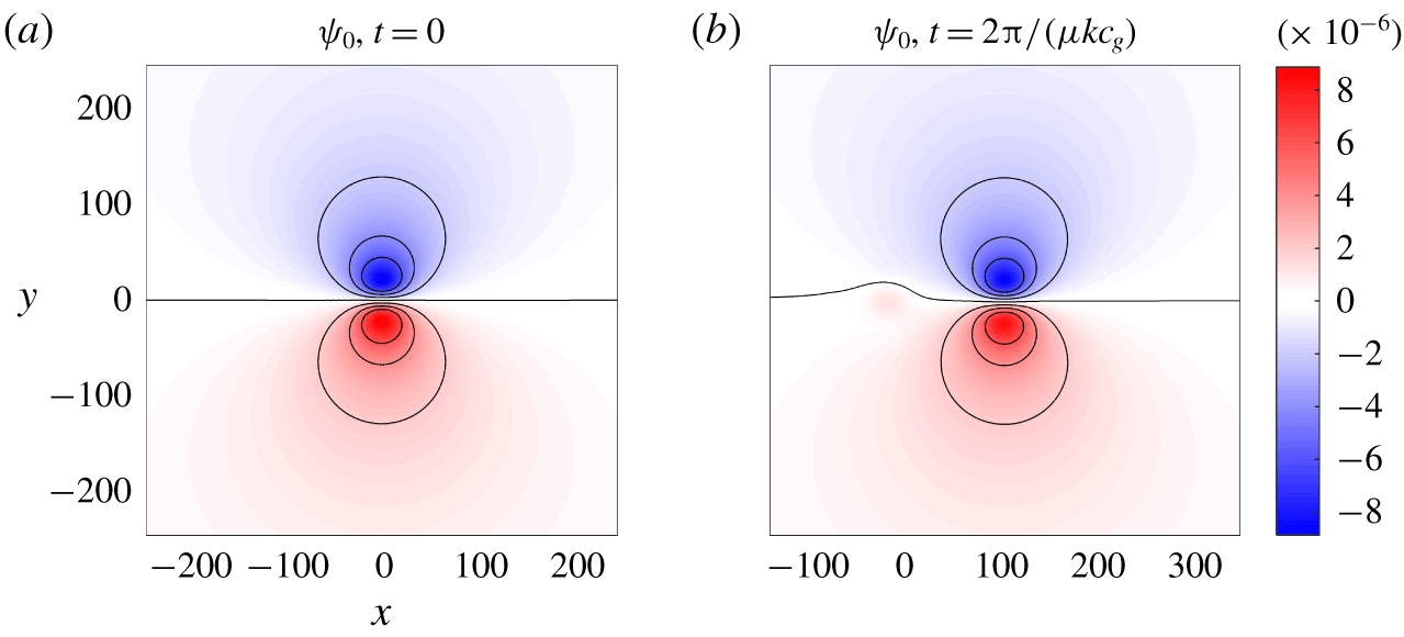
The numerically simulated Lagrangian-mean barotropic streamfunction for the co-moving case at (a)  $t=0$ and (b)
 $t=2\unicode[STIX]{x03C0}/(\unicode[STIX]{x1D707}kc_{g})\approx 11\,240$. Black lines are evenly spaced contours. The initial numerical field is the initial theoretical field, and at
 $t=2\unicode[STIX]{x03C0}/(\unicode[STIX]{x1D707}kc_{g})$ the theoretical field is a translation of the initial field along the
 $x$ direction for
 $2\unicode[STIX]{x03C0}/(\unicode[STIX]{x1D707}k)$.

In order to obtain the analytical solution at the initial time, we must solve (3.9), which itself requires the computation of wave quantities like the pseudomomentum and the wave vorticity (which is used in  $G$, defined above (3.3)). Moreover, to view the numerical solutions in the Lagrangian-mean frame at later times requires the computation of the Stokes correction at each time, which itself requires the current linear particle displacements. These can be computed from a single snapshot of the velocity and buoyancy fields using a ‘now-casting’ method described in appendix D. Together with averaging over the wavepacket phase shift
 $\unicode[STIX]{x1D6FC}$, this allows the computation of leading-order Stokes corrections directly, without any assumptions about slowly varying waves.
Figure 2 shows that the numerically simulated Lagrangian-mean barotropic streamfunction  $\unicode[STIX]{x1D713}_{0}$ translates in space, without any significant change, at a speed
 $c_{g}$, confirming that the numerical barotropic streamfunction remains essentially identical to its theoretical prediction. This flow is the Bretherton flow of Reference BrethertonB69. Note that this barotropic response appears in neither McIntyre (Reference McIntyre1973) nor Van den Bremer et al. (Reference Van den Bremer, Yassin and Sutherland2019), because each considered a two-dimensional setting.
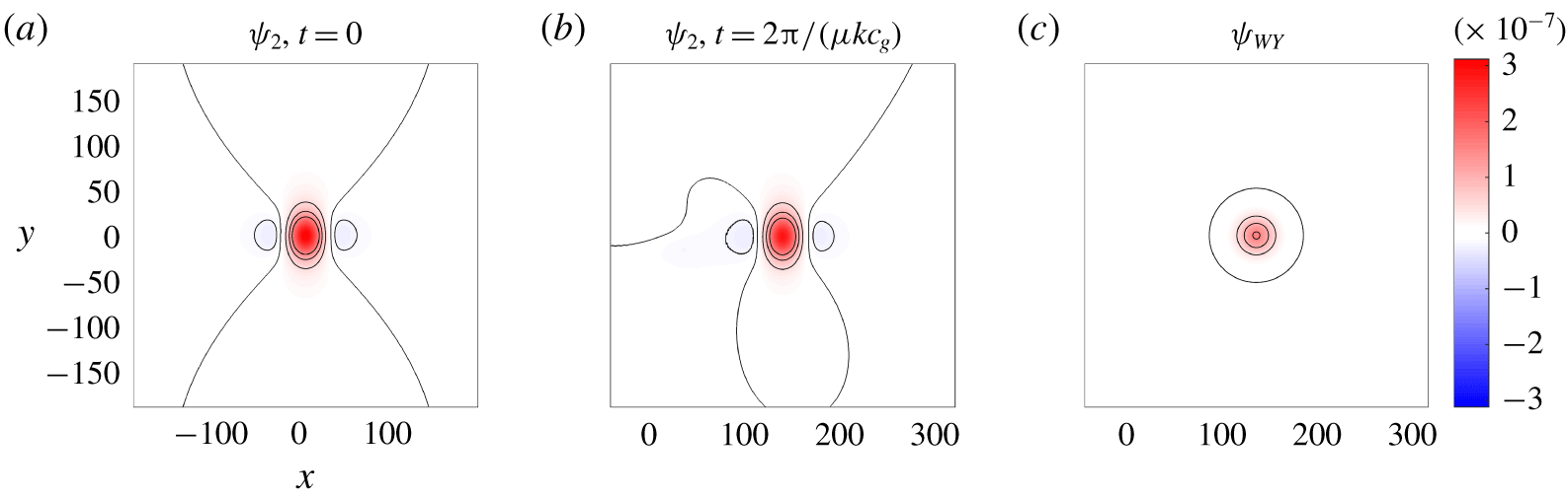
Figures 3(a) and 3(b) show that the Lagrangian-mean baroclinic streamfunction  $\unicode[STIX]{x1D713}_{2}$ is also a co-moving solution, translating at the group velocity, confirming that the theoretical prediction for the baroclinic response is also accurate. Note that some small-amplitude flow is induced at the initial location of the wavepacket because the initial PV is not exactly
 $fN^{2}$.
Figure 3(c) shows the Reference Wagner and YoungWY15 solution  $\unicode[STIX]{x1D713}_{WY}$ defined in § 3.4. Compared to the numerical solution,
 $\unicode[STIX]{x1D713}_{WY}$ does not capture the asymmetric shape of
 $\unicode[STIX]{x1D713}_{2}$, and underestimates its magnitude, due to the neglect of time-derivative terms.
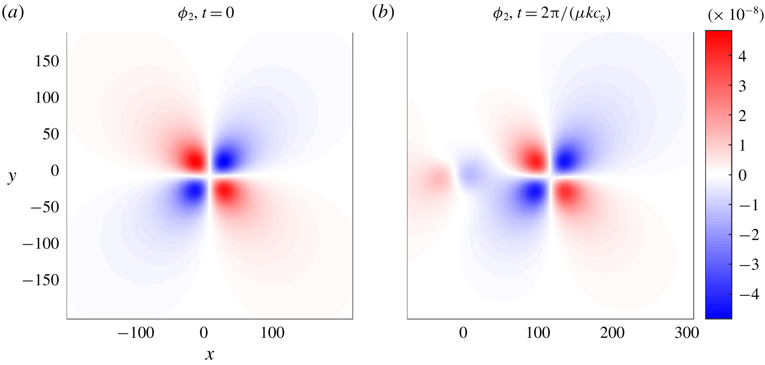
Figure 4 shows the numerical Lagrangian-mean baroclinic potential  $\unicode[STIX]{x1D719}_{2}$ (note that neglecting time derivatives in (3.8a) predicts
 $\unicode[STIX]{x1D719}_{2}=0$, which is clearly inaccurate). At
 $t=2\unicode[STIX]{x03C0}/(\unicode[STIX]{x1D707}kc_{g})$,
 $\unicode[STIX]{x1D719}_{2}$ is almost identical to its initial value (except for a small residual flow excited at the initial location of the wavepacket), again supporting the theoretical solution. Comparing the magnitudes of
 $\unicode[STIX]{x1D713}_{2}$,
 $\unicode[STIX]{x1D719}_{2}$ and
 $\unicode[STIX]{x1D713}_{0}$, we find that the Lagrangian-mean motion is dominated by the barotropic mode, which is missed by Reference Wagner and YoungWY15.
The numerically simulated Lagrangian-mean baroclinic streamfunction for the co-moving case at (a)  $t=0$ and (b)
 $t=2\unicode[STIX]{x03C0}/(\unicode[STIX]{x1D707}kc_{g})$. Panel (c) shows
 $\unicode[STIX]{x1D713}_{WY}$ at
 $t=2\unicode[STIX]{x03C0}/(\unicode[STIX]{x1D707}kc_{g})$. Black lines are contours corresponding to values
 $-0.2$, 0, 0.5, 1,
 $1.5\times 10^{-7}$. The initial numerical field is the initial theoretical field, and at
 $t=2\unicode[STIX]{x03C0}/(\unicode[STIX]{x1D707}kc_{g})$ the theoretical field is a translation of the initial field at
 $x=2\unicode[STIX]{x03C0}/(\unicode[STIX]{x1D707}k)$.

The numerically simulated Lagrangian-mean baroclinic potential for the co-moving case at (a)  $t=0$ and (b)
 $t=2\unicode[STIX]{x03C0}/(\unicode[STIX]{x1D707}kc_{g})$. The initial numerical field is the initial theoretical field, and at
 $t=2\unicode[STIX]{x03C0}/(\unicode[STIX]{x1D707}kc_{g})$ the theoretical field is a translation of the initial field at
 $x=2\unicode[STIX]{x03C0}/(\unicode[STIX]{x1D707}k)$.

4.2.1 Streamfunction and potential induced by non-hydrostatic wavepackets
In the above section, we demonstrated that the barotropic Lagrangian flow is much larger than the baroclinic Lagrangian flow. However, this is not expected to be the case when the primary wavepacket is non-hydrostatic. To see this, consider the limit of a baroclinic streamfunction and potential in the limit  $k/m\rightarrow \infty$ with fixed
 $f/N$. In this case,
 $c_{g}m/N\rightarrow 0$ and
 $fm/Nk\rightarrow 0$. Equation (3.9a) becomes
 $\unicode[STIX]{x1D6FB}_{h}^{2}\unicode[STIX]{x1D719}_{2}=0$, and (3.9b) becomes
 $\unicode[STIX]{x1D6FB}_{h}^{2}\unicode[STIX]{x1D713}_{2}=\unicode[STIX]{x2202}_{x}\,\widetilde{p}^{y}-\unicode[STIX]{x2202}_{y}\,\tilde{p}^{x}$.
To complete the argument, we compute the leading-order pseudomomentum by substituting (2.7) into the pseudomomentum definition (2.17), which (ignoring spatial derivatives of  $A$) gives
 $p^{y}=0$ and
 $$\begin{eqnarray}p^{x}=\frac{A^{2}a^{2}\unicode[STIX]{x1D714}}{4k}\left(\frac{k^{2}+m^{2}}{m^{2}}-\frac{k^{2}-m^{2}}{m^{2}}\cos 2mz\right)\xrightarrow[{\mathit{hydrostatic}}]{}\frac{A^{2}a^{2}\unicode[STIX]{x1D714}}{4k}(1+\cos 2mz).\end{eqnarray}$$
Thus, to  $O(a^{2})$ in the hydrostatic limit,
 $\tilde{p}^{x}=-p_{0}^{x}$, and so
 $\unicode[STIX]{x1D713}_{2}=-\unicode[STIX]{x1D713}_{0}$. Therefore, the magnitude of the baroclinic mode is the same as that of the barotropic mode. Notably, the net Lagrangian velocity at the surface and the bottom of the domain is zero, whereas it is generally non-zero in between.
4.3 The resonant solution
As shown in § 3.1, the barotropic mode is always a co-moving solution, thus we need only examine the evolution of the baroclinic mode. The initial condition consists of three parts: mode-one wavepacket, the analytically predicted co-moving barotropic Eulerian-mean flow and a baroclinic buoyancy  $N^{2}/(4m)a^{2}[A(\unicode[STIX]{x1D707}kx,\unicode[STIX]{x1D707}ky)]^{2}\cos (2mz)$. The baroclinic buoyancy is chosen to make the
 $O(a^{2})$ projection of the exact nonlinear PV onto mode
 $2m$ vanish, which approximates our uniform PV setting. As mentioned before, the exact PV in the Boussinesq system is not materially conserved in the truncated model, so initializing with exact uniform PV is not necessary (which is good because that turns out to be challenging). The current choice of initializing the mode
 $2m$ baroclinic field is the easiest way to ensure uniform baroclinic PV up to
 $O(a^{2})$. We first show the numerical results and then compare them with theory. To simplify the notation, we use
 $\overline{\boldsymbol{u}}_{2}^{L}$ to denote the Lagrangian mean of the baroclinic velocity amplitude
 $\tilde{\boldsymbol{u}}$.
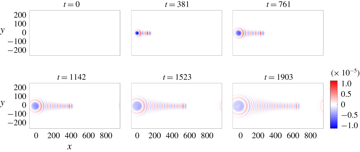
The evolution of the Lagrangian-mean velocity  $\overline{v}_{2}^{L}$ of the baroclinic mode for the resonant case. For reference,
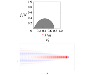
 $2\unicode[STIX]{x03C0}/(\unicode[STIX]{x1D707}kc_{g})\approx 363$. See also Movie 1 available at https://doi.org/10.1017/jfm.2020.82.

As expected from (3.10), figure 5 shows that the simulated  $\overline{v}_{2}^{L}$ is not confined to the region around the wavepacket. Instead, resonantly forced secondary waves are clearly seen to be shed behind the wavepacket. The dominant wavelength of the radiated secondary wavetrain can be estimated from (3.8a), (3.8b) and (3.8c) by matching its phase velocity with the group velocity of the primary wavepacket (see appendix B). This yields
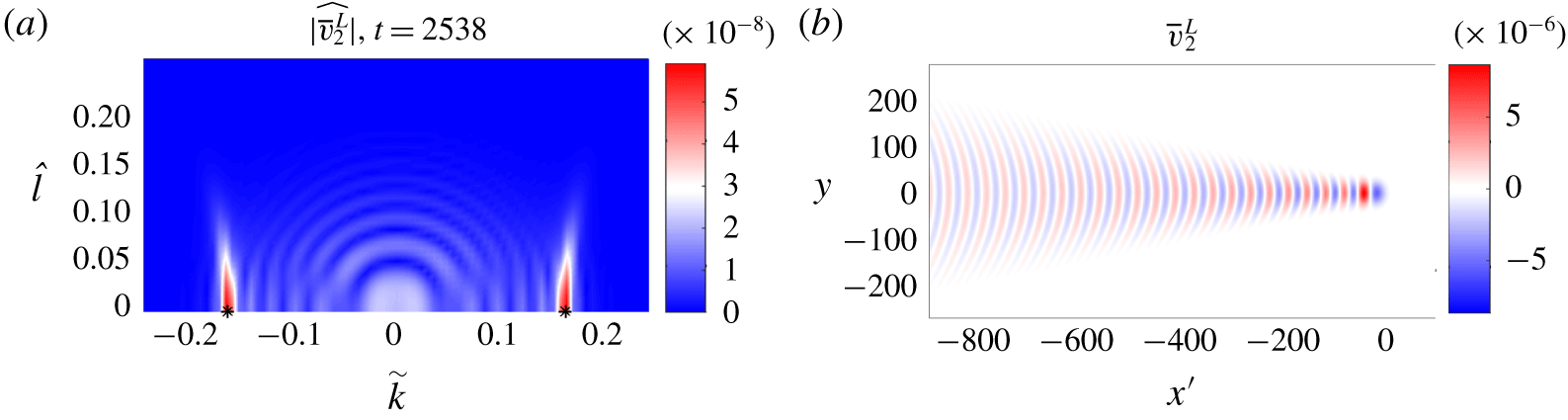
 $(\tilde{k},\tilde{l})=(\pm f/\sqrt{c_{g}^{2}-N^{2}/4m^{2}},0)\approx (\pm 0.17,0)$ for the dominant resonant modes. Figure 6(a) shows the absolute value of the wavenumber power spectrum of
 $\overline{v}_{2}^{L}$, i.e.
 $|\widehat{\overline{v}_{2}^{L}}|$ at the end of the simulation, where stars correspond to the predicted dominant modes. Thus, the numerical results are consistent with the Fourier analysis. We remark that the frequency of the dominant resonant mode is less than the central frequency of the wavepacket. Hence, the wave radiation transfers energy from higher to lower wave frequency.
(a) Absolute value of the wavenumber power spectrum of  $\overline{v}_{2}^{L}$ at the end of the simulation, which is at
 $t=2538\approx 14\unicode[STIX]{x03C0}/(\unicode[STIX]{x1D707}kc_{g})$. The stars mark the predicted dominant resonant modes,
 $(\tilde{k},\tilde{l})=(\pm f/\sqrt{c_{g}^{2}-N^{2}/4m^{2}},0)\approx (\pm 0.17,0)$. Panel (b) shows
 $\overline{v}_{2}^{L}$ computed by the damping method with
 $\unicode[STIX]{x1D700}=5\times 10^{-5}$ in the co-moving frame.

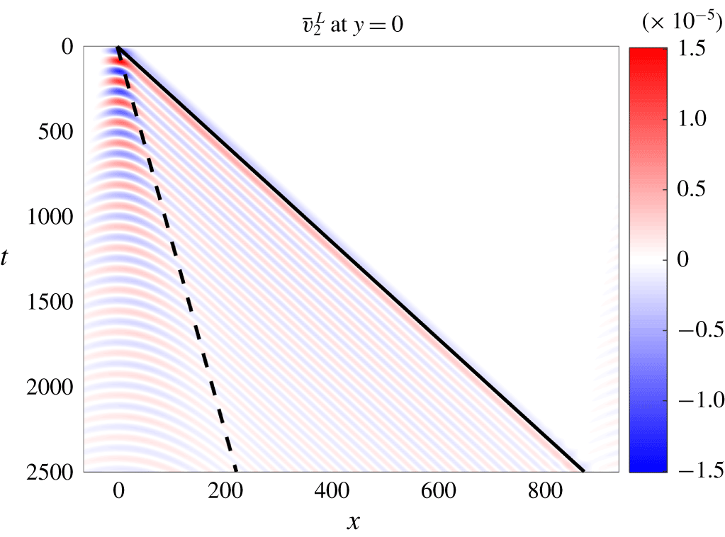
Numerically simulated  $\overline{v}_{2}^{L}$ at
 $y=0$ as a function of
 $(x,t)$ in the resonant regime. The black solid line denotes propagation with the wavepacket group velocity
 $c_{g}$ and the black dashed line denotes propagation with the group velocity
 $\overline{c}_{g}<c_{g}$ of the resonantly forced waves. The radiated waves are confined to the wedge-shaped area bounded by these lines.

The radiated wave solution in the co-moving frame can be computed by solving (3.9a) and (3.9b) without simulating the flows. However, a straightforward computation using the Fourier transforms of (3.9a) and (3.9b) runs into the usual problem with resonant waves: we find singularities for wavenumbers  $(\tilde{k},\tilde{l})$ satisfying
 $$\begin{eqnarray}c_{g}=\frac{1}{\tilde{k}^{2}}\left(\frac{N^{2}}{4m^{2}}(\tilde{k}^{2}+\tilde{l}^{2})+f^{2}\right).\end{eqnarray}$$
These singularities correspond to mean-flow wave modes with wavenumbers  $(\tilde{k},\tilde{l},2m)$ that satisfy the hydrostatic linear dispersion relation for co-moving solutions, i.e.
 $\unicode[STIX]{x1D714}^{2}=c_{g}^{2}\tilde{k}^{2}$. This is a common issue in radiation problems (e.g. Lighthill Reference Lighthill1978) and it results from the fact that the solution is not unique unless appropriate boundary conditions at infinity are specified, i.e. energy is only radiated from the wavepacket to infinity, and not the other way around. Lighthill (Reference Lighthill1978) (and recently Haney & Young (Reference Haney and Young2017)) use the method of slowly growing forcing to make the solution unique and obtain the desired solution by letting the growth rate go to zero. Here, we use a simpler method that works as well as the growing-forcing method.
We modify the solution by adding a small linear damping to (3.8a), (3.8b) and (3.8c). In particular, we replace  $\unicode[STIX]{x2202}_{t}^{2}$ by
 $\unicode[STIX]{x2202}_{t}^{2}+\unicode[STIX]{x1D700}\unicode[STIX]{x2202}_{t}$ and seek a steady solution in the co-moving frame. This solution decays at infinity for any positive
 $\unicode[STIX]{x1D700}>0$, i.e. it is a co-moving solution. As
 $\unicode[STIX]{x1D700}\rightarrow 0^{+}$, this solution then converges to the radiating solution in any bounded domain. Figure 6(b) shows the solution
 $\overline{v}_{2}^{L}$ for
 $\unicode[STIX]{x1D700}=5\times 10^{-5}$. This clearly shows the same pattern as the numerical solution. Finally, the horizontal group velocity of the radiated waves
 $\overline{c}_{g}=N^{2}/(4m^{2}c_{g})$ is positive, but always less than the wavepacket
 $c_{g}$ by the regime criterion. Therefore, in the
 $x$-direction the radiated waves are found between two fronts moving with these two group velocities; this is illustrated in figure 7.
4.4 The dependence of the Lagrangian baroclinic mode on wavenumber and rotation
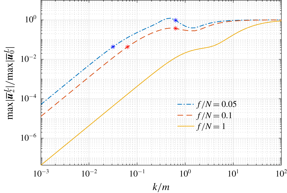
The demonstrated success of our analytical solutions allows for a wider investigation of parameter space, without the need for more direct numerical simulations. Here, thinking of the potential transport effects of resonating wavepackets in the ocean, we ask, how does the magnitude of the baroclinic Lagrangian-mean flow scale with the wave aspect and rotation-to-stratification ratios? Figure 8 shows  $\max |\overline{\boldsymbol{u}}_{2}^{L}|/\max |\overline{\boldsymbol{u}}_{0}^{L}|$ computed from theoretical solutions as a function of
 $k/m$ for
 $f/N=0.05$, 0.1 and 1. For any fixed
 $f/N$, when
 $k/m\rightarrow 0$, the baroclinic response becomes negligible. When
 $k/m\rightarrow \infty$, the magnitude of the baroclinic mode becomes equal to that of the barotropic mode, which has been shown in § 4.2.1. Thus, for a hydrostatic wavepacket, the baroclinic response is negligible, but for a non-hydrostatic wavepacket, the baroclinic mode is generally of equal importance relative to the barotropic mode. For relatively weak rotation rates, i.e.
 $f/N=0.05,0.1$, the resonant solutions connect continuously with the co-moving solutions, and there is a local minimum of
 $\max |\overline{\boldsymbol{u}}_{2}^{L}|/\max |\overline{\boldsymbol{u}}_{0}^{L}|$ near the transition from resonant solutions to co-moving solutions. When rotation is sufficiently strong, e.g.
 $f/N=1$, the resonant solutions do not exist. For fixed
 $k/m$, the relative magnitude of the baroclinic mode decreases with
 $f/N$.
The dependence of theoretical  $\max |\overline{\boldsymbol{u}}_{2}^{L}|/\max |\overline{\boldsymbol{u}}_{0}^{L}|$ on
 $k/m$ for
 $f/N=0.05$, 0.1 and 1. Points between the stars on the blue and red lines correspond to resonantly forced radiation solutions computed by the damping method, with
 $\unicode[STIX]{x1D700}=5\times 10^{-5}$.

5 Concluding comments
We have computed analytically the Lagrangian-mean motion induced by a vertically confined small-amplitude inertia–gravity wavepacket, in parameter regimes of relevance to the ocean, and demonstrated that the solutions are consistent with direct nonlinear numerical simulations of the Galerkin-truncated hydrostatic Boussinesq equations. The initial vertical wavenumber- $m$ packet excites a mean-flow response in modes
 $0$ and
 $2m$, the barotropic and baroclinic modes, respectively. The barotropic mean-flow response is characterized, for all parameters, by a co-moving Lagrangian-mean streamfunction, which is a new finding. The baroclinic mean-flow response, by contrast, exhibits two qualitatively different solution regimes – co-moving or radiating – with a transition between regimes that depends in a predictable way on the environmental parameters. This is also new.
The co-moving barotropic mean flow, determined here through a careful accounting of all the time-dependent wavepacket forcing terms, is reminiscent of the Bretherton flow of Reference BrethertonB69, owing its robust existence in part to the horizontal non-divergence of the barotropic mode, and to the three-dimensional setting of our problem; indeed, the barotropic flow disappears in the two-dimensional, vertical-slice setting of Reference BrethertonB69 and Van den Bremer et al. (Reference Van den Bremer, Yassin and Sutherland2019). For ocean-like parameters we found that the previously neglected barotropic flow actually dominates over the baroclinic response.
For the baroclinic mean flow, the criterion that decides between co-moving or radiating solutions follows from the hydrostatic dispersion relation for mean-flow waves in the form of (4.2). Specifically, a co-moving baroclinic response occurs only when the wavepacket group velocity magnitude  $|c_{g}|<N/(2m)$, a condition that arises again through inclusion of time-dependent forcing terms in the mean-flow response. Moreover, calculations indicated the presence of a non-negligible horizontal divergence in the induced baroclinic flow. Both features were supported by the numerical simulations. In the radiating regime, predicted to occur when
 $|c_{g}|>N/(2m)$, the baroclinic mean flow induces the radiation of resonantly forced inertia–gravity waves. These ‘mean-flow waves’ always travel at a slower group velocity than the primary wavepacket, resulting in the wake pattern behind the wavepacket depicted in figure 5. The excited modes seen in the numerical simulations are accurately predicted by the explicit calculation of this resonance in appendix B.
Wave radiation – or the non-existence of co-moving solutions – was also found by McIntyre (Reference McIntyre1973) and Van den Bremer et al. (Reference Van den Bremer, Yassin and Sutherland2019) in the non-rotating two-dimensional Boussinesq system, and by Reference Thomas, Buhler and SmithTBS18 in the shallow-water equations. However, wave radiation occurs only for a particular wavenumber in the non-rotating Boussinesq system, and only for  $f=0$ in the shallow-water system, results that suggest wave radiation is unlikely to occur in parameter regimes of relevance to the ocean. By contrast, our regime diagram in figure 1 shows that in the three-dimensional
 $f$-plane Boussinesq system, wave radiation occurs for a wide range of oceanically relevant parameters.
Finally, the radiated baroclinic waves continuously extract energy from the wavepacket. Because the frequency of the dominant resonantly forced waves is less than the central frequency of the wavepacket, this hints at a possible mechanism for spectral wave energy transfer towards lower frequencies for inertia–gravity waves in the ocean.
Acknowledgements
We thank the three referees for their constructive comments, which led to significant improvements of the manuscript. We also thank B. Young for discussions and suggesting the method underlying figure 6(b). O.B. gratefully acknowledges financial support from the United States National Science Foundation grants DMS-1312159 and DMS-1813891, and also Office of Naval Research grants N00014-15-1-2355 and N00014-19-1-2407. K.S.S. gratefully acknowledges financial support from United States National Aeronautical and Space Administration grant NNX16AJ35G, and from the New York University Abu Dhabi Institute.
Declaration of interests
The authors report no conflict of interest.
Supplementary movie
Supplementary movie is available at https://doi.org/10.1017/jfm.2020.82.
Appendix A. Derivation of (2.16)
We follow the steps in Wagner & Young (Reference Wagner and Young2015 to derive (2.16). The only difference in the proof is that we do not assume that the averaged wave interaction terms are time independent. Taking the scalar product of (2.5a) with  $\unicode[STIX]{x1D743}_{z}^{\prime }$, we have
 $$\begin{eqnarray}\overline{\unicode[STIX]{x1D743}_{z}^{\prime }\boldsymbol{\cdot }\boldsymbol{u}_{t}^{\prime }}+\overline{\unicode[STIX]{x1D743}_{z}^{\prime }\boldsymbol{\cdot }(f\boldsymbol{k}\times \boldsymbol{u}^{\prime })}+\overline{\unicode[STIX]{x1D743}_{z}^{\prime }\boldsymbol{\cdot }\unicode[STIX]{x1D735}P^{\prime }}-\overline{\unicode[STIX]{x1D701}_{z}^{\prime }b^{\prime }}=0.\end{eqnarray}$$
By the product rule,
 $$\begin{eqnarray}\overline{\unicode[STIX]{x1D743}_{z}^{\prime }\boldsymbol{\cdot }\boldsymbol{u}_{t}^{\prime }}=\unicode[STIX]{x2202}_{t}\overline{(\unicode[STIX]{x1D743}^{\prime }\boldsymbol{\cdot }\boldsymbol{u}^{\prime })}-{\textstyle \frac{1}{4}}\unicode[STIX]{x2202}_{z}\unicode[STIX]{x2202}_{t}^{2}\overline{\unicode[STIX]{x1D743}^{\prime 2}}+{\textstyle \frac{1}{2}}\unicode[STIX]{x2202}_{z}\overline{\boldsymbol{u}_{t}^{\prime }\boldsymbol{\cdot }\unicode[STIX]{x1D743}^{\prime }}.\end{eqnarray}$$
Similarly,
 $$\begin{eqnarray}\overline{\unicode[STIX]{x1D743}_{z}^{\prime }\boldsymbol{\cdot }(\boldsymbol{k}\times \boldsymbol{u}^{\prime })}={\textstyle \frac{1}{2}}\unicode[STIX]{x2202}_{z}\overline{(u^{\prime }\unicode[STIX]{x1D702}^{\prime }-v^{\prime }\unicode[STIX]{x1D709}^{\prime })}-{\textstyle \frac{1}{2}}\unicode[STIX]{x2202}_{t}\overline{(\unicode[STIX]{x1D709}_{z}^{\prime }\unicode[STIX]{x1D702}^{\prime }-\unicode[STIX]{x1D709}^{\prime }\unicode[STIX]{x1D702}_{z}^{\prime })}.\end{eqnarray}$$
Using  $b^{\prime }=-N^{2}\unicode[STIX]{x1D701}^{\prime }$, we have
 $-\overline{\unicode[STIX]{x1D701}^{\prime }b^{\prime }}=-\frac{1}{2}\unicode[STIX]{x2202}_{z}\overline{(\unicode[STIX]{x1D701}^{\prime }b^{\prime })}$. Substituting these terms into (A 1) and using the definitions of
 $p^{z}$ and
 $\overline{P}^{S}$, we have
 $$\begin{eqnarray}-\unicode[STIX]{x2202}_{t}p^{z}-{\textstyle \frac{1}{2}}\unicode[STIX]{x2202}_{z}\overline{P}^{S}+\overline{\unicode[STIX]{x1D743}^{\prime }\boldsymbol{\cdot }\unicode[STIX]{x1D735}P^{\prime }}-{\textstyle \frac{1}{4}}\unicode[STIX]{x2202}_{z}\unicode[STIX]{x2202}_{t}^{2}\overline{(\unicode[STIX]{x1D743}^{\prime 2})}=0.\end{eqnarray}$$
Finally, by the product rule,  $\unicode[STIX]{x2202}_{z}\overline{P}^{S}=\overline{\unicode[STIX]{x1D743}^{\prime }\boldsymbol{\cdot }\unicode[STIX]{x1D735}P^{\prime }}+\overline{P_{z}}^{S}$. Using this equation, (A 4) becomes
 $$\begin{eqnarray}\overline{P_{z}}^{S}={\textstyle \frac{1}{2}}\unicode[STIX]{x2202}_{z}\overline{P}^{S}-\unicode[STIX]{x2202}_{t}p^{z}-{\textstyle \frac{1}{4}}\unicode[STIX]{x2202}_{z}\unicode[STIX]{x2202}_{t}^{2}\overline{\unicode[STIX]{x1D743}^{\prime 2}},\end{eqnarray}$$
which is the vertical component of (2.16). The horizontal components of (2.16) can be derived analogously.
Appendix B. The resonant modes
In this appendix, we derive the equations for the wavenumbers of the resonant modes, and show that resonant modes grow linearly in time using the equation for the potential  $\unicode[STIX]{x1D719}_{2}$. Repeating the following process, the same conclusions follow for
 $\unicode[STIX]{x1D713}_{2}$ and
 $\tilde{b}$.
Defining the Fourier transform of  $\unicode[STIX]{x1D6F7}(x,y,t)$ as
 $$\begin{eqnarray}\widehat{\unicode[STIX]{x1D6F7}}(\tilde{k},\tilde{l},t)=\int \unicode[STIX]{x1D6F7}(x,y,t)\text{e}^{-\text{i}(\tilde{k}x+\tilde{l}y)}\,\text{d}x\,\text{d}y,\end{eqnarray}$$
the transform of (3.8a) yields
 $$\begin{eqnarray}\left[\unicode[STIX]{x2202}_{t}^{2}+f^{2}+\frac{N^{2}}{4m^{2}}\widetilde{k}^{2}+\frac{N^{2}}{4m^{2}}\widetilde{l}^{2}\right]\widehat{\unicode[STIX]{x1D719}_{2}}=\unicode[STIX]{x2202}_{t}^{2}\widehat{\unicode[STIX]{x1D719}^{\boldsymbol{p}}}+f\unicode[STIX]{x2202}_{t}\widehat{\unicode[STIX]{x1D713}^{\boldsymbol{p}}}-\unicode[STIX]{x2202}_{t}\widehat{G}.\end{eqnarray}$$
By the wavepacket approximation (2.7),
 $$\begin{eqnarray}\tilde{p}^{z}=\frac{1}{4}\frac{k\unicode[STIX]{x1D714}}{m^{2}}\left(\frac{m^{2}}{k^{2}}-1\right)a^{2}[A(\unicode[STIX]{x1D707}(x-c_{g}t),\unicode[STIX]{x1D707}y)]^{2},\quad \tilde{p}^{y}=0,\end{eqnarray}$$
and
 $$\begin{eqnarray}G=\frac{N^{2}}{8m^{2}}a^{2}[A(\unicode[STIX]{x1D707}(x-c_{g}t),\unicode[STIX]{x1D707}y)]^{2}.\end{eqnarray}$$
Using a change of variables and Fourier-transforming,
 $$\begin{eqnarray}\widehat{G}(\tilde{k},\tilde{l},t)=\frac{N^{2}}{8m^{2}}a^{2}\frac{1}{\unicode[STIX]{x1D707}^{2}}\widehat{A^{2}}(\tilde{k}/\unicode[STIX]{x1D707},\tilde{l}/\unicode[STIX]{x1D707})\text{e}^{-\text{i}\tilde{k}c_{g}t},\end{eqnarray}$$
which is a product of a function that depends on ( $\tilde{k},\tilde{l}$) and
 $\text{e}^{-\text{i}\tilde{k}c_{g}t}$. Similar expressions arise for
 $\tilde{\boldsymbol{p}}_{1}$,
 $\unicode[STIX]{x1D719}^{\boldsymbol{p}}$ and
 $\unicode[STIX]{x1D713}^{\boldsymbol{p}}$. Letting
 $$\begin{eqnarray}h=[-\tilde{k}^{2}c_{g}^{2}\widehat{\unicode[STIX]{x1D719}^{\boldsymbol{p}}}-\text{i}\tilde{k}c_{g}f\widehat{\unicode[STIX]{x1D713}^{\boldsymbol{p}}}-\text{i}\tilde{k}c_{g}{\hat{G}}]|_{t=0},\end{eqnarray}$$
equation (B 1) becomes
 $$\begin{eqnarray}\left[\unicode[STIX]{x2202}_{t}^{2}+f^{2}+\frac{N^{2}}{4m^{2}}\tilde{k}^{2}+\frac{N^{2}}{4m^{2}}\tilde{l}^{2}\right]\widehat{\unicode[STIX]{x1D719}_{2}}=h(\tilde{k},\tilde{l})\text{e}^{-\text{i}\tilde{k}c_{g}t}.\end{eqnarray}$$
Defining
 $$\begin{eqnarray}\unicode[STIX]{x1D6FA}(\tilde{k},\tilde{l})=\sqrt{f^{2}+\frac{N^{2}}{4m^{2}}(\tilde{k}^{2}+\tilde{l}^{2})}\end{eqnarray}$$
we find
 $$\begin{eqnarray}\widehat{\unicode[STIX]{x1D719}_{2}}=\left\{\begin{array}{@{}ll@{}}\displaystyle \frac{h}{2\text{i}\unicode[STIX]{x1D6FA}}\left(\frac{\text{e}^{-\text{i}\tilde{k}c_{g}t}-\text{e}^{\text{i}\unicode[STIX]{x1D6FA}t}}{-\text{i}(\unicode[STIX]{x1D6FA}+\tilde{k}c_{g})}-\frac{\text{e}^{-\text{i}\tilde{k}c_{g}t}-\text{e}^{-\text{i}\unicode[STIX]{x1D6FA}t}}{\text{i}(\unicode[STIX]{x1D6FA}-\tilde{k}c_{g})}\right)\quad & |\tilde{k}c_{g}|\neq \unicode[STIX]{x1D6FA},\\ \displaystyle \frac{h}{2\text{i}\unicode[STIX]{x1D6FA}}\left(\frac{\text{e}^{-\text{i}\unicode[STIX]{x1D6FA}t}-\text{e}^{\text{i}\unicode[STIX]{x1D6FA}t}}{-2\text{i}\unicode[STIX]{x1D6FA}}-t\text{e}^{-\text{i}\unicode[STIX]{x1D6FA}t}\right)\quad & \tilde{k}c_{g}=\unicode[STIX]{x1D6FA},\\ \displaystyle \frac{h}{2\text{i}\unicode[STIX]{x1D6FA}}\left(t\text{e}^{\text{i}\unicode[STIX]{x1D6FA}}-\frac{\text{e}^{\text{i}\unicode[STIX]{x1D6FA}t}-\text{e}^{-\text{i}\unicode[STIX]{x1D6FA}t}}{2\text{i}\unicode[STIX]{x1D6FA}}\right)\quad & -\tilde{k}c_{g}=\unicode[STIX]{x1D6FA}.\end{array}\right.\end{eqnarray}$$
Thus, when  $|\tilde{k}c_{g}|\neq \unicode[STIX]{x1D6FA}$,
 $\widehat{\unicode[STIX]{x1D719}}_{2}$ is a linear combination of oscillators in time. When
 $|\tilde{k}c_{g}|=\unicode[STIX]{x1D6FA}$,
 $\widehat{\unicode[STIX]{x1D719}}_{2}$ consists of two oscillations with the same frequency, and the amplitude of one of the oscillations grows linearly in time. For large
 $t$,
 $\widehat{\unicode[STIX]{x1D719}}_{2}$ grows approximately linearly. Resonant modes satisfy
 $\unicode[STIX]{x1D6FA}^{2}=\tilde{k}^{2}c_{g}^{2}$, i.e.
 $$\begin{eqnarray}\left(c_{g}^{2}-\frac{N^{2}}{4m^{2}}\right)\tilde{k}^{2}-\frac{N^{2}}{4m^{2}}\tilde{l}^{2}=f^{2}.\end{eqnarray}$$
The smallest wavenumber satisfying this equation is  $(f/\sqrt{c_{g}^{2}-N^{2}/4m^{2}},0)$. Since
 $A$ is a Gaussian function,
 $\widehat{A^{2}}$ is also Gaussian. By (B 4) and the definition of
 $h$ in (B 5),
 $h(\tilde{k},\tilde{l})$ is likely to reach its maximum at
 $(\pm f/\sqrt{c_{g}^{2}-N^{2}/4m^{2}},0)$ and the dominant mode of
 $\widehat{\unicode[STIX]{x1D719}}$ is likely to occur at
 $(\pm f/\sqrt{c_{g}^{2}-N^{2}/4m^{2}},0)$. These predictions are verified in § 4.
Appendix C. The Galerkin-truncated hydrostatic Boussinesq equations
With no-flux and free-slip vertical boundary conditions, the solutions of the  $f$-plane Boussinesq equations can be written as trigonometric series in
 $z$. Keeping three vertical modes, we write the field variables as
 $$\begin{eqnarray}\displaystyle & \displaystyle (u,v,P)=(u_{0},v_{0},P_{0})+(u_{1},v_{1},P_{1})\cos (mz)+(u_{2},v_{2},P_{2})\cos (2mz), & \displaystyle\end{eqnarray}$$
 $$\begin{eqnarray}\displaystyle & \displaystyle (w,b)=(w_{1},b_{1})\sin (mz)+(w_{2},b_{2})\sin (2mz), & \displaystyle\end{eqnarray}$$
where the subscript 0 corresponds to the barotropic mode, 1 corresponds to the first baroclinic mode and 2 corresponds to the second baroclinic mode. Substituting these truncated solutions into the hydrostatic Boussinesq equations, we obtain the governing equations for the three modes. In the following, the vector velocities are to be taken as their horizontal components, e.g.  $\boldsymbol{u}=(u,v)$.
The barotropic mode equations are
 $$\begin{eqnarray}\displaystyle & & \displaystyle \unicode[STIX]{x2202}_{t}\boldsymbol{u}_{0}+f\hat{\boldsymbol{z}}\times \boldsymbol{u}_{0}+\unicode[STIX]{x1D735}_{h}P_{0}+\boldsymbol{u}_{0}\boldsymbol{\cdot }\unicode[STIX]{x1D735}_{h}\boldsymbol{u}_{0}\nonumber\\ \displaystyle & & \displaystyle \quad +\,{\textstyle \frac{1}{2}}(\boldsymbol{u}_{1}\boldsymbol{\cdot }\unicode[STIX]{x1D735}_{h}\boldsymbol{u}_{1}+\boldsymbol{u}_{2}\boldsymbol{\cdot }\unicode[STIX]{x1D735}_{h}\boldsymbol{u}_{2}-mw_{1}\boldsymbol{u}_{1}-2mw_{2}\boldsymbol{u}_{2})=0,\end{eqnarray}$$
 $$\begin{eqnarray}\unicode[STIX]{x1D735}_{h}\boldsymbol{\cdot }\boldsymbol{u}_{0}=0.\end{eqnarray}$$
The first baroclinic mode equations are
 $$\begin{eqnarray}\displaystyle & & \displaystyle \unicode[STIX]{x2202}_{t}\boldsymbol{u}_{1}+f\hat{\boldsymbol{z}}\times \boldsymbol{u}_{1}+\unicode[STIX]{x1D735}_{h}P_{1}+\boldsymbol{u}_{1}\boldsymbol{\cdot }\unicode[STIX]{x1D735}_{h}\boldsymbol{u}_{0}+\boldsymbol{u}_{0}\boldsymbol{\cdot }\unicode[STIX]{x1D735}_{h}\boldsymbol{u}_{1}\nonumber\\ \displaystyle & & \displaystyle \quad +\,{\textstyle \frac{1}{2}}(\boldsymbol{u}_{2}\boldsymbol{\cdot }\unicode[STIX]{x1D735}_{h}\boldsymbol{u}_{1}+\boldsymbol{u}_{1}\boldsymbol{\cdot }\unicode[STIX]{x1D735}_{h}\boldsymbol{u}_{2})-{\textstyle \frac{1}{2}}(mw_{2}\boldsymbol{u}_{1}+2mw_{1}\boldsymbol{u}_{2})=0,\end{eqnarray}$$
 $$\begin{eqnarray}\displaystyle & \displaystyle \unicode[STIX]{x1D735}_{h}\boldsymbol{\cdot }\boldsymbol{u}_{1}+mw_{1}=0, & \displaystyle\end{eqnarray}$$
 $$\begin{eqnarray}\displaystyle & \displaystyle mP_{1}+b_{1}=0, & \displaystyle\end{eqnarray}$$
 $$\begin{eqnarray}\displaystyle & & \displaystyle \unicode[STIX]{x2202}_{t}b_{1}+N^{2}w_{1}+\boldsymbol{u}_{0}\boldsymbol{\cdot }\unicode[STIX]{x1D735}_{h}b_{1}\nonumber\\ \displaystyle & & \displaystyle \quad +\,{\textstyle \frac{1}{2}}(\boldsymbol{u}_{1}\boldsymbol{\cdot }\unicode[STIX]{x1D735}_{h}b_{2}-\boldsymbol{u}_{2}\boldsymbol{\cdot }\unicode[STIX]{x1D735}_{h}b_{2})+{\textstyle \frac{1}{2}}(mw_{2}b_{1}-2mw_{1}b_{2})=0.\end{eqnarray}$$
And finally, the second baroclinic mode equations are
 $$\begin{eqnarray}\displaystyle & & \displaystyle \unicode[STIX]{x2202}_{t}\boldsymbol{u}_{2}+f\hat{\boldsymbol{z}}\times \boldsymbol{u}_{2}+\unicode[STIX]{x1D735}_{h}P_{2}+\boldsymbol{u}_{0}\boldsymbol{\cdot }\unicode[STIX]{x1D735}_{h}\boldsymbol{u}_{2}+\boldsymbol{u}_{2}\boldsymbol{\cdot }\unicode[STIX]{x1D735}_{h}\boldsymbol{u}_{0}\nonumber\\ \displaystyle & & \displaystyle \quad +\,{\textstyle \frac{1}{2}}\boldsymbol{u}_{1}\boldsymbol{\cdot }\unicode[STIX]{x1D735}_{h}\boldsymbol{u}_{1}+{\textstyle \frac{1}{2}}mw_{1}\boldsymbol{u}_{1}=0,\end{eqnarray}$$
 $$\begin{eqnarray}\displaystyle & \displaystyle \unicode[STIX]{x1D735}_{h}\boldsymbol{\cdot }\boldsymbol{u}_{2}+2mw_{2}=0, & \displaystyle\end{eqnarray}$$
 $$\begin{eqnarray}\displaystyle & \displaystyle 2mP_{2}+b_{2}=0, & \displaystyle\end{eqnarray}$$
 $$\begin{eqnarray}\displaystyle & \displaystyle \unicode[STIX]{x2202}_{t}b_{2}+N^{2}w_{2}+\boldsymbol{u}_{0}\boldsymbol{\cdot }\unicode[STIX]{x1D735}_{h}b_{2}+{\textstyle \frac{1}{2}}(\boldsymbol{u}_{1}\boldsymbol{\cdot }\unicode[STIX]{x1D735}_{h}b_{1}+mw_{1}b_{1})=0. & \displaystyle\end{eqnarray}$$
Appendix D. ‘Now-casting’ the linear displacement fields for plane waves in a vertically bounded domain
The accurate computation of Stokes corrections and the Lagrangian pseudomomentum vector field requires knowledge of the wave-induced linear particle displacement fields, which are, however, not available from a standard Eulerian numerical scheme. At small wave amplitude, the displacement fields associated with inertia–gravity waves can be computed from a single snapshot of the velocity and buoyancy fields. The direct approach for doing this is to decompose the flow variables into waves and balanced geostrophic flow components, and then to compute the linear particle displacements for each wave mode in spectral space. However, for a single baroclinic mode of the hydrostatic Boussinesq equations, a shortcut is possible that greatly simplifies this computation.
The linear particle displacements  $\unicode[STIX]{x1D743}=(\unicode[STIX]{x1D709},\unicode[STIX]{x1D702},\unicode[STIX]{x1D701})$ have the modal representation
 $$\begin{eqnarray}(\unicode[STIX]{x1D709},\unicode[STIX]{x1D702})=(\unicode[STIX]{x1D709}_{1},\unicode[STIX]{x1D702}_{1})\cos mz\quad \text{and}\quad \unicode[STIX]{x1D701}=\unicode[STIX]{x1D701}_{1}\sin mz,\end{eqnarray}$$
where  $(\unicode[STIX]{x1D709}_{1},\unicode[STIX]{x1D702}_{1},\unicode[STIX]{x1D701}_{1})$ are functions of
 $(x,y,t)$. The vertical
 $\unicode[STIX]{x1D701}_{1}$ follows from incompressibility as
 $\unicode[STIX]{x1D701}_{1}=-(1/m)(\unicode[STIX]{x1D709}_{1,x}+\unicode[STIX]{x1D702}_{1,y})$, hence, it suffices to find the horizontal displacement fields. In a Helmholtz decomposition
 $$\begin{eqnarray}\unicode[STIX]{x1D709}_{1}=A_{x}-B_{y}\quad \text{and}\quad \unicode[STIX]{x1D702}_{1}=A_{y}+B_{x},\end{eqnarray}$$
the fields  $A(x,y,t)$ and
 $B(x,y,t)$ are the potential and streamfunctions for
 $(\unicode[STIX]{x1D709}_{1},\unicode[STIX]{x1D702}_{1})$. Taking the vertical curl and horizontal divergence of the linear horizontal momentum equations yields
 $$\begin{eqnarray}\unicode[STIX]{x1D6FB}_{h}^{2}B_{tt}+f(u_{1,x}+v_{1,y})=0,\end{eqnarray}$$
and
 $$\begin{eqnarray}\unicode[STIX]{x1D6FB}_{h}^{2}A_{tt}=f(v_{1,x}-u_{1,y})+\frac{1}{m}\unicode[STIX]{x1D6FB}_{h}^{2}b_{1},\end{eqnarray}$$
after using the modal hydrostatic relation  $-mP_{1}=b_{1}$. Note that the geostrophic component makes no contribution to the horizontal flow divergence, so (D 3) can be used to diagnose
 $B$ directly from the numerical
 $(u_{1},v_{1})$ after taking horizontal Fourier transforms and then replacing
 $\unicode[STIX]{x2202}_{t}^{2}$ by
 $-\unicode[STIX]{x1D714}^{2}$ from the dispersion relation. For (D 4), it seems inevitable to subtract the balanced flow component first before trying to compute
 $A$, but in fact this is not the case. To see this we look at the mode-
 $m$ linear potential vorticity and quasi-geostrophic streamfunction
 $\unicode[STIX]{x1D713}^{G}$ such that
 $$\begin{eqnarray}q_{1}=v_{1,x}-u_{1,y}+\frac{fm}{N^{2}}b_{1}=\left(\unicode[STIX]{x1D6FB}_{h}^{2}-\frac{f^{2}m^{2}}{N^{2}}\right)\unicode[STIX]{x1D713}^{G}.\end{eqnarray}$$
The geostrophic fields are linked to  $\unicode[STIX]{x1D713}^{G}$ by the usual relations
 $$\begin{eqnarray}u_{1}^{G}=-\unicode[STIX]{x1D713}_{y}^{G},\quad v_{1}^{G}=+\unicode[STIX]{x1D713}_{x}^{G},\quad \text{and}\quad b_{1}^{G}=-mf\unicode[STIX]{x1D713}^{G}.\end{eqnarray}$$
Now, substituting these fields into the right-hand side of (D 4) yields zero, so we do not need to subtract the balanced fields before using (D 4) to diagnose  $A$.