

Introduction
The United States National Snow and Ice Data Center (NSIDC) manages an expanding collection of almost 600cryospheric and related data sets. Based on statistics from the fiscal year 2005, the research and higher edu-cation community is the primary data user group, comprising 63.27 of all users (NSIDC 2005). As new data access and visualisation technologies emerge, opportu-nities arise to make data available to new users and applications. Google™ has modified the way in which people visualise spatial data. There have been 100million installations of the Google Earth™ application since the release of Google Earth in June 2005 (Geography 2006). Google Earth provides a user-friendly environment for the visualisation of the Earth in a simple intuitive manner. This paper presents a project focusing on the creation of an XML-based compressed Keyhole Markup Language (KMZ) file that highlights glacier photographs, permafrost type and extent, sea ice concentration and extent, and snow extent. The NSIDC created file is entitled ‘Snow, ice, glaciers and permafrost file for Google Earth’ and is available for download (NSIDC 2007). The ubiquity of Google Earth, the free software download and the ease of use led us to experiment with making polar data available in Google Earth.
There are many Keyhole Markup Language (KML) files distributed on the web that contain cryospheric images. For example, the ‘Developing Arctic Modelling and Observing Capabilities for Long-term Environmental Studies’ (DAMOCLES) Google Earth project (Technical University of Denmark 2006), encompasses sea ice and related products while the National Operational Hydro-logic Remote Sensing Center (NOHRSC 2006) distri-butes KML files with snow reports and analyses overlays. The DAMOCLES file contains a suite of cryospheric data overlaid in Google Earth, including sea ice concentra-tion, ice motion, and tracks of buoys, ships, and drifting stations. NOHRSC creates new files daily for users to view current snow reports and analyses. While these two projects emphasise the individual parameters of sea ice and snow cover, the project at NSIDC offers a more com-prehensive view of the cryosphere, combining images representing four major components of the cryosphere, (glaciers, permafrost, sea ice, and snow) and distributing them as one KMZ file.
We seek to expand the understanding and use of our data, but making images visible in Google Earth may also improve data availability because investigators see the outreach benefit of making data available through that medium. For example, the Royal Netherlands Institute for Sea Research has found that some data providers will make their data available sooner when they can see how data access can be enhanced with tools such as Google Earth (T. de Bruin, personal communication, April 2006). Overall, Google Earth and similar virtual globe technologies promise exciting and dynamic ways to present data and imagery that may enhance data availability, understanding, and access.
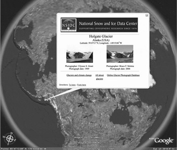
A pop-up displaying Holgate Glacier, Alaska, taken in 1909 by Ulysses S. Grant and in 2004 by Bruce F. Molnia.

Cryospheric products
For this trial project, three products distributed by NSIDC were selected; the Online Glacier Photograph Database, the Circum-Arctic Map of Permafrost and Ground-Ice Conditions, and the Near Real-Time SSM/I Equal-area Scalable Earth Grid (EASE-Grid) Daily Global Ice Concentration and Snow Extent (NSIDC/WDC 2006; Brown and others Reference Brown, Ferrians, Heginbottom and Melnikov1998; Nolin and others Reference Nolin, Armstrong and Maslanik1998). These products do not represent the entire cryosphere, but relate to a significant portion of it. This section describes the original input products used to create the KMZ file.
The Online Glacier Photograph Database comprises more than 3,000 glacier photographs extending from the 1880s to 2004, primarily covering the northwest United States and Alaska (NSIDC/WDC 2006). Photographs in the collection were taken on the ground and from the air. Within the collection there are 14 repeat photographs of Alaskan glaciers. The repeat photography reveals how each glacier terminus has retreated over time. Fig. 1 highlights the repeat photography by showing side by side images of Holgate Glacier, Alaska, taken in 1909 by Ulysses S. Grant and in 2004 by Bruce F. Molnia.
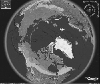
The Circum-Arctic Map of Permafrost and Ground-Ice Conditions data set spans the northern hemisphere from 25° N to 90° N and delineates continuous, discontinuous, sporadic and isolated permafrost regions as well as relict and subsea permafrost boundaries (Brown and others Reference Brown, Ferrians, Heginbottom and Melnikov1998). Relict permafrost is permafrost existing in areas where permafrost cannot form under present climatic conditions. Subsea permafrost is permafrost occurring beneath the sea bottom. It may be a result of sub-zero saline water temperatures or may be relict permafrost (Everdingen Reference Everdingen1998). The data set consists of shapefiles derived from the original 1:10,000,000 paper map (Brown and others Reference Brown, Ferrians, Heginbottom and Melnikov1997). Fig. 2 displays the permafrost image overlay in Google Earth.
Example of how permafrost appears in Google Earth.

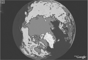
The Near Real-Time SSM/I EASE-Grid Daily Global Ice Concentration and Snow Extent data set (Nolin and others Reference Nolin, Armstrong and Maslanik1998) consists of near real-time data derived from the Defense Meteorological Satellite Program (DMSP) F-13 Special Sensor Microwave/Imager (SSM/I). See Fig. 3 for an example of the snow and ice layer in Google Earth. NSIDC produces and posts daily a new image to the NSIDC Web site. The KMZ file references the image on the NSIDC web site. Therefore, on any day that the KMZ file is opened in Google Earth, the most recent sea ice and snow image appears. This ‘dynamic’ approach provides a current view of sea ice and snow data without having to download a separate KMZ file.
A sample image of the snow and ice coverage.

Methodology
This section describes the processing steps taken for each of the three products, which primarily consists of converting the data into images that are compatible with Google Earth. Google Earth only displays files in JPG, PNG, GIF, or TIFF formats (Google Earth 2006). Google Earth displays GeoTIFF images but ignores the projection information and handles them as TIFF images. The process of converting data to these formats varies by product.
To be compatible with Google Earth, all images must be in a cylindrical equidistant projection (Google Earth 2006). The most commonly used cylindrical equidistant projection is the Equatorial Cylindrical Equidistant (also known as: simple cylindrical, geographic, latitude/longitude, platte-caree, Cartesian, etc.), which uses the equator as the reference latitude. For polar data the authors have found that using a reference latitude in the same region as the data makes the image overlay look better in Google Earth. By describing our approach in detail we highlight certain issues and requirements, especially when working with polar data.
Glacier photographs
The metadata for the glacier photographs are stored in a database at NSIDC. The key attributes selected to appear in Google Earth include the glacier photograph identifier, glacier name, photographer name, latitude and longitude. To incorporate the metadata into the proper KML format based on guidelines in the KML specifications (Google Earth 2006), a Perl script was written to convert the metadata values for approximately 3,000 photographs into the KML format. This resulted in a very large KML file, almost 2,000 pages in length. This material was condensed and it now contains almost 1,500 pages of code. Due to the large file size, the KML file was compressed into a KMZ file. The results place push-pins on the Earth for each glacier location. By clicking on the link for a selected glacier photograph, a pop-up picture of each glacier photograph appears along with relevant links to the NSIDC Web site.
Permafrost image
The digital permafrost shapefiles were derived from a paper map with a scale of 1:10,000,000. According to Tobler (Reference Tobler and Mounsey1988), this suggests an approximate spatial resolution of 5 km for the paper map. A representative fraction (for example 1:10,000,000), however, is not an appropriate way to describe the level of geographic detail for a digital data set (Goodchild and Proctor Reference Goodchild and Proctor1997). Furthermore, the paper map was derived from a variety of sources with varying resolutions (Heginbottom and others Reference Heginbottom, Brown, Melnikov and Ferrians1993), and some of the polygons in this product represent permafrost areas as small as three hundred meters.
Using ArcGIS™9, the individual permafrost shape-files were reprojected into a cylindrical equidistant pro-jection. The various layers (separate layers for subsea, continuous, etc.) were overlain together in one map (.mxd) file and then exported as a 600 dpi Portable Network Graphics (PNG) image. At this stage, areas that were not underlain by permafrost were displayed as a solid white colour. ImageMagick software was used to make these white areas transparent (ImageMagick 2006).
A 600 dpi resolution was chosen for the image (6381 × 1182 pixels) as a reasonable compromise that did not lead to an unduly large file, but also appeared reasonably attractive in Google Earth (not too blocky). It is important to note that this is an image overlay and not the actual data, yet it is interesting to contrast the image resolution with the resolution of the data. The 600 dpi image has an approximate resolution of 0.05 degrees or about 6 km north/south (and variable east/west becoming increasingly finer toward the pole).
Ice and snow image
The ice and snow image referenced in this project is recreated daily from remotely sensed SSM/I data in binary (2-byte integers) format. It should be noted that the ice and snow image combines the sea ice concentration and extent and snow extent parameters into one image. The original data files are hemispheric, meaning there is one file for the northern hemisphere and one for the southern hemisphere. The hemispheric data files are distributed in a polar azimuthal projection at a 25 km ground resolution that contains a mask for land, oceans, lakes, coastlines, and the ‘pole-hole’ where the SSM/I sensor does not actually collect data directly at the poles due to the near polar orbit.
The hemispheric data files are regridded, using the Mapx (Geospatial Methods 2007) map transformations library, into quarter degree cylindrical equidistant grids. Each data grid is then converted to an image format and NetPBM tools (NetPBM 2006) are used for further image manipulation. The separate northern and southern images are joined, and the northern ‘pole-hole’ is filled in since we infer that this area is underlain with sea ice.
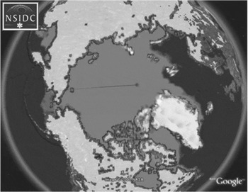
When the authors initially displayed the resulting image overlays in Google Earth 3, seam lines were apparent along the international dateline. Fig. 4 shows an example. To overcome this problem, an overlap region was created by increasing the width of the image one degree (four pixels) on either side. This created a longitude range for the image of [−181, 181] and prevented the dateline seam in the overlay.
Example of ice and snow image with a seam along the dateline.

When Google Earth version 4 was released in beta the authors started experimenting with it and discovered that the overlap region at the dateline was displayed as a darker colour than elsewhere on many platforms. It was decided to revert to the original longitude range of [−180, 180]. Fortunately Google Earth version 4.0.2737 appears to have fixed the problem with the seam at the dateline on most platforms so that whole issue may be resolved. The final step in the process is to make areas of the image that are not snow or ice transparent, so the default data in Google Earth can show through, and convert the image to PNG format.
Results and discussion
From 15 March 2006 to 31 January 2007, the NSIDC KMZ file was downloaded 3,353 times by 2,554 unique IP addresses, excluding NSIDC IP addresses and well-known robots. Data users were primarily interested in seeing images and data in Google Earth and understanding how the KMZ file was created. Colleagues at scientific conferences, such as the autumn American Geophysical Union (AGU) meeting, have recommended that the Google Earth work be conveyed to universities, as the material has potential value in education. Other feedback suggests that including sea ice images from previous years would be beneficial for comparative purposes. In this context it should be noted that the authors have begun making a monthly time series of sea ice images available.
The primary challenges with this project include the initial learning curve with the KML syntax, how to handle the now-resolved dateline issue, and making the values not snow or ice transparent. One continuing challenge is that the technology changes so quickly, as the work with the dateline seam demonstrates. The aim is to keep up with the changes and to produce workarounds to handle problems as they emerge. Often the problems with the Google Earth software are resolved later on and the workarounds require retraction. Once the entire process of converting data and creating the KMZ file is established, these challenges become easier to address for other data sets. It would be a very cumbersome process, however, to include every NSIDC data set in Google Earth because of the large volume of data, the varying product formats, and the manual effort that would be required for each of the data conversions.
In the short term, the manageability of the NSIDC KMZ file needs to be addressed, since the file contains almost 1,500 pages of KML code. For future updates or additions, the best solution may be to separate each product into a separate KMZ file rather than compiling them together. Pointers in a KML file could be used to reference other KML or KMZ files posted on a web site (Google Earth 2006). For example, each data set could be partitioned into a separate KML or KMZ file, the new files could be posted to the web site, and pointers in one comprehensive KML file could point to each individual KML or KMZ file. These changes could improve maintenance issues for future updates.
Conclusion
The popularity of Google Earth suggests that there is a great interest in using the tool to explore the Earth's geography. Google Earth offers a rich and compelling means of viewing the Earth. Students and educators as well as the broader public can use the tool to gain a better perspective on geographic phenomena. This improved perspective can only benefit the Earth sciences. It is particularly valuable for the polar regions, which are often poorly represented on two-dimensional world maps. Meanwhile, scientists appreciate the outreach possibilities of making data viewable in Google Earth and are beginning to explore actual scientific applications for the tool.
The experiment described in this paper of making cryospheric data available shows the potential for using Google Earth as a means to display representative scientific data and imagery. The tool will need to continue to evolve, however, if it is to provide more scientific functionality than simple exploration and browse capabilities. A major value of the tool is that it allows for an interactive 3D perspective. However, the mechanisms for making data and imagery viewable are still oriented towards a simple two-dimensional Cartesian representation of the Earth. Reprojecting polar data to a cylindrical equidistant projection makes little sense scientifically, and the process can affect the resolution, accuracy, and display of the data.
In this context, it is important to make a clear distinction between the inclusion of actual data in Google Earth (such as air temperatures at given points or the photographs of glaciers) and representative imagery derived from the data (such as the permafrost and snow and ice overlays). While the display of the images enables browsing of the data and provides perspective on geographic phenomena, it does not yet allow for scientific analysis. It may be beyond the scope of Google Earth to be a scientific analysis tool, but this may be a possibility in the future. For example, it is now possible to view animated time series of images in Google Earth. NSIDC has recently taken advantage of this feature by displaying a 28-year time series of monthly sea ice extent, illustrating the recent decline of Arctic sea ice. Google Earth could be even more scientifically useful if it accommodated richer and more diverse data structures and formats and improved its representation of scale and resolution.
NSIDC's initial experience working with Google Earth shows great promise. It is not difficult to make data and imagery viewable in Google Earth, but the constraints of KML encoding can be somewhat cumbersome. Having now surmounted the initial learning curve, NSIDC is exploring new ways to use Google Earth to improve the accessibility, understanding, and usability of its data. Google Earth and related virtual globe technology are rapidly improving, and we anticipate even broader application by both scientists and non-scientists.
Acknowledgements
The authors express gratitude to Mary Jo Brodzik, Jennifer Bohlander, Richard Armstrong and Clark Judy for their support, scientific and/or technical expertise, which was needed and much appreciated. We would also like to thank Florence Fetterer and Jane Beitler for reviewing early versions of this paper and Beth Kumar for providing final edits. In addition, we want to express thanks to Ken Dean and an anonymous reviewer for their constructive feedback. This work was funded in part by NOAA NESDIS [NOAA Cooperative Agreement NA17RJ1229].