A hybrid numerical model for the collective motion of fish groups

Xuewei Mao; Jiadong Wang; Xingyuan Mao; Jian Deng

doi:10.1017/jfm.2025.216

A hybrid numerical model for the collective motion of fish groups

Published online by Cambridge University Press: 14 April 2025

Xingyuan Mao and

Xuewei Mao: Affiliation:
State Key Laboratory of Fluid Power and Mechatronic Systems, Department of Mechanics, Zhejiang University, Hangzhou 310027, PR China
Jiadong Wang: Affiliation:
State Key Laboratory of Fluid Power and Mechatronic Systems, Department of Mechanics, Zhejiang University, Hangzhou 310027, PR China
Xingyuan Mao: Affiliation:
State Key Laboratory of Fluid Power and Mechatronic Systems, Department of Mechanics, Zhejiang University, Hangzhou 310027, PR China
Jian Deng*: Affiliation:
State Key Laboratory of Fluid Power and Mechatronic Systems, Department of Mechanics, Zhejiang University, Hangzhou 310027, PR China
*: Corresponding author: Jian Deng, zjudengjian@zju.edu.cn

Article contents

Abstract
Introduction
Methodology
Sensitivity study and verification of the numerical models
Results and discussion
Conclusions
Supplementary movies
Funding
Declaration of interests
References

Rights & Permissions

Abstract

We propose a hybrid numerical model for the collective motion of fish groups, which integrates an agent-based model with a computational fluid dynamics (CFD)-based model. In the agent-based model, the fish group is represented by self-propelled particles (SPPs), incorporating social forces with local interactive rules. The CFD-based model treats the fish body with an undulated filament that responds to the hydrodynamic forces imposed by the surrounding fluid flow. These two models are coupled using a central pattern generator controller. We test this hybrid model with groups of 30–50 individuals. The results show that the group exhibits various collective behaviours, including tight schooling, sparse schooling and milling patterns, by adjusting the coefficients in the SPP model. Due to the hydrodynamic interactions, particularly with the obstacle avoidance model, both the individuals’ and the group’s mean speed fluctuate, differentiating it from traditional SPP models that typically consider volumeless particles. More interestingly, our findings indicate that fish benefit from collective motion in terms of energetic consumption in both schooling and milling patterns. It is important to note that the swimming fish are actuated using a very simple mechanism without any optimisation strategy. An additional study investigates the effects of the Reynolds number, demonstrating the capability of the current hybrid model to account for fish groups of varying body lengths or swimming speeds. Future applications of this model are promising, offering potential insights into the energetic advantages of collective motion in large-scale fish groups.

JFM classification

Biological Fluid Dynamics: Collective behaviour Biological Fluid Dynamics: Swimming/flying Biological Fluid Dynamics: Propulsion

Information

Type: JFM Papers
Information: Journal of Fluid Mechanics , Volume 1009 , 10 May 2025, A26
DOI: https://doi.org/10.1017/jfm.2025.216 [Opens in a new window]
Copyright: © The Author(s), 2025. Published by Cambridge University Press

1. Introduction

Collective behaviour is a widespread phenomenon observed across various animal groups, including army ant colonies, zebra herds, starling flocks and schools of sardines. The coordinated motion of individuals within these groups is believed to confer several advantages (Krebs, MacRoberts & Cullen Reference Krebs, MacRoberts and Cullen1972; Lazarus Reference Lazarus1979; Landeau & Terborgh Reference Landeau and Terborgh1986; Romanczuk, Couzin & Schimansky-Geier Reference Romanczuk, Couzin and Schimansky-Geier2009; Ioannou, Guttal & Couzin Reference Ioannou, Guttal and Couzin2012; Bastien & Romanczuk Reference Bastien and Romanczuk2020). Among these groups, fish schools play a particularly crucial role in nature, fulfilling multiple biological functions, including reducing predation risk (Brock & Riffenburgh Reference Brock and Riffenburgh1960; Cushing & Jones Reference Cushing and Jones1968; Deng & Liu Reference Deng and Liu2021), amplifying feeding and reproductive opportunities (Pitcher, Magurran & Winfield Reference Pitcher, Magurran and Winfield1982) and minimising energy expenditure (Weihs Reference Weihs1973).

To gain a comprehensive understanding of the complexities and principles behind schooling behaviours, various numerical methods have emerged. Broadly, these can be classified into agent-based models and computational fluid dynamics (CFD) simulations. Agent-based algorithms capture collective movements by employing social forces that simulate individual behaviours, often overlooking the intricate interactions between individuals and their fluid environment. Such models have significantly contributed to our understanding of how social traits shape schooling behaviours. In this arena, Vicsek et al. (Reference Vicsek, Czirók, Ben-Jacob, Cohen and Shochet1995) introduced a straightforward self-propelled particle (SPP) model, where identical particles move at a consistent speed and locally align with their neighbours (Vicsek & Zafeiris Reference Vicsek and Zafeiris2012; Ginelli Reference Ginelli2016). Expanding on this, a persistent turning walker (PTW) model was introduced (Gautrais et al. Reference Gautrais, Jost, Soria, Campo, Motsch, Fournier, Blanco and Theraulaz2009, Reference Gautrais, Ginelli, Fournier, Blanco, Soria, Chaté and Theraulaz2012). This model incorporated an autocorrelation of angular speed (turning angle per unit time) and introduced an additional frontal preference in the stimulus/response function, reflecting a more sophisticated sensory strategy. Notably, the PTW model showcased multistability and intermittent transitions between schooling and milling behaviours (Calovi et al. Reference Calovi, Lopez, Ngo, Sire, Chaté and Theraulaz2014, Reference Calovi, Lopez, Schuhmacher, Chaté, Sire and Theraulaz2015; Filella et al. Reference Filella, Nadal, Sire, Kanso and Eloy2018). A pivotal component of these models is determining the interaction range or the neighbours an individual aligns with. As highlighted in previous reviews (Lopez et al. Reference Lopez, Gautrais, Couzin and Theraulaz2012), three primary definitions of neighbourhood dictate these interactions. The first is the metric neighbourhood, encompassing all individuals within a defined distance (Grégoire et al. Reference Grégoire, Chaté and Tu2003; Chaté et al. Reference Chaté, Ginelli, Grégoire and Raynaud2008; De Lellis & Porfiri Reference De Lellis and Porfiri2022). The second, a topological neighbourhood, remains consistent despite density changes. This can be achieved by considering a fixed number of neighbours based on proximity ( $K$ nearest neighbours) (Zumaya, Larralde & Aldana Reference Zumaya, Larralde and Aldana2018) or using the first shell of a Voronoi tessellation (Ginelli & Chaté Reference Ginelli and Chaté2010; Mudaliar et al. Reference Mudaliar, Zvezdin, Bratt and Schaerf2022). The third approach stems from visual processing insights, reflecting a dynamic selection of the neighbourhood based on motion attention (Bastien & Romanczuk Reference Bastien and Romanczuk2020; Roy & Lemus Reference Roy and Lemus2021). Observations from 22 starling flocking events revealed that each bird interacts with approximately 7 $\pm$ 1.5 nearest neighbours (Cavagna et al. Reference Cavagna, Cimarelli, Giardina, Parisi, Santagati, Stefanini and Tavarone2010), regardless of flock density. However, research on fish schools suggests that individuals interact with fewer influential neighbours (Ballerini et al. Reference Ballerini2008; Camperi et al. Reference Camperi, Cavagna, Giardina, Parisi and Silvestri2012; Ling et al. Reference Ling, Mclvor, Westley, van der Vaart, Vaughan, Thornton and Ouellette2019; Escobedo et al. Reference Escobedo, Lecheval, Papaspyros, Bonnet, Mondada, Sire and Theraulaz2020). While agent-based models, with their social forces, have proven effective, they inherently offer a simplified representation of animal behaviour. Notably, the roles of sensing modes beyond vision remain largely unexplored.

It is noteworthy that hydrodynamic interactions can be integrated into agent-based models through certain simplifications. For instance, agents or swimmers have been conceptualised as vortex dipoles in some studies (Tchieu, Kanso & Newton Reference Tchieu, Kanso and Newton2012; Kanso & Tsang Reference Kanso and Tsang2014). In a study by Gazzola et al. (Reference Gazzola, Tchieu, Alexeev, de Brauer and Koumoutsakos2016), schooling behaviour was explored by modelling swimmers as vortex dipoles whose interactions are governed by the Biot–Savart law. These swimmers, depicted as self-propelled dipoles with finite widths, can adjust their speed and orientation in response to varying hydrodynamic forces. However, when these dipoles were enriched with behavioural rules from conventional agent-based models, they did not consistently lead to schooling due to interactions mediated by the flow. Filella et al. (Reference Filella, Nadal, Sire, Kanso and Eloy2018) introduced a modified PTW model that integrates behavioural rules with far-field hydrodynamic interactions. Within this model and under the potential flow approximation, each swimmer generates a dipolar flow field. This field can influence other swimmers by overlaying potential velocity fields. The study unveiled a novel ‘collective turning’ phase and observed fluctuations in average velocity, highlighting the direct effects of hydrodynamic interactions. Recently, Huang, Ling & Kanso (Reference Huang, Ling and Kanso2024) introduced an enhanced agent-based model that integrates geometric confinement into conventional frameworks, while also accounting for the effects of flow interactions. This model reveals the emergence of new collective patterns and highlights spontaneous transitions between milling and schooling, driven by both the geometric constraints and the interactions with the domain boundaries. These studies offer an efficient approach to incorporating hydrodynamic interactions and demonstrate that new physical phenomena can emerge when considering the fluid dynamics.

However, integrating the dynamic fluid environment and the information it conveys into agent-based models presents challenges. Consider a fish within a group: as it swims through vortices shed by its leader, it gathers intricate information about its own state. These flow data could potentially aid in coordination efforts. Recognising this intricate relationship between fish schools and fluid dynamics, the fluid mechanics community has increasingly turned to CFD-based models as an alternative approach to studying collective fish motion.

Computational fluid dynamics-based models rely on the detailed resolution of the incompressible Navier–Stokes (NS) equations, or their analogous forms, in either two or three dimensions. What chiefly sets these models apart is the arrangement and geometry of the swimmers, as well as the extent to which self-propulsion and self-organisation are incorporated. Given the substantial computational demands of fluid simulations, CFD-based models typically focus on a limited number of individuals, emphasising the notable energy advantages linked to various configurations. In tandem formations, the trailing swimmer encounters pronounced wake interactions due to vortices shed by the leading swimmer. This modifies the incoming flow and the effective angle of attack for the follower (Deng, Shao & Yu Reference Deng, Shao and Yu2007; Khalid, Akhtar & Dong Reference Khalid, Akhtar and Dong2016; Xu, Duan & Xu Reference Xu, Duan and Xu2017). Side-by-side formations have shown that counter-phase flapping boosts thrust and cruising speed, whereas in-phase flapping minimises power consumption (Dong & Lu Reference Dong and Lu2007; Kanso & Newton Reference Kanso and Newton2010; Boschitsch, Dewey & Smits Reference Boschitsch, Dewey and Smits2014; Bao et al. Reference Bao, Zhou, Tao, Peng, Zhu, Sun and Tong2017). Furthermore, the energy-efficient nature of schooling fish has been consistently observed in various formations, including diamond, rectangular, phalanx and in line, compared with solitary swimmers (Deng & Shao Reference Deng and Shao2006; Hemelrijk et al. Reference Hemelrijk, Reid, Hildenbrandt and Padding2015; Chen et al. Reference Chen, Fei, Chen, Chi and Yang2016). Detailed examinations of the hydrodynamic performance of fish schools have explored a range of phase differences and amplitudes (Dong & Lu Reference Dong and Lu2007; Deng et al. Reference Deng, Shao and Yu2007), underscoring the considerable energy advantages associated with different schooling configurations. Central to these investigations are parameters like the phase differences between individuals and their relative spacings (both in-line and transverse), which largely dictate the nature of vortex–body interactions and the resultant forces. Alben (Reference Alben2021) carried out an exhaustive parametric analysis of the collective motion of two-dimensional arrays of flapping plates, particularly focusing on rectangular and rhombic configurations. They categorised the propulsive efficiencies of these arrays and the flow periodicities in relation to flapping amplitude and frequency, as well as the horizontal and vertical spacings between plates and the velocity of the oncoming flow.

In a separate line of research, dynamically evolving simulations have been conducted, allowing swimmers, particularly the followers, to autonomously find their stable streamwise position behind the leader (Dai et al. Reference Dai, He, Zhang and Zhang2018; Peng, Huang & Lu Reference Peng, Huang and Lu2018; Lin et al. Reference Lin, Wu, Zhang and Yang2020; Heydari & Kanso Reference Heydari and Kanso2021; Arranz, Flores & Garcia-Villalba Reference Arranz, Flores and García-Villalba2022; Liu, Liu & Huang Reference Liu, Liu and Huang2022). Rather than being tethered to a fixed position, the swimmers are self-propelled. They follow a path determined by the forces acting upon them, which are obtained by solving the NS equations (Carling, Williams & Bowtell Reference Carling, Williams and Bowtell1998; Shirgaonkar, MacIver & Patankar Reference Shirgaonkar, MacIver and Patankar2009). In this framework, locomotive efficiency is quantified using the cost of transport (CoT), defined as the energy consumed per unit distance travelled or the power-to-speed ratio in an instantaneous sense. Employing the immersed boundary method, Dai et al. (Reference Dai, He, Zhang and Zhang2018) examined the hydrodynamic interactions of two-dimensional elastic plates as analogues for fish-like swimmers. They evaluated groups comprising two, three and four swimmers. Results indicated that, across all scenarios, only a subset of groups exhibited a lower collective CoT compared with individual swimmers. The majority benefited energetically from hydrodynamic interactions, achieving collective CoT reductions of up to $16\, \%$ . Focusing on closely spaced arrays of hydrofoils pitching and heaving in unison along a streamwise line, Lin et al. (Reference Lin, Wu, Zhang and Yang2020) simulated locomotion for ensembles of five, ten and fifteen foils with varying phase differences. They pinpointed the optimal separation between hydrofoils and documented efficiency gains of up to $130\, \%$ for the fifteen-foil array.

Beyond efficiency, stability is an equally significant, if not more critical, aspect when studying collective swimming. This characteristic is best explored in dynamically evolving collectives, where hydrodynamic forces guide swimmers into equilibrium positions. Stability can be gauged by measuring settling distances or average group density once a stable state is attained. Typically, the collective stability is assessed by examining arrays of swimmers with certain constraints, such as restricted lateral movement. For two-dimensional swimmers, evidence strongly supports the existence of discrete swimming formations that are passively stable in the streamwise direction (Zhu, He & Zhang Reference Zhu, He and Zhang2014; Dai et al. Reference Dai, He, Zhang and Zhang2018; Peng et al. Reference Peng, Huang and Lu2018). Addressing concerns that a stable configuration in the swimming direction might not necessarily imply lateral stability, Lin et al. (Reference Lin, Wu, Zhang and Yang2021) investigated the self-organisation of two parallel flapping foils. These foils demonstrated the ability to self-propel both longitudinally and laterally, with results suggesting that both lateral and longitudinal equilibrium positions can be spontaneously achieved through hydrodynamic interactions. Li et al. (Reference Li, Kolomenskiy, Liu, Thiria, Godoy-Diana and Gurka2019) conducted a three-dimensional numerical study on a minimal fish school consisting of two individuals swimming within a plane. By analysing the effects of lateral spacing, longitudinal spacing and phase shift between the fish, they determined that the optimal spatial arrangement for maximising energetic benefits does not align with the configuration that ensures a stable school, as characterised by fluctuations in both lateral and longitudinal forces. This finding suggests that such minimal fish groups must strike a balance between swimming efficiency and school stability.

For a more profound understanding of numerical models concerning fish collective motion, readers are encouraged to consult recent reviews (Ko, Lauder & Nagpal Reference Ko, Lauder and Nagpal2023; Ligman, Lund & Fürth Reference Ligman, Lund and Fürth2024; Timm, Pandhare & Masoud Reference Timm, Pandhare and Masoud2024). These reviews highlight the distinct features between agent-based models and CFD-based models. While agent-based models are pivotal in elucidating collective phenomena, they often overlook the fluid dynamics of the environment. Conversely, CFD-based models, due to computational constraints, typically consider fewer individuals. Even with limited movement parameters, these models may not reliably converge to stable configurations with a large number of individuals. Integrating diverse approaches in future research could unveil fresh perspectives on fish group collective motion, as suggested by Ko et al. (Reference Ko, Lauder and Nagpal2023). In our present study, we aim to integrate agent-based models with CFD simulations. Such integration holds promise in capturing more realistic interactions between agents and their surrounding fluid environments.

This paper is structured as follows. Section 2 presents the methodology, detailing the SPP model, the CFD model and the hybrid model for collective motion. In § 4, we discuss the outcomes of our test cases from two perspectives. First, with the SPP model, we incorporate more realistic hydrodynamic interactions using flow fields simulated by the CFD model, as elaborated in § 4.1. Second, guided by the SPP model, we achieve collective motion while simulating detailed flow fields for a large-scale fish group. As presented in § 4.2, we demonstrate that the fish can benefit from the collective motion. Finally, § 5 provides concluding remarks on the proposed hybrid model and suggests directions for future improvements.

2. Methodology

2.1. Self-propelled particle model

Figure 1.

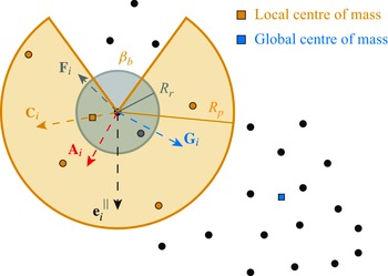
A schematic of a SPP $i$ and its neighbourhood. The tendency to maintain is previous direction vector $\mathbf {e}_{i, t}^{\|}$ , the attraction to the global centre of mass ${\mathbf {G}}_{i, t}$ and the noise vector $\hat {\boldsymbol {\epsilon }}_{i, t}$ are independent of the local neighbourhood. The particle $i$ interacts with its neighbours within a distance $R_p$ through local attraction $\hat {\mathbf {C}}$ and alignment $\hat {\mathbf {A}}_{i, t}$ , except for the blind zone specified by $\beta _b$ of the focal particle $i$ . The particle $i$ experiences a repulsive force $ \mathbf {F}_{i, t}$ by its neighbours with a distance less than $R_r$ . Note that there is no blind zone for the repulsion.

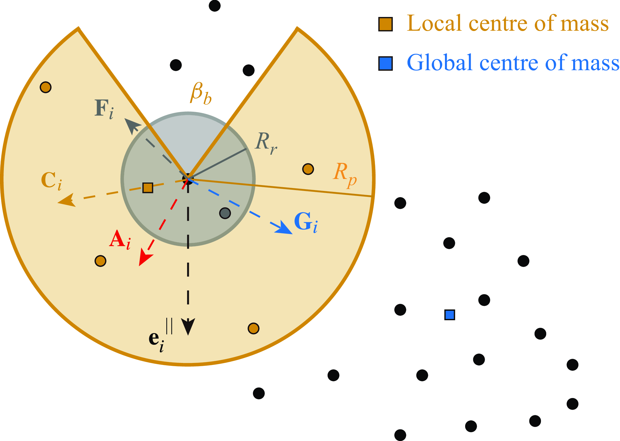
As reviewed in the introduction, the main differences between different agent-based models lie in how the neighbours of a focal agent are determined, and the social forces involved in the local interaction rule. We build the agent-based model upon the previous studies (Strömbom Reference Strömbom2011; Strömbom et al. Reference Strömbom, Siljestam, Park and Sumpter2015). The swimming trajectories of individuals within a fish group are modelled by SPPs. Each fish is represented as an identical particle moving in a cyclic two-dimensional space of dimensions $L \times L$ . An individual interacts with others through social forces within a metric neighbourhood, defined by a certain distance, as illustrated in figure 1. Each particle’s perceptual field encompasses a zone with a radius of $R_p$ centred on it. To account for the fish’s blind spot, this perceptual field omits a sector characterised by a blind angle $\beta _b$ . The local repulsion term is influenced by all particles within a proximity of $R_r$ , without any exclusion due to blind zones.

The initial positions of these individuals are generated using uniformly distributed random numbers within the interval $ [ {0,L} ]$ , while their initial orientations are randomised within $ [ { - \pi ,\pi } ]$ . The equation governing translational motion is formulated as

(2.1)

\begin{equation} \mathbf {r}_{i, t+1}=\mathbf {r}_{i, t}+v \Delta t \cdot \dot {\mathbf {r}}_{i, t}, \end{equation}

where $\mathbf {r}_{i, t}= [x_{i, t}, y_{i, t} ]^{\mathbf {T}}$ denotes the position vector of the $i$ th individual at the time $t$ , $v$ signifies the individual’s speed and $\dot {\mathbf {r}}_{i,t}$ represents the directional vector

(2.2)

\begin{equation} \dot {\mathbf {r}}_{i, t}=\mathbf {e}_{i, t}^{\|}=\left [{e}_{i, t, x}^{\|}, {e}_{i, t, y}^{\|}\right ]^{\mathbf {T}}. \end{equation}

Note that $\mathbf {e}_{i, t}^{\|}$ is a unit vector, with its evolution described by

(2.3)

\begin{equation} \mathbf {e}_{i, t+1}^{\|}=\frac {d \mathbf {e}_{i, t}^{\|}+(c \hat {\mathbf {C}}_{i, t}+a \hat {\mathbf {A}}_{i, t}+r \mathbf {F}_{i, t}+g {\mathbf {G}}_{i, t}+e \hat {\boldsymbol {\epsilon }}_{i, t})\Delta t}{\left |d \mathbf {e}_{i, t}^{\|}+(c \hat {\mathbf {C}}_{i, t}+a \hat {\mathbf {A}}_{i, t}+r \mathbf {F}_{i, t}+g {\mathbf {G}}_{i, t}+e \hat {\boldsymbol {\epsilon }}_{i, t})\Delta t\right |}. \end{equation}

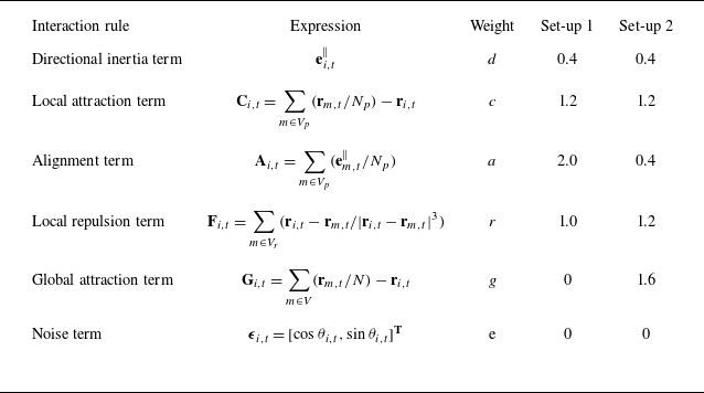
The terms in (2.3) are as follows. The directional inertial term $\mathbf {e}_{i, t}^{\|}$ signifies the individual’s tendency to maintain its direction from the previous time step. The local attraction term $\hat {\mathbf {C}}_{i, t}$ represents the unit vector pointing from the $i$ th individual’s current position to the local centre of mass, calculated as the centroid of all neighbours within the individual’s perceptual field. The local alignment term $\hat {\mathbf {A}}_{i, t}$ aligns with the average motion direction of all neighbours within the individual’s perceptual field. The local repulsion term $\mathbf {F}_{i, t}$ accounts for the individual’s tendency to avoid close neighbours within the repulsion zone. The global attraction term ${\mathbf {G}}_{i, t}$ directs the individual towards the global centroid from its current position. The term $\hat {\boldsymbol {\epsilon }}_{i, t}$ introduces randomness conforming to a standard normal distribution. To each of the vectors, we attach a corresponding weight $d$ , $c$ , $a$ , $r$ , $g$ and $e$ , specifying the relative strength of each term. The symbol $\hat {\,}$ denotes unit vectors, normalised by their original magnitudes, with the expressions summarised in table 1. Note that only ${\mathbf {G}}_{i, t}$ and $\mathbf {F}_{i, t}$ are not normalised, so attraction to the global centre of mass increases with distance and the repulsive force becomes significantly large when two individuals approach each other.

Table 1.

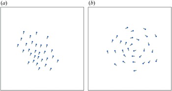
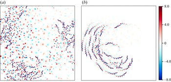
The expressions for different terms in (2.3), representing different interaction rules. Here, $i$ represents the focal individual and $m$ represents its neighbour; $V_p$ and $V_r$ denote the perceptual and repulsive zones, as illustrated respectively by orange and grey colours in figure 1; and $V$ represents the entire computational domain. The simulated results for two typical set-ups, 1 and 2, are plotted in figure 2.

Figure 2.

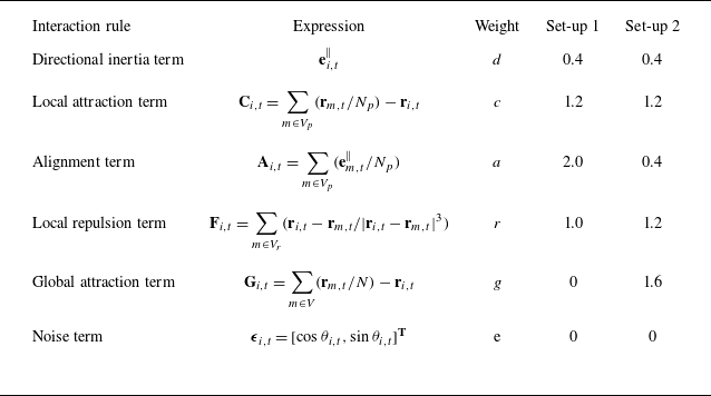
Plots of the instantaneous swimmer positions for two different numerical set-ups of the SPP model (as listed in table 1) representing two distinct collective patterns: ( $a$ ) schooling for set-up 1 and ( $b$ ) milling for set-up 2. Both cases consider 20 individuals.

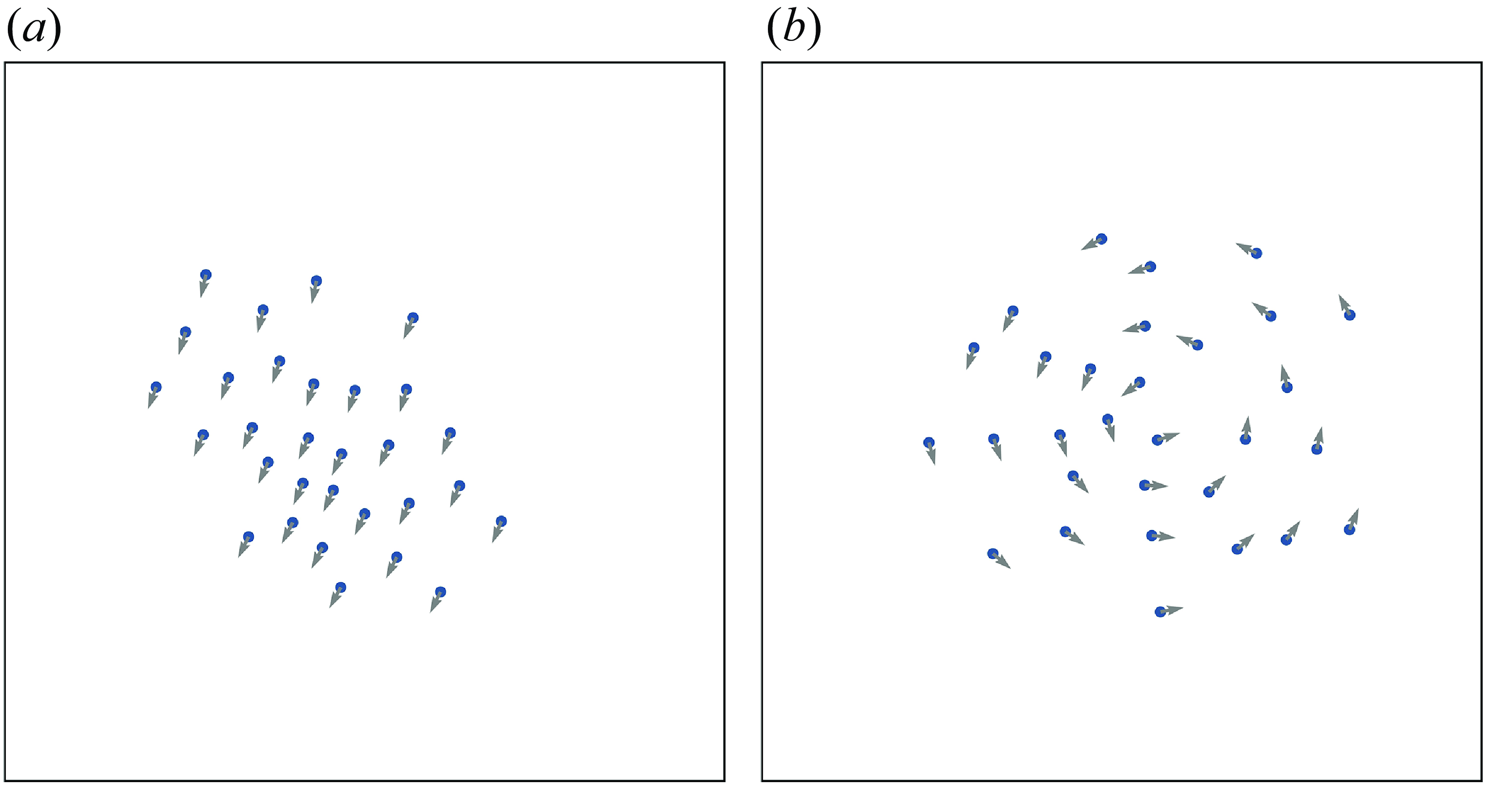
Here, based on the values of the parameters, collective motion can emerge in different modes. As the parameter $a$ increases, the phase ‘schooling’ will emerge, as shown in figure 2( $a$ ), exhibiting a highly coordinated collective motion. The phase ‘milling’, which forms a ‘vortex’ with each individual following an approximately circular trajectory, is shown in figure 2( $b$ ). In order to achieve a more stable milling phase, we make some modifications in the global attraction term of (2.3). In the interaction rule for each individual, $\mathbf {G}_{i, t}$ is cross-multiplied with a unit vector in the $z$ -direction so that each individual gets a tendency to rotate around the global centroid.

2.2. Computational fluid dynamics model

The flow environment around the fish is governed by the two-dimensional viscous incompressible NS equations, as given by

(2.4)

\begin{equation} \rho \left ( {\frac {{\partial {\textbf {u}}}}{{\partial t}} + {\textbf {u}} \cdot \nabla {\textbf {u}}} \right ) = - \nabla p + \mu {\nabla ^2}{\textbf {u}} + {\textbf {f}}, \end{equation}

(2.5)

\begin{equation} \nabla \cdot {\textbf {u}} = 0, \end{equation}

where $\rho$ denotes the fluid density, $\textbf {u}$ represents the flow velocity, $p$ signifies the fluid pressure, $\mu$ is the constant dynamic viscosity of the fluid and $\textbf {f}$ represents the force exerted on the fluid by the immersed boundary. This additional forcing term $\textbf {f}$ is determined by integrating the Lagrangian forcing density $\mathbf {F}(s, t)$ , as expressed by

(2.6)

\begin{equation} \mathbf {f}(\mathbf {x}, t)=\int \mathbf {F}(s, t) \delta (\mathbf {x}-\mathbf {X}(s, t)) {\rm d}s, \end{equation}

where $\delta$ denotes the Dirac-delta function, which we replace with a smooth function $\delta _h$ for computational purposes. The fluid and structural coordinates are denoted by $\mathbf {x}$ and $\mathbf {X}$ , respectively. The expression for the smooth function $\delta _h$ is

(2.7)

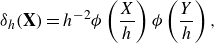\begin{equation} \delta _h(\mathbf {X})=h^{-2} \phi \left (\frac {X}{h}\right ) \phi \left (\frac {Y}{h}\right ), \end{equation}

where $h$ is the length of the computational cell, $X$ and $Y$ signify the position within the computational cell. The function $\phi$ is defined as

(2.8)

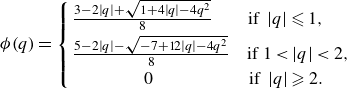\begin{equation} \phi (q) = \left \{ \begin{array}{l} \frac {{3 - 2|q| + \sqrt {1 + 4|q| - 4{q^2}} }}{8}{\rm {\quad \quad if}}\ \left | q \right | \leqslant 1 ,\\[3pt] \frac {{5 - 2|q| - \sqrt { - 7 + 12|q| - 4{q^2}} }}{8}{\rm {\quad if\ 1}}\lt \left |q\right |\lt 2 ,\\[3pt] \qquad \qquad 0{\rm {\;\;\qquad \qquad \quad if\ }} \left | q \right | \geqslant 2. \end{array} \right . \end{equation}

In (2.6), the Lagrangian forcing density, denoted as $\mathbf {F}(s, t)$ , is expressed as

(2.9)

\begin{equation} \mathbf {F}=\alpha _F \int _0^t\left (\mathbf {U}_{i b}-\mathbf {U}\right ) \mathrm {d} t^{\prime }+\beta _F\left (\mathbf {U}_{i b}-\mathbf {U}\right ), \end{equation}

where $\mathbf {U}_{i b}$ represents the interpolated fluid velocity on the immersed boundary, while $\mathbf {U}$ denotes its targeted moving velocity and $\alpha _F$ and $\beta _F$ are two large, negative constants (Goldstein, Handler & Sirovich Reference Goldstein, Handler and Sirovich1993; Li et al. Reference Li, Liu, Deng, Lutz and Xie2021a ; Liu et al. Reference Liu, Wang, Mao and Deng2023b ).

To reduce the computational cost, we represent the fish body as a one-dimensional filament with a non-uniform density distribution. The density distribution is based on a simplified physical model of zebrafish, expressed as

(2.10)

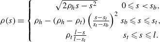\begin{equation} \rho (s)=\left \{\begin{array}{cc} \sqrt {2 \rho _h s-s^2} & 0 \leqslant s\lt s_b ,\\ \rho _h-\left (\rho _h-\rho _t\right )\left (\frac {s-s_t}{s_t-s_b}\right )^2 & s_b \leqslant s \leqslant s_t, \\[5pt]\rho _t \frac {l-s}{l-s_t} & s_t \leqslant s \leqslant l. \end{array}\right . \end{equation}

where $s$ is the Lagrange coordinate in the satellite coordinate system distributed along the centre line of the fish, $l$ is the length of the fish. Other parameters are set accordingly, $\rho _h=s_h=0.04 l$ , $s_t=0.95 l$ , $\rho _t=0.01 l$ . We note that the fish is segmented at the same length scale as the surrounding Eulerian mesh. Therefore, an increase in the number of Lagrangian points on the fish results in a proportional increase in the number of Eulerian mesh cells within the computational domain (Deng, Mao & Xie Reference Deng, Mao and Xie2019).

The fish’s kinematic deformation is given by

(2.11)

\begin{equation} \zeta (s,t) = A(t)\sigma (s)\tau (t) \cdot \sin (2\pi s + \beta (t) + \phi ), \end{equation}

where $\zeta (s,t)$ represents the lateral displacement of the fish’s mid-line in the local coordinate system. Here, $A(t)$ is the motion amplitude of the fish wave equation. The function $\sigma (s)$ has been set $\sigma (s)= s$ , represents the amplitude of the travelling wave as linear amplification from the head to the tail. The function $\tau (t)$ is a starting function, which allows the travelling curvature wave to be applied gradually. Here, $\tau (t)$ is defined as

(2.12)

\begin{equation} \tau (t)=\left \{\begin{array}{cc} \frac {t}{T_s}-\frac {1}{2 \pi } \sin \left (\frac {2 \pi t}{T_s}\right ) & 0 \leqslant t \leqslant T_s, \\ 1.0 & t\gt T_s ,\end{array}\right . \end{equation}

where $T_s$ is the time needed for the startup phase.

We accomplish small turning action in the fish’s body by introducing a compensation function

(2.13)

\begin{equation} Q(s, t)=B(t) \tau (t) s^p, \end{equation}

where $B$ is a coefficient, its magnitude and sign respectively represent the degree and direction of the small turning action. The exponent $p$ modifies the distribution of the compensation function along the fish’s body, with $p = 2$ in this instance. The compensation function is superimposed onto the base fish wave by adding curvature, as follows:

(2.14)

\begin{equation} k(s, t)=k_{{base }}(s, t)+k_{ {turn }}(s, t), \end{equation}

where ${k_{base}}(s,t)$ is the curvature along the mid-line of the fish, which travels from the head to the tail as a wave, and ${k_{turn}}(s,t)$ represents the curvature of turning motion.

In (2.11), the function $\beta (t)$ represents the frequency of tail beat, which is regulated by a central pattern generator (CPG) controller, expressed as

(2.15)

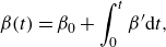\begin{equation} \beta (t)=\beta _0+\int _0^t \beta ^{\prime } {\rm d}t, \end{equation}

where the time-varying component $\beta ^{\prime }(t)$ is defined by the integral

(2.16)

\begin{equation} \beta ^{\prime }(t)=\int _0^t -\alpha _\omega \left (\beta ^{\prime }-2 \pi \omega _{t a r}\right ) {\rm d} t. \end{equation}

Here, $\omega _{t a r}$ is the target frequency. The transition rate from the tail beat’s current frequency to its target value is represented by the coefficient $\alpha _\omega$ , and we set $\alpha _\omega =4$ . Our previous study (Liu et al. Reference Liu, Wang, Mao and Deng2023b ) has shown that this parameter choice can achieve a satisfactory control performance. By altering the frequency of its body wave, we are able to modify the fish’s speed.

We establish two coordinate systems to describe the motion of fish in the flow field. A spatial coordinate system is used to describe the translational and rotational motion of the fish body. Additionally, for each fish, a body-fixed coordinate system is established with the head of the fish as the reference point ( $O_c$ ). This body-fixed coordinate system is utilised to describe the variations in individual fish body waves. The motion of the body-fixed coordinate system is described by the forces and torques exerted by the fluid on the fish’s body. These forces and torques are obtained by integrating along the fish’s body, as follows:

(2.17)

\begin{equation} m \ddot {\mathbf {x}}_c=\mathbf {F}_c ,\end{equation}

and

(2.18)

\begin{equation} I_z \ddot {\theta }_c=M_z, \end{equation}

where $m$ is the mass of the fish, $I_z$ represents the moment of inertia about the z-axis, $\ddot {\mathbf {x}}_c$ denotes the acceleration of the reference point $O_c$ , $\ddot {\theta }_c$ is the angular acceleration of the body-fixed coordinate system and $\mathbf {F}_c$ and $M_z$ characterise the forces and moments exerted by the fluid on the individual. Here, $\mathbf {F}_c$ , $M_z$ and $I_z$ are calculated as follows:

(2.19)

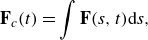\begin{equation} \mathbf {F}_c(t)=\int \mathbf {F}(s, t) \mathrm {d} s, \end{equation}

(2.20)

\begin{equation} M_z(t)=\int \left (\mathbf {r}_c \times \mathbf {F}(s,t)\right ) \cdot \mathbf {e}_z \mathrm {d} s ,\end{equation}

and

(2.21)

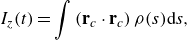\begin{equation} I_z(t)=\int \left (\mathbf {r}_c \cdot \mathbf {r}_c\right ) \rho (s) \mathrm {d} s, \end{equation}

where $\mathbf {r}_c$ denotes the position vector from $O_c$ to a discrete point on the fish’s body, and $\mathbf {e}_z$ stands for the unit vector along the z-axis.

2.3. Hybrid model for collective motion

Figure 3.

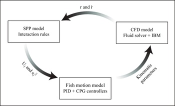
Schematic illustration of the hybrid model, which couples the SPP model and the CFD model through a CPG controller.

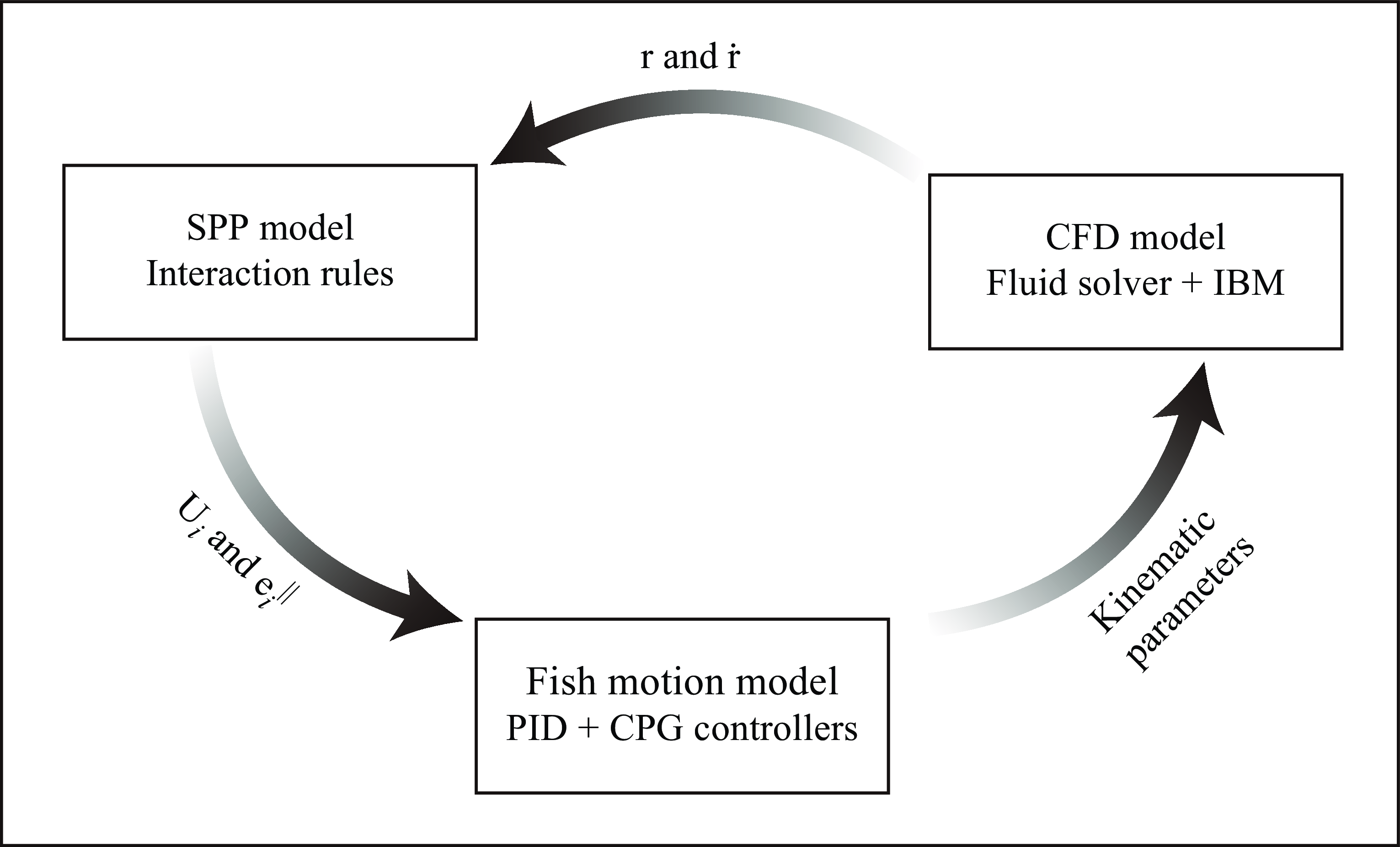
The SPP model is an efficient method for simulating the movement of large-scale swarms. However, it simplifies individual motion processes, neglecting the interactions between swimmers and the fluid environment. Hydrodynamic effects, which have a significant impact on simulating the swimming of fish schools, are overlooked in this model. To couple behavioural rules with hydrodynamic interactions, we propose combining the SPP model with CFD simulation, as shown in figure 3.

The SPP model calculates the target direction for each individual based on its current position and direction, following the interaction rules. In other words, the SPP model determines whether individuals in the group need to turn and alter their speed. In the fish motion model, each individual adjusts its undulating pattern based on the results computed by the SPP model. For CFD calculations, the motion of each individual is actively exerted by the body waves output from the fish motion model. The immersed boundary method (IBM) method is applied to calculate the forces on the fish body, which is simplified into a thin filament, in the current flow field. The position and direction of each individual in the spatial coordinate system are updated with the forces and moments exerted by the fluid. The new flow field information is obtained by solving the NS equations. The individual position and motion direction are then re-calculated as input information to the SPP model. The three models cycle through the computation to realise the numerical simulation of coordinated swimming considering hydrodynamic effects.

We note that constraints on both the swimming speeds and the turning rates of the individuals should be introduced to fit the current hybrid model for two reasons. First, both the undulating frequency and amplitude of the fish tail are limited, resulting in a maximum swimming speed and a peak value of acceleration (manoeuvrability). The same applies to the rotational angular velocity or turning rate. Second, for the fish body with a finite length considered in our CFD model, it occupies a certain spatial position. Differentiating from previous SPP models, which typically consider volumeless particles, overlap or collisions between individuals in our hybrid model should be avoided.

Figure 4.

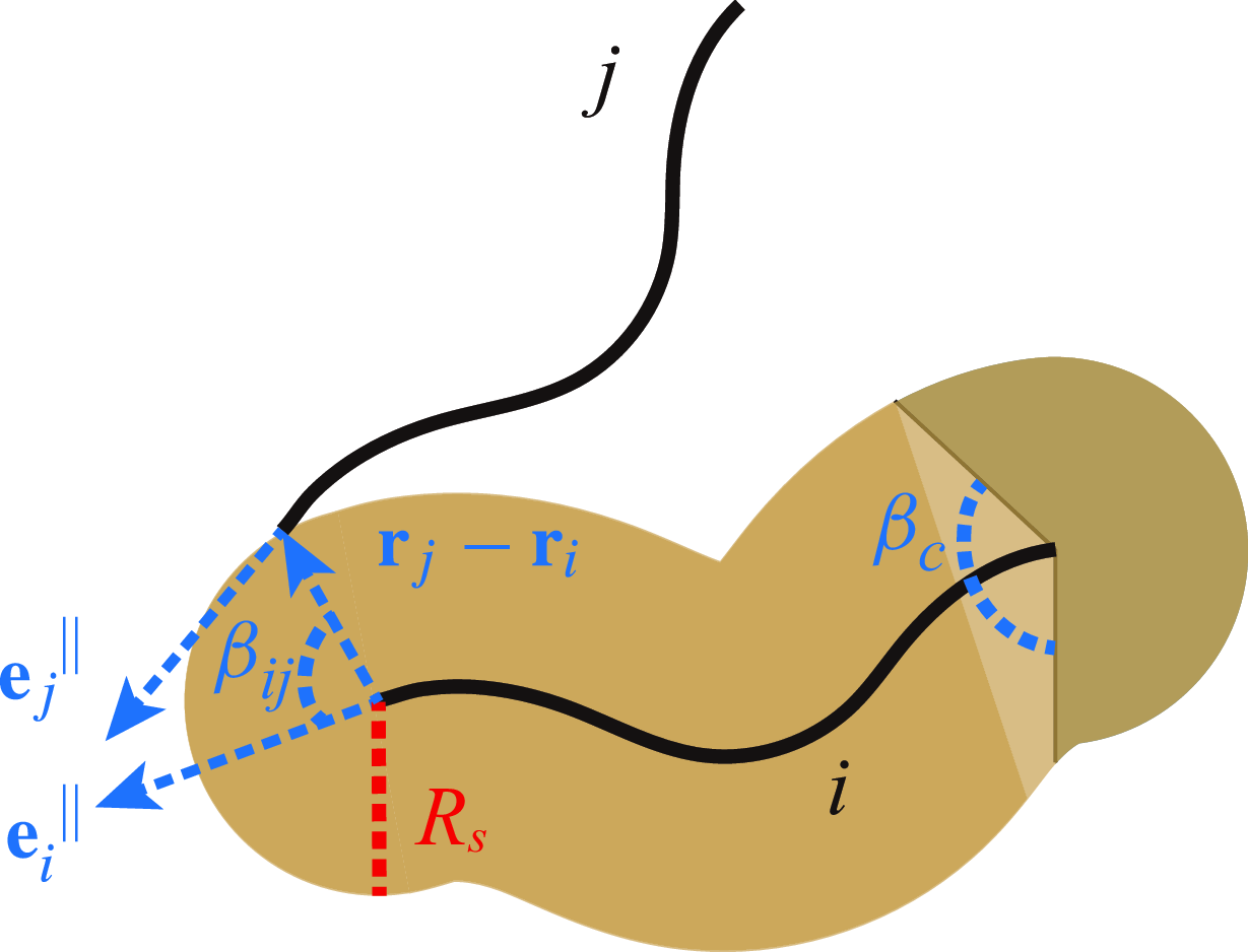
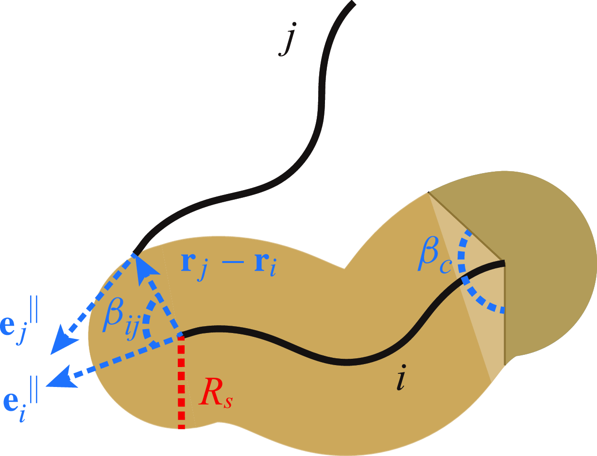
Illustration of the buffer zone for collision avoidance when two fish approach too closely to each other. Here, $\mathbf {e}_{i}$ represents the directional vector of the currently considered fish, and $\mathbf {e}_{j}$ represents the directional vector of its neighbour. The vector $\mathbf {r}_{j}-\mathbf {r}_{i}$ is the distance vector of the two fish heads. The angle $\beta _{ij}$ is the intersection angle between $\mathbf {e}_{i}$ and $\mathbf {r}_{i}$ , and $\beta _{c}$ is a critical angle, and we set $\beta _{c} = \beta _{b}$ .

We first set an initial target speed $U_{tar}$ for the SPP individuals, which can be achieved by a single freely swimming fish in the CFD simulations with a certain combination of undulating frequency and amplitude. However, as two fish approach too closely to each other, expecting them to collide or overlap, we introduce a collision avoidance mechanism by decelerating one of these two fish.

We define a buffer zone for the currently considered fish $i$ , as shown in figure 4. One filament represents one fish body, with a distance $R_s$ from the body determining the range of buffer zone. When fish $j$ enters the buffer zone of fish $i$ , and the swimming direction of fish $j$ meets certain requirements, fish $i$ decelerates to a new speed $U_i$ according to a speed ratio $\gamma _i$ , ranging between 0 and 1. Here, $\gamma _i$ is calculated as

(2.22)

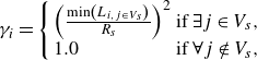\begin{equation} {\gamma _i} = \left \{ {\begin{array}{*{20}{l}} {{{\left ( {\frac {{\min \left ( {{L_{i,j \in {V_s}}}} \right )}}{{{R_s}}}} \right )}^2}}&{{\rm { if }}\,\exists j \in {V_s}},\\ {1.0}&{{\rm { if }}\,\forall j \notin {V_s}}, \end{array}} \right . \end{equation}

where $L_{i,j}$ represents the minimum distance between fishes $i$ and $j$ , and $V_s$ denotes the fish $i$ buffer zone. After all its neighbours have left the buffer zone, its speed recovers to the initial target speed $U_{tar}$ . We note that the value of $R_s$ for fish $i$ depends on its mean speed (averaged in the last undulating cycle), given by $R_s=R_0 \overline{U_i}/U_{tar}$ ( $R_0 = 0.5l$ ). It is easy to understand that a fish with a faster swimming speed should have a larger buffer zone for effective collision avoidance.

The criteria for initiating obstacle avoidance strategy are illustrated in figure 4. First, at least one neighbour, for example fish $j$ , enters the buffer zone of fish $i$ . We note that fish $i$ tends to get close to fish $j$ in the current swimming direction only when the angle between $\mathbf {r}_j - \mathbf {r}_i$ (relative position vector) and $\mathbf {e}_i^{\|}$ (swimming direction of individual $i$ ) is less than $\beta _c/2$ , where $\beta _c$ is the perception angle of fish $i$ . In that case, fish $i$ will decelerate to avoid colliding with fish $j$ . Additionally, if more than one individuals enters the buffer zone of fish $i$ , its nearest neighbour will be chosen for obstacle avoidance determination, as implied in (2.22).

Subsequently, the new positions for individuals in the modified SPP model will be updated by

(2.23)

\begin{equation} \mathbf {r}_{i, t+1}=\mathbf {r}_{i, t}+U_{tar} \gamma _i \Delta t \cdot \dot {\mathbf {r}}_{i, t}. \end{equation}

Moreover, the turning rate or angular speed of the fish should also be constrained because the turning rate calculated from the SPP model cannot always be successfully achieved by the CFD model, akin to the turning manoeuvrability of a real fish. We define a maximum angular speed $\omega _{\textit{max}}$ through testing our CFD model. Further, the angular speed should also be related to the forward swimming speed, as a faster swimming fish can gain a higher turning ability. Using the speed ratio $\gamma _i$ , we limit the maximum angular speed of fish $i$ as

(2.24)

\begin{equation} \omega _{m,t}=\gamma _i \omega _{\textit{max}}, \end{equation}

and we modify the target angular speed of fish $i$ to

(2.25)

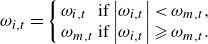\begin{equation} {\omega _{i,t}} = \left \{ {\begin{array}{*{20}{l}} {{\omega _{i,t}}}&{{\rm { if }}\left | {{\omega _{i,t}}} \right | \lt {\omega _{m,t}}},\\ {{\omega _{m,t}}}&{{\rm { if }}\left | {{\omega _{i,t}}} \right | \geqslant {\omega _{m,t}}} .\end{array}} \right . \end{equation}

After receiving the target swimming speed $U_i$ and angular speed $\omega _{i,t}$ , the fish motion model, illustrated in figure 3, determines a set of kinematic parameters for the fish’s undulating motion to achieve these targets. This is realised using a proportional–integral–derivative (PID) controller, which we have adopted in our previous study (Liu et al. Reference Liu, Wang, Mao and Deng2023b ). It is important to note that a CPG controller is implemented to output rhythmic signals based on the target’s frequency and phase, as introduced in § 2.2. This allows the fish body wave to smoothly transition between different frequencies and phases without explicitly relying on time terms for calculation (Li et al. Reference Li, Liu, Deng, Lutz and Xie2021a ).

Unless otherwise specified, all quantities in the current study have been non-dimensionalised. To correlate with a natural fish group, for example, the Rummy-nose tetra (with an average body length of 5 cm) used in a laboratory-scale water tank (Lafoux et al. Reference Lafoux, Moscatelli, Godoy-Diana and Thiria2023), a unit length corresponds to 5 cm, a unit time corresponds to 0.5 s and a unit speed corresponds to 10 cm s⁻¹ (or 2 body lengths per second). Note that the swimming speed of 2 body lengths is lower than the widely reported cruise speed for small fish, though it remains within a reasonable range for fish groups swimming freely in still water (Sánchez-Rodríguez et al. Reference Sánchez-Rodríguez, Raufaste and Argentina2023). By setting the fluid viscosity appropriately, the swimming locomotion leads to Reynolds numbers around 500 based on the undulating amplitudes.

2.4. Basic function tests on a minimal group

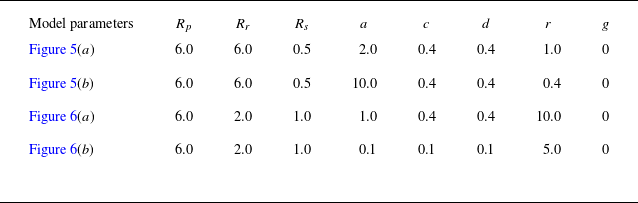
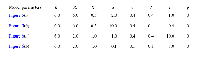
Before simulating large-scale collective behaviour, it is essential to validate the basic functions of the interaction rules in the model. This section focuses specifically on the alignment term and the local repulsion term, by tuning their respective weights, $a$ and $r$ , as outlined in table 2, using a minimal group of two individuals.

Table 2.

Model parameters used in the basic function tests, corresponding to the simulated results shown in figures 5 and 6. Note that $R_p$ and $R_r$ are illustrated in figure 1; $R_s$ is illustrated in figure 4; and $a$ , $c$ , $d$ , $r$ and $g$ are the SPP model weights, as listed in table 1.

Figure 5.

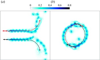
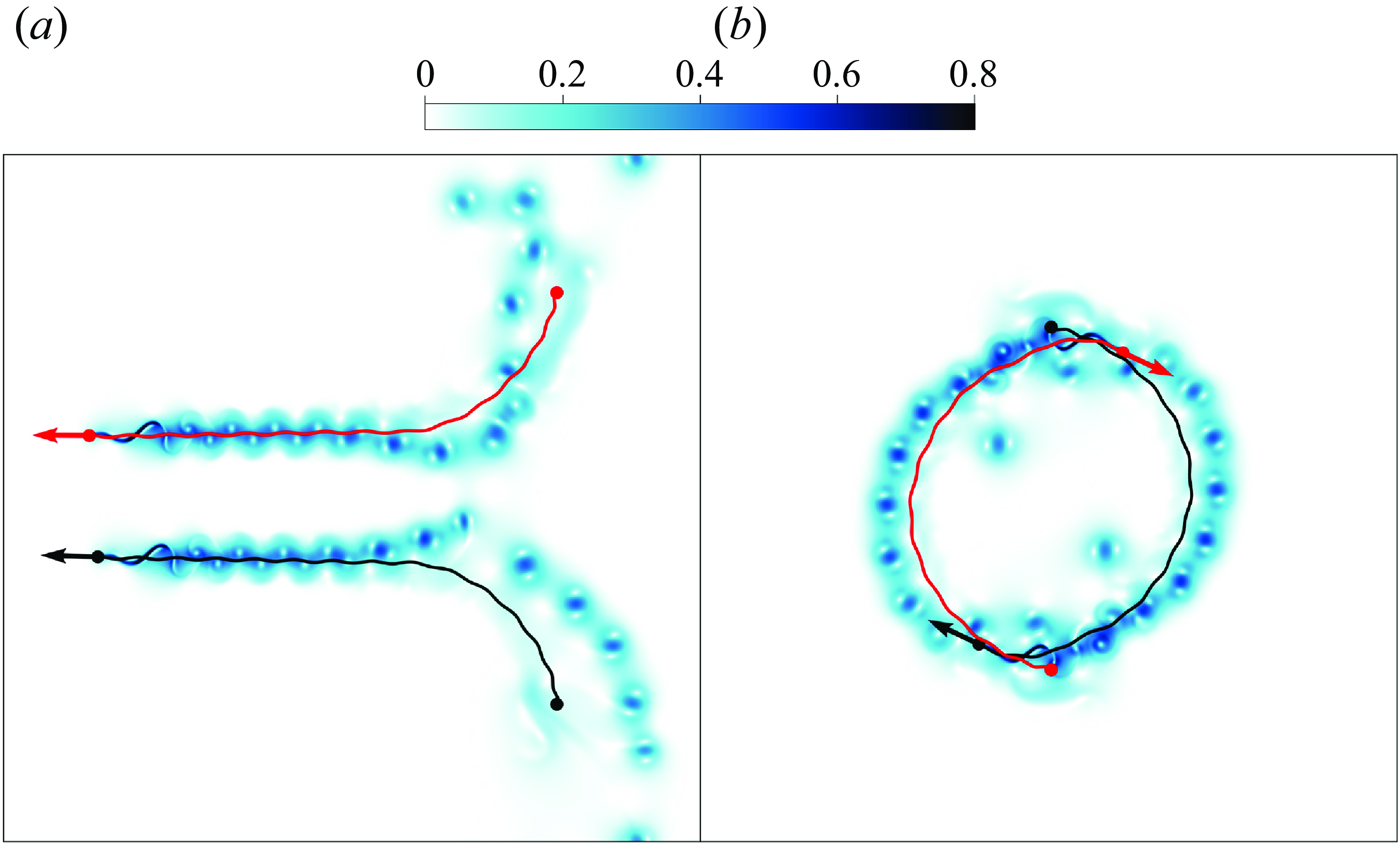
Basic functionality test of the hybrid model with a minimal group of two fish. ( $a$ ) Depicts an approach followed by side-by-side swimming, while ( $b$ ) illustrates mutual orbiting behaviour. Swimming trajectories are shown as lines in different colours (red and black) for the two individuals. The dots without arrows indicate the starting positions, and arrows represent the instantaneous swimming directions. The flow fields are coloured by the velocity magnitude, with a gradient from light blue (low velocity) to dark blue (high velocity). Model parameters are listed in table 2.

Figure 6.

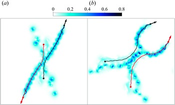
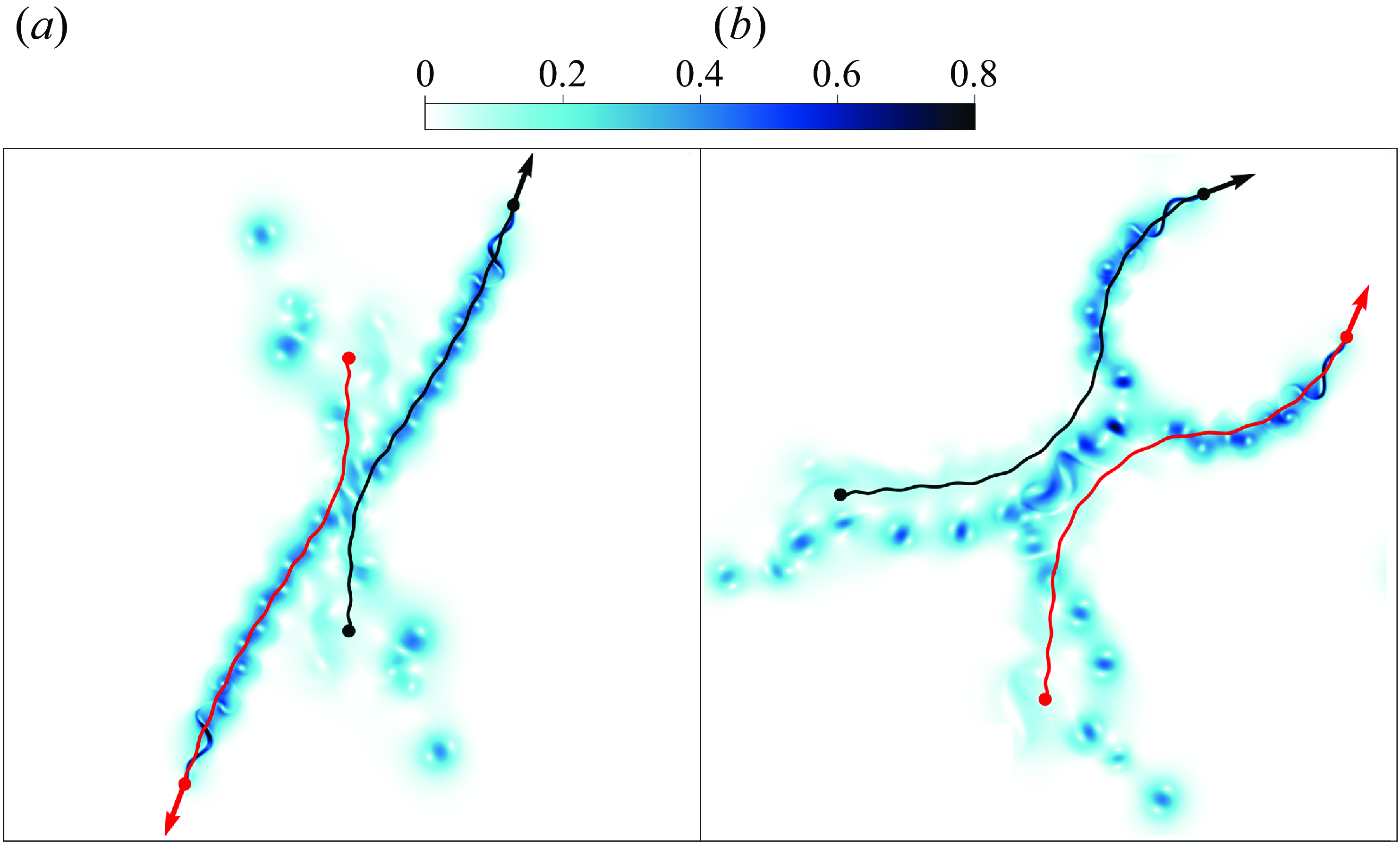
Basic functionality test of the hybrid model with a minimal group of two fish. ( $a$ ) Shows an approach followed by staggered departure, while ( $b$ ) shows an approach follow by departure at a certain distance. Swimming trajectories are shown as lines in different colours (red and black) for the two individuals. The dots without arrows indicate the starting positions, and arrows represent the instantaneous swimming directions. The flow fields are coloured by the velocity magnitude, with a gradient from light blue (low velocity) to dark blue (high velocity). Model parameters are listed in table 2.

To test the effect of the alignment term in the hybrid model, the coefficient of the alignment term $a$ is set according to the values in table 2, while the strengths of the other terms (i.e. $c$ , $d$ , $r$ and $g$ ) are relatively reduced. The results are shown in figure 5, where the trajectories of the two individuals are marked with black and red solid lines, the arrows represent the swimming directions and the coloured fields denote the velocity magnitude of the flow. In figure 5( $a$ ), when two fish swim in opposite directions, as they approach a distance less than $R_p$ , their directions of motion gradually converge under the influence of the alignment term. Through small turning movements, the two fish end up swimming side by side in the same direction. In figure 5( $b$ ), when two fish are initially within the range of the alignment term’s influence, with strictly opposite directions and no other factors interfering, a special motion pattern is observed. The two individuals rotate around their centre while keeping their directions of motion opposite at all times, and this rotational motion continues until an external disturbance occurs. This behaviour stems from the interplay of various interaction terms: the alignment term acts in the opposite direction to the individuals’ current velocity vectors, while the local attraction and repulsion terms exert forces perpendicular to the direction of motion. Notably, the local attraction term exerts a predominant influence due to the spatial separation between the individuals. Ultimately, for each individual, only the action along the direction of motion and the action pointing towards the local centre of mass (the midpoint between the two individuals) are affected. This causes the two individuals to rotate around the local centre of mass until disturbed by an external factor. As the number of individuals increases, this particular pattern ceases to occur, thereby having no impact on collective motion simulation.

To evaluate the impact of the local repulsion term within the model, we increase the weight $r$ while decreasing the coefficients associated with other interaction terms. The simulation outcomes for two fish, predominantly influenced by the local attraction term, are presented in figure 6. In figure 6( $a$ ), when two fish are swimming in opposite directions, the local repulsion term alters their swimming direction, causing them to stagger as they gradually approach each other. Figure 6( $b$ ) illustrates the collision avoidance process between two individuals whose initial swimming directions intersect, influenced by the repulsive force term. When the distance between them becomes too close, the two individuals simultaneously execute a turning action to prevent collision. Once a sufficient distance is established between them, they move side by side under the influence of the alignment term. The trajectories of the two individuals remain essentially symmetrical throughout the process.

3. Sensitivity study and verification of the numerical models

Before presenting the results from the newly developed hybrid model, we conduct sensitivity tests on the individual components of the simulation: the agent-based SPP model and the CFD model.

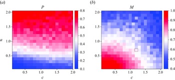
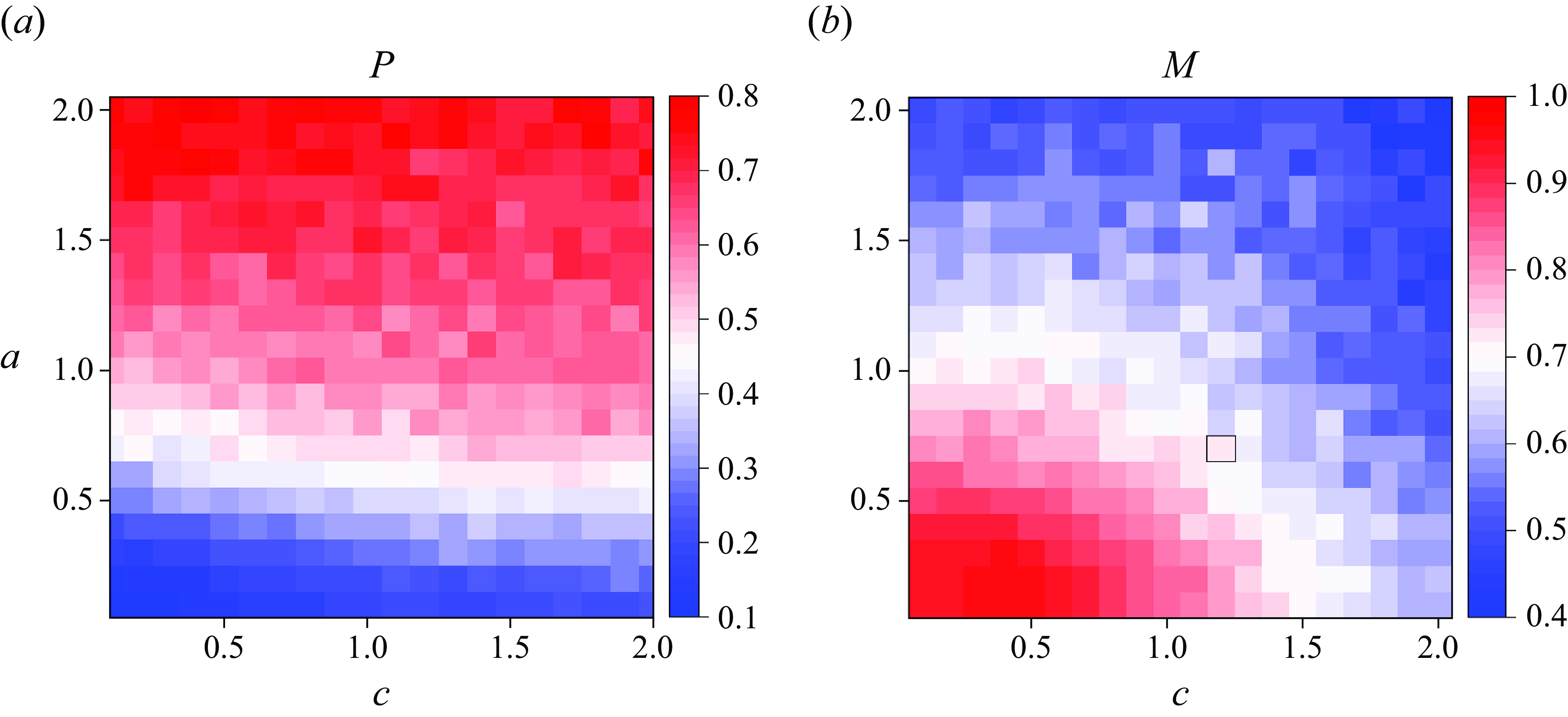
We begin by performing a sensitivity analysis on the interaction rule parameters of the SPP model. Given the large number of parameters involved, a comprehensive examination across the entire parametric space would be computationally prohibitive. Therefore, we restrict the study to a subspace spanned by two representative parameters: the local alignment term, $a$ , and the local attraction term, $c$ . In this analysis, we fix the directional inertial term at $d=0.4$ , the local repulsion at $r=1.2$ , and the global attraction term at $g=0.5$ . Figure 7 presents contour plots of the order parameter $P$ , which quantifies the schooling behaviour, and the milling parameter $M$ , which characterises milling patterns, as functions of $a$ and $c$ . From the results, it is evident that the schooling pattern, as indicated by $P$ , is highly sensitive to the variation of $a$ and exhibits only weak dependence on $c$ (figure 7 $a$ ). Specifically, an increase in $a$ leads to a transition to a more highly coordinated schooling pattern. In contrast, the milling pattern, represented by $M$ , is influenced by both $a$ and $c$ (figure 7 $b$ ). For lower values of both $a$ and $c$ , a distinct milling pattern emerges, which gradually diminishes as either or both of these parameters increase.

Figure 7.

Contour plots of the order parameter $P$ and the milling parameter $M$ within the parametric space defined by the parameters $a$ and $c$ : ( $a$ ) $P$ increases with the rise in $a$ , marking the phase transition to a highly coordinated schooling pattern; ( $b$ ) $M$ identifies a milling pattern in the bottom-left corner, where both the local alignment term and local attraction terms are at low intensities. For each pair of parameters $a$ and $c$ , 50 simulation runs are conducted with varying random initialisation over 8 000 time units, with the last 1 000 time units used to calculate the average values of $P$ and $M$ .

Figure 8.

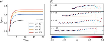
Simulation results for an uncontrolled fish swimming with varying mesh resolutions: ( $a$ ) swimming speed and ( $b$ ) vorticity contours.

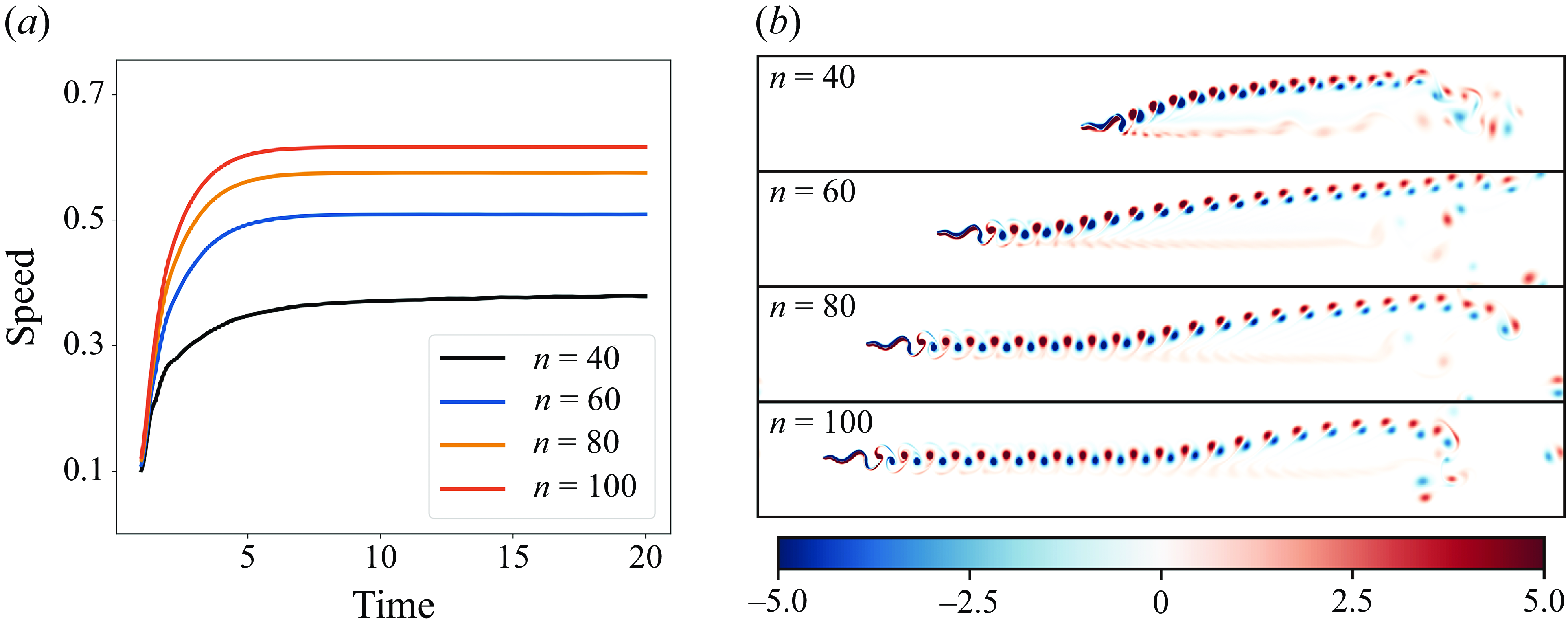
Next, we evaluate the spatial accuracy of the CFD model by conducting a sensitivity analysis on the grid resolution, using freely swimming fish as the test case. We vary the number of Lagrangian points, $n$ , on the fish, and examine four different spatial resolutions: $n=40$ (with 640 000 cells), $n=60$ (with 1 440 000 cells), $n=80$ (with 2 560 000 cells) and $n=100$ (with 4 000 000 cells). Figure 8( $a$ ) exhibits the swimming speed of the fish over 20 undulation cycles for each resolution. The results indicate that the mesh with $n=80$ provides sufficient spatial accuracy, with a discrepancy of only 6.6 % in the steady swimming speed compared with the results of $n=100$ . In figure 8( $b$ ), the vorticity contours generated by the swimmer are shown for each mesh resolution. The wake patterns and vortex structures are consistent between $n=80$ and $n=100$ , with no observable differences. Compromising between computational cost and efficiency, the mesh with $n=80$ is selected as the optimal spatial resolution for the subsequent simulations.

4. Results and discussion

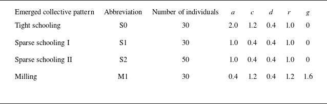
To demonstrate the capabilities of our hybrid model, we conduct numerical simulations of both schooling and milling behaviours in large fish groups. The computational domain is set to a size of $20l \times 20l$ with periodic boundary conditions, where $l$ is the length of an individual fish. We achieve specific formations and group compactness by mainly varying the parameters of the SPP model in (2.3). Four distinct collective modes are considered, with parameters listed in table 3. For each individual in the four groups, we set the perceptual field radius to $R_p = 6l$ , the local repulsion radius to $R_r = 6l$ and the blind angle to $\beta _b = 0.5\pi$ . In the SPP model, the position of each particle corresponds to the location of the fish head. For fish kinematics, the initial undulation amplitude is set at $0.2l$ , and the undulatory frequency is set at $1$ (please note the parameter non-dimensionalisation introduced above). For convenience, we denote this initial undulatory period as $T$ . Within our hybrid model, individual swimming speeds are adjusted by modifying the undulatory frequency while maintaining a constant amplitude. It is important to note that the initial undulatory frequency serves as the upper limit for fish motion. In situations where collision avoidance is necessary, the involved fish would first decrease its frequency to reduce speed, and then return to the initial frequency after steering clear of potential collisions.

Table 3.

The parameters set for four simulation cases. The parameters are derived from (2.3). For more details, please refer to table 1.

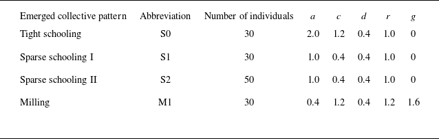
It is well established that fish in groups exhibit significant differences in swimming speed and power expenditure compared with solitary fish (Ligman, Lund & Fürth Reference Ligman, Lund and Fürth2024). On the one hand, hydrodynamic benefits can reduce the required stroke rate to maintain movement, thereby increasing the swimming efficiency of fish in collective motion. On the other hand, individuals within a group must adjust their kinematics to achieve swimming speeds to sustain distinctive collective configurations. Therefore, the locomotion behaviours, characterised by swimming speed, and the energy advantages derived from hydrodynamic benefits are two crucial metrics for evaluating the significance of collective motion. In this section, we analyse our findings from these two perspectives.

4.1. Collective behaviour with hydrodynamic interactions

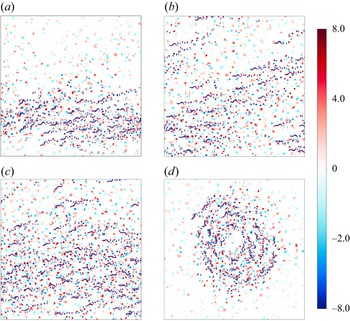
The swimming behaviour of fish, whether alone or in a group, is influenced by complex hydrodynamic forces. Previous studies on the collective behaviour of fish groups have often overlooked these hydrodynamic interactions (Kunz & Hemelrijk Reference Kunz and Hemelrijk2012; Calovi et al. Reference Calovi, Lopez, Schuhmacher, Chaté, Sire and Theraulaz2015), or estimated fluid forces using analytical methods, for example by superimposing vortex dipoles induced potential flows (Tchieu et al. Reference Tchieu, Kanso and Newton2012; Gazzola et al. Reference Gazzola, Tchieu, Alexeev, de Brauer and Koumoutsakos2016; Filella et al. Reference Filella, Nadal, Sire, Kanso and Eloy2018). In contrast, the hybrid model proposed in this study fully considers the intrinsic interplay between the locomotion of large-scale fish groups and hydrodynamic forces. Our hybrid model introduces an alternative approach by incorporating a more realistic hydrodynamic term into traditional SPP models. To illustrate the significance of this approach, we first present contour plots of the vorticity field for four representative modes in figure 9.

Figure 9.

Vorticity contours of four modes at the stable state: ( $a$ ) S0, tight schooling mode at $t/T=50$ ; ( $b$ ) S1, sparse schooling mode with $N=30$ at $t/T=58$ ; ( $c$ ) S2, sparse schooling mode with $N=50$ at $t/T=45$ ; ( $d$ ) M1, milling mode at $t/T=50$ . Here, $T$ denotes the initial undulation cycle, which is used to normalise the time in all results presented in this study. Supplemental movies S0, S1, S2 and M1 present dynamic evolutions of these modes.

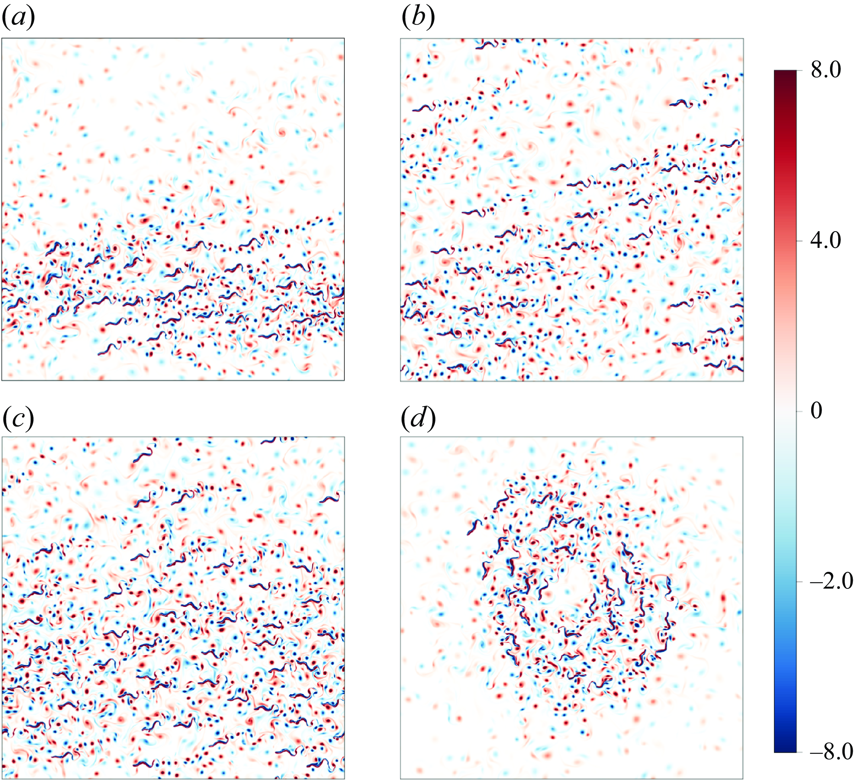
In the tight schooling mode (S0), the fish primarily aggregate and span only half of the computational domain, as shown in figure 9( $a$ ). The wake vortices generated by the swimmers create a relatively chaotic region that covers the lower half of the domain, while vortex disturbances are less evident in the upper areas. In the sparse schooling mode with 30 individuals (S1), shown in figure 9( $b$ ), the fish tend to cluster along the diagonal, with a few scattered individuals in the corners. This distribution results in flow disturbances that cover a larger area compared with mode S0. In the sparse schooling mode with 50 individuals (S2), depicted in figure 9( $c$ ), the fish are more uniformly distributed, leading to vortex structures that span the entire fluid domain. Finally, the milling mode (M1), characterised by a ring-like configuration, is markedly different from the schooling pattern, as shown in figure 9( $d$ ). The vortex disturbances in this mode align with the circular trajectory of the fish group, with the central region and areas far from the individuals being less affected by the induced vortices.

Importantly, in all modes, each individual swims through the vortex structures generated by its neighbours, indicating a strong coupling between the collective locomotion of the fish group and hydrodynamic effects. This highlights the essential role of incorporating hydrodynamic interactions into the modelling of fish groups to capture their fundamental and intrinsic features. The subsequent analyses on group formation structure, inter-group differences and individual differences are all based on this foundation.

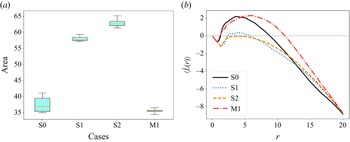
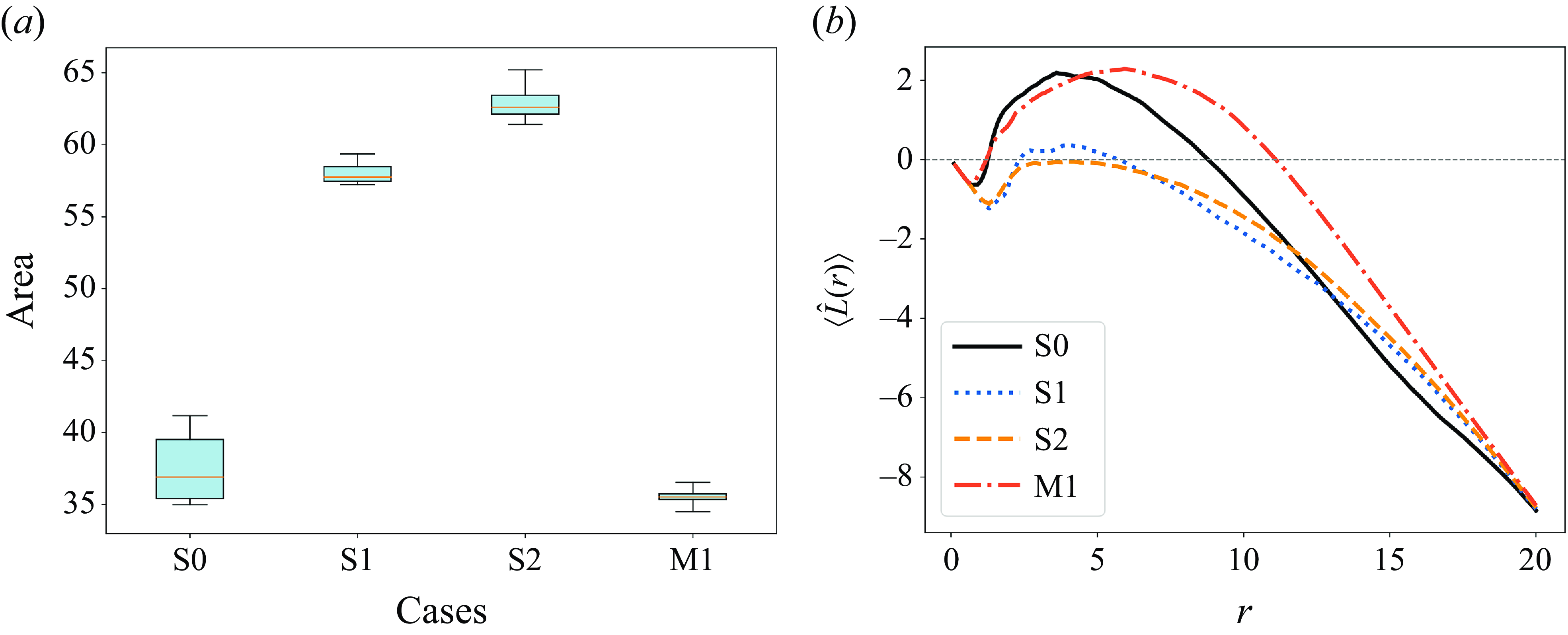
To differentiate between the tight and sparse modes, we employ two methods to quantitatively characterise group density across different modes. First, we measure the area occupied by the group using the convex hull structure, which indicates the distribution range of the fish group, as shown in figure 10( $a$ ). The data presented in the box plot are collected over a period from 40 $T$ to 60 $T$ , during which all modes reach a stable state. Due to differences in interaction intensity, the spatial distribution area of the two sparse schooling groups is approximately 56 $\%$ and 70 $\%$ larger than that of the right schooling group (see figure 10 $a$ ). The milling group, characterised by strong local attraction and a stable circular formation, occupies the smallest spatial area.

Next, we use Ripley’s $K$ function (Baggaley Reference Baggaley2015; Deng & Liu Reference Deng and Liu2021), a statistical pattern analysis method for measuring spatial clustering, to explore the variations in spatial structure among the four groups. Ripley’s $K$ function is defined as

(4.1)

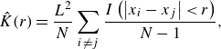\begin{equation} \hat {K}(r)=\frac {L^2}{N} \sum _{i \neq j} \frac {I\left (\left |x_i-x_j\right |\lt r\right )}{N-1}, \end{equation}

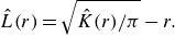
where $r$ is the spatial scale and $r \in [0, L]$ . Here, $I$ is the indicator function, which equals 1 if the Euclidean distance between points $i$ and $j$ is less than $r$ , and 0 otherwise. Furthermore, the Besag’s function can be obtained by normalising $\hat {K}(r)$ as follows:

(4.2)

\begin{equation} \hat {L}(r)=\sqrt {\hat {K}(r) / \pi }-r. \end{equation}

Besag’s function indicates a random distribution when it is zero, clustering of individuals over the spatial scale $r$ when positive and dispersion of individuals over a given scale when negative. Figure 10( $b$ ) presents the time-averaged Besag’s function for the four modes. It is evident that, due to the strong local attraction in the interaction rules, both the tight schooling group and the milling group exhibit a pronounced clustering pattern. In contrast, the two sparse schooling groups display looser formations, with individuals more uniformly distributed in space.

Figure 10.

( $a$ ) Box plots of the area occupied by the entire fish group, calculated based on the convex hull, over the time interval between $40T$ and $60T$ . These plots highlight the variations in spatial occupation over time. The central line in each box denotes the median, while the box itself represents the interquartile range, indicating the spread of the middle $50\, \%$ of the data. ( $b$ ) The time-averaged Besag function $\langle \hat {L}(r)\rangle$ for simulations of four groups, plotted as a function of spatial scale $r$ . A positive $\hat {L}(r)$ indicates clustering of individuals at a given scale, while a negative $\hat {L}(r)$ suggests segregation.

To further illustrate the differences between the four motion modes, we introduce two order parameters, $P$ and $M$ (Liu et al. Reference Liu, Liang, Deng and Zhang2023a )

(4.3)

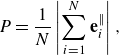\begin{equation} P=\frac {1}{N}\left |\sum _{i=1}^N \mathbf {e}_i^{\|}\right | ,\end{equation}

and

(4.4)

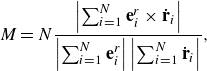\begin{equation} M=N \frac {\left |\sum _{i=1}^N \mathbf {e}_i^r \times \dot {\mathbf {r}}_i\right |}{\left |\sum _{i=1}^N \mathbf {e}_i^r\right |\left |\sum _{i=1}^N \dot {\mathbf {r}}_i\right |}, \end{equation}

where $N$ is the number of individuals, and $\mathbf {e}_i^r$ is the unit vector from the group’s centre of mass to the position of the $i$ th individual. The parameter $P$ represents the extent of group polarisation, and $M$ indicates the extent of milling. For a straight-line schooling formation, $P$ reaches a value of 1 and $M$ is zero, whereas in a perfect milling group, these values are reversed.

Figure 11.

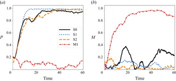
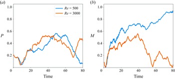
Time histories of order parameters $P$ and $M$ in four different modes: S0, S1, S2 and M1, with time non-dimensionalised by the initial undulatory period.

Figure 12.

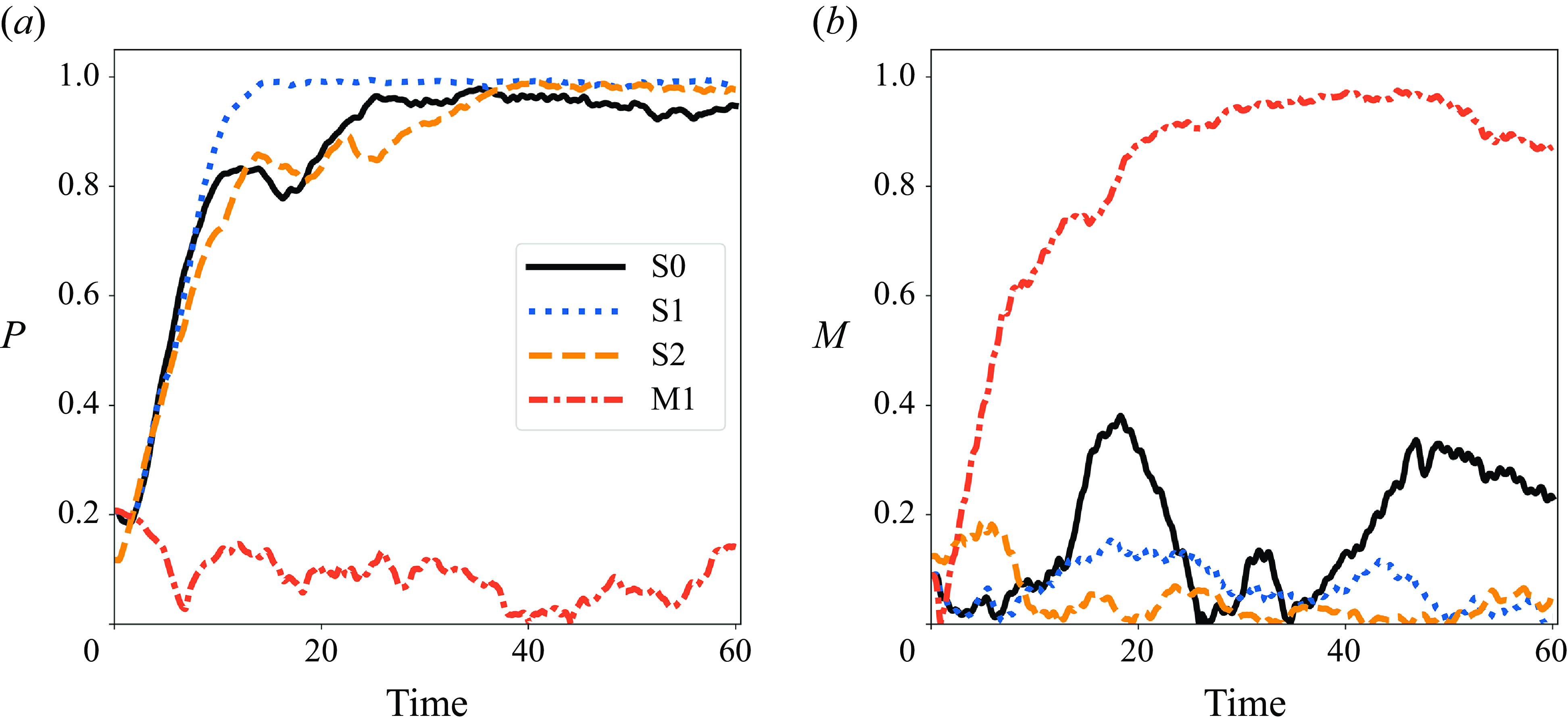
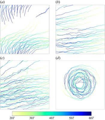
Illustration of individual trajectories in swimming groups for different modes: ( $a$ ) S0, ( $b$ ) S1, ( $c$ ) S2 and ( $d$ ) M1. The trajectory colours transition from light yellow to dark blue as time progresses, and the trajectories are recorded from 20 $T$ to 60 $T$ . Note that 20 $T$ marks the time when stable collective patterns emerge.

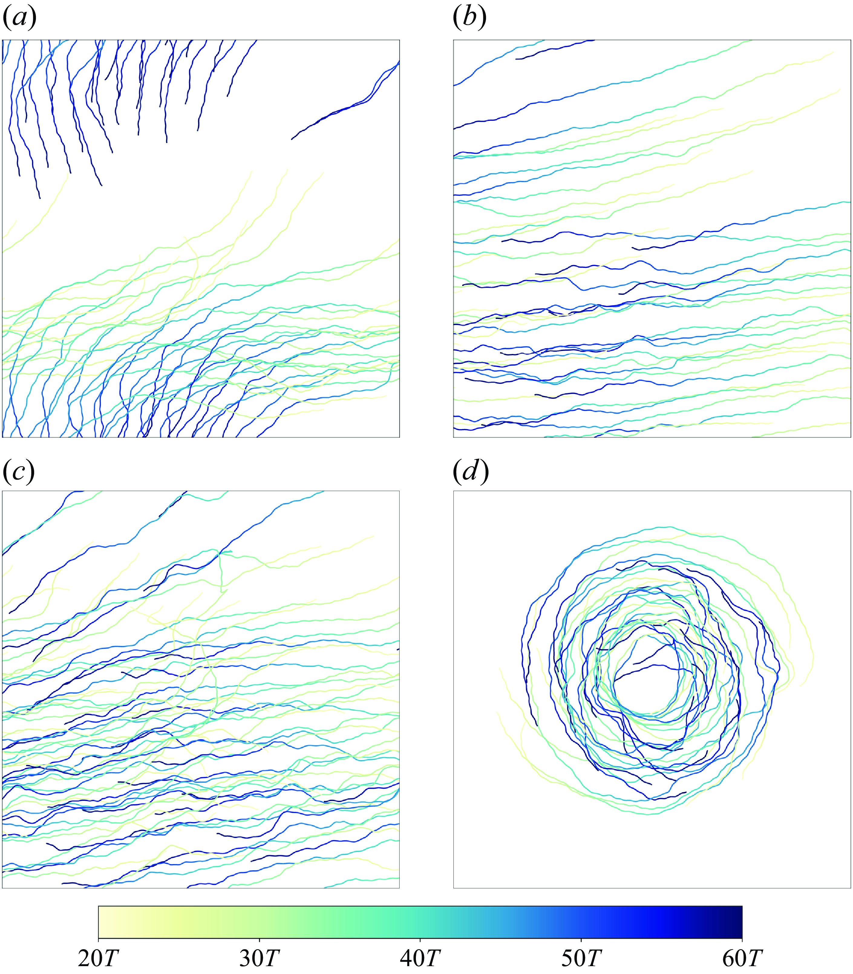
Figure 11 presents the time series of the order parameters $P$ and $M$ for the four different modes of fish group behaviour. These variations are reflected in the group trajectories shown in figure 12. When both the alignment intensity $a$ and local attraction intensity $c$ are relatively high, the fish group adopts a tight schooling mode, as seen in figure 12( $a$ ). This behaviour aligns well with the predictions of the SPP model, demonstrating highly coordinated collective motion. Over the period from 20 $T$ to 60 $T$ , the group maintains a high degree of alignment, as reflected in the order parameter $P$ , which approaches 1.0 by $t = 25T$ and remains nearly constant thereafter (see the black solid line for S0 in figure 11 $a$ ). A notable feature of this mode is the collective turning behaviour observed around $t=35T$ , where the group changes direction towards the lower left (see figure 12 $a$ ). This turning corresponds with a marked increase in the milling parameter $M$ starting at the same time (figure 11 $b$ ). Note that the initial rise in $M$ around $t = 10T$ is due to the fish adjusting their orientation, peaking at around $t=20T$ , after which the group tends to stabilise. Similar collective turning behaviour was reported by Filella et al. (Reference Filella, Nadal, Sire, Kanso and Eloy2018) when accounting for flow influence. Our findings are consistent with this observation, suggesting that such turning behaviour is indeed driven by hydrodynamic interactions.

In contrast, when the alignment term is moderate and the local attraction term is weak, the fish group forms a sparse schooling mode, as shown in figures 12( $b$ ) and ( $c$ ). Compared with the tight schooling mode, these sparse schooling modes display weaker cohesion among individuals and more dispersed formations, while still maintaining a high level of directional consistency. The primary distinction between modes S1 and S2 is the group size, with S1 having 30 individuals and S2 having 50 individuals. Despite following the same interaction rules, the increase in the number of individuals does not significantly impact the groups’ final formation. However, it is noteworthy that the large-scale group takes longer to reach a stable state, as shown in figure 11( $a$ ) (see the comparison between S1 and S2). In the S1 group, the order parameter $P$ quickly reaches a high value and fluctuates within a narrow range, while in the S2 group, $P$ fluctuates significantly between $t = 15T$ and $t = 40T$ . As figure 11( $b$ ) indicates, the parameter $M$ remains relatively low for both modes S1 and S2, suggesting that there is no turning tendency during the formation of these schooling modes.

For the milling mode, the group exhibits low global directional consistency. As shown in figure 11( $a$ ) for M1, the order parameter $P$ remains at a very low level throughout the entire process. Figure 12( $d$ ) shows the trajectories of the fish group in a stable milling mode, where the individuals rotate around a centre, resulting in a ring-like formation. The variation in parameter $M$ , as seen in figure 11( $b$ ), provides insights into the formation process of the milling mode. An initial ring structure forms at $t = 20T$ , and $M$ further increases as the collective motion undergoes dynamic adjustments. However, disturbances in the flow field can disrupt the orderly rotation, causing a decrease in $M$ . Consequently, the milling parameter $M$ stabilises at a fluctuating level, reflecting a balance between dynamic adjustments and flow field disturbances.

Figure 13.

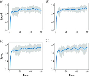
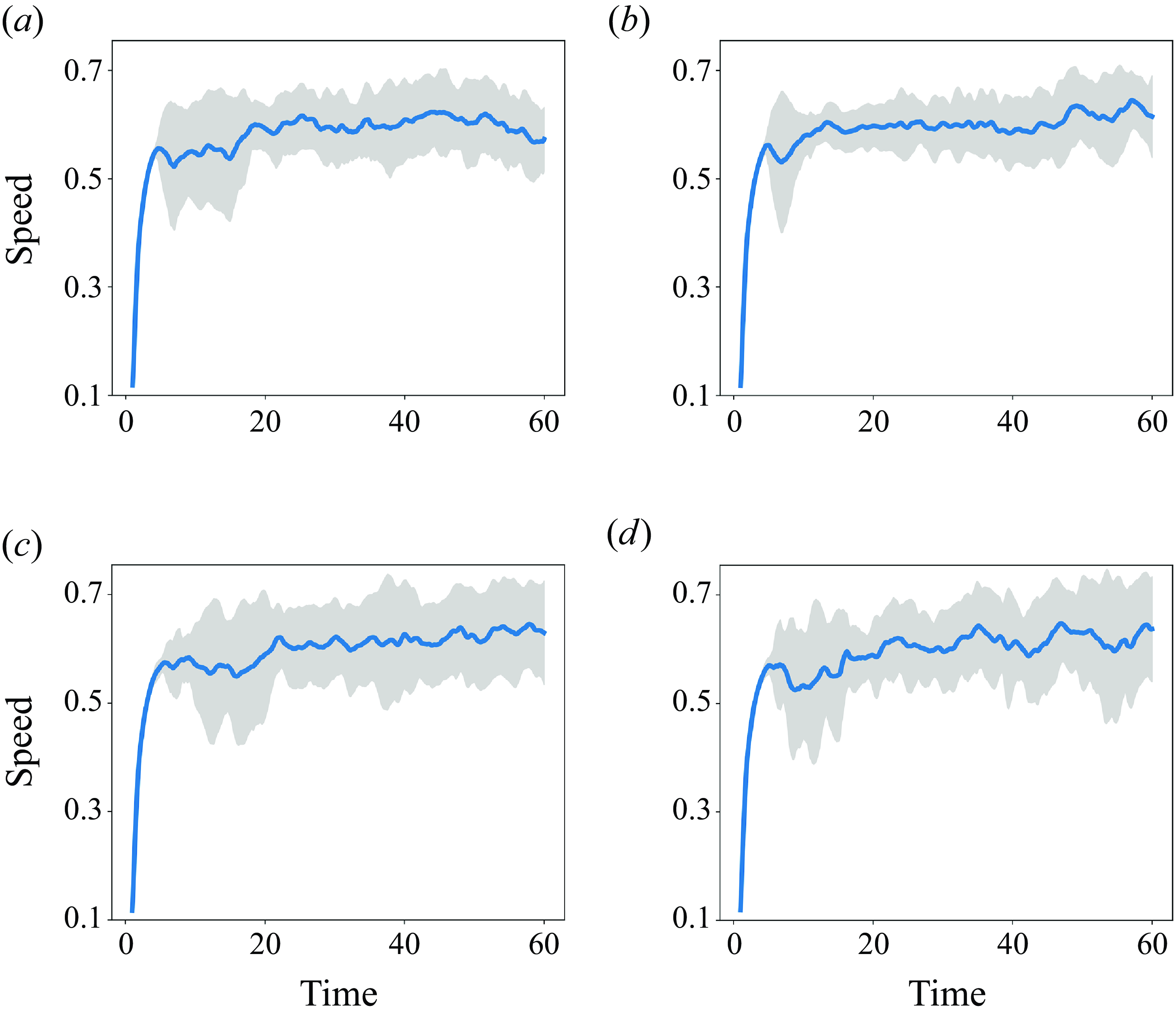
Individual speeds as a function of time for four different modes: ( $a$ ) S0, ( $b$ ) S1, ( $c$ ) S2 and ( $d$ ) M1, spanning from time 0 to 60 $T$ . The blue line represents the group’s average speed, smoothed using a moving average with a window of $T$ . The grey shaded area represents the standard deviation among individual speeds within the group, illustrating the variability in speed across different group members.

Figure 14.

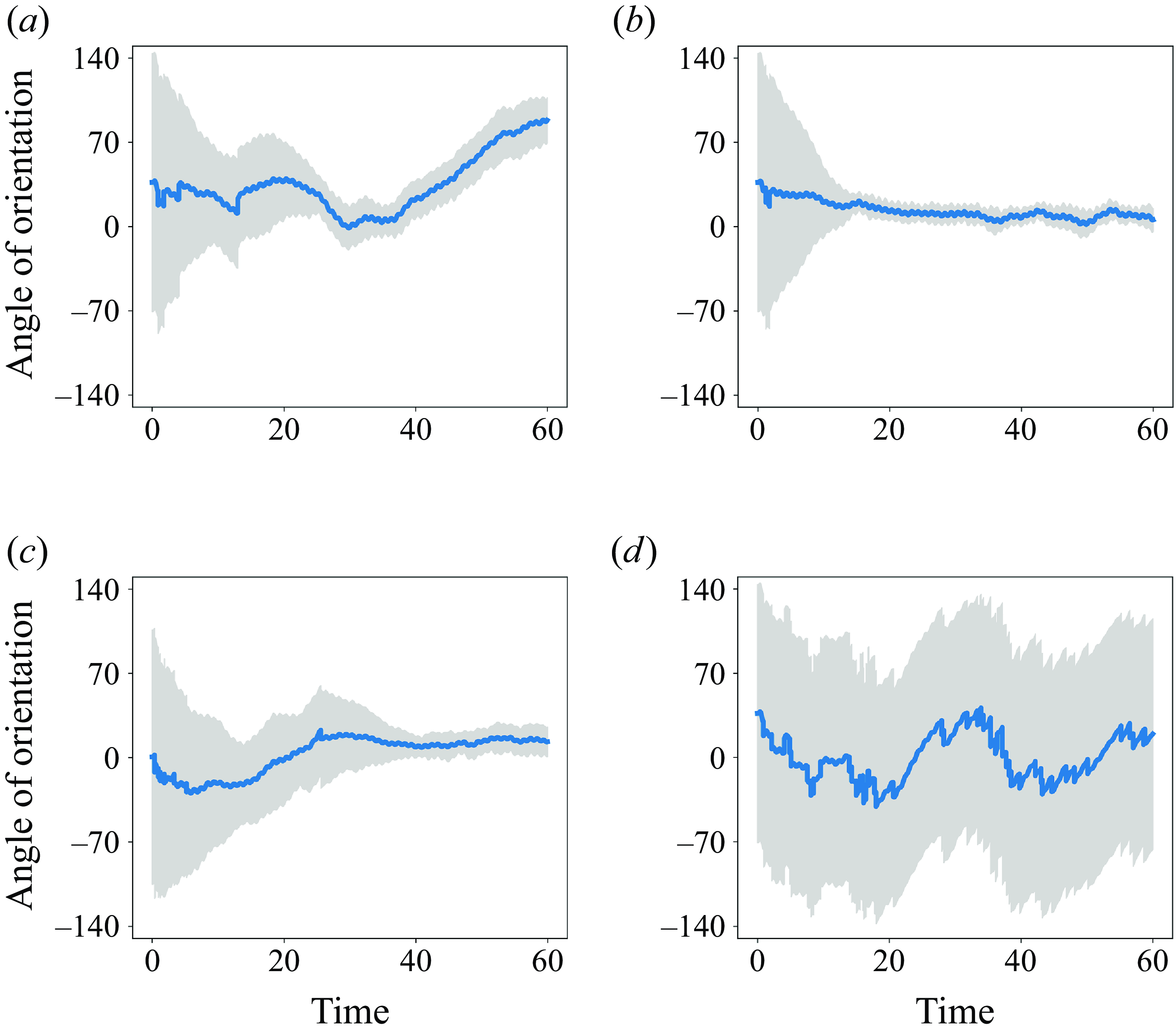
Time series of the oriented angle for four different modes: ( $a$ ) S0, ( $b$ ) S1, ( $c$ ) S2 and ( $d$ ) M1, spanning from time 0 to 60 $T$ . The blue line represents the group’s average angle of orientation, smoothed using a moving average with a window of $T$ . The grey shaded area represents the standard deviation of oriented angles among the individuals, indicating the variation in alignment within the group over time.

In previous models of fish schooling, individuals were typically represented as SPPs without inertia, swimming at a constant speed $v_0$ . Unlike models that completely ignore hydrodynamics, Filella et al. (Reference Filella, Nadal, Sire, Kanso and Eloy2018) acknowledged that fish are capable of sensing and exploiting flow features by incorporating an additional drift term into the interaction rules, allowing for variable swimming speeds. However, the calculation of this drift term was overly simplistic, approximating the influence of wake vortices induced by neighbours as a dipolar flow field. Another important limitation of these studies is that fish were simplified to points, neglecting the oscillatory swimming motion that causes speed fluctuations. In our computational approach, the test fish realistically undulate their bodies in the fluid, allowing the fish school to achieve more realistic speeds through self-propelled mechanisms driven by fluid forces. This enables direct comparisons of overall speed and individual speed discrepancies across different collective modes.

Figure 13 compares the individual swimming speeds across different modes. For fish groups in the schooling mode, individual speeds tend to converge towards around 0.6 when the order parameter $P$ approaches 1.0, regardless of group density. When comparing modes S1 and S2 (figures 13 $b$ and 13 $c$ ), we observe that speed variation among individuals tends to increase with group size. This suggests that larger fish groups create more complex flow fields, leading to greater variability in individual movements. In the milling mode, the average speed of the fish group aligns closely with that of the schooling groups, indicating that the flow fields generated by milling also contribute to an increase in individual speeds. The discrepancy of individual speeds highlights the significant impact of flow structures on movements in the milling collective motion.

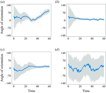
Figure 14 illustrates the variation in the moving direction of all individuals during the formation of a stable mode. The orientation angle plays a pivotal role in shaping the group’s formation, as the order parameters $P$ and $M$ are derived from this angle. For a fish group exhibiting the schooling mode, the relationship between figure 14( $a$ – $c$ ) and figure 11( $a$ ) is evident: a smaller grey shaded area in figure 14 corresponds to more consistent and aligned orientation angles among individuals, resulting in a higher $P$ value in figure 11. These findings indicate that the schooling pattern achieves a dynamic stability over time, whereas the milling group shows no evidence of alignment throughout its motion. The blue solid lines in figure 14 represent the group’s average direction of movement. Both the tightly coordinated schooling group and the milling group exhibit notable variations in their average moving direction during the motion, despite differences in their dynamic behaviours. In the schooling group, these variations signify collective turning behaviours, as shown in figure 14( $a$ ). In contrast, the directional data for the milling group reveal that the distribution of individuals is not uniformly or symmetrically maintained as they rotate around a central point. Importantly, the formation of the milling group remains dynamically variable throughout the collective motion.

The difference in movement direction between the two sparse groups, S1 (figure 14 $b$ ) and S2 (figure 14 $c$ ), suggests that, as the number of individuals increases, the group requires more time to achieve directionally consistent movement. This observation is supported by the changes in the parameter $P$ , as we have discussed above.

To briefly summarise, we employ the developed hybrid model to conduct a comprehensive analysis on the dynamical characteristics of fish groups in collective motion in this section. By fully considering hydrodynamic interactions, our study reveals some new observations about fish collective behaviour that differ significantly from previous studies relying on either analytical or empirical approaches to model fluid forces. Notably, the vorticity fields we provide underscore the critical importance of vortex-based interactions in modelling fish aggregation. The group trajectories presented here further demonstrate the robustness of our model in replicating typical collective formations observed in real fish groups. Additionally, our findings highlight the inherent differences and variability in both individual and group speeds, a factor often overlooked by traditional SPP models. It is important to note that the SPP method has been extensively developed over decades, resulting in various forms. In this study, we have selected one such variant to incorporate into our hybrid model. However, it remains an open question whether other SPP variants could serve a similar role.

4.2. Hydrodynamic benefits in collective locomotion

In this section, we explore the efficiency of fish swimming in groups by comparing different modes of collective motion using the CoT metric, defined as

(4.5)

\begin{equation} \mathrm {CoT}=\frac {\bar {P}}{U}, \end{equation}

where $\bar {P}$ represents the total motion power, and $U$ is the average speed (Liu et al. Reference Liu, Wang, Mao and Deng2023b ). The CoT measures the energy consumed per unit distance by a swimmer, with swimming efficiency inversely proportional to the CoT value. Therefore, a lower CoT indicates lower energy consumption and higher swimming efficiency.

Figure 15.

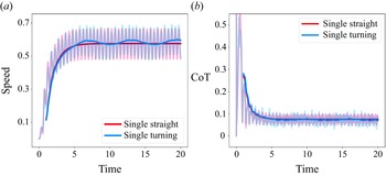
Numerical simulations of straight-line swimming (denoted as ‘single straight’) and continuous turning (denoted as ‘single turning’) of a single fish at the highest frequency $\omega =1.0$ and maximum undulatory amplitude ( $A=0.2$ ), with the parameter $B=0.2$ for the continuous turning (refer to (2.11) and (2.13)). ( $a$ ) Shows the speed of the fish, and ( $b$ ) presents the CoT efficiency. Dark lines indicate values averaged over the motion cycles.

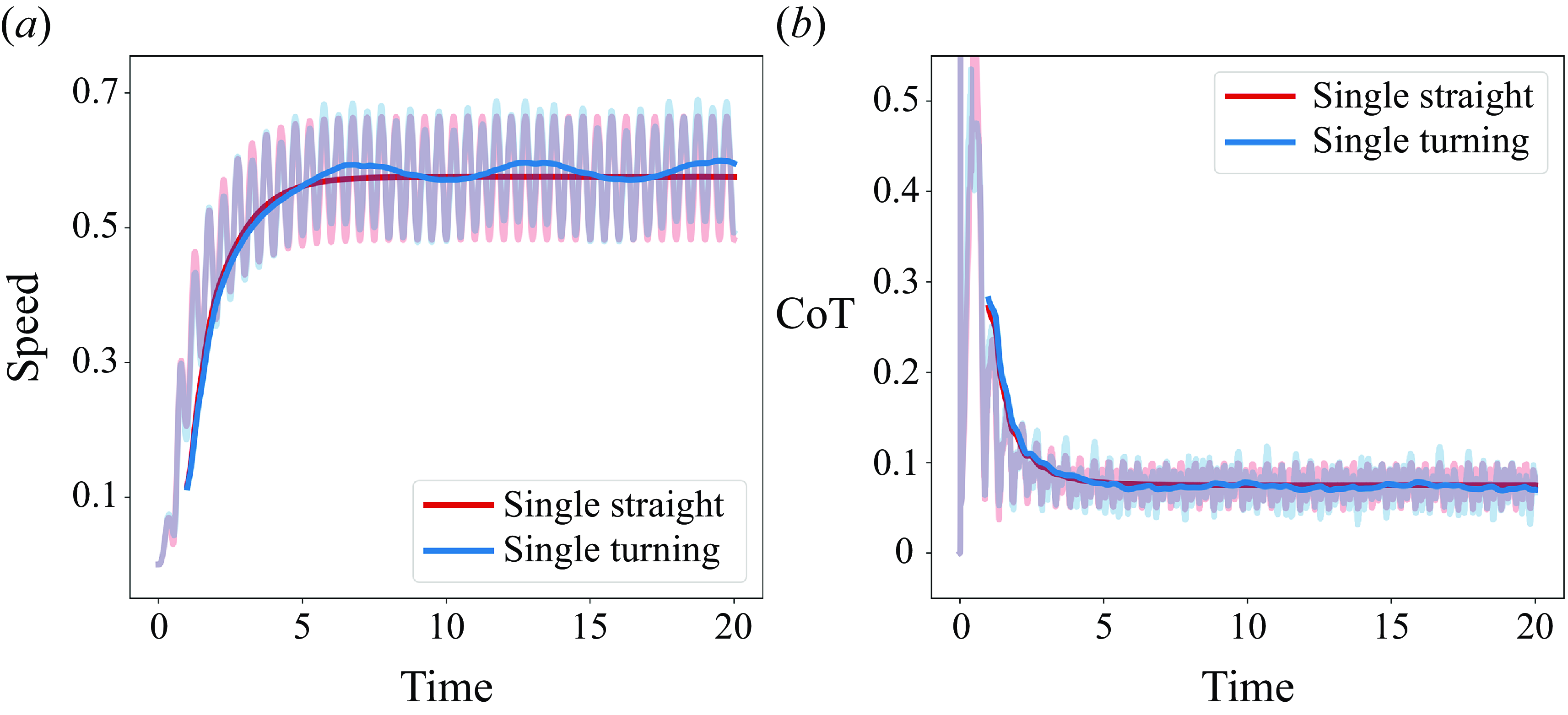
To understand the significance of collective behaviour, we first present the results of straight-line swimming and continuous turning of a solitary fish. For a direct comparison between solitary and group swimming, the amplitude and frequency of the single fish are set to match the initial settings used for the fish group. Figures 15( $a$ ) and 15( $b$ ) show the speed and CoT of a single fish swimming with the maximum undulatory amplitude (the initial setting for the fish group). After the initial acceleration phase, the cycle-averaged speed during straight-line swimming fish stabilises at $V=0.57$ with a CoT of 0.07588. For continuous turning at maximum turning capability, the speed and CoT stabilise at 0.58 and 0.07316, respectively.

Figure 16.

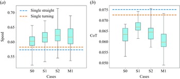
Box plots of ( $a$ ) swimming speed and ( $b$ ) CoT efficiency for four modes: S0, S1, S2 and M1, averaged from $40T$ to $60T$ . The data in each box represent time-averaged values for all individuals in the groups over this period. The dashed lines (blue for straight-line swimming and orange for continuous turning) represent the mean speed of a solitary swimmer.

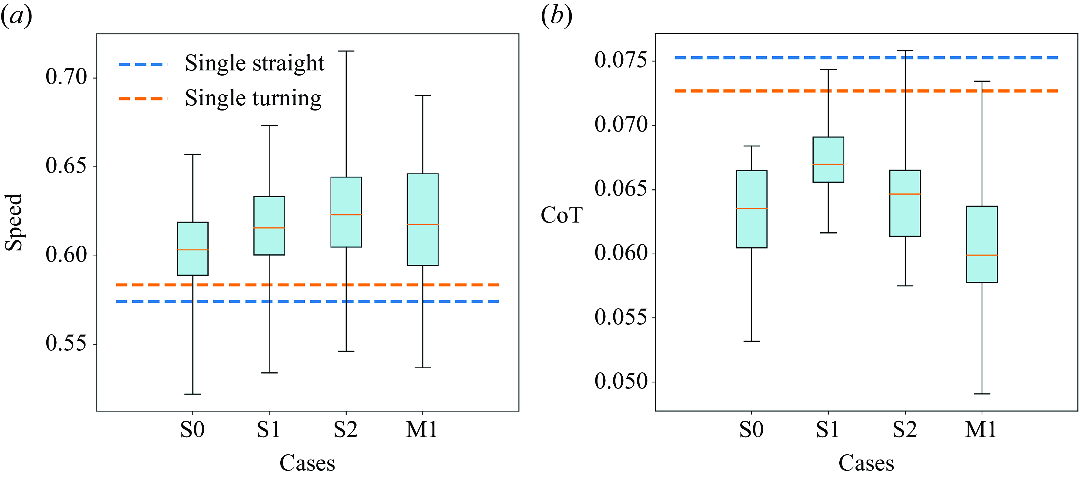
To further understand the hydrodynamic effects in different group modes, we present statistical data for the stable state (from 40 $T$ to 60 $T$ ) using box plots, as shown in figure 16. Figure 16( $a$ ) clearly shows that most individuals in both schooling and milling groups achieve speeds higher than those of a single fish swimming either in a straight line or while continuously turning. This indicates a significant collective advantage, where fish in a stable group mode benefit from increased speed. A similar pattern is observed in the efficiency results, as shown in figure 16( $b$ ). Compared with solitary swimming, all groups with collective motion demonstrate an evident energetic benefit.

On a collective level, this energetic benefit is influenced by group density. As seen in figure 16( $b$ ), the tight schooling and milling groups, characterised by more compact formations, exhibit lower energy consumption. Due to differences in group size, mode S2, with a larger number of individuals, results in a smaller average area occupied per individual, indicating higher density compared with mode S1, despite both being classified as sparse schooling under the same interaction rules. Consequently, the S2 group shows better energy efficiency than the S1 group.

Figure 17.

Scatter diagram of relative position in mode M1 for average values of ( $a$ ) speed and ( $b$ ) CoT efficiency from $40T$ to $60T$ . The diagram is presented in polar coordinates with the origin at the group centre. The red arrow points to a focused fish, labelled as A.

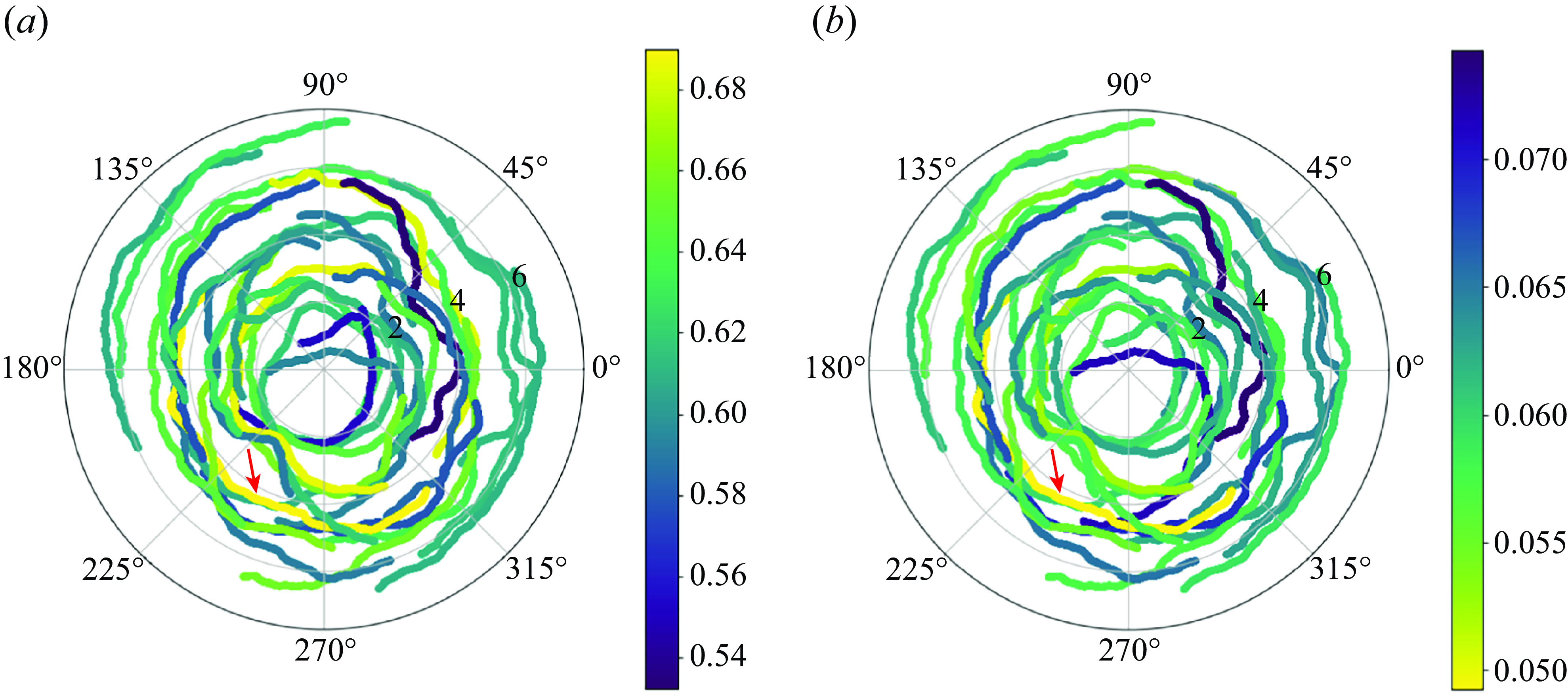
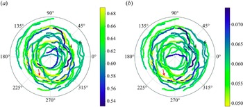
Taking the milling mode as an example, we explore the impact of hydrodynamic interactions on individual fish within the group. Figure 17 displays the swimming trajectories of each individual in the milling group during a stable period from 40 $T$ to 60 $T$ , plotted in polar coordinates with the origin at the group centre. The colours indicate different values of speed (figure 17 $a$ ) and CoT efficiency (figure 17 $b$ ). These results show significant differences in swimming speed and energy consumption based on individuals’ positions, which are evidently related to hydrodynamic effects. As mentioned earlier, the flow field fluctuations in the central region of the milling group are relatively small (figure 9 $d$ ). The fish passing through this region gain lower hydrodynamic benefits than the average level. 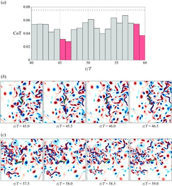In figure 17( $b$ ), we identify a particular individual, referred to as fish A, which achieves outstanding swimming efficiency during the considered period.

Figure 18.

Illustration of energy savings of fish A (referred to by an arrow in figure 17, and highlighted with green colour in this figure) by leveraging the macroscopic properties of the flow. ( $a$ ) The average CoT efficiency of fish A from 40 $T$ to 60 $T$ , with a dashed line marking the CoT value for a single continuous turning fish. The height of each square column represents the value averaged over each interval $T$ . Panels ( $b$ ) and ( $c$ ) show local vorticity contours around fish A for the two time periods highlighted in red in ( $a$ ).

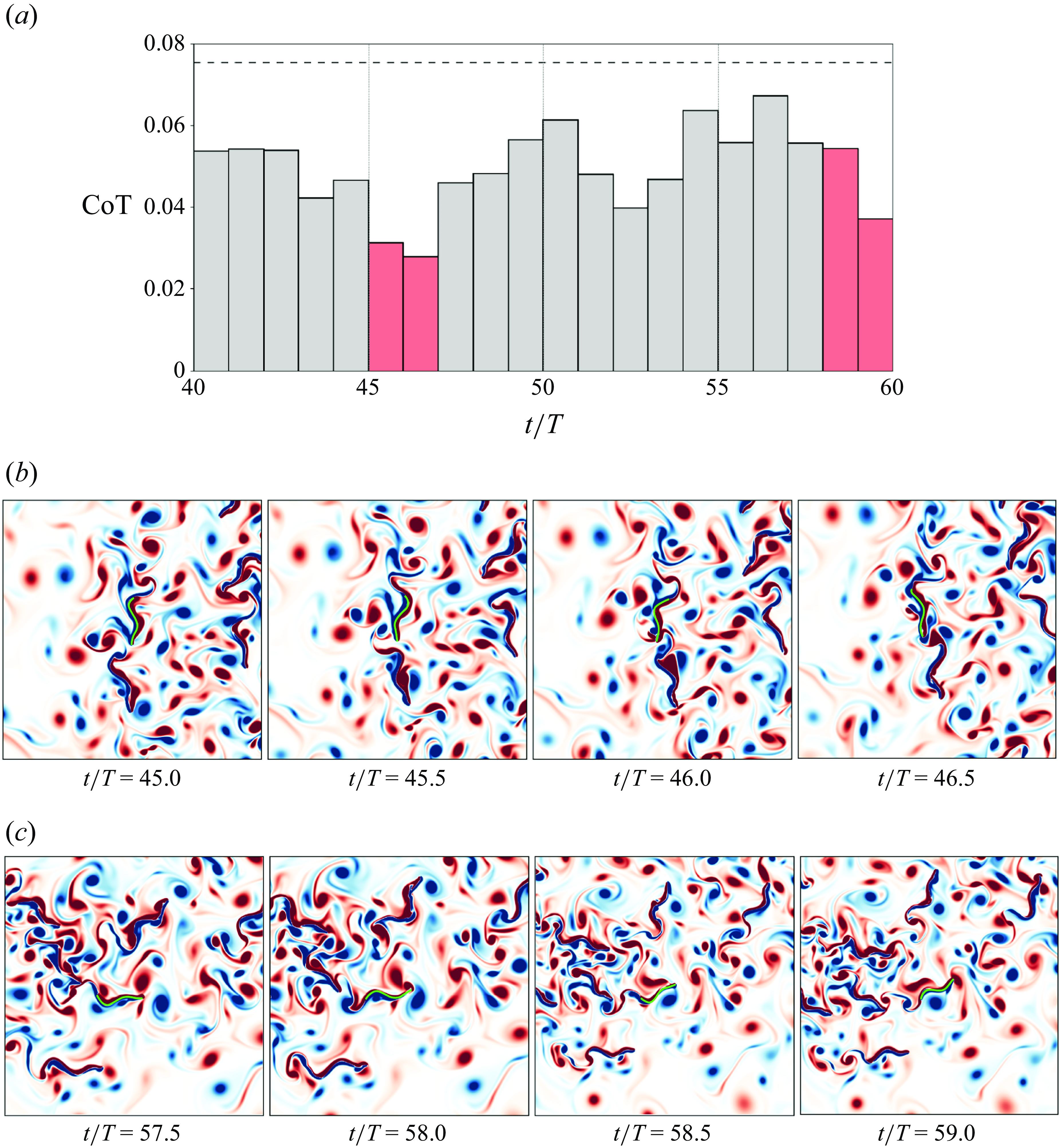
We further investigate how fish A becomes an efficient swimmer from a hydrodynamic perspective. Figure 18( $a$ ) shows the average CoT efficiency of fish A during each undulation cycle from 40 $T$ to 60 $T$ . It is clearly seen that fish A maintains a CoT lower than that of an isolated fish performing consistent turning throughout the entire period, suggesting continuous energetic benefits from collective motion. To uncover the underlying mechanism behind these hydrodynamic advantages, we select two notable phases with relatively low CoT (indicating higher swimming efficiency) for detailed flow field analysis. Figure 18( $b$ ) reveals that fish A acts as a follower, aligning with the leader in the same circular trajectory during the phase from $t/T = 45$ to $t/T = 46.5$ . In our previous study (Liu et al. Reference Liu, Wang, Mao and Deng2023b ), we demonstrated that, for two swimmers moving along a circular trajectory, the follower’s swimming efficiency is maximised when the radial spacing between the leader and follower is zero. Specifically, fish A, swimming in the same circle as the leader, can fully exploit the wake vortices generated by the leader, significantly saving energy during this period. During the phase from $t = 57.5T$ to $t = 59T$ , fish A is observed swimming through a pair of vortices moving in opposite directions. Interestingly, fish A’s swimming direction coincides with the velocity jet induced by these vortices, contributing to energy savings. Overall, the results in figures 18( $b$ ) and 18( $c$ ) indicate that the efficient swimming of fish A is due to the macroscopic properties of the flow, characterised by vortex motion and velocity distribution. These observations align well with previous studies attributing the benefits of collective motion to vortex-based interactions (Liao et al. Reference Liao, Beal, Lauder and Triantafyllou2003; Ashraf et al. Reference Ashraf, Bradshaw, Ha, Halloy, Godoy-Diana and Thiria2017) and velocity-based channelling effects (Daghooghi & Borazjani Reference Daghooghi and Borazjani2015). It is reasonable to expect that other individuals with high swimming efficiency experience similar hydrodynamic interactions.

It is important to emphasise that in our hybrid model, the SPP framework only considers simple interaction rules, as outlined in (2.3), and does not include any intelligent feedback mechanisms related to hydrodynamic forces or energy consumption. The hydrodynamic interactions in this model function purely as passive forces that influence the fish’s locomotion, as described in (2.17) and (2.18). Over time, it becomes increasingly plausible that these purely passive hydrodynamic interactions are sufficient to generate coherent collective locomotion and enhance the performance of the fish school (Ko et al. Reference Ko, Lauder and Nagpal2023). This elegant and simple hypothesis has its roots in the work of Lighthill and his collaborators (Weihs Reference Weihs1973; Lighthill Reference Lighthill1975; Weihs & Farhi Reference Weihs and Farhi2017). Recent experimental (Ashraf et al. Reference Ashraf, Godoy-Diana, Halloy, Collignon and Thiria2016, Reference Ashraf, Bradshaw, Ha, Halloy, Godoy-Diana and Thiria2017) and numerical studies (Dai et al. Reference Dai, He, Zhang and Zhang2018; Das, Peterson & Porfiri Reference Das, Peterson and Porfiri2023) have provided support for this conjecture. In our study, we are pleasantly surprised to discover that fish in collective motion groups indeed gain energetic benefits, as reflected by both their increased speed and lower CoT. It is worth noting that in our hybrid model simulations, the undulatory frequency and amplitude are always at or below those adopted in isolated fish swimming. In this regard, our findings lend further support to Lighthill’s conjecture.

4.3. Effects of Reynolds number on the collective motion

Previous studies using agent-based models have demonstrated the influence of hydrodynamic interactions on the collective behaviours of fish groups. However, those simplified hydrodynamic models are limited to either very low Reynolds numbers (Stokes flows) or infinite Reynolds numbers (inviscid flows) (Filella et al. Reference Filella, Nadal, Sire, Kanso and Eloy2018; Huang et al. Reference Huang, Ling and Kanso2024). As a result, critical information, such as the effects of Reynolds number and vortex scales in the swimming wakes, is lost. These factors are crucial for understanding both individual swimming performance in vortical flows and the collective behaviours of groups. To demonstrate the capability of our hybrid model in addressing these limitations, we investigate the effects of Reynolds number on the collective behaviours of fish groups.

To amplify the effects, we select a specific point at $a=0.7$ and $c=1.2$ , as marked in figure 7( $b$ ), located in the transition region between schooling and milling modes, where parameter sensitivity is higher. Two cases are simulated with identical interaction rules and initial conditions but at different Reynolds numbers: $Re\simeq 3000$ and $Re\simeq 500$ . Both cases involve a group of 30 individuals. The different Reynolds numbers are achieved by adjusting the viscosity $\mu$ , and the Reynolds number is calculated according to the average swimming speed of individuals as the groups reach quasi-steady states.

Figure 19.

Time histories of (a) $P$ and (b) $M$ for two fish groups with different Reynolds numbers. The blue lines represent $Re\simeq 500$ , and the orange lines indicate $Re\simeq 3000$ .

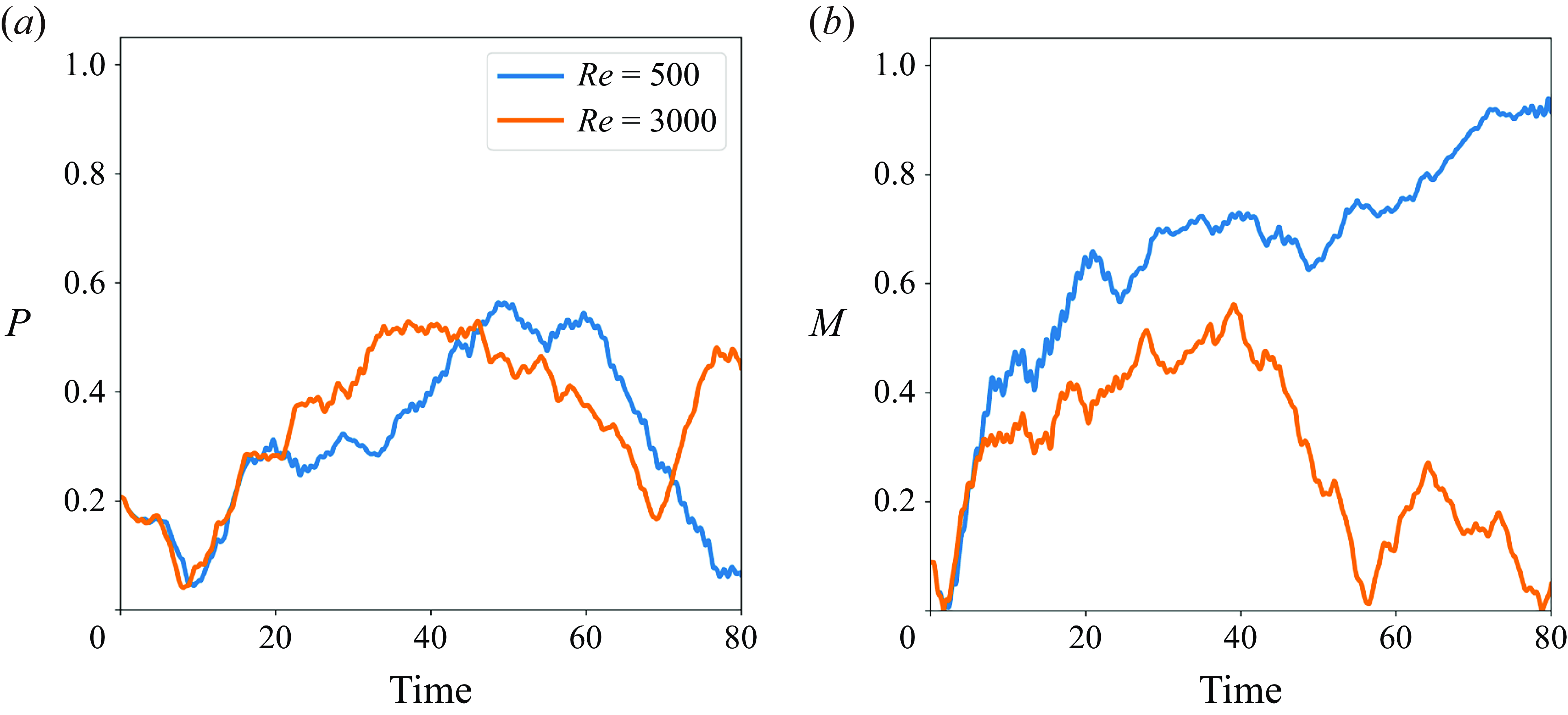
Figure 19 shows the time histories of the order parameters $P$ and $M$ for both cases. During the first $20T$ , the values of $P$ and $M$ are similar, reflecting consistent group motion due to identical initial conditions. However, as time progresses, significant differences emerge due to the influence of Reynolds number. For $Re\simeq 500$ , $M$ gradually increases while $P$ decreases, indicating a transition to a milling collective pattern. In contrast, for $Re\simeq 3000$ , both $P$ and $M$ remain relatively low, signifying a disordered group pattern deviating from milling or schooling configurations. These contrasting outcomes underscore the importance of incorporating environmental influences when modelling fish group dynamics and highlight the unique ability of the hybrid model to capture features not fully addressed by pure SPP models.

Figure 20.

Instantaneous vorticity contours of fish groups at $t = 65T$ for ( $a$ ) $Re\simeq 3000$ and ( $b$ ) $Re\simeq 500$ . The vortical field for the lower Reynolds number ( $Re\simeq 500$ ) shows a tighter milling pattern, whereas the wakes behind individuals appear more diffusive.

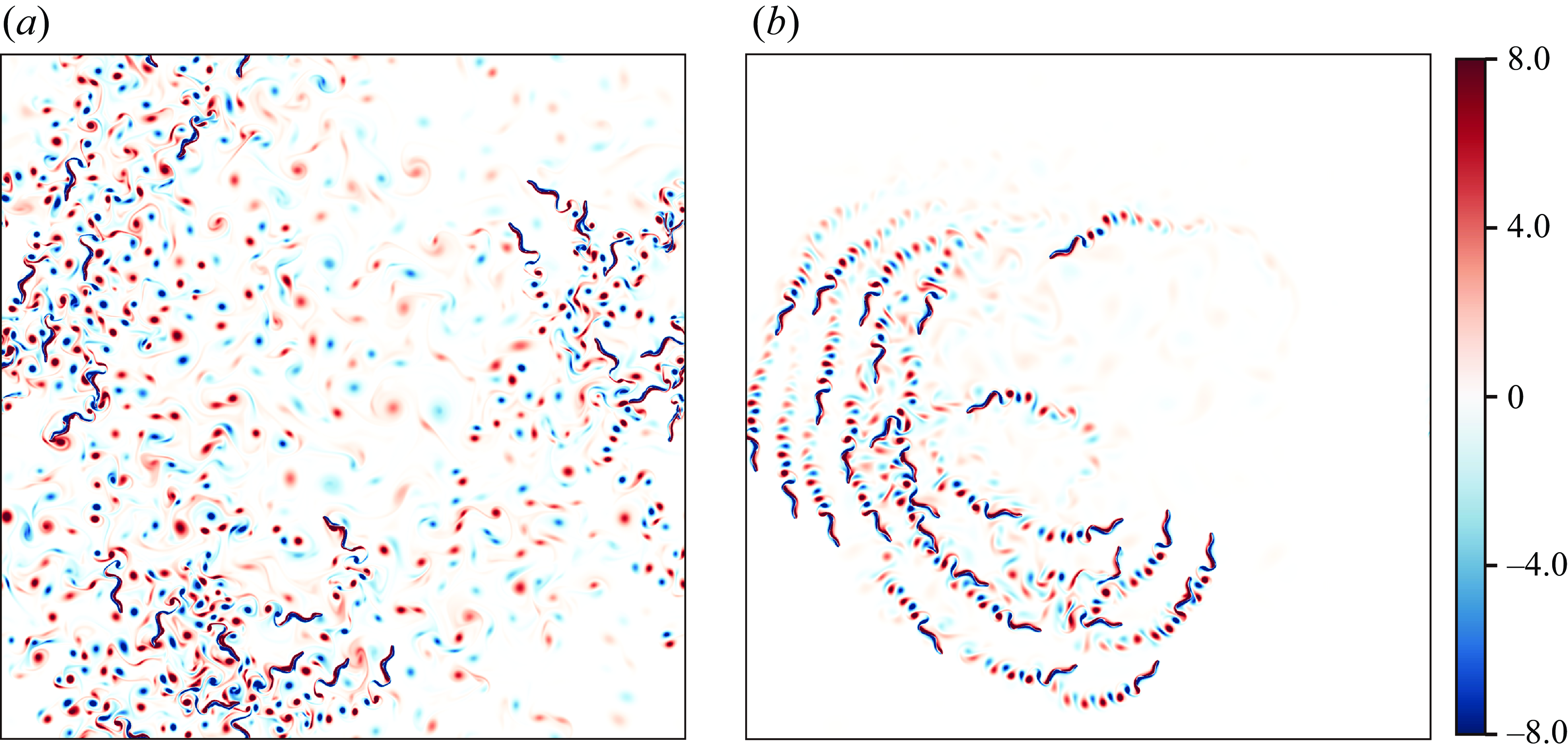
The instantaneous vorticity contours at $t = 65T$ (figure 20) further support these findings. At $Re\simeq 3000$ , the fish group exhibits chaotic flow patterns consistent with disordered group formations. In contrast, $Re\simeq 500$ produces a relatively organised flow pattern, aligning with a structured milling formation. The swimming speed of individuals depends on the balance between inertia and viscosity, while the resulting flow structures reciprocally influence locomotion. This strong coupling between locomotion and induced flow structures governs the evolution of group formation and determines the final group pattern. These underlying mechanisms emphasise the necessity of incorporating hydrodynamic impacts to uncover key behaviours in fish group dynamics.

5. Conclusions

In this study, we propose a hybrid numerical model that integrates the SPP method, which governs the local interactive rules between individuals to form specific collective configurations, with CFD simulations, where individual fish are modelled with active body undulation subjected to hydrodynamic forces imposed by their surrounding fluid flows. The coupling between the SPP model and CFD models is achieved through a CPG controller. Unlike previous agent-based models of fish groups, the primary significance of the developed model lies in its comprehensive consideration of hydrodynamic interactions, which play a crucial role in fish collective behaviours. Using this hybrid model, we conduct a series of simulations on both schooling and milling motions for large fish groups consisting of 30–50 individuals.

To demonstrate the capabilities of our hybrid model, we first explore the hydrodynamic effects on the collective behaviours of fish groups, effectively introducing an additional hydrodynamic term to the SPP model. Our results show that the fish groups can exhibit different collective modes depending on the coefficients of the SPP model, ranging from tight and sparse schooling to distinctive milling. We observe that the vorticity fields across all collective modes are characterised by significant vortex-vortex and vortex–fish interactions, giving rise to highly disturbed flow patterns. This finding underscores the necessity of incorporating vortex-based interactions in models of fish groups to uncover the underlying mechanisms governing collective behaviours.

Furthermore, due to the hydrodynamic interactions considered in our hybrid model, we find that both the swimming speed of individuals and the average speed of the entire group exhibit evident fluctuations, contrasting with the constant speeds typically assumed in traditional SPP models. We also examine the hydrodynamic benefits of collective locomotion. Comparisons between fish groups and solitary fish reveal that individuals in collective motion achieve higher swimming speeds and lower power expenditures. Notably, these hydrodynamic advantages become more pronounced as the group formation becomes more compact. A detailed flow field analysis indicates that the enhancement in swimming performance results from constructive vortex interactions and beneficial velocity distributions within the flow fields. Our observations align with the well-known hypotheses in the literature that suggest schooling fish gain hydrodynamic benefits from collective motion, thereby increasing their swimming efficiency.

The hybrid model proposed in this study provides a robust and reliable tool for investigating fish collective behaviours in large groups. However, it is important to acknowledge that this hybrid model represents only a preliminary framework for coupling agent-based models with CFD simulations and requires further development and validation. The insights gained from our observations are expected to advance the understanding of the intrinsic features of fish schooling and inform the design of bio-inspired underwater vehicles in group settings.

Our simulations are conducted in a two-dimensional (2-D) framework, which inherently imposes certain limitations in capturing the full complexity of real-world three-dimensional (3-D) fish collective behaviours. Numerous experiments and simulations have shown that 2-D wake vortices tend to persist longer than their 3-D counterparts, often exhibiting significant structural differences (Andersen et al. Reference Andersen, Bohr, Schnipper and Walther2017; Verma, Novati & Koumoutsakos Reference Verma, Novati and Koumoutsakos2018). Such distinctions can lead to notable variations in swimming efficiency for individual fish, particularly within specific formations like side-by-side or in-line arrangements (Pan et al. Reference Pan, Zhang, Kelly and Dong2024). Furthermore, the differences between 2-D and 3-D simulations extend to the spatial configuration of fish groups. Three-dimensional dynamics introduces vertical interactions and positioning effects that are absent in 2-D models. For instance, our previous work observed a 3-D bait ball configuration in collective fish motion using a solely SPP model (Liu et al. Reference Liu, Liang, Deng and Zhang2023a ). In contrast, the current 2-D hybrid model produces a circular planar configuration. While the present 2-D model effectively captures the collective motion of fish within a plane, the influence of 3-D dynamics becomes significant when the vertical distance between individuals is comparable to the fish length (Li et al. Reference Li, Zheng, Mao and Xie2021b ). Therefore, to enhance the fidelity and applicability of these findings, future studies should consider the development and application of a 3-D hybrid model. However, it is worth noting that many experimental investigations into fish collective behaviour have been conducted in shallow water tanks to facilitate observation (Lafoux et al. Reference Lafoux, Moscatelli, Godoy-Diana and Thiria2023). As such, the present 2-D model may still provide valuable insights for interpreting these quasi-2-D experimental scenarios.

Future research could build upon this work by exploring aspects such as kinematic variability among individuals, the influence of fish shape, 3-D effects and the impact of turbulence. However, a balance must always be maintained between the computational cost associated with fluid simulation and the model’s realism. Additionally, an intriguing direction for the development of this hybrid model would involve incorporating multiple sensors, as suggested by Ko et al. (Reference Ko, Lauder and Nagpal2023), and introducing reinforcement learning strategies. This would allow for the study of how agents actively respond to hydrodynamic cues and how variations in feedback mechanisms influence group cohesiveness.

Supplementary movies

Supplementary movies are available at https://doi.org/10.1017/jfm.2025.216.

Funding

This research has been supported by the National Natural Science Foundation of China (Grants No. 92252102 and No. 123B1001).

Declaration of interests

The authors report no conflict of interest.

References

Alben, S. 2021 Collective locomotion of two-dimensional lattices of flapping plates. Part 2. Lattice flows and propulsive efficiency. J. Fluid Mech. 915, A21.CrossRef Google Scholar

Andersen, A., Bohr, T., Schnipper, T. & Walther, J.H. 2017 Wake structure and thrust generation of a flapping foil in two-dimensional flow. J. Fluid Mech. 812, R4.CrossRef Google Scholar

Arranz, G., Flores, O. & García-Villalba, M. 2022 Flow interaction of three-dimensional self-propelled flexible plates in tandem. J. Fluid Mech. 931, A5.CrossRef Google Scholar

Ashraf, I., Bradshaw, H., Ha, T.-T., Halloy, J., Godoy-Diana, R. & Thiria, B. 2017 Simple phalanx pattern leads to energy saving in cohesive fish schooling. Proc. Natl Acad. Sci. USA 114 (36), 9599–9604.CrossRef Google Scholar PubMed

Ashraf, I., Godoy-Diana, R., Halloy, J., Collignon, B. & Thiria, B. 2016 Synchronization and collective swimming patterns in fish (Hemigrammus bleheri). J. R. Soc. Interface 13 (123), 20160734.CrossRef Google Scholar PubMed

Baggaley, A.W. 2015 Model flocks in a steady vortical flow. Phys. Rev. E 91 (5), 053019.CrossRef Google Scholar

Ballerini, M. et al. 2008 Interaction ruling animal collective behavior depends on topological rather than metric distance: evidence from a field study. Proc. Natl Acad. Sci. USA 105 (4), 1232–1237.CrossRef Google Scholar PubMed

Bao, Y., Zhou, D., Tao, J.J., Peng, Z., Zhu, H.B., Sun, Z.L. & Tong, H.L. 2017 Dynamic interference of two anti-phase flapping foils in side-by-side arrangement in an incompressible flow. Phys. Fluids 29 (3), 033601.CrossRef Google Scholar

Bastien, R. & Romanczuk, P. 2020 A model of collective behavior based purely on vision. Sci. Adv. 6 (6), eaay0792.CrossRef Google Scholar

Boschitsch, B.M., Dewey, P.A. & Smits, A.J. 2014 Propulsive performance of unsteady tandem hydrofoils in an in-line configuration. Phys. Fluids 26 (5), 051901.CrossRef Google Scholar

Brock, V.E. & Riffenburgh, R.H. 1960 Fish schooling: a possible factor in reducing predation. ICES J. Mar. Sci. 25 (3), 307–317.CrossRef Google Scholar

Calovi, D.S., Lopez, U., Ngo, S., Sire, C., Chaté, H. & Theraulaz, G. 2014 Swarming, schooling, milling: phase diagram of a data-driven fish school model. New J. Phys. 16 (1), 015026.CrossRef Google Scholar

Calovi, D.S., Lopez, U., Schuhmacher, P., Chaté, H., Sire, C. & Theraulaz, G. 2015 Collective response to perturbations in a data-driven fish school model. J. R. Soc. Interface 12 (104), 20141362.CrossRef Google Scholar

Camperi, M., Cavagna, A., Giardina, I., Parisi, G. & Silvestri, E. 2012 Spatially balanced topological interaction grants optimal cohesion in flocking models. Interface Focus 2 (6), 715–725.CrossRef Google Scholar PubMed

Carling, J., Williams, T.L. & Bowtell, G. 1998 Self-propelled anguilliform swimming: simultaneous solution of the two-dimensional Navier–Stokes equations and Newton’s laws of motion. J. Exp. Biol. 201 (23), 3143–3166.CrossRef Google Scholar PubMed

Cavagna, A., Cimarelli, A., Giardina, I., Parisi, G., Santagati, R., Stefanini, F. & Tavarone, R. 2010 From empirical data to inter-individual interactions: unveiling the rules of collective animal behavior. Math. Models Meth. Appl. Sci. 20 (supp01), 1491–1510.CrossRef Google Scholar

Chaté, H., Ginelli, F., Grégoire, G., Raynaud, F. 2008 Collective motion of self-propelled particles interacting without cohesion. Phys. Rev. E 77 (4), 046113.CrossRef Google Scholar PubMed

Chen, S.-Y., Fei, Y.-H.J., Chen, Y.-C., Chi, K.-J. & Yang, J.-T. 2016 The swimming patterns and energy-saving mechanism revealed from three fish in a school. Ocean Engng 122, 22–31.CrossRef Google Scholar

Cushing, D.H. & Jones, F.R.H. 1968 Why do fish school? Nature 218 (5145), 918–920.CrossRef Google Scholar PubMed

Daghooghi, M. & Borazjani, I. 2015 The hydrodynamic advantages of synchronized swimming in a rectangular pattern. Bioinspir. Biomim. 10 (5), 056018.CrossRef Google Scholar

Dai, L., He, G., Zhang, X. & Zhang, X. 2018 Stable formations of self-propelled fish-like swimmers induced by hydrodynamic interactions. J. R. Soc. Interface 15 (147), 20180490.CrossRef Google Scholar PubMed

Das, R., Peterson, S.D. & Porfiri, M. 2023 Stability of schooling patterns of a fish pair swimming against a flow. Flow 3, E31.CrossRef Google Scholar

De Lellis, P. & Porfiri, M. 2022 Inferring the size of a collective of self-propelled Vicsek particles from the random motion of a single unit. Commun. Phys. 5 (1), 86.CrossRef Google Scholar

Deng, J. & Liu, D. 2021 Spontaneous response of a self-organized fish school to a predator. Bioinspir. Biomim. 16 (4), 046013.CrossRef Google Scholar PubMed

Deng, J., Mao, X. & Xie, F. 2019 Dynamics of two-dimensional flow around a circular cylinder with flexible filaments attached. Phys. Rev. E 100 (5), 053107.CrossRef Google Scholar PubMed

Deng, J. & Shao, X.-M. 2006 Hydrodynamics in a diamond-shaped fish school. J. Hydrodyn. 18 (S1), 428–432.CrossRef Google Scholar

Deng, J., Shao, X.-M. & Yu, Z.-S. 2007 Hydrodynamic studies on two traveling wavy foils in tandem arrangement. Phys. Fluids 19 (11), 113104.CrossRef Google Scholar

Dong, G.-J. & Lu, X.-Y. 2007 Characteristics of flow over traveling wavy foils in a side-by-side arrangement. Phys. Fluids 19 (5), 057107.CrossRef Google Scholar

Escobedo, R., Lecheval, V., Papaspyros, V., Bonnet, F., Mondada, F., Sire, C. & Theraulaz, G. 2020 A data-driven method for reconstructing and modelling social interactions in moving animal groups. Phil. Trans. R. Soc. Lond. B: Biol. Sci. 375 (1807), 1807,–20190380.CrossRef Google Scholar PubMed

Filella, A., Nadal, F., Sire, C., Kanso, E. & Eloy, C. 2018 Model of collective fish behavior with hydrodynamic interactions. Phys. Rev. Lett. 120 (19), 198101.CrossRef Google Scholar PubMed

Gautrais, J., Ginelli, F., Fournier, R., Blanco, S., Soria, M., Chaté, H. & Theraulaz, G. 2012 Deciphering interactions in moving animal groups. PLoS Computational Biology 8 (9), e1002678.CrossRef Google Scholar PubMed

Gautrais, J., Jost, C., Soria, M., Campo, A., Motsch, S., Fournier, R., Blanco, S. & Theraulaz, G. 2009 Analyzing fish movement as a persistent turning walker. J. Math. Biol. 58 (3), 429–445.CrossRef Google Scholar PubMed

Gazzola, M., Tchieu, A A., Alexeev, D., de Brauer, A. & Koumoutsakos, P. 2016 Learning to school in the presence of hydrodynamic interactions. J. Fluid Mech. 789, 726–749.CrossRef Google Scholar

Ginelli, F. 2016 The physics of the Vicsek model. Eur. Phys. J. Special Topics 225 (11-12), 2099–2117.CrossRef Google Scholar

Ginelli, F. & Chaté, H. 2010 Relevance of metric-free interactions in flocking phenomena. Phys. Rev. Lett. 105 (16), 168103.CrossRef Google Scholar PubMed

Goldstein, D., Handler, R. & Sirovich, L. 1993 Modeling a no-slip flow boundary with an external force field. J. Comput. Phys. 105 (2), 354–366.CrossRef Google Scholar

Grégoire, G., Chaté, H. & Tu, Y. 2003 Moving and staying together without a leader. Physica D: Nonlinear Phenom. 181 (3-4), 157–170.CrossRef Google Scholar

Hemelrijk, C.K., Reid, D.A.P., Hildenbrandt, H. & Padding, J.T. 2015 The increased efficiency of fish swimming in a school. Fish Fish 16 (3), 511–521.CrossRef Google Scholar

Heydari, S. & Kanso, E. 2021 School cohesion, speed and efficiency are modulated by the swimmers flapping motion. J. Fluid Mech. 922, A27.CrossRef Google Scholar

Huang, C., Ling, F. & Kanso, E. 2024 Collective phase transitions in confined fish schools. Proc. Natl Acad. Sci. USA 121(44), e2406293121.CrossRef Google Scholar PubMed

Ioannou, C.C., Guttal, V. & Couzin, I.D. 2012 Predatory fish select for coordinated collective motion in virtual prey. Science 337 (6099), 1212–1215.CrossRef Google Scholar PubMed

Kanso, E. & Newton, P.K. 2010 Locomotory advantages to flapping out of phase. Expl. Mech. 50 (9), 1367–1372.CrossRef Google Scholar

Kanso, E. & Tsang, A.C.H. 2014 Dipole models of self-propelled bodies. Fluid Dyn. Res. 46 (6), 061407.CrossRef Google Scholar

Khalid, M.S.U., Akhtar, I. & Dong, H. 2016 Hydrodynamics of a tandem fish school with asynchronous undulation of individuals. J. Fluid Struct. 66, 19–35.CrossRef Google Scholar

Ko, H., Lauder, G. & Nagpal, R. 2023 The role of hydrodynamics in collective motions of fish schools and bioinspired underwater robots. J. R. Soc. Interface 20 (207), 20230357.CrossRef Google Scholar PubMed

Krebs, J.R., MacRoberts, M.H. & Cullen, J.M. 1972 Flocking and feeding in the great tit parus major–an experimental study. Ibis 114 (4), 507–530.CrossRef Google Scholar

Kunz, H. & Hemelrijk, C.K. 2012 Simulations of the social organization of large schools of fish whose perception is obstructed. Appl. Animal Behav. Sci. 138 (3-4), 142–151.CrossRef Google Scholar

Lafoux, B., Moscatelli, J., Godoy-Diana, R. & Thiria, B. 2023 Illuminance-tuned collective motion in fish. Commun. Biol. 6 (1), 585.CrossRef Google Scholar PubMed

Landeau, L. & Terborgh, J. 1986 Oddity and the confusion effectin predation. Animal Behav. 34 (5), 1372–1380.CrossRef Google Scholar

Lazarus, J. 1979 The early warning function of flocking in birds: an experimental study with captive quelea. Animal Behav. 27, 855–865.CrossRef Google Scholar

Li, G., Kolomenskiy, D., Liu, H., Thiria, B., Godoy-Diana, R. & Gurka, R. 2019 On the energetics and stability of a minimal fish school. PLoS One 14 (8), e0215265.CrossRef Google Scholar PubMed

Li, L., Liu, D., Deng, J., Lutz, M.J. & Xie, G. 2021 a Fish can save energy via proprioceptive sensing. Bioinspir. Biomim. 16 (5), 056013.CrossRef Google Scholar PubMed

Li, L., Zheng, X., Mao, R. & Xie, G. 2021 b Energy saving of schooling robotic fish in three-dimensional formations. IEEE Robot. Autom. Lett. 6 (2), 1694–1699.CrossRef Google Scholar

Liao, J.C., Beal, D.N., Lauder, G.V. & Triantafyllou, M.S. 2003 Fish exploiting vortices decrease muscle activity. Science 302 (5650), 1566–1569.CrossRef Google Scholar PubMed

Lighthill, S.J. 1975 Mathematical biofluiddynamics. SIAM.CrossRef Google Scholar

Ligman, M., Lund, J. & Fürth, M. 2024 A comprehensive review of hydrodynamic studies on fish schooling. Bioinspir. Biomim. 19 (1), 011002.CrossRef Google Scholar

Lin, X., Wu, J., Zhang, T. & Yang, L. 2020 Self-organization of multiple self-propelling flapping foils: energy saving and increased speed. J. Fluid Mech. 884, R1.CrossRef Google Scholar

Lin, X., Wu, J., Zhang, T. & Yang, L. 2021 Flow-mediated organization of two freely flapping swimmers. J. Fluid Mech. 912, A37.CrossRef Google Scholar

Ling, H., Mclvor, G.E., Westley, J., van der Vaart, K., Vaughan, R.T., Thornton, A.& Ouellette, N.T. 2019 Behavioural plasticity and the transition to order in jackdaw flocks. Nat. Commun. 10 (1), 5174.CrossRef Google Scholar PubMed

Liu, D., Liang, Y., Deng, J. & Zhang, W. 2023 a Modeling three-dimensional bait ball collective motion. Phys. Rev. E 107 (1), 014606.CrossRef Google Scholar PubMed

Liu, D., Wang, J., Mao, X. & Deng, J. 2023 b Energetic benefits in coordinated circular swimming motion of two swimmers. Phys. Rev. E 108 (5), 054603.CrossRef Google Scholar PubMed

Liu, X., Liu, K. & Huang, H. 2022 Collective behavior and hydrodynamic advantage of side-by-side self-propelled flapping foils. Phys. Rev. E 105 (6), 065105.CrossRef Google Scholar PubMed

Lopez, U., Gautrais, J., Couzin, I.D. & Theraulaz, G. 2012 From behavioural analyses to models of collective motion in fish schools. Interface Focus 2 (6), 693–707.CrossRef Google Scholar PubMed

Mudaliar, R.K., Zvezdin, A.V., Bratt, G.S. & Schaerf, T.M. 2022 Systematic analysis of emergent collective motion produced by a 3D hybrid zonal model. Bull. Math. Biol. 84 (1), 1–25.Google Scholar PubMed

Pan, Y., Zhang, W., Kelly, J. & Dong, H. 2024 Unraveling hydrodynamic interactions in fish schools: a three-dimensional computational study of in-line and side-by-side configurations. Phys. Fluids 36 (8), 081909.CrossRef Google Scholar

Peng, Z.-R., Huang, H. & Lu, X.-Y. 2018 Hydrodynamic schooling of multiple self-propelled flapping plates. J. Fluid Mech. 853, 587–600.CrossRef Google Scholar

Pitcher, T.J., Magurran, A.E. & Winfield, I.J. 1982 Fish in larger shoals find food faster. Behav. Ecol. Sociobiol. 10 (2), 149–151.CrossRef Google Scholar

Romanczuk, P., Couzin, I.D. & Schimansky-Geier, L. 2009 Collective motion due to individual escape and pursuit response. Phys. Rev. Lett. 102 (1), 010602.CrossRef Google Scholar PubMed

Roy, S. & Lemus, J. 2021 How does the fusion of sensory information from audition and vision impact collective behavior? Frontiers Appl. Maths Stat. 7, 758711.CrossRef Google Scholar

Sánchez-Rodríguez, J.A., Raufaste, C. & Argentina, M. 2023 Scaling the tail beat frequency and swimming speed in underwater undulatory swimming. Nat. Commun. 14 (1), 5569.CrossRef Google Scholar PubMed

Shirgaonkar, A.A., MacIver, M.A. & Patankar, N.A. 2009 A new mathematical formulation and fast algorithm for fully resolved simulation of self-propulsion. J. Comput. Phys. 228 (7), 2366–2390.CrossRef Google Scholar

Strömbom, D. 2011 Collective motion from local attraction. J. Theor. Biol. 283 (1), 145–151.CrossRef Google Scholar PubMed

Strömbom, D., Siljestam, M., Park, J. & Sumpter, D.J.T. 2015 The shape and dynamics of local attraction. Eur. Phys. J. Special Topics 224 (17), 3311–3323.CrossRef Google Scholar

Tchieu, A.A., Kanso, E. & Newton, P.K. 2012 The finite-dipole dynamical system. Proc. R. Soc. Lond. A: Math. Phys. Engng Sci., 468, 2146, 3006–3026,Google Scholar

Timm, M.L., Pandhare, R.S. & Masoud, H. 2024 Multi-body hydrodynamic interactions in fish-like swimming. Appl. Mech. Rev. 76 (3), 030801.CrossRef Google Scholar

Verma, S., Novati, G. & Koumoutsakos, P. 2018 Efficient collective swimming by harnessing vortices through deep reinforcement learning. Proc. Natl Acad. Sci. USA 115 (23), 5849–5854.CrossRef Google Scholar PubMed

Vicsek, T., Czirók, A., Ben-Jacob, E., Cohen, I. & Shochet, O. 1995 Novel type of phase transition in a system of self-driven particles. Phys. Rev. Lett. 75 (6), 1226–1229.CrossRef Google Scholar

Vicsek, T. & Zafeiris, A. 2012 Collective motion. Phys. Rep. 517 (3-4), 71–140.CrossRef Google Scholar

Weihs, D. 1973 Hydromechanics of fish schooling. Nature 241 (5387), 290–291.CrossRef Google Scholar

Weihs, D. & Farhi, E. 2017 Passive forces aiding coordinated groupings of swimming animals. Theor. Appl. Mech. Lett. 7 (5), 276–279.CrossRef Google Scholar

Xu, G.D., Duan, W.Y. & Xu, W.H. 2017 The propulsion of two flapping foils with tandem configuration and vortex interactions. Phys. Fluids 29 (9), 097102.CrossRef Google Scholar

Zhu, X., He, G. & Zhang, X. 2014 Flow-mediated interactions between two self-propelled flapping filaments in tandem configuration. Phys. Rev. Lett. 113 (23), 238105.CrossRef Google Scholar PubMed

Zumaya, M.D.;n, Larralde, Hán, Aldana, M. 2018 Delay in the dispersal of flocks moving in unbounded space using long-range interactions. Sci. Rep. UK 8 (1), 15872.CrossRef Google Scholar PubMed

Figure 1.A schematic of a SPP $i$ and its neighbourhood. The tendency to maintain is previous direction vector $\mathbf {e}_{i, t}^{\|}$, the attraction to the global centre of mass ${\mathbf {G}}_{i, t}$ and the noise vector $\hat {\boldsymbol {\epsilon }}_{i, t}$ are independent of the local neighbourhood. The particle $i$ interacts with its neighbours within a distance $R_p$ through local attraction $\hat {\mathbf {C}}$ and alignment $\hat {\mathbf {A}}_{i, t}$, except for the blind zone specified by $\beta _b$ of the focal particle $i$. The particle $i$ experiences a repulsive force $ \mathbf {F}_{i, t}$ by its neighbours with a distance less than $R_r$. Note that there is no blind zone for the repulsion.

Table 1.The expressions for different terms in (2.3), representing different interaction rules. Here, $i$ represents the focal individual and $m$ represents its neighbour; $V_p$ and $V_r$ denote the perceptual and repulsive zones, as illustrated respectively by orange and grey colours in figure 1; and $V$ represents the entire computational domain. The simulated results for two typical set-ups, 1 and 2, are plotted in figure 2.

Figure 2.Plots of the instantaneous swimmer positions for two different numerical set-ups of the SPP model (as listed in table 1) representing two distinct collective patterns: ($a$) schooling for set-up 1 and ($b$) milling for set-up 2. Both cases consider 20 individuals.

Figure 3.Schematic illustration of the hybrid model, which couples the SPP model and the CFD model through a CPG controller.

Figure 4.Illustration of the buffer zone for collision avoidance when two fish approach too closely to each other. Here, $\mathbf {e}_{i}$ represents the directional vector of the currently considered fish, and $\mathbf {e}_{j}$ represents the directional vector of its neighbour. The vector $\mathbf {r}_{j}-\mathbf {r}_{i}$ is the distance vector of the two fish heads. The angle $\beta _{ij}$ is the intersection angle between $\mathbf {e}_{i}$ and $\mathbf {r}_{i}$, and $\beta _{c}$ is a critical angle, and we set $\beta _{c} = \beta _{b}$.

Table 2.Model parameters used in the basic function tests, corresponding to the simulated results shown in figures 5 and 6. Note that $R_p$ and $R_r$ are illustrated in figure 1; $R_s$ is illustrated in figure 4; and $a$, $c$, $d$, $r$ and $g$ are the SPP model weights, as listed in table 1.

Figure 5.Basic functionality test of the hybrid model with a minimal group of two fish. ($a$) Depicts an approach followed by side-by-side swimming, while ($b$) illustrates mutual orbiting behaviour. Swimming trajectories are shown as lines in different colours (red and black) for the two individuals. The dots without arrows indicate the starting positions, and arrows represent the instantaneous swimming directions. The flow fields are coloured by the velocity magnitude, with a gradient from light blue (low velocity) to dark blue (high velocity). Model parameters are listed in table 2.

Figure 6.Basic functionality test of the hybrid model with a minimal group of two fish. ($a$) Shows an approach followed by staggered departure, while ($b$) shows an approach follow by departure at a certain distance. Swimming trajectories are shown as lines in different colours (red and black) for the two individuals. The dots without arrows indicate the starting positions, and arrows represent the instantaneous swimming directions. The flow fields are coloured by the velocity magnitude, with a gradient from light blue (low velocity) to dark blue (high velocity). Model parameters are listed in table 2.

Figure 7.Contour plots of the order parameter $P$ and the milling parameter $M$ within the parametric space defined by the parameters $a$ and $c$: ($a$) $P$ increases with the rise in $a$, marking the phase transition to a highly coordinated schooling pattern; ($b$) $M$ identifies a milling pattern in the bottom-left corner, where both the local alignment term and local attraction terms are at low intensities. For each pair of parameters $a$ and $c$, 50 simulation runs are conducted with varying random initialisation over 8 000 time units, with the last 1 000 time units used to calculate the average values of $P$ and $M$.

Figure 8.Simulation results for an uncontrolled fish swimming with varying mesh resolutions: ($a$) swimming speed and ($b$) vorticity contours.

Table 3.The parameters set for four simulation cases. The parameters are derived from (2.3). For more details, please refer to table 1.

Figure 9.Vorticity contours of four modes at the stable state: ($a$) S0, tight schooling mode at $t/T=50$; ($b$) S1, sparse schooling mode with $N=30$ at $t/T=58$; ($c$) S2, sparse schooling mode with $N=50$ at $t/T=45$; ($d$) M1, milling mode at $t/T=50$. Here, $T$ denotes the initial undulation cycle, which is used to normalise the time in all results presented in this study. Supplemental movies S0, S1, S2 and M1 present dynamic evolutions of these modes.

Figure 10.($a$) Box plots of the area occupied by the entire fish group, calculated based on the convex hull, over the time interval between $40T$ and $60T$. These plots highlight the variations in spatial occupation over time. The central line in each box denotes the median, while the box itself represents the interquartile range, indicating the spread of the middle $50\, \%$ of the data. ($b$) The time-averaged Besag function $\langle \hat {L}(r)\rangle$ for simulations of four groups, plotted as a function of spatial scale $r$. A positive $\hat {L}(r)$ indicates clustering of individuals at a given scale, while a negative $\hat {L}(r)$ suggests segregation.

Figure 11.Time histories of order parameters $P$ and $M$ in four different modes: S0, S1, S2 and M1, with time non-dimensionalised by the initial undulatory period.

Figure 12.Illustration of individual trajectories in swimming groups for different modes: ($a$) S0, ($b$) S1, ($c$) S2 and ($d$) M1. The trajectory colours transition from light yellow to dark blue as time progresses, and the trajectories are recorded from 20$T$ to 60$T$. Note that 20$T$ marks the time when stable collective patterns emerge.

Figure 13.Individual speeds as a function of time for four different modes: ($a$) S0, ($b$) S1, ($c$) S2 and ($d$) M1, spanning from time 0 to 60$T$. The blue line represents the group’s average speed, smoothed using a moving average with a window of $T$. The grey shaded area represents the standard deviation among individual speeds within the group, illustrating the variability in speed across different group members.

Figure 14.Time series of the oriented angle for four different modes: ($a$) S0, ($b$) S1, ($c$) S2 and ($d$) M1, spanning from time 0 to 60$T$. The blue line represents the group’s average angle of orientation, smoothed using a moving average with a window of $T$. The grey shaded area represents the standard deviation of oriented angles among the individuals, indicating the variation in alignment within the group over time.

Figure 15.Numerical simulations of straight-line swimming (denoted as ‘single straight’) and continuous turning (denoted as ‘single turning’) of a single fish at the highest frequency $\omega =1.0$ and maximum undulatory amplitude ($A=0.2$), with the parameter $B=0.2$ for the continuous turning (refer to (2.11) and (2.13)). ($a$) Shows the speed of the fish, and ($b$) presents the CoT efficiency. Dark lines indicate values averaged over the motion cycles.

Figure 16.Box plots of ($a$) swimming speed and ($b$) CoT efficiency for four modes: S0, S1, S2 and M1, averaged from $40T$ to $60T$. The data in each box represent time-averaged values for all individuals in the groups over this period. The dashed lines (blue for straight-line swimming and orange for continuous turning) represent the mean speed of a solitary swimmer.

Figure 17.Scatter diagram of relative position in mode M1 for average values of ($a$) speed and ($b$) CoT efficiency from $40T$ to $60T$. The diagram is presented in polar coordinates with the origin at the group centre. The red arrow points to a focused fish, labelled as A.

Figure 18.Illustration of energy savings of fish A (referred to by an arrow in figure 17, and highlighted with green colour in this figure) by leveraging the macroscopic properties of the flow. ($a$) The average CoT efficiency of fish A from 40$T$ to 60$T$, with a dashed line marking the CoT value for a single continuous turning fish. The height of each square column represents the value averaged over each interval $T$. Panels ($b$) and ($c$) show local vorticity contours around fish A for the two time periods highlighted in red in ($a$).

Figure 19.Time histories of (a) $P$ and (b) $M$ for two fish groups with different Reynolds numbers. The blue lines represent $Re\simeq 500$, and the orange lines indicate $Re\simeq 3000$.

Figure 20.Instantaneous vorticity contours of fish groups at $t = 65T$ for ($a$) $Re\simeq 3000$ and ($b$) $Re\simeq 500$. The vortical field for the lower Reynolds number ($Re\simeq 500$) shows a tighter milling pattern, whereas the wakes behind individuals appear more diffusive.

Mao et al. supplementary material movie 1

S0 Dynamic evolution of mode S0.

File 25 MB

Mao et al. supplementary material movie 2

S1 Dynamic evolution of mode S1.

File 18.2 MB

Mao et al. supplementary material movie 3

S2 Dynamic evolution of mode S2.

File 19.4 MB

Mao et al. supplementary material movie 4

M1 Dynamic evolution of mode M1.

File 49.6 MB

Article contents

A hybrid numerical model for the collective motion of fish groups

Abstract

JFM classification

Information

1. Introduction

2. Methodology

2.1. Self-propelled particle model

2.2. Computational fluid dynamics model

2.3. Hybrid model for collective motion

2.4. Basic function tests on a minimal group

3. Sensitivity study and verification of the numerical models

4. Results and discussion

4.1. Collective behaviour with hydrodynamic interactions

4.2. Hydrodynamic benefits in collective locomotion

4.3. Effects of Reynolds number on the collective motion

5. Conclusions

Supplementary movies

Funding

Declaration of interests

References

Mao et al. supplementary material movie 1

Mao et al. supplementary material movie 2

Mao et al. supplementary material movie 3

Mao et al. supplementary material movie 4

Save article to Kindle

Save article to Dropbox

Save article to Google Drive

Reply to: Submit a response

Your details

You have entered the maximum number of contributors

Conflicting interests